Demonstration of the Zero-Crossing Phasemeter with a LISA Test-bed Interferometer

Abstract

The Laser Interferometer Space Antenna (LISA) is being designed to detect and study in detail gravitational waves from sources throughout the Universe such as massive black hole binaries. The conceptual formulation of the LISA space-borne gravitational wave detector is now well developed. The interferometric measurements between the sciencecraft remain one of the most important technological and scientific design areas for the mission.

Our work has concentrated on developing the interferometric technologies to create a LISA-like optical signal and to measure the phase of that signal using commercially available instruments. One of the most important goals of this research is to demonstrate the LISA phase timing and phase reconstruction for a LISA-like fringe signal, in the case of a high fringe rate and a low signal level. We present current results of a test-bed interferometer designed to produce an optical LISA-like fringe signal previously discussed in [1] and [2].

1 Introduction

When a gravitational wave passes through the plane of the LISA antenna, it can be regarded as changing the separations between the sciencecraft. One of the key elements of the LISA mission is the fringe metrology system. The small changes in distances between sciencecraft create small variations in the phase of the interferometric fringe formed at each end of each arm of the LISA interferometer. Information from the LISA constellation will be a time series of phase measurements. From this time series we will extract the gravitational wave signals.

There are several phasemeters under investigation for the LISA project. Two of particular interest are the zero-crossing phasemeter and a rapid-sampling technique. Unlike the single-bit rapid-sampling technique described in [2], the current popular rapid-sampling technique utilizes a multi-bit sampler. After digitization of the input signal the in-phase and out-of-phase sinusoidal components of the signal are identified. Taking the inverse tangent of the quotient of these components results in the phase of the signal. One particular advantage of this phase-quadrature measurement is the ability to separate positive and negative frequencies, hereby alleviating possible DC-wrapped noise problems (see §5.3).

We have developed the zero-crossing phasemeter to show that the LISA phase measurement requirements can be met with a simple implementation. The zero-crossing phasemeter was described in [1], along with an experiment designed to produce an optical LISA-like fringe signal.

One of the most important milestones in any mission is verification. By its nature, the complete operations of the LISA constellation will not be verifiable on the ground. However, certain aspects of the LISA mission are ground verifiable. Ground testing of the LISA mission will be of key importance for recommendation for flight by NASA and ESA.

Of particular interest to us is the interferometry measurement system. The experiment first described in [1], and later updated in [2] is designed to produce the response of one end of one arm of the LISA interferometer. Our table-top interferometer produces an interferometric fringe similar to what LISA will produce: a slowly varying, high-frequency, low-level signal. There are several important aspects of the LISA fringe signal which are not included in our setup which we discuss in Section 5.

The techniques developed in the construction of this interferometer will be useful for future ground-based testing of the LISA system. Of particular interest are the modulation schemes used to simulate the motions of the sciencecraft and the stabilization schemes used to reduce laboratory disturbances.

2 Zero-Crossing Phasemeter

The zero-crossing phasemeter which we utilize measures phase by timing between the zero-crossings of the input signal and a fiducial clock. We condition the signal by amplification and clipping to help identify the zero-crossings. If we neglect any noise in the signal and assume a perfect phasemeter, then if the signal and clock frequencies are the same, the times measured should be constant. This represents a constant phase difference between the signal and the clock. Typically the signal frequency is orders of magnitude higher than the sampling frequency. Figure 1 illustrates our timing scheme.

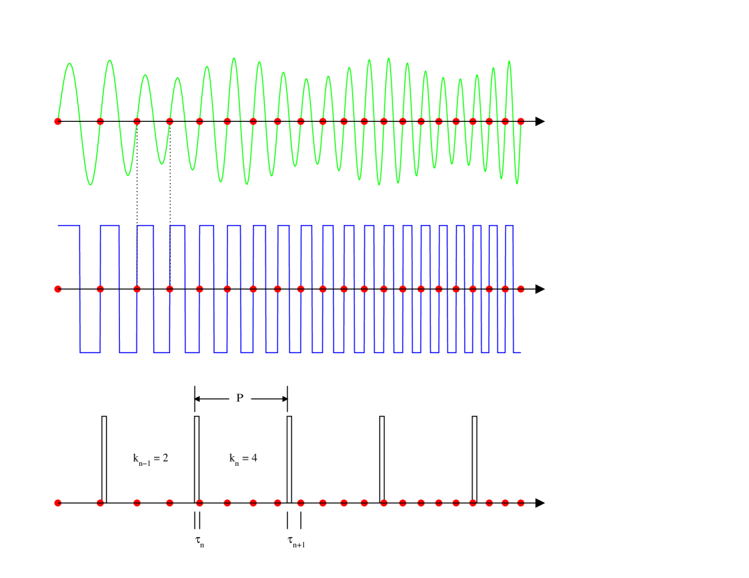
Figure 1: The upper panel shows a typical input to our phase meter: an amplitude varying chirping sinusoid. The conversion of amplitude noise into phase noise can be reduced by amplifying and clamping the initial signal. This is depicted by the chirping square wave in the middle panel. Amplification also makes identification of the positive going zero-crossings (solid disks) simpler. Each of the vertical bars in the bottom panel are tick marks of our fiducial clock, which has a period $P$. The number of zero-crossings $k_{n}$ between each clock tick are recorded by a counter, and the timings $\tau_{n}$ between a clock tick and the first zero-crossing are recorded by our timer. The equations in [2] make use of these definitions.

In general, we need to know the number of signal pulses during the interval between two timing pulses, as well as the time difference at the beginning and end of the timing interval. To obtain this information, we introduce a counting circuit which counts the number of zero-crossings between clock cycles. In this way the number of counts gives the whole number of cycles in the timing interval to within a fraction, and a combination of the time differences gives the correction for the fraction of a cycle. From this collection of counts and times we can reconstruct the phase of the signal at any point in time. Further details on the phase reconstruction algorithm can be found in the literature [1, 2].

Ideally the zero-crossing phasemeter can record the phase as a function of time for any AC signal. Given a certain fixed timing accuracy, the measured phase noise increases linearly with the signal frequency. Therefore if the signal frequency changes by a factor of two, then the measured phase noise likewise will change by a factor of two. This is not an advantageous situation for LISA, where the frequency of the fringe will range from DC to 20 MHz. Therefore it would be wise to fix the signal frequency within some operating bandwidth.

Given the nature of the zero-crossing phasemeter, the determination of the signal phase from the counting of zero-crossings alone would have a larger fractional error for lower frequency signals. However, when one includes the fractional cycle from the timing information it becomes apparent that a lower frequency signal results in a smaller phase error. Nevertheless, we have chosen to make the signal frequency as high as possible to stay away from DC noise sources. The frequency synthesizer which we use to generate our signal has an intrinsic phase noise floor. We have chosen the maximum frequency of our operating band to be the cross-over frequency between the frequency dependent phase noise of our phasemeter and the frequency independent phase noise of our frequency synthesizer.

3 Zero-Crossing Phasemeter Response

We have investigated the response of the zero-crossing phasemeter to various signal types using electronic input signals. In particular we present results for various signal frequencies, frequency sweep rates, and local oscillator bandwidths.

As mentioned in Section 4.1 of [2] the phase noise floor of the zero-crossing phasemeter, determined by the timing resolution of the timer, is linearly proportional to the signal frequency. Therefore it is advantageous to mix the input signal with a local oscillator (LO) to a suitable intermediate frequency (IF) for counting. At low enough frequencies the phase noise level is dominated by intrinsic phase noise in our electronics (as seen in Figure 3 of [2]).

The phase noise that we present is computed by subtracting the known phase of our signal generator from the reconstruction of the phase from our phasemeter (see [2]). From this set of residuals we compute an amplitude spectral density, the phase noise, as a function of frequency from the signal frequency.

3.1 Sweep Rate Investigation

The orbits of the LISA sciencecraft currently under investigation are such that the distances between the sciencecraft change over the course of a year in a roughly sinusoidal manner [3, 4, 5]. The changing distance causes a Doppler shift between the frequencies of the incoming and outgoing laser beams used to produce the LISA fringe signal. Since the distances between the orbits changes over time, the Doppler frequency will vary over the course of a year. The sweep rate is the rate of change of the Doppler frequency.

The exact orbits of the LISA sciencecraft have not been determined. This leaves open the question of how fast the sweep rate might be. However, it is likely that the sweep rate will not exceed a few Hz/s. We have performed a small investigation mapping out the phasemeter response to signals with different sweep rates. Figure 2 contains data of sweeping 1 MHz signals mixed down to about 1 kHz with various sweep rates. When the intermediate frequency (IF) is about to leave the 1—2 kHz band, we instruct the LO to step in frequency by 1 kHz. In this way the IF always remains between 1 and 2 kHz. The spectra shown are for signals with sweep rates of 0.1 Hz/s, 1.0 Hz/s, and 10 Hz/s. For reference, the spectrum from a constant signal frequency is shown. We investigated sweep rates as low as 0.01 Hz/s and as high as 1 kHz/s. For the sweep rates investigated, the phase noise level does not differ from the case of a constant signal frequency.

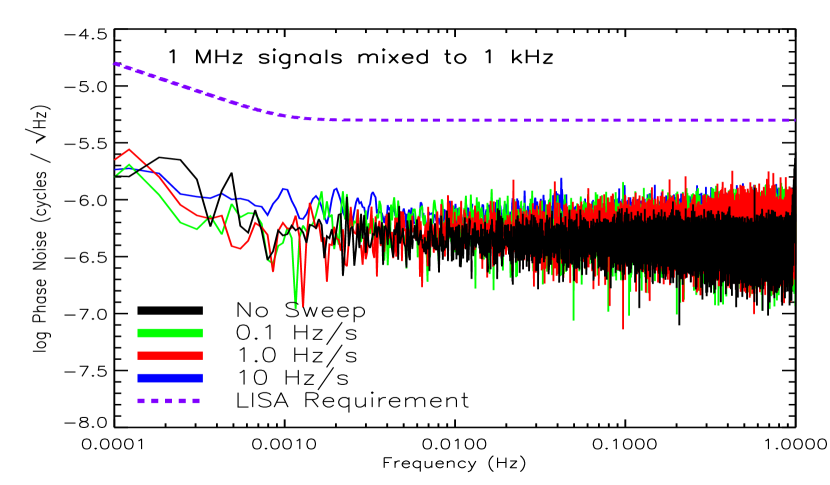
Figure 2: Phase noise spectra for 1 MHz signals with various sweep rates mixed to 1 kHz. We found the phase noise level to be unchanged for sweep rates as fast as 1 kHz/sec.

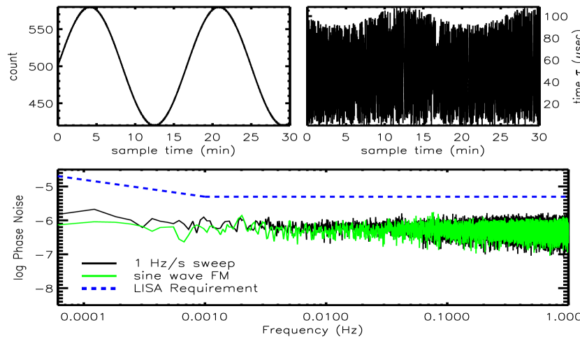
Figure 3: A 1 MHz signal is frequency modulated by a 160 Hz depth 0.001 Hz sinusoid. The signal is mixed down to 1 kHz for phase measurement. The sample frequency is 2 Hz. Top panels: The counts and times follow the frequency modulation of the signal as expected. Bottom panel: Phase noise of the data in the previous panels. The “1 Hz/s sweep” data is for a constantly swept signal at 1 MHz. Having the sweep rate change appears not to affect the phase noise level in this situation.

Of possible concern are jumps in phase of the LO during frequency steps. Our LO has good phase continuity and the jumps in phase are smaller than the resolution of our phasemeter. Feedthrough of these phase jumps to the IF signal are not resolvable.

3.2 Sweep Acceleration Investigation

The distances between the sciencecraft can be approximated as sinusoids in time (see [5] for a preliminary description of the LISA orbits). The period of the sinusoid of the orbits is on the order of one year. For a 1 Hz/s maximum sweep rate, the maximum sweep acceleration will be about 0.1 $\mu$Hz/s². We can simulate a changing sweep rate but only one with a much shorter period. The maximum modulation period of our frequency synthesizer is 1000 seconds. To attain a maximum sweep rate of 1 Hz/s, we frequency modulate our source with a modulation depth of 160 Hz. This yields a sweep acceleration of approximately 6.3 mHz/s². Figure 3 contains the results from this experiment which are as expected: the counts follow a sinusoidal pattern with a mean of 500 (equating to a 1 kHz signal sampled with a 2 Hz clock) and an amplitude of 80 (equating to a modulation depth of 160 Hz). The phase noise appears to be unchanged from that of a signal with a linear frequency ramp at 1 Hz/s.

3.3 Bandwidth Investigation

The phase noise for a sweeping frequency signal is dependent on the operating bandwidth of the phasemeter. In the majority of our data we have implemented a 1 kHz operating bandwidth for our phasemeter. Figure 4 contains phase noise results with various operating bandwidths of our phasemeter between 10 Hz and 1 MHz.

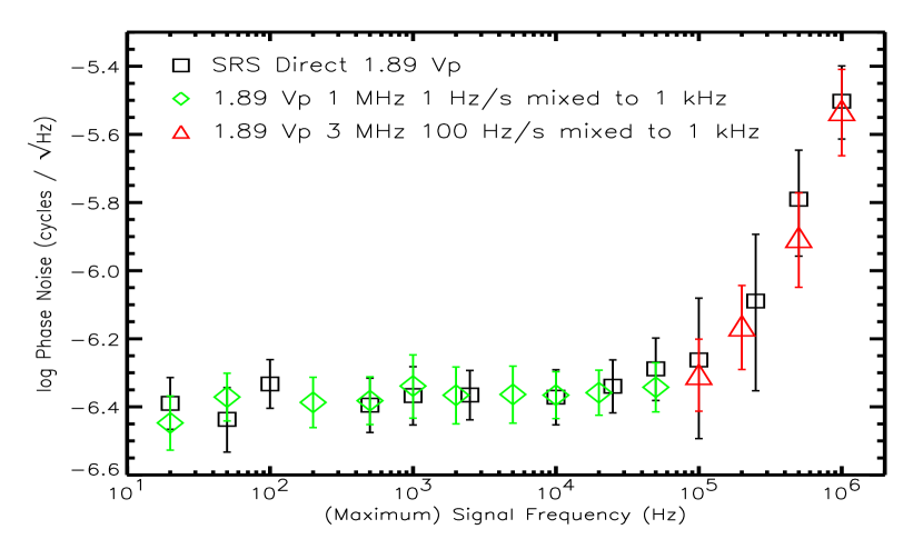
Figure 4: Phase noise data for various operating bandwidths of our phasemeter. The “SRS Direct” data was taken without mixing the signal. The phasemeter operating bandwidth when mixing follows the phasemeter operating bandwidth without mixing.

A 1 MHz signal swept at 1 Hz/s was used to investigate bandwidths smaller than 10 kHz. Above 10 kHz a 3 MHz signal with a sweep rate of 100 Hz/s was used. The LO was instructed to step-up in frequency when the IF reached the limit of the operating band. It is apparent that a smaller bandwidth for the phasemeter is advantageous for keeping the phase noise suppressed. The phase noise floor is the noise of our frequency synthesizer at about $0.42\,\mathrm{{\mu}cycles}/\sqrt{\mbox{Hz}}$ above 1 mHz for a 1.89 volt-peak signal. As shown in the figure, the phase noise appears to follow the phase noise of signals without mixing. The small decrease in phase noise for maximum signal frequencies above about 100 kHz between the triangle and square data is due to the reduced amount of time the signal spent at the higher frequencies. The maximum bandwidth which yields the noise floor of our electronics is approximately 100 kHz. Our choice of a 1 to 2 kHz operating band for our phasemeter seems practical.

4 A LISA Test-Bed Interferometer

The LISA fringe signal has three important qualities: (1) a baseband fringe frequency which ranges from zero to tens of MHz, (2) the fringe sweeps at a rate up to 1 Hz/s, and (3) the fringe has a small signal level resulting from the heterodyning of 100 pW and 1 mW laser beams. Our table-top interferometer has been designed to simulate these three aspects. In addition, our table-top interferometer produces a fringe with a phase noise below $5\,\mathrm{{\mu}cycles}/\sqrt{\mbox{Hz}}$ in the 1 mHz to 1 Hz band, which is the part of the pathlength error budgeted to the phase measurement system [6].

A detailed description of our experimental setup was given in [1]. Figure 5 contains an updated schematic of our interferometer layout. The labeling of components is that of [1]. Included in this schematic are our acoustical stabilization loop described in [1], our frequency generation technique described in [2], our data taking zero-crossing phasemeter with LO feedback, and the new intensity stabilization loop on the bright arm of the interferometer discussed in the following section.

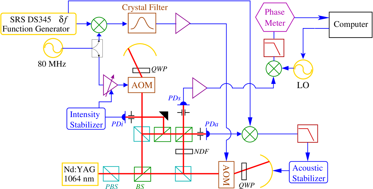
Figure 5: A schematic of our table-top fringe generator with acoustic stabilization, frequency generation, and phasemeter included. The general layout is that of Figure 1 in [1]. The neutral density filter (NDF) reduces the power in the horizontal arm to 100 pW. The intensity stabilization loop is described in the text.

4.1 Constant Frequency Data

One of the first steps in verifying our table-top interferometer is to demonstrate the LISA phase measurement requirement of a constant frequency signal created by heterodyning a low power laser beam with a high power laser beam. We adjust the power differential between the arms by using neutral density filters. Although our commercial laser has a built-in intensity noise eater, residual laser intensity noise, at frequencies below 1 MHz, in the bright arm of the interferometer dominates the phase noise level for large power differentials (see Figure 6 below). The relationship between the phase noise and the power differential is easy to derive.

The total electric field at the photoreceiver is the sum of the contributions from each arm of the interferometer. If we write the electric field in each arm of the interferometer as $E(x,t)=\sqrt{P}\,e^{\mathring{\imath}(kx-2\pi ft+\phi)}$ then the intensity measured at the photoreceiver will be

$$P_{\mathrm{meas}}=P_{1}+P_{2}+2\,\sqrt{P_{1}P_{2}}\,\cos\,(2\pi\,\delta\!f\,t-\delta\phi)\,,$$ (1)

where $\delta\!f=f_{2}-f_{1}$ and $\delta\phi=\phi_{2}-\phi_{1}$. The fringe signal is represented in the above equation by the sinusoidal cross term. The other two terms are DC offsets. The frequency of the fringe is naturally the difference frequency between the two arms of the interferometer set by our frequency synthesizer. The phase difference $\delta\phi$ can be adjusted by dithering the spherical mirror at the end of one arm of the interferometer.

We write the power in the dim arm as $P_{2}=\rho\,P$, where $\rho$ is the power ratio, or inverse power differential, and the power in the bright arm is $P_{1}=P$. With this definition the amplitude of the fringe becomes $P\sqrt{\rho}$, assuming a 50-50 beamsplitter. Therefore the amplitude of the fringe is inversely proportional to the square root of the power differential between the arms of the interferometer. Since the phase noise level, $\phi_{n}$, is proportional to the fractional error, we obtain

$$\phi_{n}\,(\mathrm{cycles}/\sqrt{\mbox{Hz}})\propto\frac{V_{n}}{P\sqrt{\rho}}\,,$$ (2)

where $V_{n}$ is the intrinsic noise level of our electronics. We see in this relation that the phase noise level is proportional to the square root of the power differential which is consistent with the data shown in Figure 6.

Since the dim beam is reduced in power by several orders of magnitude, the main contributor of amplitude noise in the final fringe signal is the intensity noise of the bright beam. Before the recombining beamsplitter the bright beam passes through a “pick-off” beamsplitter. This beamsplitter is actually a 50-50 beamsplitter so that half of the light in the bright beam is incident upon a separate photoreceiver, PDi (see Figure 5), which is used for the stabilization of the intensity of the laser in the bright beam.

The output of PDi goes to a servo controller which attempts to remove variations in the intensity of the received light. Intensity control is accomplished by changing the amplitude of the frequency input to the AOM in the bright arm. This gain control is symbolized in the schematic of Figure 5 as an amplifier with an arrow through it.

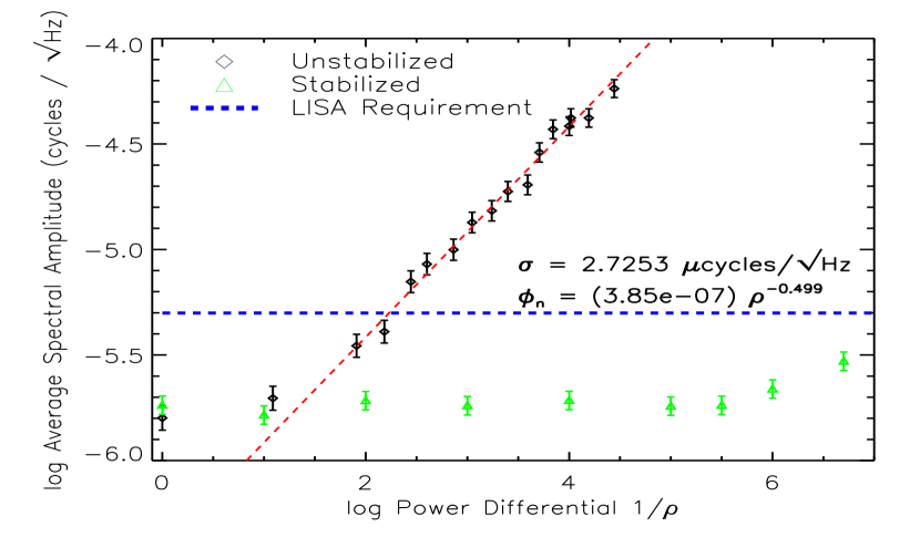
Figure 6: Integrated phase noise in the 1–100 mHz band for a range of power differentials between the arms of the interferometer. Without intensity stabilization the phase noise rises as the square root of the power differential as expected.

Figure 6 contains phase noise levels of 50 kHz fringe signals taken with various power differentials. With the intensity stabilization servo off the data follows the relation in Equation (2). With the intensity stabilization servo active the intensity noise of the laser is no longer the dominant noise source for power differentials greater than 10. The intensity noise resumes the role of being the largest noise source for power differentials greater than about one million.

With the intensity stabilization servo active the power level in the bright arm of the interferometer drops to 0.5 mW in order to facilitate the suppression of intensity noise. The power in the dim arm is unchanged from the target power level of 100 pW. These power levels create a power differential of five million. The required power differential has been stated historically to be ten million. This comes from the ratio of 1 mW and 100 pW. There is no hard and fast requirement on there being 1 mW of light used from the local laser beam. Therefore we feel confident that 0.5 mW is sufficient for our demonstration.

4.2 Timing a LISA-like Fringe

We are now in position to produce a full LISA-like fringe from our table-top interferometer. We choose a collection of baseband frequencies ranging from 50 kHz to 20 MHz for data collection. For each baseband frequency the signal frequency slowly sweeps at a rate of 1 Hz/s. In addition, there is a power differential between the arms of the interferometer of five million. Phase noise spectra of the resulting data are shown in Figure 7. For this data we have instructed the LO to keep the IF between 1 and 2 kHz.

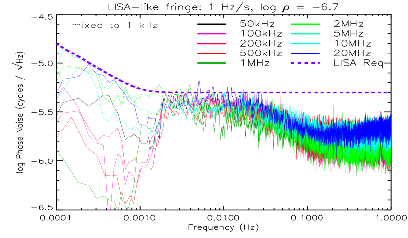
Figure 7: Phase noise spectra of LISA-like fringes at a range of baseband frequencies. The LO was instructed to keep the IF between 1 and 2 kHz. The power levels of the arms of the interferometer are 0.5 mW and 100 pW, resulting in a power differential of five million. The fringe sweep rate is 1 Hz/s.

All of the spectra shown in Figure 7 have the same general phase noise profiles at frequencies above 2 mHz from the fringe frequency. With the intensity stabilization servo active the phase noise is dominated by electronic noise from the frequency generation technique. We are meeting the LISA requirement of 5 $\mathrm{{\mu}cycles}/\sqrt{\mbox{Hz}}$ between 1 mHz and 1 Hz for all baseband frequencies examined. Also, the noise only rises as roughly $f^{-1/2}$ below 1 mHz, which is well below the assumed increase of $f^{-2}$ that would be allowed for LISA.

It is interesting to note that in general there appears to be less phase noise at frequencies below 2 mHz from the fringe frequency for low frequency fringes. We are unsure of the cause of this, and have not been able to reproduce these low-frequency stable phase signals. Our subsequently taken data always rises as $f^{-1/2}$ at low frequencies. Note that the data presented are each the average of four 4.5-hour long data sets. At 0.1 mHz there are 1.6 cycles in 4.5 hours, and consequently there are 6.6 cycles in each spectra of Figure 7. In contrast for a 1 mHz signal there are 66 cycles in each spectra. The smaller number of cycles might lead one to expect that the error at 0.1 mHz would be 3 times larger than the error at 1 mHz. In actuality, the variance of each power spectrum, at all frequencies, is roughly the mean power level. For our spectra the mean power level is about 2 $\mathrm{{\mu}cycles}/\sqrt{\mbox{Hz}}$ integrated over the $10^{-4}$ to 1 Hz band. This error should be kept in mind when considering the suspiciously low phase noise values below 2 mHz.

4.3 Sweeping the Local Oscillator

In Section 3.3 we examined cases where we allowed the IF to roam over the full practical range of the phasemeter operating band as well as confining the IF to a small bandwidth. We can take that investigation one step further and have the LO continuously sweep in frequency. Phase delays through the crystal filter used in our frequency generation technique (described in Section 3.2 of [2]) very slightly alter the actual sweep rate of the fringe signal. Since the sweep rate is not exactly equal to the sweep rate programmed into our frequency synthesizer, we feedback to the LO during data taking, changing the sweep rate until it matches the sweep rate of the fringe signal. In this way the IF remains constant in frequency. There is a similar situation in LISA where the sweep rates of the fringe signals may not be known exactly. If LO tracking is to be used, then a similar feedback loop to ours will need to be employed. We found that the final phase noise was unchanged from the case of a constant fringe frequency.

5 Items of Concern

There are several aspects of our experimental simulation which are different from LISA. In this section we discuss the following items of concern: (1) correlation between the photoreceivers PDs and PDa at the combining beamsplitter, (2) laser frequency noise, (3) aliasing of noise due to our analog demodulation and decimation of sampling, and (4) effects of tones on the LISA fringe.

5.1 Correlation of Output Beams

Observation of Figure 5 indicates that the signal observed on PDs should be quite similar to $\delta\!f$ due to the acoustical stabilization feedback loop. If the two signals were identical, then the inclusion of a table-top interferometer in our experiment serves no practical purpose. However, this is not the case. We have measured the correlation between PDa and PDs to be 80% at 1 mHz, falling rapidly to 0% by 7 Hz away from $\delta\!f$.

The correlation between PDs and PDa not withstanding, our interferometer does provide some aspects of realism. In practice we are looking for noise sources which are not common-mode between PDs and PDa. Naturally these noise sources, and the methods we have developed to deal with them, may be of importance for LISA. In particular, the shot noise and electronic noise in each of our photoreceivers is not common-mode and will appear in our measurement.

In addition, we use a realistic laser (although we ignore laser frequency noise, see below), with a power differential between the arms of the interferometer, and a fringe beatnote ranging in frequency from nearly DC to 20 MHz, sweeping at a rate of 1 Hz/s. Residual laser amplitude noise is present in our experimental setup and is a dominant noise source for large power differentials between the arms of the interferometer. A technique for suppressing amplitude noise will be necessary on LISA, although a technique similar to ours will most likely not be used. However, it is probable that for ground testing of the LISA sciencecraft a technique similar to ours may be utilized.

5.2 Laser Frequency Noise

Laser frequency noise is essentially absent from our experiment since we use only one laser. However, we can simulate the effect of laser frequency noise by injecting noise into our interferometer by using a noisy $\delta\!f$ from our SRS DS345 frequency synthesizer. Any noise on this signal appears on our photoreceiver and will not be removed by our acoustic stabilization loop. We have done this experiment, and the final phase noise level matches that expected due to the noisy source. Of course our assumption in our result is that laser frequency noise adds linearly and therefore can be removed by this technique to the required precision from time-delay interferometry (TDI, see e.g., [7, 8] and references therein).

5.3 Aliasing of Noise

There are two separate issues regarding aliasing. In particular, the aliasing of laser frequency noise is of concern. The first issue is due to decimation of sampling. If we sampled at the same frequency as the IF then we would obtain all the phase information possible. However, since we sample the phase at our clock frequency, which is considerably less than the IF, one might expect that we are losing phase information. However, we count the zero-crossings between timing measurements and therefore do not actually lose any phase information. In effect we average the phase over the number of cycles between clock ticks.

The issue of aliasing regarding decimation is that signals of frequencies higher than our clock frequency will be aliased into our measurement band. Indeed, we see this effect in simple experiments, such as the following: a 1 kHz sinusoid is phase modulated with a $10^{\circ}$ 11 Hz signal. Our clock frequency is set to 10 Hz. The resulting phase noise spectrum shows a peak at 1 Hz, which is the 11 Hz signal aliased by 10 Hz. However, uncorrelated signals which alias into our measurement band will be suppressed. This is because we are effectively averaging between clock ticks as mentioned above. In this manner the noise at frequencies above our clock frequency aliased into our measurement band do not adversely effect the measured phase noise level.

The second aliasing issue is due to the analog demodulation performed to bring the frequency $\delta\!f$ to a suitable IF for our phasemeter. Laser frequency noise at frequencies much larger than our IF away from the carrier prior to demixing will appear at negative frequencies afterward. Since our phasemeter only detects positive frequencies, this DC-wrapped noise will adversely affect the measured phase.

The issue of DC-wrapping aliasing is not a deterrent for the zero-crossing phasemeter. Time-delay interferometry (TDI, see e.g., [7, 8] and references therein) is the process by which laser frequency noise will be corrected for in LISA. In TDI two phasemeter outputs are combined with a time offset in order to subtract the laser frequency noise contribution to the phase measurement.

Naive thinking might lead one to believe that aliased laser frequency noise would spell the end for TDI. However, even though noise is being aliased into the measurement band, it is being aliased in the same way in each measurement. Therefore the construction of TDI variables will still correct laser frequency noise, even though that noise has been aliased.

We have performed TDI-like experiments with our table-top interferometer and zero-crossing phasemeter. In the most complex of these experiments we inject a noisy signal into our interferometer. This signal is mixed down to a suitable IF for our phasemeter. In this process we would expect that aliased noise from the analog demodulation of the high frequency fringe signal will dominate the phase noise measurement. Indeed it does. We take two such data sets. The noise is programmed, therefore it is identical in the second data set. However, due to slight timing errors in the computer GPIB communication process the noise will be time-delayed. In software we fit for the time-delay between the two data sets. After subtraction the noise level is $\sqrt{2}$ higher than the un-noisy signal from the interferometer as expected.

It should be mentioned that we have relied on the response of our phasemeter to be nearly identical during the two data sets. The precision of our phasemeter is crucial in allowing us to subtract the time-delayed noisy signals to below the shot noise level of our interferometer. A slightly more advanced test of this TDI-like experiment would be with two separate phasemeters measuring simultaneously. This would be possible in our current setup if we added a phasemeter at the PDa port of our interferometer.

We have determined that aliased laser frequency noise can be successfully canceled. Therefore the most serious aliasing issues discussed above are not deterrents from using the zero-crossing phasemeter in LISA. However, shot noise or technical noise that is DC-wrapped aliased in would not be corrected for in the TDI process, and therefore the noise level will be $\sqrt{2}$ higher than the shot noise alone, just as in our demonstration.

5.4 Communication Tones

Our table-top interferometer can be easily modified to include USO sidebands, ranging tones, and digital data modulations on the laser beam. We have performed the necessary modifications and will be presenting our results in a another article [9].

6 Summary

We have constructed a table-top interferometer which produces LISA-like fringes. These fringes have the following properties: (1) a baseband fringe frequency which ranges from 50 kHz to 15 MHz, (2) the fringe frequency sweeps at a rate of 1 Hz/s, and (3) a small signal level resulting from the heterodyning of a 100 pW laser beam and a 0.5 mW laser beam.

We have verified the power differential-phase noise relation Equation (2) and have reduced this dependence by the addition of an intensity stabilization servo for the bright arm of the interferometer (Figures 5 and 6).

We have demonstrated that the fringes produced by our fringe generator have a displacement noise less than the LISA allocation to phase measurement, namely 5 pm/$\sqrt{\mbox{Hz}}$ from 1 mHz to 1 Hz, rising slower than $f^{-1/2}$ at lower frequencies (Figure 7).

We have investigated the effects of tracking the slowly varying fringe with the local oscillator to produce a constant frequency signal for our phasemeter. As will be the case for LISA we found that small corrections to the LO sweep rate were needed to properly account for the changing fringe rate. Upon implementing these modifications we were able to attain a constant frequency IF which had a phase noise level identical to the case of a non-sweeping fringe signal.

References

References

- [1] O Jennrich, R T Stebbins, P L Bender, and S Pollack, “Demonstration of the LISA phase measurement principle”, Class. Quantum Grav.18 (2001), 4159–4164.
- [2] S E Pollack, O Jennrich, R T Stebbins, and P Bender, “Status of LISA Phase Measurement work in the U.S.”, Class. Quantum Grav.20 (2003), S291–S200.
- [3] S M Merkowitz, A Ahmad, T T Hyde, T Sweetser, J Ziemer, S Conkey, W Kelly III, and B Shirgur “LISA Propulsion Module Separation Study”, Class. Quantum Grav.22 (2005), S413–S419.
- [4] T H Sweetser, “And end-to-end trajectory description of the LISA mission”, Class. Quantum Grav.22 (2005), S429–S435.
- [5] S P Hughes, “Preliminary Optimal Orbit Design for the Laser Interferometer Space Antenna (LISA)”, Proceedings of the 25th Annual AAS Guidance and Control Conference (Breckenridge, CO) (R D Culp and S D Jolly, eds.), Advances in the Astronautical Sciences, vol. 111, February 2002, pp. 61–78.
- [6] P L Bender, K V Danzmann, and the LISA Study Team, “Laser Interferometer Space Antenna for the Detection of Gravitational Waves, Pre-Phase A Report”, MPQ-233 2nd ed., Max-Planck Institute for Quantum Optics, Garching, Germany, 1998.
- [7] M Tinto, F B Estabrook and J W Armstrong, “Time delay interferometry with moving spacecraft arrays”, Phys. Rev. D 69 (2004), 082001.
- [8] M Tinto, D A Shaddock, J Sylvestre and J W Armstrong, “Implementation of time-delay interferometry for LISA”, Phys. Rev. D 67 (2003), 122003.
- [9] S E Pollack and R T Stebbins, “A Demonstration of LISA Laser Communication”, submitted to Class. Quantum Grav..