The photon vacuum polarization effect in curved spacetime leads to birefringence, i.e. the photon velocity becomes $c\pm\delta c$ depending on its polarization. This velocity shift then results in modified photon trajectories. We find that photon trajectories are shifted by equal and opposite amounts for the two photon polarizations, as expected by the sum rule [5]. Therefore, the critical circular orbit at $u=1/3M$ in Schwarzschild spacetime, is split depending on polarization as $u=1/3M\pm A\delta(M)$ (to first order in $A$), where $A$ is a constant found to be $\sim 10^{-32}$ for a solar mass blackhole. Then using general quantum modified trajectory equations we find that photons projected into the blackhole for a critical impact parameter tend to the critical orbit associated with that polarization. We then use an impact parameter that is lower than the critical one. In this case the photons tend to the event horizon in coordinate time, and according to the affine parameter the photons fall into the singularity. This means even with the quantum corrections the event horizon behaves in the classic way, as expected from the horizon theorem [5]. We also construct a quantum modified Schwarzschild metric, which encompasses the quantum polarization corrections. This is then used to derive the photons general quantum modified equations of motion, as before. When this modified metric is used with wave vectors for radially projected photons we obtain the classic equations of motion, as expected, as radial velocities are not modified by the quantum polarization correction.

Chapter 1 Introduction

1.1 General Relativity

Since the birth of special relativity, in 1905, the nature of space and time has been demoted to a relative entity, known as spacetime, which is stretched and contracted depending on an observer’s frame of reference, while the speed of light, $c$, has taken the pedestal of an absolute and universal speed limit, unaffected by any transformation of reference frame. From this emerged a generalized theory of relativity, which portrayed the gravitational field in a new and revolutionary way: where it didn’t depend on a propagating field but on the nature of spacetime itself. In this view matter (or energy) is said to curve and modify the surrounding spacetime, this then results in photons and particles tracing out shortest paths between two points, known as geodesics. Therefore, gravitational forces become a manifestation of the curved spacetime due to the presence of matter [4, 3]. In this general relativistic framework spacetime is described by the metric $g_{\mu\nu}$ and the motion of particles are described by the interval equation:

$$k^{2}=g_{\mu\nu}k^{\mu}k^{\nu}\qquad\Rightarrow\qquad\begin{array}[]{c}>0\qquad\textmd{Time-like ($c<1$)}\\ =0\qquad\textmd{Light-like ($c=0$)}\\ <0\qquad\textmd{Space-like ($c>1$)}\\ \end{array}$$ (1.1)

where $k^{\mu}=\frac{dx^{\mu}}{d\tau}$. For flat spacetime or a local inertial frame (LIF), where $g_{\mu\nu}$ is replaced by the diagonal Minkowski metric $\eta_{\mu\nu}=(1,-1,-1,-1)$, the interval equation becomes:

$$k^{2}=\eta_{\mu\nu}k^{\mu}k^{\nu}=\frac{dt}{d\tau}^{2}-\frac{dx}{d\tau}^{2}-\frac{dy}{d\tau}^{2}-\frac{dz}{d\tau}^{2}$$ (1.2)

for $c=1$. Apart from resolving the problems associated with Newtonian mechanics, such as describing the perihelion advance of Mercury, the strongest aspect of general relativity was its predictive power. One of its most radical claims, and the building blocks of the theory itself, was that gravitational fields affect radiation, which was then confirmed through the observation of starlight deflection by the sun. From this emerged some profound and fantastic possibilities such as black holes and gravitational lensing. The gravitational effect on light rays also leads to the possibility that photons could follow stable orbits around stars (discussed in chapter 2), and it’s this possibility in which we will be interested.

1.2 QED in a Curved Spacetime

Even though photon trajectories are modified in a curved spacetime, and the resulting curved paths are described by general relativity, this bending of light was, for a long time, considered to have no effect on the velocity of the photon. This view shifted slightly when, in 1980, Drummond and Hathrell[1] proposed that a photon propagating in a curved spacetime may, depending on its direction and polarization, travel with a velocity that exceeds the normal speed of light $c$. This change in velocity would then result in trajectories other then the ones described by "classical" general relativity. This effect is simply described as a modification of the light cone in a LIF:

$$k^{2}=\eta_{\mu\nu}k^{\mu}k^{\nu}=0\quad\rightarrow\quad(\eta_{\mu\nu}+\alpha\sigma_{\mu\nu}(R))k^{\mu}k^{\nu}$$ (1.3)

Where $\alpha$ is the fine structure constant and $\sigma_{\mu\nu}(R)$ is a modification to the metric that depends on the Riemann curvature at the origin of the LIF. This correction is seen to arise from photon vacuum polarizations in a curved space time, Fig. 1.1.

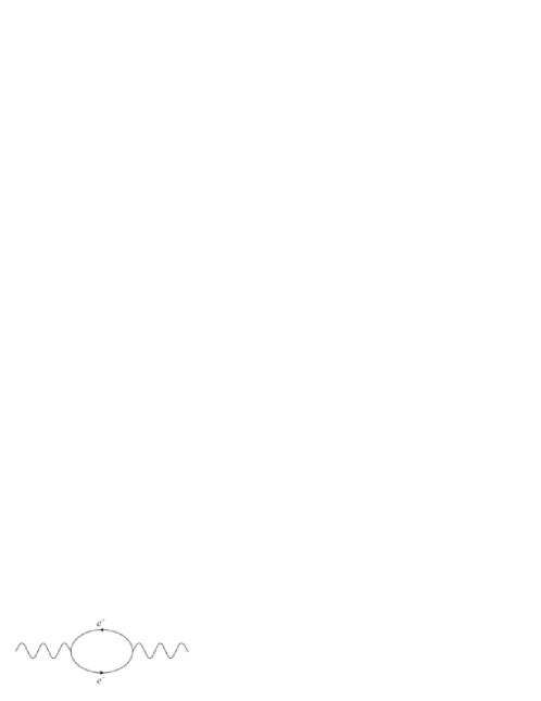
Figure 1.1: First order, $\alpha$, vacuum polarization Feynman diagram contributing to the photon propagator

Qualitatively it can be thought of as a photon splitting into a virtual $e^{+}e^{-}$ pair, so at the quantum level it is characterized by the Compton wavelength $\lambda_{c}$; then, when this quantum cloud of size $\mathcal{O}(\lambda_{c})$ passes through a curved spacetime its motion would be affected differently to that described by general relativity, possibly in a polarization-dependent way [5].

This effect of vacuum polarization is considered through the effective action:

$$S=S_{1}+S_{2}$$ (1.4)

where $S_{1}$ is the Maxwell electromagnetic action in curved space time:

$$S_{1} = -\frac{1}{4}\int d^{4}x\sqrt{-g}F_{\mu\nu}F^{\mu\nu}$$

$$F_{\mu\nu} = \partial_{\mu}A_{\nu}-\partial_{\nu}A_{\mu}$$ (1.5)

and $S_{2}$ is the part of the action that incorporates the effects of virtual electron loops in a background gravitational field. As we are only concerned with the propagation of individual photons it must be quadratic in $A_{\mu}$, and the constraint of gauge invariance then implies that it must depend on $F_{\mu\nu}$ rather than $A_{\mu}$. Also, as the virtual loops give the photon a size of $\lambda_{c}$, $S_{2}$ can be expanded in powers of $\lambda_{c}^{2}=m^{-2}$, thus the lowest term in the expansion would be of order $m^{-2}$, which is the term corresponding to one electron loop. With these constraints there are only four independent gauge invariant terms, which can be chosen to be:

$$S_{2} = \frac{1}{m^{2}}\int d^{4}x\sqrt{-g}(aRF_{\mu\nu}F^{\mu\nu}+bR_{\mu\nu}F^{\mu\sigma}F^{\nu}_{\sigma}$$ (1.6)

$$+ cR_{\mu\nu\sigma\tau}F^{\mu\nu}F^{\sigma\tau}+dD_{\mu}F^{\mu\nu}D_{\sigma}F^{\sigma}_{\nu})$$

The first three terms represent a direct coupling of the electromagnetic field to the curvature, and they vanish in flat-spacetime. The fourth, however, is also applicable in the case of flat-spacetime, and represents off-mass-shell effects in the vacuum polarization. In [1] the values for $a$, $b$, $c$, and $d$ have been determined to $\mathcal{O}(e^{2})$. The constant $d$ is obtained by comparing the coefficient of the renormalized flat-spacetime photon propagator associated with the Feynman diagram in Fig. 1.1 to the result of the same order given by the effective action $S$; and $a$, $b$, and $c$ are obtained by comparing the coefficients of the coupling of a graviton to two photons to the same result obtained from $S_{2}$. In this way the constants are given as:

$$a=-\frac{5}{720}\frac{\alpha}{\pi}\qquad b=\frac{26}{720}\frac{\alpha}{\pi}\qquad c=-\frac{2}{720}\frac{\alpha}{\pi}\qquad d=-\frac{24}{720}\frac{\alpha}{\pi}$$ (1.7)

Then, as the equations of motion for the electromagnetic field are given by:

$$\frac{\delta S}{\delta A_{\mu}(x)}=0$$ (1.8)

using the modified action (1.4) we find:

$$D_{\mu}F^{\mu\nu}+\frac{\delta S_{2}}{\delta A_{\mu}}=0$$ (1.9)

From this we can see that $D_{\mu}F^{\mu\nu}$ is of $\mathcal{O}(e^{2})$, therefore, the term with coefficient $d$ in Eqn. (1.6) will be of $\mathcal{O}(e^{4})$, hence we can omit it from the final equation of motion. In this way we find [7]:

$$D_{\mu}F^{\mu\nu}-\frac{1}{m_{e}^{2}}[2bR_{\mu\lambda}D^{\mu}F^{\lambda\nu}+4cg^{\nu\tau}R_{\mu\tau\lambda\rho}D^{\mu}F^{\lambda\rho}]=0$$ (1.10)

which is the Maxwell equation in curved spacetime, incorporating the coupling of curvature with vacuum polarization effects. Using this modified Maxwell equation and the methods of geometric optics (described in Chapter 3) it is possible to derive the quantum modified light cone and geodesic equations. Then, using these, we are able to determine the quantum modified trajectories in curved spacetime.

1.3 The Equivalence Principle and Causality

The equivalence principle exists in two forms: weak and strong. The weak equivalence principle states that at each point in spacetime there exists a local Minkowski frame, which is a fundamental requirement of general relativity. The strong equivalence principle (SEP), on the other hand, states that the laws of physics are the same in all LIFs at different points in spacetime, and at the origin of each LIF they take the special relativistic form. Then the coupling of curvature to the electromagnetic field in the effective action, Eqn. (1.4), is a violation of the SEP. Due too this violation of the SEP, QED in curved spacetime remains a causal theory - despite the modification to the physical light cone.

This can be seen more clearly by considering Global Lorentz invariance (GLI), which is the special relativistic equivalent of the SEP. In special relativity GLI states that faster than light signals automatically imply the possibility of unacceptable closed-time-loops, Fig. 1.2. That is, if you can send a signal backwards in time in one frame, then it should be possible in any frame. However, if you break this GLI, a signal backwards in time in one frame does not automatically imply you can send a signal backwards in time from any frame. Therefore, in the case of QED in curved spacetime, due to the breakdown of the SEP we retain the fundamental property of causality: faster than light signals can be seen to go backwards in time in a certain frame, but this no longer implies that you can send a signal backwards in time from any frame. Thus, in this case, spacelike motion does not necessarily imply a causality violation.

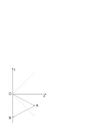
Figure 1.2: An unacceptable closed-time-loop.

1.4 Critical Stable Orbits

One of the simplest curved spacetimes is the (Ricci-flat) Schwarzschild spacetime, which describes the spherically symmetric geometry outside a star. The geometry of such a spacetime structure is given by the line interval:

$$ds^{2}=(1-\frac{2M}{r})dt^{2}-(1-\frac{2M}{r})^{-1}dr^{2}-r^{2}d\theta^{2}-(r^{2}\sin^{2}\theta)d\phi^{2}$$ (1.11)

In this spacetime the equations of motion, derived for $k^{2}=0$, have a special solution for null geodesics. This solution describes a light ray in a circular orbit with a radius $r=3M$ and an associated critical impact parameter. Therefore, a photon projected from $r\rightarrow\infty$ with the critical parameter tends to the stable circular orbit by spiralling around it. But, in the context of vacuum polarization effects, we may derive the null equation of motion using the quantum modified Maxwell equation. In this way the orbit equation should give us stable circular orbits that are dependent on the photon polarization, i.e. splitting the circular orbit depending on polarization. Therefore, a photon coming in from $r\rightarrow\infty$, with a particular polarization and impact parameter, should tend to its associated critical stable orbit by spiralling around it in the classic way.

Chapter 2 Null Dynamics in Schwarzschild Spacetime

In this chapter we will give a brief overview of null dynamics in Schwarzschild spacetime. Starting with the geodesic equations and the line interval for photons we will derive the orbit equation, which will then be used to determine the critical stable orbit for photons and the associated impact parameter. We will then go on to show that decreasing the impact parameter, from the critical value, causes the photon trajectory, given as a function of $\phi$, to spiral into the singularity, but as a function of $t$ it tends to the event horizon. The main aim of this chapter is to familiarise ourselves with the classical solutions of photon trajectories in Schwarzschild spacetime, so we can then compare the equivalent results for the quantum modified case.

2.1 Equations of Motion

When we consider motion in a plane, where $\theta=\frac{\pi}{2}$ and $\dot{\theta}=\ddot{\theta}=0$, the geodesic equations for Schwarzschild spacetime, (A.10)-(A.13), can written as:

$$(1-\frac{2M}{r})\ddot{t}+\frac{2M}{r^{2}}\dot{r}\dot{t}=0$$ (2.1)

$$\frac{M}{r^{2}}\dot{t}^{2}-r\dot{\phi}^{2}+(1-\frac{2M}{r})^{-1}\ddot{r}-\frac{M}{r^{2}}(1-\frac{2M}{r})^{-2}\dot{r}^{2}=0$$ (2.2)

$$2r\dot{r}\dot{\phi}+r^{2}\ddot{\phi}=0$$ (2.3)

And the spacetime line interval becomes:

$$(1-\frac{2M}{r})\dot{t}^{2}-(1-\frac{2M}{r})^{-1}\dot{r}^{2}-r^{2}\dot{\phi}^{2}=K$$ (2.4)

where $K=0$ for photons and $\pm 1$ for space-like or time-like motion. Now, to derive the orbit equation $\frac{du}{d\phi}$ we use Eqns. (2.1), (2.3) and the interval equation (2.4), in the simplified form:

$$0 = \ddot{t}+\frac{2M}{r^{2}}(1-\frac{2M}{r})^{-1}\dot{r}\dot{t}$$ (2.5)

$$0 = \ddot{\phi}+\frac{2\dot{r}}{r}\dot{\phi}$$ (2.6)

$$K(1-\frac{2M}{r}) = -\dot{r}^{2}+(1-\frac{2M}{r})^{2}\dot{t}^{2}-r^{2}(1-\frac{2M}{r})\dot{\phi}^{2}$$ (2.7)

In order to specify photon trajectories we can set $K=0$ at anytime, however, then $\tau$ would be interpreted as an affine parameter and not proper time. To proceed we divide (2.5) by $\frac{dt}{d\tau}$ and (2.6) by $\frac{d\phi}{d\tau}$:

$$0 = \frac{\ddot{t}}{\dot{t}}+\frac{2M}{r^{2}}(1-\frac{2M}{r})^{-1}\dot{r}$$ (2.8)

$$0 = \frac{\ddot{\phi}}{\dot{\phi}}+\frac{2\dot{r}}{r}$$ (2.9)

These can written as:

$$0 = \frac{d}{d\tau}(\ln{\dot{t}}+\ln(1-\frac{2M}{r}))$$ (2.10)

$$0 = \frac{d}{d\tau}(\ln{\dot{\phi}}+\frac{2\dot{r}}{r})$$ (2.11)

Then, solving these we have:

$$\dot{t} = (1-\frac{2M}{r})^{-1}E$$ (2.12)

$$\dot{\phi} = \frac{J}{r^{2}}$$ (2.13)

Where $E$ and $J$ are constants of integration denoting total energy and angular momentum about an axis normal to the plane $\theta=\pi/2$. Now, using Eqns. (2.12) and (2.13) to substitute for $\dot{t}$ and $\dot{\phi}$ in Eqn (2.7) and rearranging, we have:

$$\dot{r}^{2}+r^{2}(1-\frac{2M}{r})\frac{J^{2}}{r^{4}}+K(1-\frac{2M}{r})=(1-\frac{2M}{r})^{2}(1-\frac{2M}{r})^{-1}E^{2}$$ (2.14)

Rearranging and simplifying, this becomes:

$$(\frac{dr}{d\tau})^{2}+(1-\frac{2M}{r})(K+\frac{J^{2}}{r^{2}})=E^{2}$$ (2.15)

$$(\frac{dr}{d\tau})=E[1-(1-\frac{2M}{r})(\frac{K}{E^{2}}+\frac{J^{2}}{E^{2}r^{2}})]^{\frac{1}{2}}$$ (2.16)

We now have the components of the four momentum $P^{\alpha}$ in spherical polar coordinates

$$P^{\alpha} = (\dot{t},\dot{r},\dot{\theta},\dot{\phi})$$ (2.17)

$$= E(F^{-1},[1-F(\frac{K}{E^{2}}+\frac{D^{2}}{r^{2}})]^{\frac{1}{2}},0,\frac{D}{r^{2}})$$

where $D=\frac{J}{E}$ is the impact parameter, $F=(1-\frac{2M}{r})$ and $K=0$ for photons and $K=+1$ for particles.

2.1.1 Orbit Equation

In order to derive orbit equations that are physically understandable we need to represent them as $r(\phi)$, $r(t)$ and $\phi(t)$. In this form we can analyse the orbit paths as a function of rotational angle $\phi$ and the time taken to reach a certain point along the angle. Therefore, by using

$$\frac{dr}{d\tau}=\frac{dr}{d\phi}\cdot\frac{d\phi}{d\tau}=\frac{dr}{d\phi}\frac{J}{r^{2}}$$ (2.18)

we can rewrite (2.15) as

$$E^{2} = (\frac{dr}{d\phi})^{2}\frac{J^{2}}{r^{4}}+(1-\frac{2M}{r})(K+\frac{J^{2}}{r^{2}})$$

$$\Rightarrow\qquad(\frac{dr}{d\phi})^{2} = (E^{2}-K)\frac{r^{4}}{J^{2}}+2MK\frac{r^{3}}{J^{2}}-r^{2}+2Mr$$ (2.19)

Now, transforming $u=r^{-1}$, so at $r=\infty$ we have $u=0$, Eqn. (2.19) becomes:

$$(\frac{du}{d\phi})^{2}r^{4} = (E^{2}-K)\frac{r^{4}}{J^{2}}+2MK\frac{r^{3}}{J^{2}}-r^{2}+2Mr$$

$$(\frac{du}{d\phi})^{2} = \frac{(E^{2}-K)}{J^{2}}+2MK\frac{u}{J^{2}}-u^{2}+2Mu^{3}$$ (2.20)

Doing similar manipulation for $\phi(t)$ we have

$$\frac{d\phi}{dt}=\frac{d\phi}{d\tau}\cdot\frac{d\tau}{dt}$$ (2.21)

and using Eqns. (2.12) and (2.13) in this, and transforming $u=\frac{1}{r}$, we have:

$$\frac{d\phi}{dt}=\frac{D}{r^{2}}(1-\frac{2M}{r})=Du^{2}(1-2Mu)$$ (2.22)

Finally, we can determine $u(t)$ by inserting:

$$\frac{du}{d\phi}=\frac{du}{dt}\cdot\frac{dt}{d\phi}=\frac{du}{dt}[Du^{2}(1-2Mu)]^{-1}$$ (2.23)

into Eqn. (2.20), which gives

$$(\frac{du}{dt})^{2}=[Du^{2}(1-2Mu)]^{2}[\frac{(E^{2}-K)}{J^{2}}+2MK\frac{u}{J^{2}}-u^{2}+2Mu^{3}]$$ (2.24)

Now, the Eqns. (2.20), (2.22) and (2.24) are the general equations that determine photon and particle trajectories in the plane $\theta=\pi/2$. If we take $K=0$ we then have the required photon trajectory equations

$$(\frac{du}{d\phi})^{2} = \frac{1}{D^{2}}-u^{2}+2Mu^{3}=f(u)$$ (2.25)

$$(\frac{du}{dt})^{2} = [Du^{2}(1-2Mu)]^{2}[\frac{1}{D^{2}}-u^{2}+2Mu^{3}]$$ (2.26)

$$= [Du^{2}(1-2Mu)]^{2}f(u)$$

We can also write another equation, specifically for null radial geodesics. By using the fact that $\dot{\phi}=0$, Eqn. (2.13) implies $J=0$, then Eqns (2.12) and (2.15) become

$$(1-\frac{2M}{r})\frac{dt}{d\tau}=E$$ (2.27)

$$\frac{dr}{d\tau}=\pm E$$ (2.28)

Combining these we have:

$$\frac{dr}{dt}=\pm(1-\frac{2M}{r})$$ (2.29)

2.2 Orbits in Schwarzschild Spacetime

We will now discuss the solutions of Eqns. (2.25), (2.26) and (2.29). We will start off with the simple case of the radial geodesic and then go onto the case of the general orbits. For the general case we will solve (2.25) and (2.26) to determine the critical stable orbits and the associated impact parameters. We will then go on to study the trajectories of photons as they fall into the singularity

2.2.1 Null Radial Geodesic

Eqn. (2.29) can be solved by rewriting it as:

$$\frac{dt}{dr} = \pm(1-\frac{2M}{r})^{-1}$$ (2.30)

$$\Rightarrow\qquad t = \pm(r+2M\log(\frac{r}{2M}-1))+constant_{\pm}$$ (2.31)

This solution (specifically the $-$ one) gives the trajectory of a photon coming from infinity and into the black hole. It shows that the photon takes an infinite coordinate time to reach the horizon, which can be seen in Fig. 2.1. However, if we solve Eqn. (2.28), i.e. in terms of the affine parameter, we can show that the photon reaches and crosses the event horizon without ever noticing it,

$$r=\pm E\tau+constant_{\pm}$$ (2.32)

this can be seen in Fig. 2.2

Figure 2.1: Radial Null geodesics take an infinite coordinate time to reach the event horizon at 2M

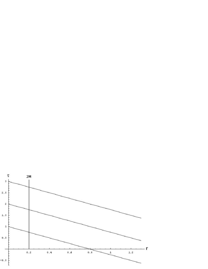
Figure 2.2: Radial Null geodesics reach and cross the event horizon at 2M without noticing it when defined with the affine parameter

2.2.2 General Null Geodesics and Critical Orbits

We will first solve Eqn. (2.25) in order to determine the the critical stable photon orbits. In order to do this we first consider the point of equilibrium and the associated impact parameter. This equilibrium point occurs when

$$\frac{du}{d\phi}=0$$ (2.33)

which means as the photon is orbiting the black hole $u$ does not change; so if the radial distance does not change it implies a circular orbit. Therefore we must solve

$$f(u)=\frac{1}{D^{2}}-u^{2}+2Mu^{3}=0$$ (2.34)

The sum and product of the roots $u_{1}$, $u_{2}$, and $u_{3}$ of this equation are given by

$$u_{1}+u_{2}+u_{3}=\frac{1}{2M}\qquad\textrm{and}\qquad u_{1}u_{2}u_{3}=-\frac{1}{2MD^{2}}$$ (2.35)

This shows that $f(u)=0$ must have a real negative root, and the two remaining roots can be real (distinct or coincident) or be a complex conjugate pair; however, the occurrence of coincident positive real roots implies the existence of a circular orbit. Thus, if a coincident root occurs it should be at the point given by the derivative of $f(u)$

$$f^{\prime}(u)=6Mu^{2}-2u=0$$ (2.36)

Which then has the solution $u_{1}=u_{2}=(3M)^{-1}$. For this solution the impact parameter of equation (2.34) is $D=(3\sqrt{3})M$. From the product condition, equation (2.35), we find that the roots of $f(u)=0$ are

$$u_{1}=u_{2}=\frac{1}{3M}\qquad\textrm{and}\qquad u_{3}=-\frac{1}{6M}\qquad\textrm{and}\qquad D=(3\sqrt{3})M$$ (2.37)

Therefore, when the impact parameter is $D=(3\sqrt{3})M$ then $\frac{du}{d\phi}$ vanishes for $u=(3M)^{-1}$, which implies a circular orbit of radius $3M$ is an allowed null geodesic [2].

Now we can consider a photon at $u=0$ with an impact parameter $D=(3\sqrt{3})M$. This, then, gives a trajectory of a photon spiralling in and tending to the critical orbit at $u=(3M)^{-1}$. The general differential equation for this impact parameter is given by rearranging and substituting for $D$ in Eqn. (2.25)

$$(\frac{du}{d\phi})^{2}=2M(u+\frac{1}{6M})(u-\frac{1}{3M})^{2}$$ (2.38)

From [2] we have the solution to this as

$$u=-\frac{1}{6M}+\frac{1}{2M}\tanh^{2}{\frac{1}{2}(\phi-\phi_{0})}$$ (2.39)

where $\phi_{0}$ is a constant of integration, given by:

$$\tanh^{2}{(-\frac{1}{2}\phi_{0})}=\frac{1}{3},$$ (2.40)

which gives: $u=0$ ($r\rightarrow\infty$) when $\phi=0$, and $u=\frac{1}{3M}$ when $\phi\rightarrow\infty$. Therefore a null geodesic arriving from infinity with an impact parameter $D=(3\sqrt{3})M$ approaches the circle of radius $3M$, asymptotically, by spiralling around it, as can be seen in Fig. 2.3. Also, numerically solving Eqn (2.26) we can show that as time increases $u$ tends to $\frac{1}{3M}$, which can be seen in Fig. 2.4.

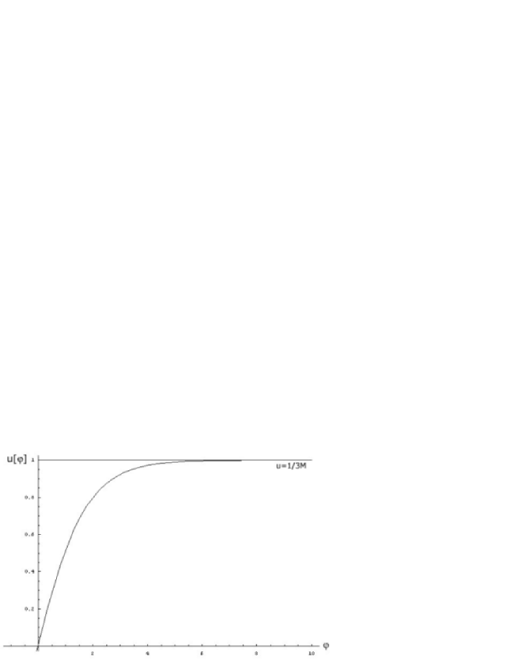
Figure 2.3: Null geodesic, with impact parameter $D=(3\sqrt{3})M$, arriving from infinity and approaching $u=\frac{1}{3M}$ asymptotically (M=1/3)

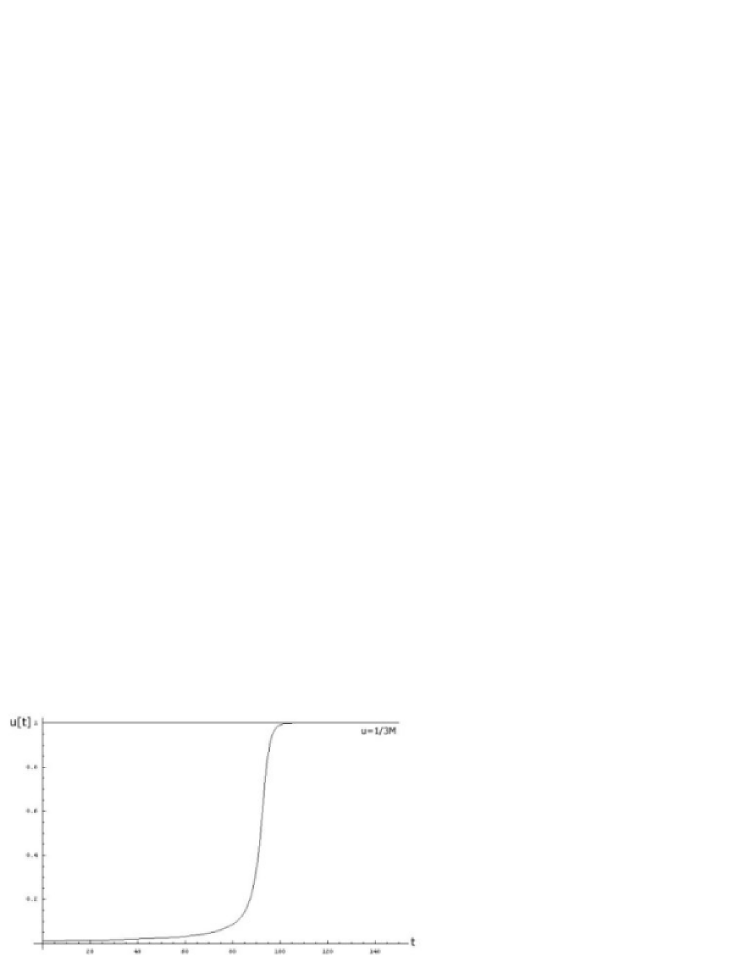
Figure 2.4: For impact parameter $D=(3\sqrt{3})M$ a null trajectory tends to $u=\frac{1}{3M}$ asymptotically with time.

Finally we can show that when an impact parameter other than $D=(3\sqrt{3})M$ is used, for example if we set $D=(3\sqrt{3})M-0.1$, the solution of Eqn. (2.25) shows that the photon falls past the critical orbit, through the event horizon, and into the singularity, Fig. 2.5. Using this new impact parameter in Eqn. (2.26) and, again solving numerically, we see that the photon comes in from infinity and tends to the event horizon, $u=\frac{1}{2M}$, asymptotically in time $t$, Fig. 2.6.

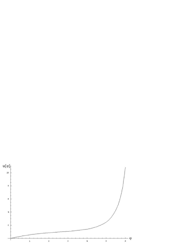
Figure 2.5: Null geodesic, with impact perimeter $D=(3\sqrt{3})M-0.1$, arrives from infinity and spirals into the singularity.

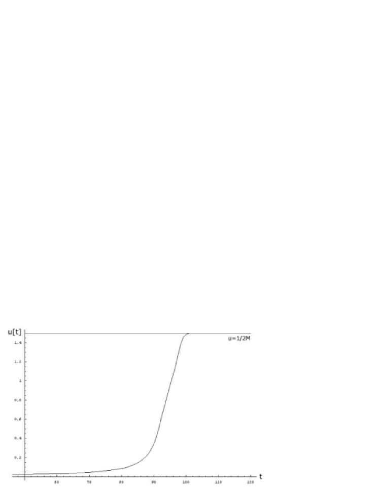
Figure 2.6: Null geodesic, with impact perimeter $D=(3\sqrt{3})M-0.1$, arrives from infinity and tends to $u=\frac{1}{2M}$ asymptotically in time $t$.

Chapter 3 Quantum Gravitational Optics

3.1 Photon Propagation in Curved Spacetime

Maxwell’s equations, in curved spacetime,

$$0=D_{\mu}F^{\mu\nu}$$ (3.1)

$$0 = D_{\mu}F_{\nu\lambda}+D_{\nu}F_{\lambda\mu}+D_{\lambda}F_{\mu\nu}$$ (3.2)

$$\Rightarrow F_{\mu\nu}=\partial_{\mu}A_{\nu}-\partial_{\nu}A_{\mu},$$ (3.3)

cannot be solved explicitly, and even in cases of extreme symmetry explicit solutions are difficult; this is due to the fact that as curved space acts as a dispersive material (i.e. bending light rays) plane wave solutions do not exist.

3.1.1 Geometric Optics in Curved Spacetime

In dispersive materials, where light rays are bent, we can consider the solution of Maxwell’s equations to be a simple perturbation of the plane wave solution. For example in curved space, relative to an observer, the electromagnetic waves can appear to be plane and monochromatic on a scale that is much larger compared to the typical wavelength, but very small compared with the typical radius of curvature of space time. Such "locally plane" waves can be represented, in geometric optics, by approximate solutions of Maxwell’s equations of the form[6]:

$$\mathcal{F}^{\mu\nu}=Re(F_{1}^{\mu\nu}+i\varepsilon F_{2}^{\mu\nu}+\ldots)e^{i\frac{\theta}{\varepsilon}}$$ (3.4)

and the electromagnetic field vector, defined by Eqn. (3.3), takes the form:

$$\mathcal{A}^{\mu}=Re(A_{1}^{\mu}+i\varepsilon A_{2}^{\mu}+\ldots)e^{i\frac{\theta}{\varepsilon}}$$ (3.5)

where the electromagnetic field is written as a slowly-varying amplitude and a rapidly-varying phase. The parameter $\varepsilon$ is introduced in order to keep track of the relative order of magnitude of terms, so in curved space Maxwell’s equations can be solved order-by-order in $\varepsilon$. In this formulation the wave vector is then defined as the gradient of the phase of the field, $k_{\mu}=D_{\mu}\frac{i}{\varepsilon}\theta=\partial_{\mu}\frac{i}{\varepsilon}\theta$, which in terms of the quantum interpretation is identified as the photon momentum. We can also write $A^{\mu}=Aa^{\mu}$, where $A$ represents the amplitude and $a_{\mu}$ (normalized as $a_{\mu}a^{\mu}=-1$) specifies the wave polarization. These vectors then satisfy the condition $k_{\mu}a^{\mu}=0$.

Geometric Optics and Null Dynamics

In this notation Eqn. (3.1) can be written, to leading order $\mathcal{O}(\frac{1}{\varepsilon})$, as:

$$\partial_{\mu}(F_{1}^{\mu\nu}e^{i\frac{\theta}{\varepsilon}}) = F_{1}^{\mu\nu}e^{i\frac{\theta}{\varepsilon}}(\frac{i}{\varepsilon}\partial_{\mu}\theta)$$

$$\Rightarrow\qquad k_{\mu}F_{1}^{\mu\nu} = 0$$ (3.6)

and Eqn. (3.3) becomes:

$$F_{1\mu\nu}e^{i\frac{\theta}{\varepsilon}} = (\partial_{\mu}A_{1\nu}-\partial_{\nu}A_{1\mu})e^{i\frac{\theta}{\varepsilon}}$$

$$= \frac{i}{\varepsilon}(\partial_{\mu}\theta A_{1\nu}-\partial_{\nu}\theta A_{1\mu})e^{i\frac{\theta}{\varepsilon}}$$

$$\Rightarrow\qquad F_{1\mu\nu} = k_{\mu}A_{1\nu}-k_{\nu}A_{1\mu}$$ (3.7)

Now, by combining these, we have:

$$k_{\mu}F_{1}^{\mu\nu} = k_{\mu}(k^{\mu}A_{1}^{\nu}-k^{\nu}A_{1}^{\mu})=0$$

$$= (k_{\mu}k^{\mu})A_{1}^{\nu}-k^{\nu}(k_{\mu}A_{1}^{\mu})$$

$$\Rightarrow\qquad k^{2}a^{\nu} = 0$$ (3.8)

and from this we can deduce that $k^{2}=0$, i.e. $k^{\mu}$ is a null vector. Also, it follows from the definition of $k^{\mu}$ as a gradient that $D_{\mu}k_{\nu}=D_{\nu}k_{\mu}$, so

$$k^{\mu}D_{\mu}k^{\nu}=k^{\mu}D^{\nu}k_{\mu}=\frac{1}{2}D^{\nu}k^{2}=0$$ (3.9)

Using this, and the fact that light rays are defined as the curves given by $x_{\mu}(s)$ where $\frac{dx_{\mu}}{ds}=k_{\mu}$, we can derive the geodesic equation as follows[7]:

$$0 = k^{\mu}D_{\mu}k^{\nu}$$ (3.10)

$$= \frac{d^{2}x^{\nu}}{ds^{2}}+\Gamma^{\nu}_{\mu\lambda}\frac{dx^{\mu}}{ds}\frac{dx^{\lambda}}{ds}$$

3.2 Quantum Modified Null Dynamics

As was seen in Sec. 1.2, using the effective action, Eqn. (1.4), the equation of motion becomes:

$$0=D_{\mu}F^{\mu\nu}-\frac{1}{m^{2}}[2bR_{\mu\lambda}D^{\mu}F^{\lambda\nu}+4cg^{\nu\tau}R_{\mu\tau\lambda\rho}D^{\mu}F^{\lambda\rho}]$$ (3.11)

and the Bianchi identity, Eqn. (3.2), remains unchanged. Now, as before we can determine the quantum modified light cone and geodesic equations.

Quantum Modified Light Cone

Substituting Eqn. (3.4) in (3.11) we find, again to $\mathcal{O}(\frac{1}{\varepsilon})$:

$$0=\frac{i}{\varepsilon}(D_{\mu}\theta)e^{i\frac{\theta}{\varepsilon}}F_{1}^{\mu\nu} - \frac{1}{m^{2}}[2bR_{\mu\lambda}\frac{i}{\varepsilon}(D^{\mu}\theta)e^{i\frac{\theta}{\varepsilon}}F_{1}^{\lambda\nu}$$

$$+ 4cg^{\nu\tau}R_{\mu\tau\lambda\rho}\frac{i}{\varepsilon}(D^{\mu}\theta)e^{i\frac{\theta}{\varepsilon}}F_{1}^{\lambda\rho}]$$

$$\Rightarrow\qquad 0=k_{\mu}F_{1}^{\mu\nu}-\frac{1}{m_{e}^{2}}[2bR_{\mu\lambda}k^{\mu}F_{1}^{\lambda\nu}+4cg^{\nu\tau}R_{\mu\tau\lambda\rho}k^{\mu}F_{1}^{\lambda\rho}]$$ (3.12)

and using Eqn. (3.7) we have:

$$0=k_{\mu}(k^{\mu}A_{1}^{\nu}-k^{\nu}A_{1}^{\mu}) - \frac{1}{m_{e}^{2}}[2bR_{\mu\lambda}k^{\mu}(k^{\lambda}A_{1}^{\nu}-k^{\nu}A_{1}^{\lambda})$$

$$+ 4cg^{\nu\tau}R_{\mu\tau\lambda\rho}k^{\mu}(k^{\lambda}A_{1}^{\rho}-k^{\rho}A_{1}^{\lambda})]$$

using $k_{\mu}A^{\mu}=0$ this becomes:

$$0=k_{\mu}k^{\mu}A_{1}^{\nu} - \frac{1}{m_{e}^{2}}[2bR_{\mu\lambda}k^{\mu}(k^{\lambda}A_{1}^{\nu}-k^{\nu}A_{1}^{\lambda})$$ (3.13)

$$+ 4cg^{\nu\tau}R_{\mu\tau\lambda\rho}k^{\mu}(2k^{\lambda}A_{1}^{\rho})]$$

where $A_{1}^{\nu}=A_{1}a^{\nu}$, and the last line is simplified by relabeling of indices. Now, Contracting with $Aa_{\nu}$ and eliminating $A$ we have:

$$0=-k_{\mu}k^{\mu}+\frac{2b}{m_{e}^{2}}R_{\mu\lambda}k^{\mu}k^{\lambda}-\frac{8c}{m_{e}^{2}}R_{\mu\tau\lambda\rho}k^{\mu}k^{\lambda}a_{1}^{\tau}a_{1}^{\rho}$$

This then gives the quantum modified light cone:

$$k^{2}-\frac{2b}{m^{2}}R_{\mu\lambda}k^{\mu}k^{\lambda}-\frac{8c_{\alpha}}{m_{e}^{2}}R_{\mu\tau\lambda\rho}k^{\mu}k^{\lambda}a^{\tau}a^{\rho}=k^{2}-\delta k(a)=0$$ (3.14)

where we have replaced the constant $c=-\frac{\alpha}{360\pi}$ with $c_{\alpha}=\frac{\alpha}{360\pi}$ for convenience of interpretation, i.e. the sign of the light cone is immediately obvious from $R_{\mu\tau\lambda\rho}k^{\mu}k^{\lambda}a^{\tau}a^{\rho}$. As we will be working in the Schwarzschild spacetime the quantum modified light cone for the Ricci flat case ($R_{\mu\lambda}=0$) is given by:

$$k^{2}=\frac{8c_{\alpha}}{m_{e}^{2}}R_{\mu\tau\lambda\rho}k^{\mu}k^{\lambda}a^{\tau}a^{\rho}=\delta k(a)$$ (3.15)

Here the sign of the light cone depends on polarization and the photon trajectory; if the correction is positive we have space-like motion, and if it’s negative we have time-like motion.

Quantum Modified Geodesic Equation

The photon trajectories corresponding to the quantum modified equation of motion, (3.11), can be represented by a generalised version of Eqn. (3.9):

$$0 = \frac{1}{2}D_{\nu}[k^{2}-\frac{2b}{m^{2}}R_{\mu\lambda}k^{\mu}k^{\lambda}-\frac{8c_{\alpha}}{m_{e}^{2}}R_{\mu\tau\lambda\rho}k^{\mu}k^{\lambda}a^{\tau}a^{\rho}]$$

$$0 = \frac{1}{2}D_{\nu}k^{2}-\frac{1}{m^{2}}D_{\nu}[bR_{\mu\lambda}k^{\mu}k^{\lambda}+4c_{\alpha}R_{\mu\tau\lambda\rho}k^{\mu}k^{\lambda}a^{\tau}a^{\rho}]$$

$$\Rightarrow\qquad 0 = \frac{d^{2}x^{\nu}}{ds^{2}}+\Gamma_{\mu\lambda}^{\nu}\frac{dx^{\mu}}{ds}\frac{dx^{\lambda}}{ds}$$ (3.16)

$$- \frac{1}{m^{2}}\partial_{\nu}[(bR_{\beta\gamma}+4c_{\alpha}R_{\beta\sigma\gamma\tau}a^{\sigma}a^{\tau})\frac{dx^{\beta}}{ds}\frac{dx^{\gamma}}{ds}]$$

where we have used $k^{\mu}=\frac{dx^{\mu}}{ds}$, and covariant derivative in the second term is replaced by a partial derivative as it’s acting on a scalar. In Ricci spacetime this equation becomes:

$$0=\frac{d^{2}x^{\nu}}{ds^{2}}+\Gamma_{\mu\lambda}^{\nu}\frac{dx^{\mu}}{ds}\frac{dx^{\lambda}}{ds}-\frac{4c_{\alpha}}{m^{2}}\partial_{\nu}[R_{\beta\sigma\gamma\tau}a^{\sigma}a^{\tau}\frac{dx^{\beta}}{ds}\frac{dx^{\gamma}}{ds}]$$ (3.17)

3.3 Horizon Theorem and Polarization Rule

There are two general features associated with quantum modified photon propagation[7]. First, it is a general result that the velocity of radially directed photons remains equal to $c$ at the event horizon. Second, for Ricci flat spacetimes (such as Schwarzschild[1] and Kerr[8] spacetimes), the velocity shifts for the two transverse polarizations are always equal and opposite. However, this is no longer true for non-Ricci flat cases (such as Robertson-Walker spacetime[1]). In these cases, the polarization averaged velocity shift is proportional to the matter energy-momentum tensor. These features can be easily shown by using the Newman-Penrose formalism: this characterises spacetimes using a set of complex scalars, which are found by contracting the Weyl tensor with elements of a null tetrad[2].

Newman-Penrose Formalism

We choose the basis vectors of the null tetrad as[7]: $l^{\mu}=k^{\mu}$, the photon momentum. Then, we denote the two spacelike, normalized, transverse polarization vectors by $a^{\mu}$ and $b^{\mu}$ and construct the null vectors $m^{\mu}=\frac{1}{\sqrt{2}}(a^{\mu}+ib^{\mu})$ and $\bar{m}^{\mu}=\frac{1}{\sqrt{2}}(a^{\mu}-ib^{\mu})$. We complete the tetrad with a further null vector $n^{\mu}$, which is orthogonal to $m^{\mu}$ and $\bar{m}^{\mu}$. We then have the conditions:

$$l\cdot m=l\cdot\bar{m}=n\cdot m=n\cdot\bar{m}=0$$ (3.18)

from orthogonality, and:

$$l\cdot l=n\cdot n=m\cdot m=\bar{m}\cdot\bar{m}=0$$ (3.19)

since the basis vectors are null. Finally, we impose:

$$l\cdot n=-m\cdot\bar{m}=1$$ (3.20)

The Weyl tensor, given in terms of the Riemann and Ricci tensors, is:

$$C_{\mu\nu\gamma\delta}=R_{\mu\nu\gamma\delta} - \frac{1}{2}(\eta_{\mu\gamma}R_{\nu\delta}-\eta_{\nu\gamma}R_{\mu\delta}-\eta_{\mu\delta}R_{\nu\gamma}+\eta_{\nu\delta}R_{\mu\gamma})$$ (3.21)

$$+ \frac{1}{6}(\eta_{\mu\gamma}\eta_{\nu\delta}-\eta_{\mu\delta}\eta_{\nu\gamma})R$$

where $R_{\mu\gamma}=\eta^{\nu\delta}R_{\mu\nu\gamma\delta}$ and $R=\eta^{\mu\nu}R_{\mu\nu}$; and the Weyl tensor satisfies the trace-free condiation:

$$\eta^{\mu\delta}C_{\mu\nu\gamma\delta}=0$$ (3.22)

and the cyclicity property:

$$C_{1234}+C_{1342}+C_{1423}=0$$ (3.23)

Now, using the null tetrad, we can denote the ten independent components of the Weyl tensor by the five complex Newman-Penrose scalars:

$$\Psi_{0} = -C_{\mu\nu\gamma\delta}l^{\mu}m^{\nu}l^{\gamma}m^{\delta}$$

$$\Psi_{1} = -C_{\mu\nu\gamma\delta}l^{\mu}n^{\nu}l^{\gamma}m^{\delta}$$

$$\Psi_{2} = -C_{\mu\nu\gamma\delta}l^{\mu}m^{\nu}\bar{m}^{\gamma}n^{\delta}$$

$$\Psi_{3} = -C_{\mu\nu\gamma\delta}l^{\mu}n^{\nu}\bar{m}^{\gamma}n^{\delta}$$

$$\Psi_{4} = -C_{\mu\nu\gamma\delta}n^{\mu}\bar{m}^{\nu}n^{\gamma}\bar{m}^{\delta}$$ (3.24)

3.3.1 Polarization Sum Rule

Ricci Flat Spacetime

In Ricci flat spacetime, summing the quantum correction over the two polarizations leads to the following polarization sum rule:

$$\sum_{a}\delta k(a)=0$$ (3.25)

This can be proven by suming the quantum correction in Eqn. (3.15) over the two polarizations,

$$\sum_{a}\delta k(a)=\frac{8c_{\alpha}}{m_{e}^{2}}\sum_{a}R_{\mu\nu\gamma\delta}k^{\mu}k^{\gamma}a^{\nu}a^{\delta}$$ (3.26)

In the Newman-Penrose basis, using $k=l$, $a=\frac{\sqrt{2}}{2}(m+\bar{m})$, $b=-\frac{i\sqrt{2}}{2}(m-\bar{m})$, and the fact that $C_{\mu\nu\gamma\delta}=R_{\mu\nu\gamma\delta}$ for the Ricci flat case, we have:

$$\sum_{a}R_{\mu\nu\gamma\delta}k^{\mu}k^{\gamma}a^{\nu}a^{\delta} = \frac{1}{2}C_{\mu\nu\gamma\delta}l^{\mu}l^{\gamma}(m^{\nu}+\bar{m}^{\nu})(m^{\delta}+\bar{m}^{\delta})$$ (3.27)

$$- \frac{1}{2}C_{\mu\nu\gamma\delta}l^{\mu}l^{\gamma}(m^{\nu}-\bar{m}^{\nu})(m^{\delta}-\bar{m}^{\delta})$$

$$= C_{\mu\nu\gamma\delta}l^{\mu}l^{\gamma}(m^{\nu}\bar{m}^{\delta}+\bar{m}^{\nu}m^{\delta})$$

This particular contraction is equal to zero as it’s not part of the complex scalars in Eqns. (3.24); hence the sum of the two quantum corrections is zero. This implies the trajectory (and velocity) shifts are equal and opposite.

Non-Ricci Flat Spacetime

For the non-Ricci flat spacetimes the polarization sum rule is given as:

$$\sum_{a}\delta k(a)=-\frac{8\pi}{m_{e}^{2}}(2b-8c_{\alpha})T_{\mu\nu}k^{\mu}k^{\nu}$$ (3.28)

where $T_{\mu\nu}$ is the energy-momentum tensor. This can be shown by proceeding as before, but now we include the Ricci tensor and scalar, as in Eqn. (3.21):

$$\sum_{a}R_{\mu\nu\gamma\delta}k^{\mu}k^{\gamma}a^{\nu}a^{\delta}=C_{\mu\nu\gamma\delta}l^{\mu}l^{\gamma}(m^{\nu}\bar{m}^{\delta}+\bar{m}^{\nu}m^{\delta})-R_{\mu\gamma}l^{\mu}l^{\gamma}$$ (3.29)

As before the first term on the RHS is zero, and the second term is only dependent on the photon momentum. Then, combining this with the Ricci term in Eqn. (3.14) we have:

$$\sum_{a}\delta k(a)=\frac{1}{m_{e}^{2}}(2b-8c_{\alpha})R_{\mu\nu}k^{\mu}k^{\nu}$$ (3.30)

Finally replacing the Ricci tensor with the energy-momentum tensor, by using the Einstein equation

$$R_{\mu\nu}=-8\pi T_{\mu\nu}+\frac{1}{2}Rg_{\mu\nu}$$ (3.31)

we obtain Eqn. (3.28).

3.3.2 Horizon Theorem

At the event horizon, photons with momentum directed normal to the horizon have velocity equal to $c$, i.e. the light cone remains $k^{2}=0$, independent of polarization[7].

This can be easily proven for the Ricci flat spacetime, using the orthonormal vectors $k^{a}=(E_{k},E_{k},0,0)$, $a^{b}=(0,0,1,0)$ and $a^{b}=(0,0,0,1)$. Therefore, using these vectors in Eqn. (3.15), we have:

$$k^{2}=\frac{8c_{\alpha}}{m_{e}^{2}}R_{abcd}k^{a}k^{c}a^{b}a^{d}=0$$ (3.32)

So, in Ricci flat spacetime all radially projected photon trajectories remain unchanged.

It is also possible to prove the horizon theorem for the general case (for Ricci and non-Ricci flat spacetimes) that the light cone at the event horizon is unchanged. This can be seen in the null tetrad, so that the physical, space-like, polarization vectors $a^{\mu}$ and $b^{\mu}$ lie parallel to the event horizon 2-surface, while $k^{\mu}$ is the null vector normal to the surface. Then, from Eqn. (3.14) we have for the two polarizations:

$$k^{2} = \frac{2b}{m_{e}^{2}}R_{\mu\gamma}k^{\mu}k^{\gamma}+\frac{8c_{\alpha}}{m_{e}^{2}}R_{\mu\nu\gamma\delta}k^{\mu}k^{\gamma}a^{\nu}a^{\delta}$$ (3.33)

$$= \frac{2b}{m_{e}^{2}}R_{\mu\gamma}l^{\mu}l^{\gamma}+\frac{8c_{\alpha}}{m_{e}^{2}}[-\frac{1}{2}R_{\mu\gamma}l^{\mu}l^{\gamma}\pm C_{\mu\nu\gamma\delta}l^{\mu}l^{\gamma}\frac{1}{2}(m^{\nu}\pm\bar{m}^{\nu})(m^{\delta}\pm\bar{m}^{\delta})]$$

$$= \frac{1}{m_{e}^{2}}(2b-4c_{\alpha})R_{\mu\gamma}l^{\mu}l^{\gamma}\pm\frac{4c_{\alpha}}{m_{e}^{2}}C_{\mu\nu\gamma\delta}l^{\mu}l^{\gamma}\frac{1}{2}(m^{\nu}\pm\bar{m}^{\nu})(m^{\delta}\pm\bar{m}^{\delta})$$

Using Eqn. (3.31) and the fact that $C_{\mu\nu\gamma\delta}l^{\mu}l^{\gamma}(m^{\nu}\bar{m}^{\delta}+\bar{m}^{\nu}m^{\delta})=0$, we can write this as:

$$k^{2} = -\frac{8\pi}{m_{e}^{2}}(2b-4c_{\alpha})T_{\mu\gamma}l^{\mu}l^{\gamma}\pm\frac{4c_{\alpha}}{m_{e}^{2}}C_{\mu\nu\gamma\delta}l^{\mu}l^{\gamma}(m^{\nu}m^{\delta}+\bar{m}^{\nu}\bar{m}^{\delta})$$ (3.34)

and in terms of the Newman-Penrose scalars this can be written as:

$$k^{2} = -\frac{8\pi}{m_{e}^{2}}(2b-4c_{\alpha})T_{\mu\gamma}l^{\mu}l^{\gamma}\pm\frac{8c_{\alpha}}{m_{e}^{2}}\Psi_{0},$$ (3.35)

where the simplification in the last term on the RHS is possible as $\Psi_{0}$ is real for Schwarzschild spacetime. In general Eqn. (3.35) is non zero, however, at the event horizon the terms: $T_{\mu\gamma}l^{\mu}l^{\gamma}$ and $\Psi_{0}$ are zero for stationary spacetimes[7, 9].

Physically the Ricci term represents the flow of matter across the horizon and the Weyl term represents the flow of gravitational radiation[7], and both are zero in classic general relativity; and as, even with the quantum modification, the light cone remains unchanged at the event horizon, means the event horizon is fixed and light cannot escape from inside the black hole.

Chapter 4 Quantum Modified Trajectories

In this chapter we will analyse how the classical null trajectories, described in Chapter 2, are modified in Schwarzschild spacetime, due to quantum modifications of the equations of motion of general relativity. Using Eqn. (3.14) we will calculate the quantum corrected version of Eqn. (2.25), which will then describe the quantum modified motion of a null trajectory in a Schwarzschild spacetime. Using this, and following the methods of Chapter 2, we will begin by studying simple critical circular orbits at the stationary point, $u=1/3M$. As stated in the polarization rule, the critical orbit should be shifted up and down by equal amounts, depending on the polarization of each photon. Also, we will show that these modifications are only valid if the "classic" impact parameter corresponding to the stationary orbit is adjusted, depending on the photon’s polarization, in order to compensate for the orbit shift. This information, of the modified orbits and the corresponding impact parameter for each polarization, will then be used to determine the general trajectory of a (vertically or horizontally polarized) photon coming in from infinity and tending to one of the two shifted critical orbits. We will then go on to show that these quantum modifications have no effect on the event horizon, that is, when the impact parameter is accordingly adjusted and a photon falls into the singularity the event horizon remains fixed at $u=1/2M$.

4.1 Quantum Modified Circular Orbits

In Schwarzschild spacetime, using $k^{\nu}=dx^{\nu}/d\tau$, Eqn. (3.15) can be written as:

$$0 = \dot{r}^{2}-(1-\frac{2M}{r})^{2}\dot{t}^{2}+r^{2}(1-\frac{2M}{r})\dot{\theta}^{2}$$ (4.1)

$$+ (1-\frac{2M}{r})r^{2}\dot{\phi}^{2}+\frac{8c_{\alpha}}{m_{e}^{2}}(1-\frac{2M}{r})R_{\mu\nu\gamma\delta}k^{\mu}k^{\gamma}a^{\nu}a^{\delta}$$

and Eqn. (3.17) as:

$$0 = \ddot{t}+\frac{2M}{r^{2}}(1-\frac{2M}{r})^{-1}\dot{r}\dot{t}$$ (4.2)

$$- \frac{4c_{\alpha}}{m_{e}^{2}}\partial_{t}(R_{\mu\nu\gamma\delta}a^{\nu}a^{\delta}\frac{dx^{\mu}}{d\tau}\frac{dx^{\gamma}}{d\tau})$$

$$0 = \ddot{r}-\frac{M}{r^{2}}(1-\frac{2M}{r})^{-1}\dot{r}^{2}-r(1-\frac{2M}{r})\dot{\phi}^{2}$$ (4.3)

$$+ \frac{M}{r^{2}}(1-\frac{2M}{r})\dot{t}^{2}-\frac{4c_{\alpha}}{m_{e}^{2}}\partial_{r}(R_{\mu\nu\gamma\delta}a^{\nu}a^{\delta}\frac{dx^{\mu}}{d\tau}\frac{dx^{\gamma}}{d\tau})$$

$$0 = \ddot{\phi}+\frac{2\dot{r}\dot{\phi}}{r}-\frac{4c_{\alpha}}{m_{e}^{2}}\partial_{\phi}(R_{\mu\nu\gamma\delta}a^{\nu}a^{\delta}\frac{dx^{\mu}}{d\tau}\frac{dx^{\gamma}}{d\tau})$$ (4.4)

$$0 = -\frac{4c_{\alpha}}{m_{e}^{2}}\partial_{\theta}(R_{\mu\nu\gamma\delta}a^{\nu}a^{\delta}\frac{dx^{\mu}}{d\tau}\frac{dx^{\gamma}}{d\tau})$$ (4.5)

where $c_{\alpha}=\frac{\alpha}{360\pi}$. Now, in order to consider quantum modified circular orbits we require three things: (i) the Riemann tensor components, (ii) the photon wave vectors, $k^{\mu}=\frac{dx^{\mu}}{d\tau}$, for circular orbits, and finally (iii) the photon polarization vectors, $a^{\mu}$. Due to the circular nature of the orbit the simplest basis to work in is the orthonormal basis. In this frame the required polarization and wave vectors, for circular orbits, are simply given as:

$$a^{\mu}=(0,1,0,0)\qquad\textrm{Planar Polarized}$$ (4.6)

$$a^{\mu}=(0,0,1,0)\qquad\textrm{Vertically Polarized}$$ (4.7)

$$k^{\mu}=\frac{dx^{\mu}}{d\tau}=(E_{k},0,0,E_{k})\qquad\textrm{$4$-momentum along $\phi$}$$ (4.8)

Now using these photon vectors, the quantum modifications in Eqns. (4.1)-(4.5), can be expanded to give:

• For the planar polarized case we have:

  $$R_{abcd}k^{a}k^{c}a^{b}a^{d} = R_{arcr}k^{a}k^{c}=E_{k}^{2}(R_{arcr}\hat{k}^{a}\hat{k}^{c})$$ (4.9)

  $$= E_{k}^{2}(R_{trtr}+R_{\phi r\phi r}+2R_{tr\phi r})$$

• For the vertically polarized case we have:

  $$R_{abcd}k^{a}k^{c}a^{b}a^{d} = R_{a\theta c\theta}k^{a}k^{c}=E_{k}^{2}(R_{a\theta c\theta}\hat{k}^{a}\hat{k}^{c})$$ (4.10)

  $$= E_{k}^{2}(R_{t\theta t\theta}+R_{\phi\theta\phi\theta})$$

Using the six independent components of the Riemann tensor in the orthonormal basis, we find:

$$R_{trrt}=-R_{trtr}=-\frac{2M}{r^{3}}\Rightarrow R_{trtr}=\frac{2M}{r^{3}}$$ (4.11)

$$R_{\phi rr\phi}=-R_{\phi r\phi r}=-\frac{M}{r^{3}}\Rightarrow R_{\phi r\phi r}=\frac{M}{r^{3}}$$ (4.12)

$$R_{\theta t\theta t}=R_{t\theta t\theta}=-\frac{M}{r^{3}}\Rightarrow R_{t\theta t\theta}=-\frac{M}{r^{3}}$$ (4.13)

$$R_{\phi\theta\theta\phi}=-R_{\phi\theta\phi\theta}=\frac{2M}{r^{3}}\Rightarrow R_{\phi\theta\phi\theta}=-\frac{2M}{r^{3}}$$ (4.14)

$$R_{tr\phi r}=0$$ (4.15)

Then Eqns. (4.9) and (4.10) become:

• For the planar polarized case:

  $$R_{abcd}k^{a}k^{c}a^{b}a^{d}=E_{k}^{2}(R_{trtr}+R_{\phi r\phi r}+2R_{tr\phi r})=\frac{3E_{k}^{2}M}{r^{3}}$$ (4.16)

  with the relevant derivatives:

  $$\partial_{t}\frac{3E_{k}^{2}M}{r^{3}} = 0\qquad\partial_{r}\frac{3E_{k}^{2}M}{r^{3}}=-\frac{9E_{k}^{2}M}{r^{4}}$$

  $$\partial_{\theta}\frac{3E_{k}^{2}M}{r^{3}} = 0\qquad\partial_{\phi}\frac{3E_{k}^{2}M}{r^{3}}=0$$ (4.17)

• For the vertically polarized case:

  $$R_{abcd}k^{a}k^{c}a^{b}a^{d}=E_{k}^{2}(R_{t\theta t\theta}+R_{\phi\theta\phi\theta})=-\frac{3E_{k}^{2}M}{r^{3}}$$ (4.18)

  and the relevant derivatives:

  $$-\partial_{t}\frac{3E_{k}^{2}M}{r^{3}} = 0\qquad-\partial_{r}\frac{3E_{k}^{2}M}{r^{3}}=\frac{9E_{k}^{2}M}{r^{4}}$$

  $$-\partial_{\theta}\frac{3E_{k}^{2}M}{r^{3}} = 0\qquad-\partial_{\phi}\frac{3E_{k}^{2}M}{r^{3}}=0$$ (4.19)

From Eqns. (3.15), (4.16) and (4.18) we can see that:

$$k^{2} \sim \frac{3E_{k}^{2}M}{r^{3}}\qquad\textrm{For Planar Polarization}$$ (4.20)

$$k^{2} \sim -\frac{3E_{k}^{2}M}{r^{3}}\qquad\textrm{For Vertical Polarization}$$ (4.21)

This implies that, as the light cone for planar polarization is positive, it represents a photon trajectory with a speed $<c$, and as the light cone for vertical polarization is negative, it represents a photon trajectory with a speed $>c$.

Planar Polarization

Considering the planar polarized case first, we can use Eqns. (4.16) and (4.17) to rewrite Eqns. (4.1)-(4.4) as:

$$0 = \dot{r}^{2}-(1-\frac{2M}{r})^{2}\dot{t}^{2}+r^{2}(1-\frac{2M}{r})\dot{\theta}^{2}$$ (4.22)

$$+ (1-\frac{2M}{r})r^{2}\dot{\phi}^{2}+\frac{8c_{\alpha}}{m_{e}^{2}}(1-\frac{2M}{r})\frac{3E_{k}^{2}M}{r^{3}}$$

$$0 = \ddot{t}+\frac{2M}{r^{2}}(1-\frac{2M}{r})^{-1}\dot{r}\dot{t}$$ (4.23)

$$0 = \ddot{r}-\frac{M}{r^{2}}(1-\frac{2M}{r})^{-1}\dot{r}^{2}-r(1-\frac{2M}{r})\dot{\phi}^{2}$$ (4.24)

$$+ \frac{M}{r^{2}}(1-\frac{2M}{r})\dot{t}^{2}+\frac{4c_{\alpha}}{m_{e}^{2}}\frac{9E_{k}^{2}M}{r^{4}}$$

$$0 = \ddot{\phi}+\frac{2\dot{r}\dot{\phi}}{r}$$ (4.25)

where Eqn. (4.5) becomes zero. Now, using the solutions of (4.23) and (4.25), as given by (2.12) and (2.13), we can rewrite Eqn. (4.22) as a simple quantum modified trajectory equation for circular orbits with radius $r$ and in a plane $\theta=\frac{\pi}{2}$:

$$0 = \dot{r}^{2}-E^{2}+(1-\frac{2M}{r})\frac{J^{2}}{r^{2}}+\frac{8c_{\alpha}}{m_{e}^{2}}(1-\frac{2M}{r})\frac{3E_{k}^{2}M}{r^{3}}$$

$$\Rightarrow\qquad E^{2} = (\frac{dr}{d\tau})^{2}+(1-\frac{2M}{r})(\frac{24cE_{k}^{2}M}{m_{e}^{2}r^{3}}+\frac{J^{2}}{r^{2}})$$ (4.26)

To make this equation more meaningful and easier to solve we make the following transformations:

$$\tau\rightarrow\phi\qquad\frac{dr}{d\phi}\cdot\frac{d\phi}{d\tau}=\frac{dr}{d\phi}\cdot\frac{J}{r^{2}}$$ (4.27)

$$r\rightarrow u=\frac{1}{r}\qquad\frac{du}{d\phi}\cdot\frac{dr}{du}=\frac{du}{d\phi}\cdot(-\frac{1}{u^{2}})$$ (4.28)

Therefore, Eqn. (4.26) becomes:

$$E^{2} = (\frac{dr}{d\phi})^{2}\cdot(\frac{J}{r^{2}})^{2}+(1-\frac{2M}{r})(\frac{24c_{\alpha}E_{k}^{2}M}{m_{e}^{2}r^{3}}+\frac{J^{2}}{r^{2}})$$ (4.29)

$$= (\frac{du}{d\phi})^{2}\cdot(-\frac{1}{u^{2}})^{2}\cdot(Ju^{2})^{2}+(1-2Mu)(\frac{24c_{\alpha}E_{k}^{2}Mu^{3}}{m_{e}^{2}}+J^{2}u^{2})$$

$$= (\frac{du}{d\phi})^{2}\cdot J^{2}+(1-2Mu)(\frac{24c_{\alpha}E_{k}^{2}Mu^{3}}{m_{e}^{2}}+J^{2}u^{2})$$

Which can be written as:

$$(\frac{du}{d\phi})^{2} = 2M^{2}Au^{4}+(2M-MA)u^{3}-u^{2}+\frac{E^{2}}{J^{2}}$$ (4.30)

where we have defined the dimensionless constant:

$$A=\frac{24c_{\alpha}E_{k}^{2}}{J^{2}m_{e}^{2}}=\frac{72c_{\alpha}}{m_{e}^{2}D^{2}},$$ (4.31)

In the last form we have used (without proof) the relation $E_{k}=\sqrt{3}E$, which will be proven in Sec. 4.2.1, Eqn. (4.68).

Vertical Polarization

Similarly, for the vertically polarized case, using Eqns. (4.18) and (4.19) in Eqns. (4.1)-(4.5) to give:

$$0 = \dot{r}^{2}-(1-\frac{2M}{r})^{2}\dot{t}^{2}+r^{2}(1-\frac{2M}{r})\dot{\theta}^{2}$$ (4.32)

$$+ (1-\frac{2M}{r})r^{2}\dot{\phi}^{2}-\frac{8c_{\alpha}}{m_{e}^{2}}(1-\frac{2M}{r})\frac{3E_{k}^{2}M}{r^{3}}$$

$$0 = \ddot{t}+\frac{2M}{r^{2}}(1-\frac{2M}{r})^{-1}\dot{r}\dot{t}$$ (4.33)

$$0 = \ddot{r}-\frac{M}{r^{2}}(1-\frac{2M}{r})^{-1}\dot{r}^{2}-r(1-\frac{2M}{r})\dot{\phi}^{2}$$ (4.34)

$$+ \frac{M}{r^{2}}(1-\frac{2M}{r})\dot{t}^{2}-\frac{4c_{\alpha}}{m_{e}^{2}}\frac{9E_{k}^{2}M}{r^{4}}$$

$$0 = \ddot{\phi}+\frac{2\dot{r}\dot{\phi}}{r}$$ (4.35)

which, in a similar way as before, gives us the equation of motion for the vertically polarized photon:

$$(\frac{du}{d\phi})^{2}=-2M^{2}Au^{4}+(2M+MA)u^{3}-u^{2}+\frac{E^{2}}{J^{2}}$$ (4.36)

4.1.1 Quantum Modified Critical Orbits

Now the general equation for the quantum modified circular orbits is:

$$(\frac{du}{d\phi})^{2}=\pm AM(2Mu-1)u^{3}+2Mu^{3}-u^{2}+\frac{1}{D^{2}}=f(u)$$ (4.37)

where $+$ is for planar polarization in the $r$ direction, $-$ is for vertical polarization in the $\theta$ direction and $D$ is the impact parameter. As $A\rightarrow 0$ Eqn. (4.37) tends to the classic orbit equation in general relativity, Eqns. (2.25). Therefore, in order to determine the magnitude of the quantum correction we can calculate the order of $A$ using typical values for $m_{e}$, $D$ and $c_{\alpha}$, in Eqn. (4.31). Using $m_{e}c/h\sim 10^{11}$ for the electron mass (as it is given as inverse length), $c_{\alpha}=\alpha/360\pi\sim 10^{-6}$, and the mass of the sun inserted into the critical impact parameter: $D=3\sqrt{3}GM_{\bigodot}/c^{2}\sim 10^{2}$ (given in terms of length), this then gives us:

$$A=\frac{72c_{\alpha}}{m_{e}^{2}D^{2}}\sim\frac{10^{-6}}{(10^{11}10^{2})^{2}}\sim 10^{-32}$$ (4.38)

With the order of $A$ being so small the correction in Eqn. (4.37) will be tiny compared to the size of the orbit ($r=3GM/c^{2}\sim 10^{2}$); therefore the modified orbits will not differ from the classic critical orbit, given by Eqn. (2.25), by very much.

We will now determine the quantum modified critical circular orbits. In order to solve Eqn. (4.37), we can use the fact, from the polarization rule, that the modified orbits should be shifted above and below $u=\frac{1}{3M}$ by equal amounts depending on polarization. So we expect a solution of the type $u=\frac{1}{3M}\pm\delta u$; which means we can try a simple modified solution of the form:

$$u=u_{0}+ku_{1}$$ (4.39)

where $u_{0}=\frac{1}{3M}$, $u_{1}$ is the quantum modification, and $k$ is a small constant depending on the quantum modification $A$.

Planar Polarized Critical Orbit

Working with Planar polarization, we can substitute the solution (4.39) into the derivative $df/du$ of Eqn. (4.37):

$$\frac{df}{du}=2AM^{2}u^{3}+3AM(2Mu-1)u^{2}+6Mu^{2}-2u=0$$ (4.40)

and as $A\ll 1$ and $k\sim A$, then the only terms of relevance are the ones first order in $k$ and $A$, everything else can be assumed to be $\approx 0$. Therefore, we have:

$$2AM^{2}u_{0}^{3}+6AM^{2}u_{0}^{3}-3AMu_{0}^{2}+6Mu_{0}^{2}+12Mku_{1}u_{0}-2u_{0}-2ku_{1}=0$$

$$\Rightarrow u_{1}=\frac{AM}{6k}u_{0}^{2}$$ (4.41)

Now, substituting this into the trial solution (4.39), we have:

$$u=u_{0}(1+\frac{AM}{6}u_{0})$$ (4.42)

where $u_{0}=\frac{1}{3M}$ is the classic solution. Therefore the classic orbit $u_{0}$ is modified by $\frac{M}{6}u_{0}$ to first order in $A$. Also, with this orbit modification we require an associated, modified, impact parameter, which should take the form:

$$\frac{1}{D^{2}}=\frac{1}{D_{0}^{2}}+\beta$$ (4.43)

where $1/D_{0}^{2}=1/27M^{2}$. The modified impact parameter can be found by substituting (4.42) and (4.43) into (4.37) and solving for $\beta$. Doing so, we find:

$$(\frac{du}{d\phi})^{2} = 2M^{2}Au^{4}-AMu^{3}+2Mu^{3}-u^{2}+\frac{1}{D_{0}^{2}}+\beta=0$$ (4.44)

$$= 2M^{2}Au_{0}^{4}-AMu_{0}^{3}+2Mu_{0}^{3}+M^{2}Au_{0}^{4}-u_{0}^{2}$$

$$- \frac{1}{3}AMu_{0}^{3}+\frac{1}{D_{0}^{2}}+\beta$$

We have $2Mu_{0}^{3}-u_{0}^{2}+\frac{E^{2}}{J^{2}}=0$, as this forms the classic equation of motion for circular orbits. Therefore,

$$2M^{2}Au_{0}^{2}-AMu_{0}^{3}+M^{2}Au_{0}^{4}-\frac{1}{3}AMu_{0}^{3}+\beta=0$$

Now, as $u_{0}=\frac{1}{3M}$, we have:

$$\beta=\frac{AM}{3}u_{0}^{3}$$ (4.45)

Therefore the modified impact parameter, for planar polarization, is:

$$\frac{1}{D^{2}}=\frac{1}{D_{0}^{2}}+\frac{AM}{3}u_{0}^{3}$$ (4.46)

Then, substituting for $D_{0}$, we have:

$$\frac{1}{D^{2}} = \frac{1}{3(3M)^{2}}+\frac{AM}{3}u_{0}^{3}=\frac{u_{0}^{2}}{3}+\frac{AM}{3}u_{0}^{3}$$ (4.47)

$$= \frac{u_{0}^{2}}{3}(1+AMu_{0})$$

Vertical Polarized Critical Orbit

Doing the same for the vertically polarized photon, i.e. by using:

$$\frac{df}{du}=-2AM^{2}u^{3}-3AM(2Mu-1)u^{2}+6Mu^{2}-2u=0$$ (4.48)

and substituting the trial solution (4.39) we find:

$$-2AM^{2}u_{0}^{3}-6AM^{2}u_{0}^{3}+3AMu_{0}^{2}+6Mu_{0}^{2}+12Mku_{1}u_{0}-2u_{0}-2ku_{1}=0$$

$$\Rightarrow u_{1}=-\frac{AM}{6k}u_{0}^{2}$$ (4.49)

$$u=u_{0}(1-\frac{AM}{6}u_{0})$$ (4.50)

which is equal, but opposite in sign, to (4.41), as is expected from the polarization rule. Also, as before, the relevant impact parameter is given by substituting (4.50) and (4.43) into the negative equation of (4.37) and working to first order in $A$.

$$\frac{du}{d\phi} = -2M^{2}Au^{4}+AMu^{3}+2Mu^{3}-u^{2}+\frac{1}{D_{0}^{2}}+\beta=0$$ (4.51)

$$= -2M^{2}Au_{0}^{4}+AMu_{0}^{3}+2Mu_{0}^{3}-MAu_{0}^{4}-u_{0}^{2}$$

$$+ \frac{1}{3}AMu_{0}^{3}+\frac{1}{D_{0}^{2}}+\beta$$

Eliminating terms and rearranging, as before, we find:

$$\beta=-\frac{AM}{3}u_{0}^{3}$$ (4.52)

Therefore the modified impact perimeter, for vertical polarization, is:

$$\frac{1}{D^{2}} = \frac{1}{3(3M)^{2}}-\frac{AM}{3}u_{0}^{3}=\frac{u_{0}^{2}}{3}-\frac{AM}{3}u_{0}^{3}$$ (4.53)

$$= \frac{u_{0}^{2}}{3}(1-AMu_{0})$$

The Modified Orbits

We now have the circular orbit solutions for Eqn. (4.37) and the relevant impact parameters:

• Planar $(r)$ polarization solution (c<1)

  $$u=u_{0}+A(\frac{M}{6}u_{0}^{2})\qquad\frac{1}{D^{2}}=\frac{u_{0}^{2}}{3}(1+AMu_{0})$$ (4.54)

• Vertical($\theta$) polarization solution (c>1)

  $$u=u_{0}-A(\frac{M}{6}u_{0}^{2})\qquad\frac{1}{D^{2}}=\frac{u_{0}^{2}}{3}(1-AMu_{0})$$ (4.55)

which are displayed in Fig. 4.1 We can note that as the constant $A$ is of the order $10^{-32}$ these modifications are extremely small.

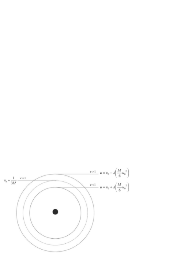
Figure 4.1: Orbit shifts about the classic critical orbit $u_{0}=1/3M$, with corresponding shifts in the speed of light (Not to scale)

.

4.2 Quantum Modified General Geodesics

Using the solutions for the critical circular orbits and the associated impact parameters we can now study how the general photon trajectories are modified due to quantum corrections. In the classic case when a photon comes in from infinity, with the critical impact parameter, it tends to the critical orbit, as was shown in Fig. 2.3; and if we slightly decrease the impact parameter the photon spirals into the singularity, Fig. 2.5. We will now construct a general quantum modified equation of motion and determine how the geodesics change, depending on polarization, as they tend to the critical orbits.

4.2.1 General Vectors

From the quantum modification term in Eqn. (4.1) we can see that in order to construct a general quantum modified geodesic equation we require general photon polarization and wave vectors. The wave vector, $k^{\mu}$, can no longer be represented by a simple constant vector pointing in the $\phi$ direction, as given in the orthonormal frame. And, even though the vertical polarization will remain a constant, as before, the planar polarization will now be a more general vector, constantly changing as the photon moves through the plane.

General Wave Vectors

Our general wave vector will be of the form:

$$k^{\mu}=(\frac{dt}{d\tau},\frac{dr}{d\tau},\frac{d\theta}{d\tau},\frac{d\phi}{d\tau})$$ (4.56)

which respects the light cone condition:

$$0=g_{\mu\nu}k^{\nu}k^{\mu}=F\dot{t}^{2}-F^{-1}\dot{r}^{2}-r^{2}\dot{\phi}^{2}$$ (4.57)

where $g_{\mu\nu}$ is the Schwarzschild metric. Using previous results, of Eqns (2.12) and (2.13), and the fact that we are working in the plane, $\theta=\frac{\pi}{2}$, we can represent three of the wave vector components as:

$$\frac{dt}{d\tau}=EF^{-1}\qquad\frac{d\phi}{d\tau}=\frac{J}{r^{2}}\qquad\frac{d\theta}{d\tau}=0$$ (4.58)

where we have defined:

$$F=(1-\frac{2M}{r})$$ (4.59)

Now using Eqn. (4.57) we can write the final component as:

$$(\frac{dr}{d\tau})^{2} = F^{2}(\frac{dt}{d\tau})^{2}-r^{2}F(\frac{d\phi}{d\tau})^{2}$$

$$\frac{dr}{d\tau} = \sqrt{E^{2}-\frac{J^{2}F}{r^{2}}}=E(1-\frac{D^{2}F}{r^{2}})^{\frac{1}{2}}$$ (4.60)

where we have used $D^{2}=\frac{J^{2}}{E^{2}}$. Now the general wave vector can be written as:

$$k^{\mu}=(EF^{-1},E(1-\frac{D^{2}F}{r^{2}})^{\frac{1}{2}},0,\frac{J}{r^{2}})$$ (4.61)

Also:

$$k_{\mu} = g_{\mu\nu}k^{\nu}$$

$$k_{\mu} = (E,-F^{-1}E(1-\frac{D^{2}F}{r^{2}})^{\frac{1}{2}},0,-J)$$ (4.62)

We now have:

$$k_{\mu}k^{\mu}=E^{2}F^{-1}-F^{-1}E^{2}(1-\frac{D^{2}F}{r^{2}})-\frac{J^{2}}{r^{2}}=0$$

as required. Therefore, eliminating $E$, we have the general wave vectors:

$$k^{\mu} = \frac{J}{D}(F^{-1},(1-\frac{D^{2}F}{r^{2}})^{\frac{1}{2}},0,\frac{D}{r^{2}})$$ (4.63)

$$k_{\mu} = \frac{J}{D}(1,-F^{-1}(1-\frac{D^{2}F}{r^{2}})^{\frac{1}{2}},0,-D)$$ (4.64)

We now need to normalize these vectors so, as they come in from infinity and tend to the critical circular orbit, they correspond to the critical orbit vector (4.8). However, as (4.8) is given in the orthonormal basis, and we are now working in the coordinate frame, we must use the tetrad (A.44), given in Appendix B, to transform (4.8) to its coordinate frame equivalent. Therefore, (4.8) in the coordinate basis is given as:

$$k^{\mu}=(e^{-1})^{\mu}_{a}k^{a}=(e^{-1})^{\mu}_{a}\left(\begin{array}[]{c}E_{k}\\ 0\\ 0\\ E_{k}\\ \end{array}\right)=E_{k}\left(\begin{array}[]{c}F^{-\frac{1}{2}}\\ 0\\ 0\\ \frac{1}{r}\\ \end{array}\right)$$ (4.65)

This now corresponds to a wave vector for a circular orbit in the coordinate frame. To represent the critical orbit we simply substitute for $r=3M$, in which case $F=1-\frac{2M}{r}\rightarrow\frac{1}{3}$, thus (4.65) becomes:

$$k^{\mu}=E_{k}(\sqrt{3},0,0,\frac{1}{3M})$$ (4.66)

Now, if we evaluate (4.64) with $r=3M$ and $D=3\sqrt{3}M$ we have:

$$k^{\mu}=\frac{J}{D}\sqrt{3}(\sqrt{3},0,0,\frac{1}{3M})$$ (4.67)

Therefore, (4.67) is similar to (4.66) up to a constant of normalization, given as:

$$E_{k}=\frac{J}{D}\sqrt{3}=E\sqrt{3}$$ (4.68)

Then, the normalized form of (4.64) is given by using (4.68):

$$k^{\mu}=\frac{E_{k}}{\sqrt{3}}(F^{-1},(1-\frac{D^{2}F}{r^{2}})^{\frac{1}{2}},0,\frac{D}{r^{2}})$$ (4.69)

General Polarization Vectors

Now we need to construct the, planar and vertical, polarization vectors, $a^{\mu}$, of the photon; which must be spacelike normalized as:

$$a_{\mu}a^{\mu}=-1\qquad a_{\mu}k^{\mu}=0$$ (4.70)

As before, as we are working in a plane, the vertical polarization, $a^{\mu}_{1}$, will be a constant, and can simply be written as:

$$a_{1}^{\mu}=(0,0,1,0)$$ (4.71)

To normalize this we do as follows:

$$a_{1\mu}=g_{\mu\nu}a^{\nu}_{1}=-r^{2}(0,0,1,0)\qquad\Rightarrow\qquad a_{1}^{\mu}a_{1\mu}=-r^{2}$$ (4.72)

Therefore, the normalized vertical polarization vector is given as:

$$a_{1}^{\mu} = (0,0,\frac{1}{r},0)$$

$$a_{1\mu} = -r^{2}(0,0,\frac{1}{r},0)$$ (4.73)

These now satisfy both the conditions in (4.70). The planar polarized vector, $a^{\mu}_{2}$, is given in the plane of $r$ and $\phi$:

$$a^{\mu}_{2}=(0,A,0,B)$$ (4.74)

Now, using the two conditions in (4.70) we can determine $A$ and $B$. From:

$$a_{2\mu}=g_{\mu\nu}a_{2}^{\nu}=(0,-AF^{-1},0,-r^{2}B)$$ (4.75)

and the vector (4.69) we have:

$$k^{\mu}a_{2\mu}=(1-\frac{D^{2}F}{r^{2}})^{\frac{1}{2}}(AF^{-1})+(\frac{D}{r^{2}})(r^{2}B)=0$$ (4.76)

$$a^{2\mu}a_{2\mu}=A^{2}F^{-1}+B^{2}r^{2}=-1$$ (4.77)

Solving these for $A$ and $B$:

$$B=-\frac{F^{-1}}{D}(1-\frac{D^{2}F}{r^{2}})^{\frac{1}{2}}A$$ (4.78)

$$A^{2}=\frac{F}{(1+\frac{r^{2}F^{-1}}{D^{2}}(1-\frac{D^{2}F}{r^{2}}))}$$ (4.79)

Therefore, we have:

$$A=\frac{DF}{r}\qquad B=-\frac{1}{r}(1-\frac{D^{2}F}{r^{2}})^{\frac{1}{2}}$$ (4.80)

and the planar polarization vector becomes:

$$a_{2}^{\mu}=(0,\frac{DF}{r},0,-\frac{1}{r}(1-\frac{D^{2}F}{r^{2}})^{\frac{1}{2}})$$ (4.81)

We now have the required polarization vectors:

$$a_{1}^{\mu} = \frac{1}{r}(0,0,1,0)$$ (4.82)

$$a_{1\mu} = -r^{2}(0,0,\frac{1}{r},0)$$ (4.83)

$$a_{2}^{\mu} = \frac{1}{r}(0,DF,0,-(1-\frac{D^{2}F}{r^{2}})^{\frac{1}{2}})$$ (4.84)

$$a_{2\mu} = (0,-\frac{D}{r},0,(1-\frac{D^{2}F}{r^{2}})^{\frac{1}{2}})$$ (4.85)

where subscript 1 and 2 are vertical and planar polarizations respectively. These now satisfy the conditions in (4.70) with the wave vector (4.69).

4.2.2 Quantum Modification

Having derived the general polarization and wave vectors, we can see from Eqn. (3.15) that the quantum modification given by:

$$\delta k(a)=\frac{8c_{\alpha}}{m_{e}^{2}}R_{abcd}k^{a}k^{c}a^{b}a^{d}$$ (4.86)

also requires the Riemann tensor components in the coordinate frame. In Appendix A we have calculated the required components as:

$$R^{\prime}_{trrt} = -\frac{2M}{r^{3}}\qquad R^{\prime}_{\theta rr\theta}=-\frac{MF^{-1}}{r}\qquad R^{\prime}_{\phi rr\phi}=-\frac{MF^{-1}}{r}$$

$$R^{\prime}_{\phi\theta\theta\phi} = 2Mr\qquad R^{\prime}_{\theta t\theta t}=-\frac{MF}{r}\qquad R^{\prime}_{\phi t\phi t}=-\frac{MF}{r}$$ (4.87)

Using this information we will now determine the form of the general quantum modification; and from the polarization rule, this quantum correction should satisfy the condition: $\delta k_{1}^{2}=-\delta k_{2}^{2}$ for the two polarizations.

For vertical $(\theta)$ polarization we have, by using (4.69) and (4.82) in (4.86):

$$R_{abcd}k^{a}k^{c}a_{1}^{b}a_{1}^{d} = R_{a\theta c\theta}\frac{1}{r^{2}}k^{a}k^{c}=R_{t\theta t\theta}\frac{1}{r^{2}}k^{t}k^{t}+R_{r\theta r\theta}\frac{1}{r^{2}}k^{r}k^{r}+R_{\phi\theta\phi\theta}\frac{1}{r^{2}}k^{\phi}k^{\phi}$$ (4.88)

$$= -\frac{MF}{r}(\frac{1}{r^{2}})(\frac{F^{-1}E_{k}}{\sqrt{3}})(\frac{F^{-1}E_{k}}{\sqrt{3}})$$

$$+ \frac{MF^{-1}}{r}(\frac{1}{r^{2}})(\frac{\sqrt{1-\frac{D^{2}F}{r^{2}}}E_{k}}{\sqrt{3}})(\frac{\sqrt{1-\frac{D^{2}F}{r^{2}}}E_{k}}{\sqrt{3}})$$

$$- 2Mr(\frac{1}{r^{2}})(\frac{DE_{k}}{r^{2}\sqrt{3}})(\frac{DE_{k}}{r^{2}\sqrt{3}})$$

$$= -\frac{ME_{k}^{2}F^{-1}}{3r^{3}}+\frac{ME_{k}^{2}F^{-1}(1-\frac{D^{2}F}{r^{2}})}{3r^{3}}-\frac{2ME_{k}^{2}D^{2}}{3r^{5}}$$

$$= -\frac{ME_{k}^{2}D^{2}}{r^{5}}$$

Similarly, for planar ($r-\phi$ plane) polarization we have, by using (4.69) and (4.84) in (4.86):

$$R_{abcd}k^{a}k^{c}a_{2}^{b}a_{2}^{d} = R_{arcr}k^{a}k^{c}a_{2}^{r}a_{2}^{r}+R_{arc\phi}k^{a}k^{c}a_{2}^{r}a_{2}^{\phi}+R_{a\phi cr}k^{a}k^{c}a_{2}^{\phi}a_{2}^{r}$$ (4.89)

$$+ R_{a\phi c\phi}k^{a}k^{c}a_{2}^{\phi}a_{2}^{\phi}$$

$$= R_{trtr}k^{t}k^{t}a_{2}^{r}a_{2}^{r}+R_{\phi r\phi r}k^{\phi}k^{\phi}a_{2}^{r}a_{2}^{r}+R_{\phi rr\phi}k^{\phi}k^{r}a_{2}^{r}a_{2}^{\phi}$$

$$+ R_{r\phi\phi r}k^{r}k^{\phi}a_{2}^{\phi}a_{2}^{r}+R_{t\phi t\phi}k^{t}k^{t}a_{2}^{\phi}a_{2}^{\phi}+R_{r\phi r\phi}k^{r}k^{r}a_{2}^{\phi}a_{2}^{\phi}$$

$$= \frac{2M}{r^{3}}(\frac{F^{-1}E_{k}}{\sqrt{3}})^{2}(\frac{DF}{r})^{2}+\frac{MF^{-1}}{r}(\frac{DE_{k}}{\sqrt{3}r^{2}})^{2}(\frac{DF}{r})^{2}$$

$$+ \frac{MF^{-1}}{r}(\frac{DE_{k}}{\sqrt{3}r^{2}})(\frac{E_{k}}{\sqrt{3}}\sqrt{1-\frac{D^{2}F}{r^{2}}})(\frac{DF}{r})(\frac{\sqrt{1-\frac{D^{2}F}{r^{2}}}}{r})$$

$$+ \frac{MF^{-1}}{r}(\frac{E_{k}\sqrt{1-\frac{D^{2}F}{r^{2}}}}{\sqrt{3}})(\frac{DE_{k}}{\sqrt{3}r^{2}})(\frac{\sqrt{1-\frac{D^{2}F}{r^{2}}}}{r})(\frac{DF}{r})$$

$$- \frac{MF}{r}(\frac{F^{-1}E_{k}}{\sqrt{3}})^{2}(\frac{\sqrt{1-\frac{D^{2}F}{r^{2}}}}{r})^{2}$$

$$+ \frac{MF^{-1}}{r}(\frac{E_{k}\sqrt{1-\frac{D^{2}F}{r^{2}}}}{\sqrt{3}})^{2}(\frac{\sqrt{1-\frac{D^{2}F}{r^{2}}}}{r})^{2}$$

$$= \frac{ME_{k}^{2}D^{2}}{r^{5}}$$

Therefore, the quantum modifications, $k^{2}=\delta k(a)$, for the two polarizations $a_{1}$ and $a_{2}$ (vertical and planar respectively) are:

$$\delta k(a_{1}) = -(\frac{8c_{\alpha}}{m_{e}^{2}})\frac{ME_{k}^{2}D^{2}}{r^{5}}\qquad\textrm{Vertical}$$ (4.90)

$$\delta k(a_{2}) = (\frac{8c_{\alpha}}{m_{e}^{2}})\frac{ME_{k}^{2}D^{2}}{r^{5}}\qquad\textrm{Planar}$$ (4.91)

where $-\delta k(a_{1})=\delta k(a_{2})$, as required. Now, using $k^{\mu}k_{\mu}-\delta k(a)$=0 we can write the general equations of motion for the two polarizations:

$$k^{\mu}k_{\mu}\pm(\frac{8c_{\alpha}}{m_{e}^{2}})\frac{ME_{k}^{2}D^{2}}{r^{5}}=0$$

$$(\frac{dr}{d\tau})^{2}=F^{2}(\frac{dt}{d\tau})^{2}-r^{2}F(\frac{d\phi}{d\tau})^{2}\pm F(\frac{8c_{\alpha}}{m_{e}^{2}})\frac{ME_{k}^{2}D^{2}}{r^{5}}$$

As before, substituting for $\dot{t}$, $\dot{\phi}$ and transforming $r\rightarrow\frac{1}{u}$, we have:

$$(\frac{du}{d\phi})^{2}=\frac{1}{D^{2}}-Fu^{2}\pm(\frac{D^{2}MA}{3})Fu^{5}$$ (4.92)

We can also write $u$ as a function of time:

$$(\frac{du}{dt})^{2}=(Du^{2}F)^{2}(\frac{1}{D^{2}}-Fu^{2}\pm(\frac{D^{2}MA}{3})Fu^{5})$$ (4.93)

where we have used the substitution for $A$ given in equation (4.31). Now, the Eqns. 4.92 and 4.93 are the general equations of motion, $+$ for vertical ($\theta$) polarization and $-$ for planar ($r$-$\phi$) polarization. In these equations we not only use the impact parameter of the form $1/D^{2}$ but also $D^{2}$, therefore the parameters for the two polarizations are given as:

$$\frac{1}{D^{2}}=\frac{u_{0}^{2}}{3}(1\pm AMu_{0})\rightarrow D=\frac{\sqrt{3}}{u_{0}}\mp\frac{\sqrt{3}AM}{2}+\mathcal{O}(A)$$ (4.94)

4.2.3 General Trajectory to the Critical Orbit.

Now that we have the general orbit equation (4.92) we can first test whether, for the critical impact perimeter $D$, the equation $\frac{du}{d\phi}\rightarrow 0$ for first order in $A$. Substituting the critical orbits and the impact parameters given in (4.54),(4.55) and (4.94) into (4.92) and expanding up to first order in $A$ we have: For planar polarization.

$$(\frac{du}{d\phi})^{2} = \frac{u_{0}^{2}}{3}(1+AMu_{0})-[1-2M(u_{0}(1+\frac{AM}{6}u_{0}))[(u_{0}(1+\frac{AM}{6}u_{0})]^{2}$$ (4.95)

$$- (\frac{\frac{3}{u_{0}^{2}(1+AMu_{0})}AM}{3})[1-2M[u_{0}(1+\frac{AM}{6}u_{0})]][u_{0}(1+\frac{AM}{6}u_{0})]^{5}$$

$$\rightarrow 0$$

and similarly for vertical polarization.

$$(\frac{du}{d\phi})^{2} = \frac{u_{0}^{2}}{3}(1-AMu_{0})-[1-2M[u_{0}(1-\frac{AM}{6}u_{0})]][u_{0}(1-\frac{AM}{6}u_{0})]^{2}$$ (4.96)

$$- (\frac{\frac{3}{u_{0}^{2}(1-AMu_{0})}AM}{3})[1-2[(u_{0}(1-\frac{AM}{6}u_{0})]][u_{0}(1-\frac{AM}{6}u_{0})]^{5}$$

$$\rightarrow 0$$

Expanding these and eliminating all terms of order $A^{2}$ and higher, we find that the right hand sides go to zero, as required. Thus for the appropriate impact parameters these equations behave as they should.

The next step is to solve equation (4.92) for the two polarizations. This is most simply done using numerical methods in Mathematica. As a guide, we know our solution will be of the form $u=u_{0}+ku_{1}$, where $u_{0}$ will be the classical solution (2.39), $u_{1}$ will be a small modification that pushes the critical orbit up or down depending on photon polarization, and $k$ will be some constant that is first order in $A$, i.e. of the form $k=As$, where $s$ will be some number given by the boundary condition: for $\phi\rightarrow\infty$ then $u(\phi)\rightarrow u_{0}(1\pm\frac{A}{6}u_{0})$. If we substitute for the critical impact parameter $D$ from (4.54) and (4.55) depending on the polarization, and then transform to $u\rightarrow u_{0}+Asu_{1}$, and expand to first order in $A$, we have non-linear first order differential equations in $u_{0}$, $u_{1}$ and $\phi$.

• For planar polarization:

  $$\frac{du_{1}(\phi)}{d\phi} = \frac{}{6s\sqrt{\frac{1}{27M^{2}}-u_{0}(\phi)^{2}+2Mu_{0}(\phi)^{3}}}[\frac{1}{27M^{2}}-27M^{3}u_{0}(\phi)^{5}$$ (4.97)

  $$+ 54M^{4}u_{0}(\phi)^{6}-6su_{0}(\phi)u_{1}(\phi)+18sMu_{0}(\phi)^{2}u_{1}(\phi)]$$

• For vertical polarization:

  $$\frac{du_{1}(\phi)}{d\phi} = \frac{1}{6s\sqrt{\frac{1}{27M^{2}}-u_{0}(\phi)^{2}+2Mu_{0}(\phi)^{3}}}[-\frac{1}{27M^{2}}+27M^{3}u_{0}(\phi)^{5}$$ (4.98)

  $$- 54M^{4}u_{0}(\phi)^{6}-6su_{0}(\phi)u_{1}(\phi)+18sMu_{0}(\phi)^{2}u_{1}(\phi)]$$

These can be solved in one of two ways, (i) is to substitute the classic solution (2.39) for $u_{0}$ and solve analytically, (ii) is to solve $\frac{du_{1}}{d\phi}$ and the classic equation for $\frac{du_{0}}{d\phi}$ simultaneously using numerical techniques. We attempted to use method (i) to derive an analytic solution for $u_{1}(\phi)$, however, due to the complex nature of the equation we proceeded to use method (ii), that is solving by numerical methods. To do this we set the constant $s=1$, and then when the numerical values of $u_{1}(\phi)$ were determined we could determine the constant $s$ so that $u(\phi)$ coincided with the modified circular orbits given in (4.54) and (4.55). This technique was used for reasons of convenience, because solving (4.97) and (4.98) for various values of $s$ would be time consuming as each numerical calculation takes a significant amount of time; therefore solving them once and then scaling the solution is a more convenient method. The results of the equations were plotted as:

$$u(\phi)=u_{0}(\phi)+Asu_{1}(\phi)$$ (4.99)

where the constant $s$ was picked to satisfy the condition: $\phi\rightarrow\infty$ $\Rightarrow$ $u(\phi)\rightarrow u_{0}(1\pm\frac{A}{6}u_{0})$ i.e. the trajectories tend to the critical orbit, depending on polarization. In this way the constant $s$ was determined to be $s=1/3$, which was tested for various values of $M$. We have plotted the results of the numerical calculation in Figs. 4.2 and 4.3. In Fig. 4.2, you can see that the general critical orbits follow a classic style path, however the orbit splitting is not clearly visible. But in Fig. 4.3 we have plotted a closer view of the critical orbits, and here the splitting is highly visible. It can be seen that the general trajectories for the planar and vertically polarized photons tend to the relevant critical orbits.

Figure 4.2: The quantum modified critical orbits follow classic type paths. We have used a factor $A=0.00009$ in order to make the quantum corrections more visible, where a real value should be of order $\sim 10^{-32}$, Eqn. 4.38. The splitting of the orbits can be clearly seen in the Fig. 4.3, given below.

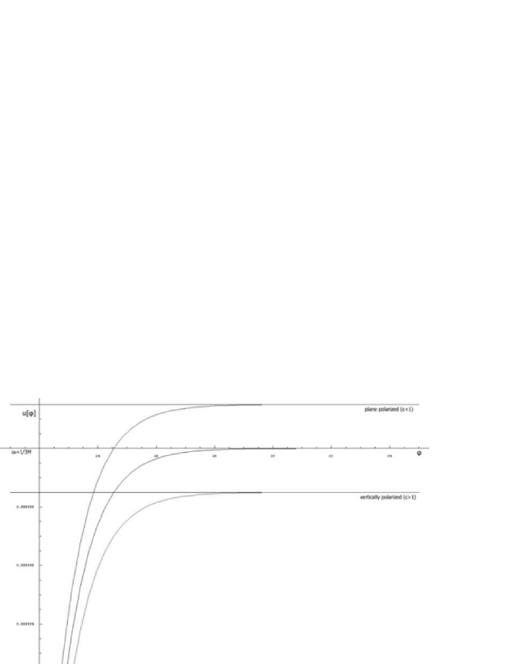
Figure 4.3: The quantum modified trajectories show clear splitting as they tend to the critical points. We used the constants $M=\frac{1}{3}$ and $A=0.00009$.

4.3 Quantum Modification and the Event Horizon

In Chapter. 2 it was shown that when we decreased the impact parameter from the critical value ($D=3\sqrt{3}M$ to $D-1/10$) the photon trajectory, given as $u(\phi)$, spiraled into the singularity, Fig. 2.5; and when we represent the trajectory as a function of coordinate time, $u(t)$, it tends to the event horizon, $u=1/2M$. From the horizon theorem it was seen that quantum modifications have no effect on photon velocities directed normal to the event horizon. So this implies when a photon tends to the event horizon at an angle, e.g. with an impact parameter $D=D_{critical}-1/10$, then the component of velocity normal to the horizon should be unchanged, while the component parallel to it is modified according to the quantum correction; this modification should then result in a shift of the photon trajectory, but the horizon should remain fixed. In order to test this we used Eqn. (4.92) with an impact parameter $D=D_{critical}-1/10$ to show that the photon trajectories still fall into the singularity. We then used Eqn. (4.93), with the new impact parameter, to study the behavior of the trajectories around the event horizon.

4.3.1 Trajectories to the singularity

In order to construct quantum modified trajectories, which go past the critical orbit and fall into the singularity, we require the impact parameters:

$$\frac{1}{D^{2}}=\frac{1}{(\frac{\sqrt{3}}{u_{0}\sqrt{(1\pm AMu_{0})}}-\frac{1}{10})^{2}}\rightarrow D=\frac{\sqrt{3}}{u_{0}}\mp\frac{\sqrt{3}AM}{2}-\frac{1}{10}+\mathcal{O}(A)$$ (4.100)

where, as before, $+$ is for vertical polarization and $-$ is planar polarization, in $1/D^{2}$. For these impact parameters we numerically solved Eqn. (4.92), and in Fig. 4.4 we can see that all the trajectories follow a classic type path into the singularity. However, near the singularity you can see the splitting of the orbits as they tend to $u\rightarrow\infty$. In Fig. 4.5 we have shown a magnified view of the point where the trajectories cross the event horizon. In this figure it can be seen that the planar polarized photon ($c<1$) crosses the event horizon at a point before the classic trajectory and the vertically polarized photon ($c>1$) crosses it at a point after the classic trajectory. This makes sense, as the planar polarized photons are pushed towards the black hole and vertically polarized trajectories are pushed out, the vertically polarized ones must spiral further around the black hole to reach the event horizon compared to the classic or the planar polarized trajectories.

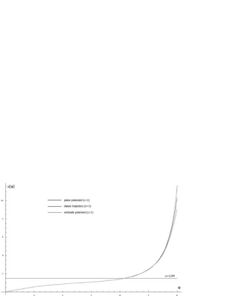
Figure 4.4: The quantum modified trajectories follow similar paths, as the classic trajectory, to the singularity, with $M=\frac{1}{3}$ and $A=0.0009$.

Figure 4.5: The classic and quantum modified trajectories crossing the event horizon $u=2M$, with $M=\frac{1}{3}$ and $A=0.0009$.

4.3.2 Fixed Event Horizon

To demonstrate the fact that the event horizon remains fixed at $u=1/2M$ we applied the impact parameters given by (4.100) to Eqn.(4.93). Again, solving numerically we found that the trajectories tend to the event horizon in the classic way, Fig. 4.6, however, they are again slightly shifted. In Fig. 4.7, a close up of the point where the trajectories tend to the event horizon at $u=1/2M$, you can clearly see that the quantum modified orbits tend to the horizon before the classic orbit. This can be understood by the fact that the planar polarized trajectory is pushed towards the black hole, hence it has less of a distance to propagate before it reaches the horizon, and even though the vertically polarized trajectory is pushed outwards, the fact that it has a faster velocity than $c=1$ it reaches the event horizon before the classic trajectory.

Figure 4.6: The quantum modified trajectories follow similar paths, as the classic trajectory, to the event horizon, with $M=\frac{1}{3}$ and $A=0.0009$.

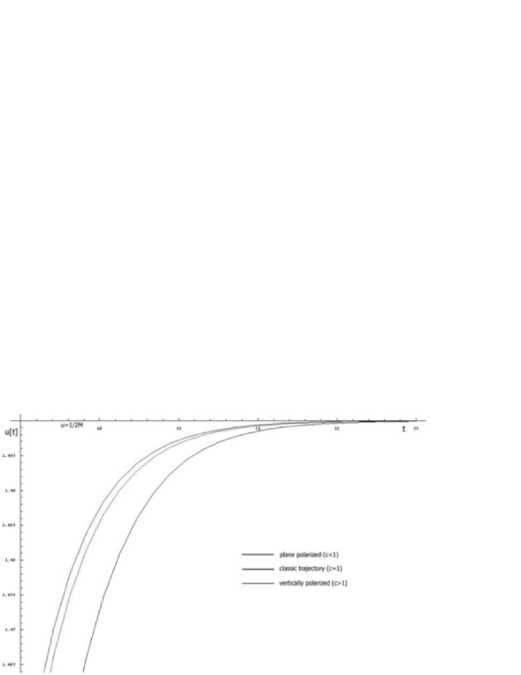
Figure 4.7: The classic and quantum modified trajectories reach the event horizon at differing times, with $M=\frac{1}{3}$ and $A=0.0009$.

The other more important thing we can note from this calculation is that the event horizon remains fixed at the classic point $u=1/2M$, due to the fact that, as was stated earlier, the quantum correction has no effect on photon momentum normal to the horizon. This means even though the quantum correction implies velocities greater than the speed of light, no photons can escape from the event horizon, so the black hole remains black.

Chapter 5 Quantum Modified Schwarzschild Metric

Now, using our previous results, we can construct a new metric that encompasses the quantum corrections due to vacuum polarization. This metric should then be a sum of the classic Schwarzschild metric and the polarization dependent quantum corrections we derived in Eqns. (4.88) and (4.89):

$$\mathcal{G}_{\mu\nu}k^{\mu}k^{\nu} = (g_{\mu\nu}+\mathfrak{g}_{\mu\nu})k^{\mu}k^{\nu}=0$$ (5.1)

$$= (g_{\mu\nu}-\frac{8c_{\alpha}}{m_{e}^{2}}R_{\mu\eta\nu\lambda}a^{\eta}a^{\lambda})k^{\mu}k^{\nu}=0$$

5.1 Construction of the Metric

Using the results in Sec. 4.2.2 we can write the first components of the quantum modified metric $\mathcal{G}_{tt}^{1}$ and $\mathcal{G}_{tt}^{2}$, for vertical and planar polarization respectively, as:

$$\mathcal{G}_{tt}^{1} = g_{tt}-\frac{8c_{\alpha}}{m_{e}^{2}}R_{tbtd}a_{1}^{b}a_{1}^{d}$$ (5.2)

$$= F-\frac{8c_{\alpha}}{m_{e}^{2}}(-\frac{MF}{r})(\frac{1}{r^{2}})$$

$$= F+\frac{AMD^{2}}{9}Fu^{3}$$

$$\mathcal{G}_{tt}^{2} = g_{tt}-\frac{8c_{\alpha}}{m_{e}^{2}}R_{tbtd}a_{2}^{b}a_{2}^{d}$$ (5.3)

$$= F-\frac{8c_{\alpha}}{m_{e}^{2}}[\frac{2M}{r^{3}}(\frac{DF}{r})^{2}-(\frac{MF}{r})(\frac{\sqrt{1-\frac{D^{2}F}{r^{2}}}}{r})^{2}]$$

$$= F-\frac{AMD^{2}}{9}(3D^{2}F^{2}u^{5}-Fu^{3})$$

where, in the last lines of each component, we have used Eqn (4.31) to replace the constants with $A$, and we’ve made the transformation $r\rightarrow 1/u$. Now, doing this for all the other components we can construct the metrics for vertical and planar polarizations:

• Vertical Polarization: $a_{1}^{\mu}=u(0,0,1,0)$

  $$\mathcal{G}^{1}_{\mu\nu}=\left(\begin{array}[]{cccc}F-BFu^{3}&0&0&0\\ 0&-\frac{1}{F}+\frac{Bu^{3}}{F}&0&0\\ 0&0&-\frac{1}{u^{2}}&0\\ 0&0&0&-\frac{1}{u^{2}}-Bu\\ \end{array}\right)$$ (5.4)

• Planar Polarization: $a_{2}^{\mu}=u(0,DF,0,D\frac{du}{d\phi})$

  $$\mathcal{G}^{2}_{\mu\nu}=\left(\begin{array}[]{cccc}F+BFu^{3}(1-3D^{2}Fu^{2})&0&0&0\\ 0&-\frac{1}{F}-\frac{Bu^{3}(1-D^{2}Fu^{2})}{F}&0&Bu^{3}D\frac{du}{d\phi}\\ 0&0&-\frac{1}{u^{2}}&0\\ 0&Bu^{3}D\frac{du}{d\phi}&0&-\frac{1}{u^{2}}-BD^{2}Fu^{3}\\ \end{array}\right)$$ (5.5)

where $B=\frac{AMD^{2}}{9}$. These are now the relevant quantum modified Schwarzschild metrics for vertical and planar polarizations.

5.2 Dynamics with the Quantum Modified Metric

We can now derive the same equations of motion as (4.92), but now we can do it simply with the quantum modified metrics. Using the general wave vector in a plane:

$$k^{\mu} = (\dot{t},\dot{r},\dot{\theta},\dot{\phi})$$ (5.6)

$$= (\frac{J}{D}F^{-1},-J\frac{du}{d\phi},0,Ju^{2})$$

where we have transformed to $r\rightarrow 1/u$, and we substitute for $\dot{t}$ and $\dot{\phi}$ as before. Applying this wave vector to (5.4) and(5.5) we find:

$$0 = \mathcal{G}^{1}_{\mu\nu}k^{\mu}k^{\nu}$$ (5.7)

$$\Rightarrow (\frac{du}{d\phi})^{2}=\frac{1}{D^{2}}-Fu^{2}+(\frac{D^{2}A}{3})Fu^{5}$$

for vertical polarization, and

$$0 = \mathcal{G}^{2}_{\mu\nu}k^{\mu}k^{\nu}$$ (5.8)

$$\Rightarrow (\frac{du}{d\phi})^{2}=\frac{1}{D^{2}}-Fu^{2}-(\frac{D^{2}A}{3})Fu^{5}$$

for planar polarization. These are identical to the equations we derived in Sec. 4.2.2.

Radial Geodesics

We can now show that the metric for vertical polarization is consistent with the fact that radially projected photon trajectories are not modified. By using the vertical polarization metric, (5.4), and a general radial wave vector, ($k^{\mu}=(\dot{t},\dot{r},0,0)$, we find:

$$0 = \mathcal{G}^{1}_{\mu\nu}k^{\mu}k^{\nu}$$

$$\Rightarrow\qquad\frac{dt}{dr} = \pm\frac{1}{F}$$ (5.9)

which is identical to the classic radial geodesic equation, (2.30). However, the same is not true for the planar polarization metric. Due to our derivation of the polarization vectors in Sec. 4.2.1, we constructed a very general vertical polarization vector and then normalized it; however, the one for planar polarization was constructed for the case where $\frac{d\phi}{d\tau}\neq 0$, as can be seen in Eqns. (4.60) and (4.76); therefore the planar polarization vector has $\phi$ dependence "mixed" into it through the substitution of $\dot{\phi}$:

$$(\frac{dr}{d\tau})^{2} = F^{2}(\frac{dt}{d\tau})^{2}-r^{2}F(\frac{d\phi}{d\tau})^{2}$$

$$= (E^{2}-\frac{J^{2}F}{r^{2}})^{\frac{1}{2}}=E(1-\frac{D^{2}F}{r^{2}})^{\frac{1}{2}}$$

We can note that it’s a result of the substitution $\frac{d\phi}{d\tau}=\frac{J}{r^{2}}$, in the polarization vectors, that we acquire an extra parameter $D$ in our quantum correction (apart from the one introduced through normalization, which was incorporated into $B=AD^{2}/9$). We can then say that if we need to use the metric for a radial trajectory with $\frac{d\phi}{d\tau}=0$ we can just set $D=0$, as this would lead to the removal of the $\phi$ dependence. In this way, the planar polarized quantum modified metric for radial trajectories is:

$$\mathcal{G}(\textsl{$\phi$=0})^{2}_{\mu\nu}=\left(\begin{array}[]{cccc}F+BFu^{3}&0&0&0\\ 0&-\frac{1}{F}-\frac{Bu^{3}}{F}&0&0\\ 0&0&-\frac{1}{u^{2}}&0\\ 0&0&0&0\\ \end{array}\right)$$ (5.11)

Then applying this to a general radial wavevector, we again find the classic radial geodesic equation:

$$0 = \mathcal{G}(\textsl{$\phi$=0})^{2}_{\mu\nu}k^{\mu}k^{\nu}$$

$$\Rightarrow\qquad\frac{dt}{dr} = \pm\frac{1}{F}$$ (5.12)

Therefore, we have metrics for the Schwarzschild space time that incorporate quantum corrections due to vacuum polarization; and these metrics are consistent with classic results.

Chapter 6 Summary

For Schwarzschild Spacetime we showed, in the orthonormal frame, that, due to quantum corrections, the stable circular orbit at $u_{0}=1/3M$ splits depending on the polarization of the photon, and the new modified circular orbits are given by the classical orbit plus a correction term to first order in a dimensionless constant $A$: $u=u_{0}+Au_{1}$, where $A=\frac{24c_{\alpha}E_{k}^{2}}{J^{2}m_{e}^{2}}$ and has an order of $10^{-32}$. As stated by the polarization sum rule this splitting of the critical orbit is equal in magnitude but opposite in sign for the two polarizations. We found that the vertically polarized photon (c>1) is pushed out by a correction of $u_{1}=-\frac{M}{6}u_{0}^{2}$, while the planar polarized photon is pulled in by a correction of $u_{1}=\frac{M}{6}u_{0}^{2}$. It was also found that this orbit shift also requires an appropriate modification of the classic impact parameter $\frac{1}{D_{0}^{2}}=\frac{u_{0}^{2}}{3}$. This modification, for the quantum corrected orbits, took the form $\frac{1}{D^{2}}=\frac{1}{D_{0}^{2}}+AD_{1}$, and again as for the orbit shift, the change was equal in magnitude but opposite in sign for the two polarizations: $D_{1}=\frac{Mu_{0}^{3}}{3}$ for planar polarization and $D_{1}=-\frac{Mu_{0}^{3}}{3}$ for vertical polarization. Using this information, for the splitting of circular orbits, we then constructed the quantum corrected general equations of motion for the Schwarzschild spacetime. Using these equation of motion it was shown that a photon starting at $u=0$, with the appropriate critical impact parameter, tends to the critical orbit associated with that impact parameter - and the trajectory follows a similar path to the classic case.

We then went on to show that, using the general quantum corrected equations of motion, a photon projected towards the black hole with an impact parameter less than the critical value falls into the the singularity, in terms of the angular distance ($\phi$). Although the photons follow a classic type path into the singularity, the trajectories are slightly shifted according to polarization. The planar polarized photon crosses the horizon before the classic trajectory, and the vertically polarized one crosses it after, this corresponds to the fact that planar polarized photons are pulled towards the black hole and vertically polarized ones are pushed away, hence the vertically polarized ones need to go a further angular distance to reach the event horizon.

In terms of coordinate time ($t$) we found that the photon trajectories tend to the event horizon. Therefore, the quantum corrections do not shift the classic event horizon from $u=\frac{1}{2M}$, which corresponds to the horizon theorem. Also, we found that, although the quantum corrected orbits follow a classic type path to the event horizon, the point at which they hit the horizon is, again, slightly shifted depending on polarization. However, this time both polarizations hit the horizon before the classic trajectory. The planar polarized photon tends to arrive at the horizon first, then the vertically polarized one, and finally the classic photon. This could correspond to the fact that the planar polarized photon, although it has a velocity lower than the speed of light, has less of a distance to go, as its trajectory is pulled towards the black hole. For the vertically polarized case, even though it has a faster than light velocity, it has a further distance to go to reach the horizon as its trajectory is pushed away from the black hole.

Having determined the equations of motion, with the quantum correction, we then went on to construct a Schwarzschild metric that incorporates the quantum correction: $\mathcal{G}_{\mu\nu}=(g_{\mu\nu}+\mathfrak{g}_{\mu\nu})$, where the correction: $\mathfrak{g}_{\mu\nu}$ was again first order in $A$. We showed that with this metric and a general photon wave vector, $k^{\mu}$, we obtain the quantum modified equations of motion, as before. Also, this new metric confirms the horizon theorem, that is, when we use a wave vector indicating a radially projected photon we obtain the classic equation of motions. This was fine for vertical polarization, however, in the planar polarization case we had a problem; we had previously used a substitution that mixed a "hidden" radial angle, $\phi$, into our polarization vector (as in general orbits the planar polarization depends on $\phi$). By tracing back to the origin of this substitution we found that, in order to study radial trajectories, we need to set $D=0$, this then removes the $\phi$ dependency; this then gives us the classic equation of motion for planar polarized radially projected photons.

So in conclusion, after studying the dynamics of null trajectories in Schwarzschild spacetime we derived the polarization dependent photon trajectories to first order in the constant $A$ (which is dependent on the fine structure constant, the mass of the star, mass of the electron, and the energy of the photon). We then incorporated these modification into a general quantum modified metric, which could also be used to derive the general quantum modified equations of motion. Also, the results of this work coincide with the conditions of the horizon theorem and the polarization sum rule.

Appendix A Schwarzschild Spacetime

The ’Schwarzschild geometry’ describes a spherically symmetric spacetime outside a star, and its properties are determined by one parameter, the mass M. The Schwarzschild metric, in spherical polar coordinates, takes the form:

$$g_{\mu\nu}=\left(\begin{array}[]{cccc}F&0&0&0\\ 0&-F^{-1}&0&0\\ 0&0&-r^{2}&0\\ 0&0&0&-r^{2}\sin(\theta)\\ \end{array}\right)$$ (A.1)

This type of spacetime geometry is said to be static, due to the fact that (i) all metric components are independent of $t$, and (ii) the geometry is unchanged by time reversal, $t\rightarrow-t$.

A.1 Geodesic Equations

The equations of motion in Schwarzschild spacetime can be derived by using the covariant form of Newton’s second law of motion,

$$F^{\mu} = \frac{Dp^{\mu}}{D\tau}$$ (A.2)

$$= \frac{dp^{\mu}}{d\tau}+\Gamma^{\mu}_{\nu\rho}\frac{dx^{\nu}}{d\tau}p^{\rho}$$

where we have $p^{\mu}=m\frac{dx^{\mu}}{d\tau}$, and for free fall we have $F^{\mu}=0$, then the equations of motion are:

$$0=\frac{d^{2}x^{\mu}}{d\tau^{2}}+\Gamma^{\mu}_{\nu\rho}\frac{dx^{\nu}}{d\tau}\frac{dx^{\rho}}{d\tau}$$ (A.3)

Now, using this and the appropriate Christoffels we are able to determine the equations of motion. Alternatively, by using the Schwarzschild Lagrangian

$$L=\frac{1}{2}[(1-\frac{2M}{r})\dot{dt}^{2}-(1-\frac{2M}{r})^{-1}\dot{dr}^{2}-r^{2}\dot{d\theta}^{2}-(r^{2}\sin^{2}\theta)\dot{d\phi}^{2}]$$ (A.4)

we find

$$\frac{\partial L}{\partial t} = 0\qquad\frac{\partial L}{\partial\dot{t}}=(1-\frac{2M}{r})\dot{t}$$

$$\frac{d}{d\lambda}\frac{\partial L}{\partial\dot{t}} = (1-\frac{2M}{r})\ddot{t}+\frac{2M}{r^{2}}\dot{r}\dot{t}$$

$$\frac{\partial L}{\partial r} = \frac{M}{r^{2}}\dot{t}^{2}+\frac{M}{r}^{2}(1-\frac{2M}{r})^{-2}\dot{r}^{2}-r\dot{\theta}^{2}-r\dot{\phi}^{2}\sin^{2}\theta$$

$$\frac{\partial L}{\partial\dot{r}} = -(1-\frac{2M}{r})^{-1}\dot{r}$$

$$\frac{d}{d\lambda}\frac{\partial L}{\partial\dot{r}} = -(1-\frac{2M}{r})^{-1}\ddot{r}+\frac{2M}{r^{2}}(1-\frac{2M}{r})^{-2}\dot{r}\dot{r}$$

$$\frac{\partial L}{\partial\theta} = -r^{2}\sin\theta\cos\theta\dot{\phi}^{2}\qquad\frac{\partial L}{\partial\dot{\theta}}=-r^{2}\dot{\theta}$$

$$\frac{d}{d\lambda}\frac{\partial L}{\partial\dot{\theta}} = -2r\dot{r}\dot{\theta}-r^{2}\ddot{\theta}$$

$$\frac{\partial L}{\partial\phi} = 0\qquad\frac{\partial L}{\partial\dot{\phi}}=-r^{2}\sin^{2}\theta\dot{\phi}^{2}$$

$$\frac{d}{d\lambda}\frac{\partial L}{\partial\dot{\phi}} = -2r\dot{r}\sin^{2}\theta\dot{\phi}-2r^{2}\sin\theta\cos\theta\dot{\phi}-r^{2}\sin^{2}\theta\ddot{\phi}$$

and substituting into the Euler equation

$$\frac{\partial L}{\partial x^{\mu}}-\frac{d}{d\lambda}\frac{\partial L}{\partial\dot{x}^{\mu}}=0$$ (A.9)

we have the equations of motion for Schwarzschild spacetime

$$0 = (1-\frac{2M}{r})\ddot{t}+\frac{2M}{r^{2}}\dot{r}\dot{t}=0$$ (A.10)

$$0 = \frac{M}{r^{2}}\dot{t}^{2}-r\dot{\theta}^{2}-r\dot{\phi}^{2}\sin^{2}\theta+(1-\frac{2M}{r})^{-1}\ddot{r}$$ (A.11)

$$- \frac{M}{r^{2}}(1-\frac{2M}{r})^{-2}\dot{r}^{2}$$

$$0 = -r^{2}\sin\theta\cos\theta\dot{\phi}^{2}+2r\dot{r}\dot{\theta}+r^{2}\ddot{\theta}$$ (A.12)

$$0 = 2r\dot{r}\sin^{2}\theta\dot{\phi}+2r^{2}\sin\theta\cos\theta\dot{\phi}+r^{2}\sin^{2}\theta\ddot{\phi}$$ (A.13)

A.2 Riemann Components in the Orthonormal Frame

The spacetime line interval, Eqn. (1.11), can be rewritten using tetrad transformations (discussed in the next section):

$$\omega^{t}=(1-\frac{2M}{r})^{\frac{1}{2}}dt\qquad\omega^{r}=(1-\frac{2M}{r})^{-\frac{1}{2}}dr\qquad\omega^{\theta}=rd\theta\qquad\omega^{\phi}=r\sin(\theta)d\phi$$ (A.14)

as

$$ds^{2}=(\omega^{t})^{2}-(\omega^{r})^{2}-(\omega^{\theta})^{2}-(\omega^{\phi})^{2}$$ (A.15)

This now has the Minkowski metric

$$g_{\mu\nu}=\left(\begin{array}[]{cccc}1&0&0&0\\ 0&-1&0&0\\ 0&0&-1&0\\ 0&0&0&-1\\ \end{array}\right)$$ (A.16)

Noting that the metric can be written as:

$$dg_{\mu\nu}=\omega_{\mu\nu}+\omega_{\nu\mu}$$ (A.17)

and using the fact that:

$$dg_{\mu\nu}=\frac{\partial g_{\mu\nu}}{\partial x^{\alpha}}dx^{\alpha}=0$$ (A.18)

we then have[2]:

$$\omega_{\mu\nu}=-\omega_{\nu\mu}$$ (A.19)

which implies $\omega$ is antisymmetric, i.e. it has only six unique components and $\omega_{\mu\nu}=0$ for $\mu=\nu$; and we have the conditions:

$$\omega^{0}_{i}=\omega^{i}_{0}\qquad\omega^{i}_{j}=-\omega^{j}_{i}$$ (A.20)

We can now write the exterior derivatives of $\omega^{\mu}$

$$d\omega^{t} = \frac{1}{2}(1-\frac{2M}{r})^{-\frac{1}{2}}(\frac{2M}{r^{2}})dr\wedge dt$$ (A.21)

$$= \frac{M}{r^{2}}(1-\frac{2M}{r})^{-\frac{1}{2}}\omega^{r}\wedge\omega^{t}$$

$$d\omega^{r} = 0$$ (A.22)

$$d\omega^{\theta} = dr\wedge d\theta=\frac{1}{r}(1-\frac{2M}{r})^{\frac{1}{2}}\omega^{r}\wedge\omega^{\theta}$$ (A.23)

$$d\omega^{\phi} = \sin(\theta)dr\wedge d\phi+r\cos(\phi)d\theta\wedge d\phi$$ (A.24)

$$= \frac{1}{r}(1-\frac{2M}{r})^{\frac{1}{2}}\omega^{r}\wedge\omega^{\phi}+\frac{\cot(\theta)}{r}\omega^{\theta}\wedge\omega^{\phi}$$

Now, using Cartan’s equation

$$d\omega^{\mu}=\omega^{\alpha}\wedge\omega^{\mu}_{\alpha}+\Omega^{\mu}$$ (A.25)

with zero torsion $(\Omega^{\mu}=0)$, we can write

$$d\omega^{t} = \omega^{r}\wedge\omega^{t}_{r}+\omega^{\theta}\wedge\omega^{t}_{\theta}+\omega^{\phi}\wedge\omega^{t}_{\phi}$$ (A.26)

$$d\omega^{r} = \omega^{t}\wedge\omega^{r}_{t}+\omega^{\theta}\wedge\omega^{r}_{\theta}+\omega^{\phi}\wedge\omega^{r}_{\phi}$$ (A.27)

$$d\omega^{\theta} = \omega^{t}\wedge\omega^{\theta}_{t}+\omega^{r}\wedge\omega^{\theta}_{r}+\omega^{\phi}\wedge\omega^{\theta}_{\phi}$$ (A.28)

$$d\omega^{\phi} = \omega^{t}\wedge\omega^{\phi}_{t}+\omega^{r}\wedge\omega^{\phi}_{r}+\omega^{\theta}\wedge\omega^{\phi}_{\theta}$$ (A.29)

Comparing Eqns. (A.21)-(A.24) with Eqns. (A.26)-(A.29) we find the six unique components of $\omega^{\mu}_{\nu}$ as

$$\omega^{t}_{r} = \frac{M}{r^{2}}(1-\frac{2M}{r})^{-\frac{1}{2}}\omega^{t}=\frac{M}{r^{2}}dt=\omega^{r}_{t}$$ (A.30)

$$\omega^{\theta}_{r} = \frac{1}{r}(1-\frac{2M}{r})^{\frac{1}{2}}\omega^{\theta}=(1-\frac{2M}{r})^{\frac{1}{2}}d\theta=-\omega^{r}_{\theta}$$ (A.31)

$$\omega^{\phi}_{r} = \frac{1}{r}(1-\frac{2M}{r})^{\frac{1}{2}}\omega^{\phi}=\sin(\theta)(1-\frac{2M}{r})^{\frac{1}{2}}d\phi=-\omega^{r}_{\phi}$$ (A.32)

$$\omega^{\phi}_{\theta} = \frac{\cot(\theta)}{r}\omega^{\phi}=\cos(\theta)d\phi=-\omega^{\theta}_{\phi}$$ (A.33)

$$\omega^{\theta}_{t} = \omega^{t}_{\theta}=0$$ (A.34)

$$\omega^{\phi}_{t} = \omega^{t}_{\phi}=0$$ (A.35)

Now, using:

$$R^{\mu}_{\nu}=d\omega^{\mu}_{\nu}+\omega^{\mu}_{\alpha}\wedge\omega^{\alpha}_{\nu}$$ (A.36)

we can write the six independent components of the Riemann tensor:

$$R^{t}_{r} = d\omega^{t}_{r}+\omega^{t}_{\alpha}\wedge\omega^{\alpha}_{r}=d\omega^{t}_{r}+\omega^{t}_{\theta}\wedge\omega^{\theta}_{r}+\omega^{t}_{\phi}\wedge\omega^{\phi}_{r}$$

$$= -\frac{2M}{r^{3}}dr\wedge dt=-\frac{2M}{r^{3}}\omega^{r}\wedge\omega^{t}$$

$$\Rightarrow R^{t}_{rrt}=R_{trrt}=-\frac{2M}{r^{3}}$$

$$R^{\theta}_{r} = d\omega^{\theta}_{r}+\omega^{\theta}_{\alpha}\wedge\omega^{\alpha}_{r}=d\omega^{\theta}_{r}+\omega^{\theta}_{t}\wedge\omega^{t}_{r}+\omega^{\theta}_{\phi}\wedge\omega^{\phi}_{r}$$

$$= \frac{1}{2}(1-\frac{2M}{r})^{-\frac{1}{2}}\frac{2M}{r^{2}}dr\wedge d\theta=\frac{M}{r^{3}}\omega^{r}\wedge\omega^{\theta}$$

$$\Rightarrow R^{\theta}_{rr\theta}=-R_{\theta rr\theta}=\frac{M}{r^{3}}$$

$$R^{\phi}_{r} = d\omega^{\phi}_{r}+\omega^{\phi}_{\alpha}\wedge\omega^{\alpha}_{r}=d\omega^{\phi}_{r}+\omega^{\phi}_{t}\wedge\omega^{t}_{r}+\omega^{\phi}_{\theta}\wedge\omega^{\theta}_{r}$$

$$= \cos(\theta)(1-\frac{2M}{r})^{\frac{1}{2}}d\theta\wedge d\phi+\sin(\theta)\frac{M}{r^{2}}(1-\frac{2M}{r})^{-\frac{1}{2}}dr\wedge d\phi$$

$$+ \cos(\theta)(1-\frac{2M}{r})^{1}{2}d\phi\wedge d\theta$$

$$= \frac{\cot(\theta)}{r^{2}}(1-\frac{2M}{r})^{\frac{1}{2}}\omega^{\theta}\wedge\omega^{\phi}+\frac{M}{r^{3}}\omega^{r}\wedge\omega^{\phi}$$

$$+ \frac{\cot(\theta)}{r^{2}}(1-\frac{2M}{r})^{\frac{1}{2}}\omega^{\phi}\wedge\omega^{\theta}=\frac{M}{r^{3}}\omega^{r}\wedge\omega^{\phi}$$

$$\Rightarrow R^{\phi}_{rr\phi}=-R_{\phi rr\phi}=\frac{M}{r^{3}}$$

$$R^{\phi}_{\theta} = d\omega^{\phi}_{\theta}+\omega^{\phi}_{\alpha}\wedge\omega^{\alpha}_{\theta}=d\omega^{\phi}_{\theta}+\omega^{\phi}_{t}\wedge\omega^{t}_{\theta}+\omega^{\phi}_{r}\wedge\omega^{r}_{\theta}$$

$$= -\sin(\theta)d\theta\wedge d\phi-\sin(\theta)(1-\frac{2M}{r})d\phi\wedge d\theta$$

$$= -\frac{1}{r^{2}}\omega^{\theta}\wedge\omega^{\phi}+\frac{1}{r^{2}}(1-\frac{2M}{r})\omega^{\theta}\wedge\omega^{\phi}=-\frac{2M}{r^{3}}\omega^{\theta}\wedge\omega^{\phi}$$

$$\Rightarrow R^{\phi}_{\theta\theta\phi}=-R_{\phi\theta\theta\phi}=-\frac{2M}{r^{3}}$$

$$R^{\theta}_{t} = d\omega^{\theta}_{t}+\omega^{\theta}_{\alpha}\wedge\omega^{\alpha}_{t}=d\omega^{\theta}_{t}+\omega^{\theta}_{r}\wedge\omega^{r}_{t}+\omega^{\theta}_{\phi}\wedge\omega^{\phi}_{t}$$

$$= \frac{M}{r^{2}}(1-\frac{2M}{r})^{\frac{1}{2}}d\theta\wedge dt=\frac{M}{r^{3}}\omega^{\theta}\wedge\omega^{t}$$

$$\Rightarrow R^{\theta}_{t\theta t}=-R_{\theta t\theta t}=\frac{M}{r^{3}}$$

$$R^{\phi}_{t} = d\omega^{\phi}_{t}+\omega^{\phi}_{\alpha}\wedge\omega^{\alpha}_{t}=d\omega^{\phi}_{t}+\omega^{\phi}_{r}\wedge\omega^{r}_{t}+\omega^{\phi}_{\theta}\wedge\omega^{\theta}_{t}$$

$$= \frac{M}{r^{2}}(1-\frac{2M}{r})^{\frac{1}{2}}\sin(\theta)d\theta\wedge dt=\frac{M}{r^{3}}\omega^{\phi}\wedge\omega^{t}$$

$$\Rightarrow R^{\phi}_{t\phi t}=-R_{\phi t\phi t}=\frac{M}{r^{3}}$$

A.3 Tetrad Transformation

In Eqn. (A.14) we transformed from the coordinate frame to an orthonormal frame. This is achieved by using the tetrad of the form:

$$e^{a}_{\mu}=\left(\begin{array}[]{cccc}F^{\frac{1}{2}}&0&0&0\\ 0&F^{-\frac{1}{2}}&0&0\\ 0&0&r&0\\ 0&0&0&r\sin(\theta)\\ \end{array}\right)$$ (A.43)

This takes a 4-vector, given in the coordinate frame, and maps it to the equivalent in the orthonormal frame. We can then determine the inverse tetrad, i.e. a tetrad that takes vectors in the orthonormal frame and maps them to the coordinate frame. We find this by using the inverse of (A.43),

$$(e^{-1})^{\mu}_{a}=\left(\begin{array}[]{cccc}F^{-\frac{1}{2}}&0&0&0\\ 0&F^{\frac{1}{2}}&0&0\\ 0&0&\frac{1}{r}&0\\ 0&0&0&\frac{1}{r\sin(\theta)}\\ \end{array}\right),$$ (A.44)

which has the property:

$$e^{a}_{\mu}(e^{-1})^{\mu}_{b}=\delta^{a}_{b}$$ (A.45)

Therefore, (A.44) takes vectors in the orthonormal frame and maps them to the coordinate frame.

A.4 Riemann Components in the Coordinate Frame

In Sec. A.2 the unique components of the Riemann tensor were calculated in the orthonormal frame. In order to determine the components in the coordinate basis we will use the transformation tetrad given in Eqn. A.44. Before we can us the tetrad, (A.44), we need to adjust it so it is able to take covectors in the orthonormal frame, rather than vectors:

$$(e^{-1})^{\mu}_{a}g_{\mu\nu}\eta^{ab}=(e^{-1})_{\nu}^{b}=\left(\begin{array}[]{cccc}F^{\frac{1}{2}}&0&0&0\\ 0&F^{-\frac{1}{2}}&0&0\\ 0&0&r&0\\ 0&0&0&r\\ \end{array}\right),$$ (A.46)

which is just Eqn. (A.43). Then using this we have:

$$\Rightarrow\qquad A_{\mu}(\textrm{coordinate frame})=(e^{-1})_{\mu}^{a}A_{a}(\textrm{orthonormal frame})$$

Now using this tetrad we can transform the orthonormal Riemann tensor components as:

$$R_{\mu\nu\alpha\beta}=(e^{-1})_{\mu}^{a}(e^{-1})_{\nu}^{b}(e^{-1})_{\alpha}^{c}(e^{-1})_{\beta}^{d}R_{abcd}$$

Now using the components given in Sec. A.2 we have:

$$R^{\prime}_{trrt} = (e^{-1})_{t}^{t}(e^{-1})_{r}^{r}(e^{-1})_{r}^{r}(e^{-1})_{t}^{t}R_{trrt}=F^{\frac{1}{2}}F^{-\frac{1}{2}}F^{-\frac{1}{2}}F^{\frac{1}{2}}(-\frac{2M}{r^{3}})=-\frac{2M}{r^{3}}$$

$$R^{\prime}_{\theta rr\theta} = (e^{-1})_{\theta}^{\theta}(e^{-1})_{r}^{r}(e^{-1})_{r}^{r}(e^{-1})_{\theta}^{\theta}R_{\theta rr\theta}=rF^{-\frac{1}{2}}F^{-\frac{1}{2}}r(-\frac{M}{r^{3}})=-\frac{MF^{-1}}{r}$$

$$R^{\prime}_{\phi rr\phi} = (e^{-1})_{\phi}^{\phi}(e^{-1})_{r}^{r}(e^{-1})_{r}^{r}(e^{-1})_{\phi}^{\phi}R_{\phi rr\phi}=rF^{-\frac{1}{2}}F^{-\frac{1}{2}}r(-\frac{M}{r^{3}})=-\frac{MF^{-1}}{r}$$

$$R^{\prime}_{\phi\theta\theta\phi} = (e^{-1})_{\phi}^{\phi}(e^{-1})_{\theta}^{\theta}(e^{-1})_{\theta}^{\theta}(e^{-1})_{\phi}^{\phi}R_{\phi\theta\theta\phi}=rrrr(\frac{2M}{r^{3}})=2Mr$$

$$R^{\prime}_{\theta t\theta t} = (e^{-1})_{\theta}^{\theta}(e^{-1})_{t}^{t}(e^{-1})_{\theta}^{\theta}(e^{-1})_{t}^{t}R_{\theta t\theta t}=rF^{\frac{1}{2}}rF^{\frac{1}{2}}(-\frac{M}{r^{3}})=-\frac{MF}{r}$$

$$R^{\prime}_{\phi t\phi t} = (e^{-1})_{\phi}^{\phi}(e^{-1})_{t}^{t}(e^{-1})_{\phi}^{\phi}(e^{-1})_{t}^{t}R_{\phi t\phi}t=rF^{\frac{1}{2}}rF^{\frac{1}{2}}(-\frac{M}{r^{3}})=-\frac{MF}{r}$$

Therefore, the Riemann tensor components in the coordinate frame are given as:

$$R^{\prime}_{trrt} = -\frac{2M}{r^{3}}\qquad R^{\prime}_{\theta rr\theta}=-\frac{MF^{-1}}{r}\qquad R^{\prime}_{\phi rr\phi}=-\frac{MF^{-1}}{r}$$

$$R^{\prime}_{\phi\theta\theta\phi} = 2Mr\qquad R^{\prime}_{\theta t\theta t}=-\frac{MF}{r}\qquad R^{\prime}_{\phi t\phi t}=-\frac{MF}{r}$$

Bibliography

- [1] I.T. Drummond and S. Hathrell, Phys. Rev. D22 (1980) 343.
- [2] S. Chandrasekhar, The Mathematical Theory of Black Holes, Oxford Science Publications.
- [3] S. Weinberg, Gravitation and Cosmology, Wiley.
- [4] I. R. Kenyon, General Relativity, Oxford.
- [5] G. M. Shore, Quantum Gravitational Optics, (2003) gr-qc/0304059.
- [6] P. Schneider J. Ehlers E. E. Falco, Gravitationl Lenses, Springer-Verlag.
- [7] G. M. Shore, "Faster Than Light" Photons in Gravitational Fields - Causality, Anomalies and Horizons, (1995) gr-qc/9504041.
- [8] R. D. Daniels G. M. Shore, Faster Than Light Photons and Rotating Black Holes, (1995) gr-qc/9508048.
- [9] S. W. Hawking G. F. R. Ellis, The Large Scale Structure of Spacetime, (1973) Cambridge University Press.
- [10] G. M. Shore, Causality and Superluminal Light, (2003) gr-qc/0302116.