Towards the graviton from spinfoams:
higher order corrections in the 3d toy model

Abstract

We consider the recent calculation RovelliProp of the graviton propagator in the spinfoam formalism. Within the 3d toy model introduced in Io , we test how the spinfoam formalism can be used to construct the perturbative expansion of graviton amplitudes. Although the 3d graviton is a pure gauge, one can choose to work in a gauge where it is not zero and thus reproduce the structure of the 4d perturbative calculations. We compute explicitly the next to leading and next to next to leading orders, corresponding to one–loop and two–loop corrections. We show that while the first arises entirely from the expansion of the Regge action around the flat background, the latter receives contributions from the microscopic, non Regge–like, quantum geometry. Surprisingly, this new contribution reduces the magnitude of the next to next to leading order. It thus appears that the spinfoam formalism is likely to substantially modify the conventional perturbative expansion at higher orders.

This result supports the interest in this approach. We then address a number of open issues in the rest of the paper. First, we discuss the boundary state ansatz, which is a key ingredient in the whole construction. We propose a way to enhance the ansatz in order to make the edge lengths and dihedral angles conjugate variables in a mathematically well–defined way. Second, we show that the leading order is stable against different choices of the face weights of the spinfoam model; the next to leading order, on the other hand, is changed in a simple way, and we show that the topological face weight minimizes it. Finally, we extend the leading order result to the case of a regular, but not equilateral, tetrahedron.

I Introduction

The spinfoam formalism carlo is a candidate covariant approach to a non–perturbative quantisation of General Relativity (GR). At present, it provides a consistent background independent theory at the Planck scale, where it describes spacetime as a discrete quantum geometry. However, the large scale behaviour of the theory is less understood. Indeed, the formalism lacks a well–defined procedure to study the semiclassical limit, to define particle scattering amplitudes and to reproduce low–energy physics. In particular, considering the pure gravity case, we would expect to recover in the low–energy regime the conventional perturbative expansion described in term of gravitons. Recently, an important step towards this semiclassical limit has been taken with a proposal for the construction of the 2-point function of quantum gravity from the spinfoam amplitudes ModestoProp . It relies on the use of the propagation kernel (see for instance Mattei ) and on a boundary state peaked around flat geometry. The proposal has been considered in 4d RovelliProp ; noi and 3d Io Riemannian GR without matter. In both cases the large scale limit of the linearised 2-point function has been shown to reproduce the expected $1/p^{2}$ behaviour of the free graviton, thus providing a first piece of evidence that spinfoams might correctly lead back to general relativity in the semiclassical limit.

One of the appealing aspects of the proposal is that it can be used to compute not only the free propagator, but also the quantum corrections due to the intrinsic non–linearity of the theory. Such corrections have been studied in the conventional (non–renormalisable) perturbative approach to quantum gravity, where they are understood as graviton self–energies. In the (physically interesting) 4d case, these give rise to corrections to the Newton potential (see for instance Donoghue ; bohr ). However, the perturbative approach can only be considered as an effective field theory, and not as a complete theory, precisely because of its non–renormalisability: an infinite counterterm arises at two loops Goroff . On the other hand, it has been argued that the cure to this non–renormalisabily could lie in the use of non–perturbative approaches, such as the spinfoam formalism. It is thus very interesting to compute the quantum corrections to the free propagator within the spinfoam formalism, both to give stronger support to the proposal of ModestoProp , and to understand how full quantum gravity modifies the usual perturbative expansion of gravitons.

As a warm up exercise for the 4d case, we consider in this paper 3d quantum gravity and study the emergence of higher order corrections to the free propagator. As is well known, 3d general relativity (GR) has no local degrees of freedom. Due to this peculiarity of the 3d case, the following clarification is necessary. If the metric is quantised as a whole, the theory is exactly solvable Ponzano ; Witten , and this is the basis of the topological Ponzano–Regge (PR) model that we consider here. However, if one treats the metric with the conventional perturbative expansion $g_{\mu\nu}=\eta_{\mu\nu}+h_{\mu\nu}$, the field $h_{\mu\nu}$ is a pure gauge quantity: consequently, the quantum theory does not have a propagating graviton Deser . It is nonetheless useful to consider the above expansion in a gauge where $h_{\mu\nu}$ is not zero. Then the 2-point function,

$$W_{\mu\nu\rho\sigma}(x,y)=\langle{0}|\,{\rm T}\left\{h_{\mu\nu}(x)h_{\rho\sigma}(y)\right\}|{0}\rangle,$$

can be evaluated in a perturbative expansion in $\ell_{\rm P}$. The leading order, corresponding to the free theory, goes as $1/p^{2}$ in momentum space, which in 3d means a $1/\ell$ dependence on the spacetime distance; analogously one can compute the self–energies, and the perturbative expansion is not renormalisable Deser ; Anselmi , as in 4d. Therefore, it makes sense to study in 3d how the spinfoam–defined 2-point function can cure the non–renormalisability of GR by producing a different perturbative expansion than the usual one.

To that end, we consider here a simple toy model introduced in Io : the contribution to the graviton propagator by a single tetrahedron belonging to a discretisation of spacetime. A key advantage of this toy model is that it allows efficient numerical simulations, which are substantially more difficult in the 4d case. Indeed, it was the first numeric results of Io that gave hints of deviations at short scales from the inverse power law $1/\ell$. There is a precise reason to expect that such corrections would show a different structure than the conventional perturbative expansion, and that is the modification of microscopic structure by quantum geometry. To see why this can be expected, recall first that since we are dealing with 3d Riemannian GR, we consider the Ponzano–Regge spinfoam model. It is constructed in terms of half–integers (spins) labelling $\mathrm{SU}(2)$ irreducible representations (irreps), variables which are related to geometric quantities. The large scale limit then corresponds to the large spin limit. In that regime, the model is dominated by the path integral for Regge calculus, with a specific choice of measure. Regge calculus is a discrete approximation to classical GR, which captures the non–linearity of the theory. Therefore, in this limit, one can still expand around a flat background, and consider only small perturbations around it. The leading order, which reproduces the $1/\ell$ free graviton, is obtained by keeping only the quadratic term in the Regge action, and the trivial background measure. Higher orders in the action and in the measure give corrections with the structure of the usual continuum perturbative expansion.

Thus far, one would conclude that the spinfoam formalism simply produces a somewhat discrete version of the conventional theory. However, because the Regge path integral only emerges in the large spin limit, the full theory predicts further sources of corrections, arising from the exact, non Regge–like, quantum geometry. Heuristically, these corrections are remnants at large scales of the discrete microscopic structure of the spinfoam geometry. These other corrections have no analogue in the conventional theory, and their presence is the reason why we expect spinfoams to introduce new features in the perturbative expansion. Indeed, it has often been suggested that the microscopic picture of quantum geometry emerging from spinfoams would affect in some way the large scale dynamics, possibly giving better finiteness properties. Here we show a clear example of how this could happen. In particular, it is interesting to study the interplay between the two different kinds of corrections. We compute the next to leading (NLO) and the next to next to leading (NNLO) orders, and we show that the quantum geometry corrections only enter the NNLO, and moreover reduces its magnitude. This is the main result of this paper.

A key techical input to the expansion is the choice of boundary state entering the definition of the 2-point function. In principle, the boundary state should be given by the vacuum state of the theory, but in the absence of a well–defined prescription for it, we must make an ansatz. In RovelliProp a Gaussian peaked around the (discrete quantities representing) the intrinsic and extrinsic geometry was suggested for the boundary state, however there has been little investigation of alternatives. So far, the only requirement on the boundary state is that it be a good semiclassical state; namely, that the relative uncertainties of the geometric quantities vanish in the large spin limit. As the structure of the state is the same in both 3d and 4d, it is useful to investigate its properties in the toy model here considered. The simple Gaussian introduced in RovelliProp has two problematic aspects: first, the variables representing the intrinsic and the extrinsic geometry are not conjugate to each other in a mathematically well defined way; second, it has an intricate $\mathbbm{C}$-structure, due to the use of a complex phase. Here we show how both issues can be solved, by working with a smooth function on $\mathrm{SU}(2)$, and using the harmonic analysis over the group. We propose a new state and show that it approximates a Gaussian in the spin labels basis, and thus satisfies the semiclassical requirements described above and leads to the same leading order of the 2-point function. Enhancing the ansatz for the boundary state is our second result, and we expect this to have implications especially in the 4d case. Furthermore, we show that it is mainly the phase term that is responsible for the inverse power law of the leading order of the 2-point function: the quadratic part of the Gaussian serves mainly to damp the remaining oscillations of the PR kernel.

Another crucial point is the choice of the model; that is, the choice of face and edge amplitudes. An important question is the stability of results among different models. In fact, if one has a clear procedure to reproduce low–energy physics from spinfoams, then that is a powerful tool to discriminate between physically interesting models. To see how this can be done in practice, we consider a particular class of models, which differ from the original PR model only in the weights associated with the faces. Though restrictive, this generalisation is an interesting example, as 4d models as well have some freedom in choosing the edge weights. Here we show that changing the face weights does not change the leading order of the 2-point function, but only the NLO. Furthermore, the NLO is changed in a very simple way, and it is easy to show that whereas the original PR model (with topological face weight) minimises the real part of the relative NLO correction, it is the trivial face weight that minimises the absolute value of the NLO. This is our third result.

Finally, we also consider a geometric issue. Both in RovelliProp and Io , the boundary geometry is represented by equilateral configurations, to simplify the geometric analysis. That analysis becomes more involved for arbitrary configurations, but the quantities to be computed are defined in the same way, and we expect the same results to hold. To show that this hope is plausible, we consider a boundary geometry of a regular—though not equilateral—tetrahedron.

The paper is organised as follows. In the next section, we introduce the toy model and describe the physical setting. In section III we study the perturbative expansion of the spinfoam 2-point function, and compute the leading order and NLO. In section IV we compute the NNLO, and show that the spinfoam quantum geometry enters at this order. In section V we discuss the boundary state, and propose a new ansatz. In section VI we discuss the stability of the results obtained against different face weights in the spinfoam model. In section VII we extend the construction to the case of an isosceles tetrahedron.

Recall that in 3d the Newton constant $G$ has inverse mass dimensions (in units $c=1$); we define the 3d Planck length as $\ell_{\rm P}=16\pi\hbar G$, and choose units $\ell_{\rm P}=1$.

II Physical setting

The Ponzano–Regge spinfoam model allows us to compute the physical scalar product between states of 2d geometry induced by 3d quantum gravity. This scalar product implements the projection on the states satisfying the Hamiltonian constraint, $\widehat{{\cal H}}\,|\psi\rangle=0$. The Hamiltonian constraint generates time translations, and such states define the physical Hilbert space of the theory. The standard setting is to consider a 3d manifold ${\cal M}$ representing the evolution in time of a 2d slice $\Sigma$ of constant topology, ${\cal M}\,=\,\Sigma\times[0,1]$. We choose two triangulations $\partial_{i},\partial_{f}$ of the 2d slice $\Sigma$ on the initial and final boundary and a triangulation $\Delta$ of ${\cal M}$ which interpolates between $\partial_{i}$ and $\partial_{f}$. In the following, we will assume for simplicity the initial and final triangulations to be identical, $\partial_{i}=\partial_{f}=\partial$. A spin network state on $\Sigma$, $|j_{e\in\partial}\rangle$, is the assignment of the $\mathrm{SU}(2)$ representation labels $j_{e}\in\mathbb{N}/2$ to the edges $e$ of the triangulation $\partial$. The kinematical scalar product is naturally constructed such that two spin network states are orthogonal if their $j_{e}$’s differ. On the other hand, the physical scalar product is defined as:

$$\langle\psi_{f}|\psi_{i}\rangle_{\rm ph}\,:=\,\sum_{\{j_{e}\}}\overline{\psi_{f}(j_{e\in\partial_{f}})}\,{\cal A}_{\Delta}(j_{e})\,\psi_{i}(j_{e\in\partial_{i}}),$$ (1)

where the sum is over all possible assignments of irreps to the interior edges of the 3d triangulation $\Delta$, and the Ponzano-Regge amplitude ${\cal A}_{\Delta}(j_{e})$ is defined as the product of Wigner’s $\{6j\}$ symbols, each associated to a tetrahedron $\tau$ of $\Delta$:

$${\cal A}_{\Delta}(j_{e})\,=\,\prod_{e}(2j_{e}+1)\,\prod_{\tau}\{6j\}_{\tau}.$$

This state sum is topologically invariant and does not depend on the chosen triangulation $\Delta$. In fact, the amplitude defined in this way usually gives an infinite result and requires suitable gauge fixing diffeo .

The physical observables of the theory are (gauge–invariant) operators commuting with the Hamiltonian constraint, such as holonomy operators. These observables are constants of motion, and we refer to them as complete observables, in the terminology of RovelliPartial . Using the scalar product 1, one can compute the expectation value of a physical observable $\widehat{\cal O}$,

$$\langle\psi_{f}|\widehat{{\cal O}}\psi_{i}\rangle_{\rm ph}\,=\,\langle\widehat{{\cal O}}\psi_{f}|\psi_{i}\rangle_{\rm ph}.$$

In the present work, we are interested in computing correlations between initial and final states for the 2d metric. This corresponds in a sense to computing a graviton propagator. Of course, the 2d metric is not gauge–invariant: these correlations will be gauge–dependent and thus a priori unphysical. Nevertheless, we expect that the insertion of particles in order to localize space points will allow to turn the 2d metric into a complete observable and these correlations into physical quantities.

The two ingredients of our calculations are (i) working with partial observables measuring the metric fluctuations and (ii) using a (partial) gauge fixing defining the proper time of evolution between the initial and final slices. More precisely, the chosen partial observables are geometric measurements. The simplest case to consider are the fluctuations of the edge lengths (or of the angles) in the boundary triangulations: the relevant observable is then simply the spin label $j_{e_{0}}$ of a given edge $e_{0}$, or its deviation $\delta j_{e_{0}}=j_{e_{0}}-j_{0}$ with respect to some fixed reference length $j_{0}$. As we have stressed above, this correlation is gauge-dependent. To make it a physical observable, two steps are required. First, we need to identify the two end points of the edge under consideration with physical points, thus making the function a partial observable RovelliPartial . This is achieved by coupling gravity to a matter field: we insert a particles at each of these two points (see PRI ) and express the boundary state $\psi$ in terms of the field propagator (see Section V below). The gauge fixing amounts to fixing the representation labels of some edges in the bulk $\Delta\setminus(\partial_{i}\cup\partial_{f})$ in order to fix the (proper) time between $\partial_{i}$ and $\partial_{f}$ to some value $T$. We choose a set ${\cal F}$ of edges in the bulk and set (by hand) the spins $j_{e}$ for edges $e\in{\cal F}$ to some fixed value $J_{e}(T)$ depending on the value of the time $T$. The resulting PR amplitude can be written as

$${\cal A}^{T}_{\Delta}(j_{e})\,=\,{\cal A}_{\Delta}(j_{e})\,\prod_{e\in{\cal F}}\delta_{j_{e},\,J_{e}(T)}.$$ (2)

This obviously breaks the topological invariance of the spin foam amplitude. Nevertheless, as shown in diffeo , if ${\cal F}$ is a tree ${\cal T}$ (i.e. does not contain any loop), then this amounts to a gauge fixing of the diffeomorphism invariance, which is at the origin of both the topological invariance and the original divergence of the spinfoam amplitude. We choose a 1-skeleton path along $\Delta$ from $\partial_{i}$ to $\partial_{f}$ and fix the $j_{e}$’s along that path. That would correspond to fixing the proper time of a point particle travelling along that path. More generally we could choose a tree ${\cal T}$ in the bulk and fix the $j_{e}$’s along that tree thinking once more of particles travelling along each of these edges. Finally, in the generic case that $\Sigma$ is open and has a boundary, we could insert particles on the boundary $\partial\Sigma\times[0,1]$ and fix their proper time and see how this propagates to the bulk.

Concretely, we choose a state $|\psi\rangle$ and an observable $\widehat{{\cal O}}$ with which we define the correlation:

$$\langle{\psi}|\widehat{{\cal O}}(0)\widehat{{\cal O}}(T)|{\psi}\rangle\,\equiv\,\frac{1}{Z}{\sum_{\{j_{e}\}}(\widehat{{\cal O}}\psi)(j_{e\in\partial_{i}})\,(\widehat{{\cal O}}\psi)(j_{e\in\partial_{f}})\,{\cal A}^{T}_{\Delta}(j_{e})},\qquad{\rm with}\quad Z={\sum_{\{j_{e}\}}\psi(j_{e\in\partial_{i}})\,\psi(j_{e\in\partial_{f}})\,{\cal A}^{T}_{\Delta}(j_{e})}.$$ (3)

As discussed in noi , $|{\psi}\rangle$ has to be a physical state of the boundary geometry, namely a solution of the full dynamics. Furthermore, $|\psi\rangle$ might be a coherent state, namely a state peaked around a configuration which is a solution of the classical equations of motion. In the case of a free theory, for instance, it could be some kind of Gaussian state.

We expect the two steps described above to turn our correlation into a complete observable. This method of interpreting the boundary as matter insertion will be investigated in future work inprep ; in particular, we will see how it determines the 3d triangulation.

The hope is to recover the classical values of these correlations in some limit. This would have two important consequences. On the one hand, it would prove that we have the right semiclassical behaviour, i.e that we recover gravity in a long distance regime. On the other hand, it would allow us to bridge between the discrete gauge–fixing that we use at the spinfoam level and the gauge used to compute the correlations in the continuum case (typically the temporal gauge plus the Coulomb gauge, see Io ). Clarifying these issues will definitely be very useful when tackling the problem in 4d spinfoam gravity.

In this paper, we will apply this framework to the simplest case. $\partial$ is made of a single (open) edge and the 3d triangulation $\Delta$ is a single tetrahedron interpolating between the initial edge and the final edge. Let us briefly recall the setting of Io (see also nutshell ). We consider a single tetrahedron embedded in flat 3d Euclidean spacetime as drawn in Fig.1. Using the PR model, the edge lengths are given by $\ell_{e}=j_{e}+\frac{1}{2}=C(j_{e})$, where we take $C^{2}(j)=j(j+1)+\frac{1}{4}$ as the Casimir of $\mathrm{SU}(2)$.

Figure 1: The dynamical tetrahedron as evolution between two hyperplanes, useful to study the correlation between edge lengths. The labels give the physical lengths as $\ell_{1}=C(j_{1})$, $\ell_{2}=C(j_{2})$, $\ell_{t}=C(j_{t})$, and $T=t_{f}-t_{i}=\ell_{t}/\sqrt{2}$.

We assume to have measured the time $T=t_{f}-t_{i}$, and we are interested in computing the correlation between fluctuations, around a given background, of the length of the bottom edge and the length of the top edge. This amounts to computing a single component of the graviton propagator, such as $W_{1122}(T)$, choosing $j_{1}$ and $j_{2}$ to be along respectively the $x^{1}$ and $x^{2}$ axis. The measured–time setting is obtained fixing the four bulk edges to some representation label $j_{t}$, and it realizes a temporal gauge–fixing Io . The background around which we study the fluctuations is introduced by the state $|{\psi}\rangle$. Assuming that $|{\psi}\rangle$ peaks $j_{1}$ and $j_{2}$ around a given value $j_{0}$, we can compute the classical value $T$ in terms of $j_{0}$ and $j_{t}$. The generic case is described in section VII. In the main body of the paper, we will restrict our analysis to the equilateral tetrahedron for simplicity and take $j_{t}=j_{0}$. In that case, all edge lengths are $\ell_{0}=C(j_{0})$, and elementary geometry tells us that all dihedral angles have the same value $\vartheta=\arccos(-\frac{1}{3})$, and that $T=\ell_{0}/\sqrt{2}$.

The next case would be to consider correlations between the areas of two triangles. The 3d triangulation would then be a prism made of 3 tetrahedra, as in Fig.2.

Figure 2: The prism interpolating between two hyperplanes, and its decomposition into 3 tetrahedra. This setting can be used to study the correlation between triangle areas.

The temporal gauge–fixing is performed fixing the three “vertical” bulk edges, say to a value $j_{t}$; this would leave three “diagonal” edges with unspecified labels in the bulk, which we will have to sum over to compute the correlations. The state $|{\psi}\rangle$ will introduce a background value for the $j$’s in the bottom and top triangles, say two equilateral triangles with all edge lengths $\ell_{0}$. We now have nine sums to perform, thus this setting is computationally much more involved than the single tetrahedron setting, and for this reason we leave it for future investigation. We point out nevertheless that this would shed light on the following issues:

• By allowing to compute more correlations, this setting will give the full tensorial structure of the graviton propagator. We could then compare it to the classical result and check the precise correspondence between the discrete gauge fixing and the gauge fixing in the continuum.

• It is the simplest setting in which we can study the effects of many tetrahedra in the bulk.

• We would be able to analyze how the bulk edges which we have not fixed to $j_{t}$ get peaked (or not) around their classical values. This would show explicitly how fixing the time on the boundary propagates into the bulk.

From now on we focus on the computation of the graviton propagator in the framework of the single tetrahedron, studying the behaviour of its leading order and developing the necessary tools to extract the quantum gravity corrections.

III The free propagator and the next to leading order correction

III.1 Computation of the leading order

We consider the single tetrahedron model described in the previous Section. To study the perturbative expansion of the 2-point function in a Coulomb–like gauge–fixing, our starting point is the following quantity,

$$W_{1122}(j_{0})=\frac{1}{j_{0}^{4}}\,\frac{1}{\cal N}\,\sum_{j_{1},j_{2}=0}^{2j_{0}}\left[\prod_{i=1}^{2}\,(2j_{i}+1)\;[C^{2}(j_{i})-C^{2}(j_{0})]\,\Psi_{0}[j_{i}]\right]\,\left\{\begin{array}[]{ccc}j_{1}&j_{0}&j_{0}\\ j_{2}&j_{0}&j_{0}\end{array}\right\}.$$ (4)

The normalisation factor $\cal N$ is given by the same sum appearing above, without the two Casimir insertions $[C^{2}(j_{i})-C^{2}(j_{0})]$. The latter represent the expectation values of the metric perturbation $h_{\mu\nu}$ on the boundary spin network. $\Psi_{0}[j_{i}]$ is the boundary state, representing the vacuum state of the theory (see the discussion in noi ), and the $\{6j\}$ symbol is the PR kernel. For the motivations leading to the expression above to be interpreted as the 2-point function, see Io . As for the boundary state, we assume for the computation of the free propagator the following Gaussian ansatz:

$$\Psi_{0}[j_{i}]=\exp\left\{-\frac{\alpha}{2}\delta j_{i}^{2}+i\vartheta(j_{i}+\frac{1}{2})\right\},$$ (5)

where $\delta j_{i}=j_{i}-j_{0}$, and $\alpha=\frac{4}{3j_{0}}$ (see Io ). The essential point is the $1/j_{0}$ dependence of $\alpha$ which leads to a Gaussian state with a width growing in $\sqrt{j_{0}}$. Remarkably, this matches the scaling of the uncertainty in measuring lengths in 3d quantum gravity, $\delta j\sim\sqrt{j}$ or equivalently $\delta l\sim\sqrt{l\ell_{\rm P}}$ Livine:2005fr . The exact coefficient $4/3$ leads to a precise physical interpretation of the 2-point function as an harmonic oscillator, but changing it would not modify the asymptotic behaviour of the 2-point function. We will discuss later in section V the physical meaning of this ansatz.

The large scale regime of 4 can be studied using the well known asymptotics of the $\{6j\}$ symbol Ponzano ; asympt ,

$$\left\{\begin{array}[]{ccc}j_{1}&j_{0}&j_{0}\\ j_{2}&j_{0}&j_{0}\end{array}\right\}=\frac{\cos\left(S_{\rm R}[j_{e}]+\frac{\pi}{4}\right)}{\sqrt{12\,\pi\,V(j_{1},j_{2},j_{0})}}+o({j^{-\frac{3}{2}}}),$$ (6)

where $V(j_{1},j_{2},j_{0})$ is the volume of the tetrahedron,

$$V(j_{1},j_{2},j_{0})=\frac{1}{12}\sqrt{4\,\ell_{0}^{2}\,\ell_{1}^{2}\,\ell_{2}^{2}-\ell_{1}^{2}\,\ell_{2}^{4}-\ell_{1}^{4}\,\ell_{2}^{2}},$$ (7)

with $\ell_{i}=j_{i}+\frac{1}{2}$, and it reduces to $V_{0}=\frac{\ell_{0}^{3}}{6\sqrt{2}}$ in the equilateral case. $S_{\rm R}[j_{e}]$ is the Regge action,

$$S_{\rm R}[j_{e}]=\sum_{e}\,(j_{e}+\frac{1}{2})\,\theta_{e}(j_{e}),$$ (8)

where the $\theta_{e}$ are dihedral angles, defined as the angles between the external normals to the triangles. In the Appendix, we give their expression in terms of edge lengths. The Regge action is a discretised version of GR, which captures the non–linearity of the theory. We can then expand it around flat spacetime, precisely as in the continuum. In our calculation, this is induced by the Gaussian 5 entering 4; the expansion around the background value $j_{0}$ for both $j_{i}$’s reads

$$S_{\rm R}[j_{e}]=S_{\rm R}[j_{0}]+\vartheta\,(\delta j_{1}+\delta j_{2})+\frac{1}{2}\sum_{i,k=1}^{2}\frac{\partial^{2}S_{\rm R}}{\partial j_{i}\partial j_{k}}{\Big{|}_{j_{e}=j_{0}}}\delta j_{i}\delta j_{k}+\frac{1}{6}\sum_{i,k,l=1}^{2}\frac{\partial^{3}S_{\rm R}}{\partial j_{i}\partial j_{k}\partial j_{l}}{\Big{|}_{j_{e}=j_{0}}}\delta j_{i}\delta j_{k}\delta j_{l}+\ldots,$$ (9)

where $S_{\rm R}[j_{0}]=6\,\vartheta\,(j_{0}+\frac{1}{2})$. We write this as

$$S_{\rm R}[j_{e}]=\sum_{a,b=0}^{\infty}\frac{1}{a!b!}\,M_{ab}\,\delta j_{1}^{a}\,\delta j_{2}^{b},$$ (10)

with $M_{ab}:=\frac{\partial S_{\rm R}}{\partial j_{1}^{a}\partial j_{2}^{b}}{\Big{|}_{j_{e}=j_{0}}}.$ This matrix can be evaluated from elementary geometry, and the elements which are relevant to the following computations are reported in the Appendix. Indeed, we have $M_{ab}\sim j_{0}^{1-a-b}$, thus in the $j_{0}\mapsto\infty$ limit higher derivatives of the Regge action become negligible, and this justifies the expansion.

As noted in RovelliProp , the key point here is that the zeroth and first order terms in 9 reproduce $\vartheta(j_{1}+j_{2}+1)$, which is the phase of 4 induced by 5. Therefore, when we use the expansions 6 and 9 in the exact expression 4, the phase coming from 5 is cancelled or doubled, depending on the sign of the two exponentials of the cosine. But because the phase makes the argument of the sum rapidly oscillating, we expect only the exponential where the phase is cancelled to contribute to the sum. This intuition is indeed confirmed by numerical simulations, and we can thus write

$$W_{1122}(j_{0})=\frac{1}{j_{0}^{4}}\,\frac{1}{\cal N}\sum_{j_{1},j_{2}}\;\frac{\prod_{i}\,(2j_{i}+1)\;[C^{2}(j_{i})-C^{2}(j_{0})]\;\Psi_{0}[j_{i}]}{\sqrt{V(j_{1},j_{2},j_{0})}}\,\exp\left\{-iS_{\rm R}\right\},$$ (11)

where we have absorbed the constant factor $\frac{e^{-i\frac{\pi}{4}}}{4\sqrt{3\pi}}$ in the normalisation.

Let us comment this first result. The exact expression for the 2-point function is given in 4. By keeping only the first order in the large $j$ expansion of the $\{6j\}$ symbol, equation 6, we are able to rewrite 4 as 11. This expression is what we would write down to compute the 2-point function using not the PR kernel, but directly the path integral for Regge calculus, choosing the factor

$$\mu(j_{e}):=\frac{\prod_{i}\,(2j_{i}+1)}{\sqrt{V(j_{1},j_{2},j_{0})}}$$ (12)

for the measure of the path integral. Notice that this measure is largely determined by the volume. The Regge path integral corresponds to a discretised version of quantum gravity, and it has a highly non–linear structure. If we now expand for large $j_{0}$ the measure and the Regge action, this corresponds to a discrete analogue of the continuum perturbative expansion of quantum gravity. The first non trivial contributions, corresponding to the free propagator, come from the quadratic term in the expansion 9 of the action, and from the trivial background term $\mu(j_{0})$ in the measure. Using the explicit value of $\vartheta$, one indeed finds Io the following leading order,

$$W^{\rm\scriptscriptstyle LO}_{1122}(j_{0})=\frac{3}{2}\frac{e^{i\vartheta}}{j_{0}}=-\frac{1}{j_{0}}(\frac{1}{2}-i\sqrt{2}).$$ (13)

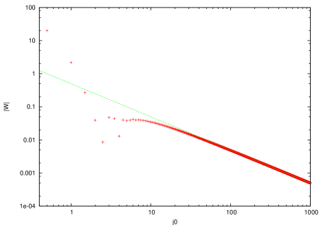
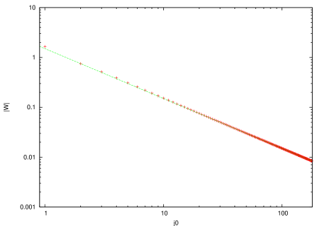
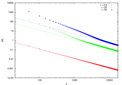
This result can be interpreted as the contribution from a single tetrahedron to the free propagator $\frac{e^{i\omega T}}{2\omega}$, with $\omega\simeq\frac{8}{3j_{0}}$ (see Io ), and it is supported by numerical calculations, reported in Fig.3 below.

The scheme of the perturbative expansion leading to this free propagator can be summarised in the following box:

4 6 11 9 13$+\ldots$ quantum gravity ${\longrightarrow}$ Regge path integral ${\longrightarrow}$ linearised theory

From the scheme above, it should be clear that we have two sources of corrections to 13:

1. contributions coming from higher orders in the expansion of the Regge action and the measure;

2. contributions coming from higher orders in the expansion of the $\{6j\}$ symbol.

We will keep this notation (i) and (ii) throughout the rest of the paper. Corrections (i) come from the non–linear structure of the Regge path integral; whereas the background measure and the quadratic action provide the $1/j_{0}$ behaviour, non trivial contributions from the measure and higher orders in the expansion 9 of the Regge action provide corrections in higher powers of $\ell_{\rm P}$. Because of their origin, these corrections can be considered as the discrete analogues of the QFT self–energies.

On the other hand, (ii) are new kind of corrections, arising from deviations of the $\{6j\}$ symbol from the asymptotics 6; these corrections have no QFT analogues, and cannot be guessed by discretising GR à la Regge. In other words, the microscopic discrete geometry, and its non–Regge like dynamics, does affect the large scale behaviour in a non–trivial way. In particular, we show below that (ii) does not contribute to the NLO, but arises only at the NNLO.

An important remark should be added here. The boundary state $\Psi_{0}[j]$ in 4 is in principle the vacuum state of the full theory, just as the $\{6j\}$ is the kernel of the full theory. In computing the free propagator above, we assumed the Gaussian form 5. However, when computing the corrections to the free propagator, we expect contributions from $\Psi_{0}[j]$ beyond 5. At the present state of investigation, the exact form of the boundary state is not fully understood, thus in the following we discard these terms. See also the comments at the end of Section V.

III.2 NLO: contributions from the Regge action

Let us begin by studying the corrections of type (i); namely, we start from the Regge path integral 11 and study the corrections arising from the measure and terms higher than quadratic in 9. To make the following calculations clearer, let us rewrite 11 collecting the quadratic terms in the exponent,

$$W_{1122}(j_{0})=\frac{1}{j_{0}^{4}}\,\frac{1}{\cal N}\sum_{j_{1},j_{2}}F(j_{0},\delta j_{1},\delta j_{2})\,\exp\left\{-\frac{1}{2}\sum A_{ik}\delta j_{i}\delta j_{k}\right\},$$ (14)

where we have introduced the shorthand notation

$$F(j_{0},\delta j_{1},\delta j_{2}):=\mu(j_{e})\prod_{i}\,[C^{2}(j_{i})-C^{2}(j_{0})]\exp\left\{-i\sum_{a+b\geq 3}^{\infty}\frac{1}{a!b!}\,M_{ab}\,\delta j_{1}^{a}\,\delta j_{2}^{b}\right\},$$ (15)

and we have absorbed a constant factor $\exp\{-i4\,\vartheta\,(j_{0}+\frac{1}{2})\}$ in the normalisation. The normalisation is obtained by taking the same sum in 14 and substituting $F(j_{0},\delta j_{1},\delta j_{2})$ with

$$F_{\cal N}(j_{0},\delta j_{1},\delta j_{2}):=\mu(j_{e})\exp\left\{-i\sum_{a+b\geq 3}^{\infty}\frac{1}{a!b!}\,M_{ab}\,\delta j_{1}^{a}\,\delta j_{2}^{b}\right\}.$$ (16)

Using the explicit values of $\alpha$ given above and of the second derivatives of the Regge action reported in the Appendix, the quadratic exponent can be shown to be

$$A_{ik}=\alpha\delta_{ik}+i\frac{\partial^{2}S_{\rm R}}{\partial j_{i}\partial j_{k}}{\Big{|}_{j_{e}=j_{0}}}=\frac{4}{3j_{0}}\left(\begin{array}[]{cc}1+i\cot\vartheta&-\frac{i}{\sin\vartheta}\\ \\ -\frac{i}{\sin\vartheta}&1+i\cot\vartheta\end{array}\right).$$ (17)

In the following calculations, we will need the inverse of this matrix, which is

$$A^{-1}_{ik}=\frac{3j_{0}}{8}\left(\begin{array}[]{cc}1&e^{i\vartheta}\\ \\ e^{i\vartheta}&1\end{array}\right),$$ (18)

where $e^{i\vartheta}=-\frac{1}{2}+i\sqrt{2}$. All of our analytic calculations will keep track of this simple algebraic form.

The fact that the dominant term in the exponent is quadratic suggests that we can evaluate the sums 14 by approximating them with Gaussian integrals. In fact, in the large $j_{0}$ regime, we have $\sum_{j_{i}=0}^{2j_{0}}\sim\int_{0}^{2j_{0}}dj_{i}=\int_{-j_{0}}^{j_{0}}d\delta j_{i}.$ As is well known,

$$\int_{-\infty}^{\infty}dx\,e^{-\frac{1}{2j_{0}}x^{2}}-\int_{-j_{0}}^{j_{0}}dx\,e^{-\frac{1}{2j_{0}}x^{2}}\sim e^{-\sqrt{j_{0}}},$$ (19)

thus approximating the sums with Gaussian integrals does not affect the NLO of 14. At this point, the logic to study the NLO order in $j_{0}$ is clear: we expand 15 and 16 in powers of $\delta j_{1}$ and $\delta j_{2}$, and then we evaluate the integrals as momenta of Gaussians. If we expand 15, we get

$$F(j_{0},\delta j_{1},\delta j_{2}) = \frac{1}{\sqrt{V}_{0}}\left[(2j_{0}+1)^{4}\delta j_{1}\delta j_{2}+(2j_{0}+1)^{3}\frac{10j_{0}+11}{4(j_{0}+1)}(\delta j_{1}\delta j_{2}^{2}+\delta j_{1}^{2}\delta j_{2})+\right.$$ (20)

$$\left.+(2j_{0}+1)^{2}\frac{(84j_{0}^{2}+124j_{0}+57)}{32(j_{0}+1)^{2}}(\delta j_{1}\delta j_{2}^{3}+\delta j_{1}^{3}\delta j_{2})+(2j_{0}+1)^{2}\frac{116j_{0}^{2}+236j_{0}+125}{16(j_{0}+1)^{2}}\delta j_{1}^{2}\delta j_{2}^{2}+\ldots\right]\times$$

$$\left[1-i\sum_{a+b=3}^{\infty}\frac{1}{a!b!}\,M_{ab}\,\delta j_{1}^{a}\,\delta j_{2}^{b}-\frac{1}{2}\left(\sum_{a+b=3}^{\infty}\frac{1}{a!b!}\,M_{ab}\,\delta j_{1}^{a}\,\delta j_{2}^{b}\right)^{2}+\ldots\right].$$

The structure of this expansion is rather intricate, because the coefficients go down as $j_{0}\mapsto\infty$, whereas the integrals (approximating the sums) go up. In more detail, we have that on the one hand, the coefficients of $\delta j_{i}^{k}$ in the expansion of the measure go as $\frac{1}{\sqrt{V_{0}}}j_{0}^{6-k}$, and $M_{ab}\sim j_{0}^{1-a-b}$; on the other hand, because the squared width of the Gaussian, and thus the values of the squared momenta, are proportional to $j_{0}$, each factor $\delta j_{i}^{2}$ in the integrand contributes a factor $j_{0}$ after the integration is performed. By inspecting 20, we see that the leading term is of the form $j_{0}^{5}/\sqrt{V_{0}}$, and it comes from the first term in both the expansion of the measure and the integral. The next to leading is of the form $j_{0}^{4}/\sqrt{V_{0}}$, and it has a number of contributions: terms up to the fourth order in the expansion of the measure, together with the first, second (with $a+b=3,4$) and third (with $a+b=3$) terms in the expansion of the exponential contribute. Namely, terms up to the fourth order in the expansion of both the measure and the Regge action enter the NLO.

The same analysis for the expansion of the normalisation $\cal N$ shows that we need only the second order in the expansion of the measure, and still the fourth in the expansion of the action,

$$F_{\cal N}(j_{0},\delta j_{1},\delta j_{2}) \simeq \frac{1}{\sqrt{V}_{0}}\left[(2j_{0}+1)^{2}-\frac{1}{2}(2j_{0}+1)(\delta j_{1}+\delta j_{2})+\frac{17}{8}(\delta j_{1}^{2}+\delta j_{2}^{2})+\frac{5}{4}\delta j_{1}\delta j_{2}\right]\times$$ (21)

$$\left[1-i\sum_{a+b=3,4}\frac{1}{a!b!}\,M_{ab}\,\delta j_{1}^{a}\,\delta j_{2}^{b}-\frac{1}{2}\left(\sum_{a+b=3}\frac{1}{a!b!}\,M_{ab}\,\delta j_{1}^{a}\,\delta j_{2}^{b}\right)^{2}\right].$$

At this point, we evaluate separately the Gaussian integrals in the numerator and in the denominator. We then collect all terms in decreasing powers of $j_{0}$, thus obtaining the following structure,

$$W_{1122}(j_{0})=\frac{1}{j_{0}^{4}}\frac{b_{1}j_{0}^{5}+b_{2}j_{0}^{4}+\ldots}{B_{1}j_{0}^{2}+B_{2}j_{0}+\ldots}=\frac{1}{B_{1}}\left[\frac{b_{1}}{j_{0}}+\frac{1}{j_{0}^{2}}(b_{2}-\frac{B_{2}}{B_{1}}b_{1})+\ldots\right].$$ (22)

In particular, $b_{1}=\frac{3e^{i\vartheta}}{2\sqrt{\det A}}$, $B_{1}=\frac{1}{\sqrt{\det A}}$, and $\frac{b_{1}}{B_{1}}$ gives the LO 13 discussed in the previous Section. The NLO can be now computed to be

$$W_{1122}^{\rm\scriptscriptstyle NLO(i)}=-\frac{1}{j_{0}^{2}}\frac{7481-i1048\sqrt{2}}{5184}=-\frac{1}{j_{0}^{2}}(1.4431-i0.2859),$$ (23)

where we have again used $\vartheta=\arccos(-\frac{1}{3})$. The main point to remember is that this is the contribution to the NLO coming from corrections of type (i).

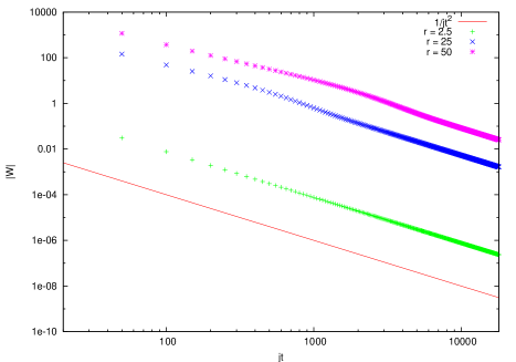
To support this analytic calculation, we fit the NLO using the numerical evaluation of the exact formula 4, and subtracting the fit for the LO 13. The result of the fit is a behaviour $1/{j_{0}^{2}}$ with numerical coefficient ${-1.4431+i0.2860}$ (see Fig.3). This matches our analytic calculation up to three digits. Therefore, there is room for corrections of type (ii) at NLO only if these are very small, of magnitude $10^{-4}$.

Figure 3: The plots showing the numerical evaluation of the 2-point function. Left plot: the leading order. In red, the numerical evaluations of 4; the dashed green line is the analytic result 13. Right plot: the leading order is plotted again, this time together with the next to leading order. The numerical evaluations of the latter is in blue, whereas the analytic result 23 is the red dashed line.

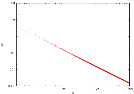
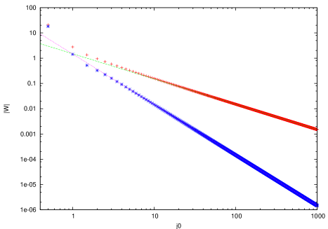
III.3 NLO: contributions from the $\{6j\}$

We now consider (ii), the contribution coming from higher orders in the asymptotics of the $\{6j\}$ symbol 6. From the considerations at the end of the previous Section, we know that if these corrections are present, they are indeed very small. We begin the investigation by studying numerically the next term in the asymptotics of the $\{6j\}$ symbol for the equilateral case, when all spins are $j_{0}$ and $S_{\rm R}[j_{0}]=6(j_{0}+\frac{1}{2})\vartheta$. We use the following ansatz,

$$\left\{\begin{array}[]{ccc}j_{0}&j_{0}&j_{0}\\ j_{0}&j_{0}&j_{0}\end{array}\right\}=\frac{1}{2^{1/4}\sqrt{\pi}\,j_{0}^{3/2}}\cos\left(S_{\rm R}[j_{0}]+\frac{\pi}{4}\right)+\frac{a_{2}}{j_{0}^{5/2}}\cos\left(S_{\rm R}[j_{0}]+\varphi\right)+o({j_{0}^{-\frac{5}{2}}}),$$ (24)

and we perform a two parameters fit, finding the values $a_{2}=-0.3575$, $\varphi=0.6843$. The good performance of this fit suggests the simple ansatz

$$\frac{a_{2}}{(6\sqrt{2})^{\frac{5}{6}}}\frac{\cos\left(S_{\rm R}[j_{1},j_{2},j_{0}]+\varphi\right)}{V(j_{1},j_{2},j_{0})^{\frac{5}{6}}}$$ (25)

as the second term in the expansion 6. If we assume this ansatz, we see that the second term in the asymptotics goes as $j_{0}^{-5/2}$. This is just one power below the first term, thus in principle we should expect the second term of the asymptotics to contribute to the NLO of $W_{1122}(j_{0})$, which is precisely one power below the LO. Notice also that $a_{2}$ is of the same magnitude as $\frac{1}{2^{1/4}\sqrt{\pi}}\sim 0.4744$, so that if the second term does contribute to the NLO, it will do so with the same magnitude as the contribution (i). However, we know that there is no room for this, as the value computed from (i) already matches the exact numerical value up to $10^{-4}$.

We conclude that corrections coming from the second term do not enter the NLO, i.e.

$$W_{1122}^{\rm\scriptscriptstyle NLO}\equiv W_{1122}^{\rm\scriptscriptstyle NLO(i)}.$$ (26)

Understanding the exact way this happens would require a more complete study of the second term in 24, which is beyond the scope of this paper.

IV NNLO: the pure quantum gravity effects

To study the NNLO, we proceed as in the previous section. We first compute analytically the corrections of type (i) coming from expanding the measure and the action, and we then compare the result with the numerical fit obtained from 4, to see if corrections of type (ii) enter. The analytic calculations can be performed as above, thus we do not report here the somewhat tedious details. However, the complexity of the calculations grows as the number of contributions increases largely with every order; we notice that for the NNLO, in the expansion 20, we need up to the eighth derivative in the expansion of the measure, and up to the sixth derivative in the Regge action (namely $a+b\leq 6$); similarly, we need up to the sixth derivative in both the measure and the action in the expansion of $F_{\cal N}$. The result we obtain is

$$W_{1122}^{\rm\scriptscriptstyle NNLO(i)}=\frac{1}{j_{0}^{3}}\frac{62758+i127789\sqrt{2}}{248832}\simeq\frac{1}{j_{0}^{3}}(0.2522+i0.7263).$$ (29)

As expected, the NNLO is one power below the NLO. Notice that the magnitude of the real part is one order of magnitude smaller than the NLO, and the magnitude of the imaginary part same order. This is going to be changed by (ii), the corrections coming from the quantum gravity kernel.

As before, we now evaluate numerically the NNLO, by subtracting 13 and 23 to 4. The best fit gives

$$W_{1122}^{\rm\scriptscriptstyle NNLO(tot)}=W_{1122}^{\rm\scriptscriptstyle NNLO(i)}+W_{1122}^{\rm\scriptscriptstyle NNLO(ii)}\simeq\frac{1}{j_{0}^{3}}(-0.0225+i0.0730).$$ (30)

This fit is quite different from 29, which means that the corrections (ii) do enter the NNLO. Notice that, as expected from 24, (i) and (ii) are of the same magnitude. What is remarkable, is that (ii) have the neat effect of reducing the magnitude of the correction. At this point it becomes interesting to evaluate analytically the second order in 24, and then compute exactly the NNLO coming from it, $W_{1122}^{\rm\scriptscriptstyle NNLO(ii)}$. We leave this issue open for further development.

Let us now use this result to draw some conclusions. Our analysis of the NLO has pointed out that it arises only from higher order corrections in 11. Namely, the NLO is a result of the Regge path integral alone, and is not sensitive to deviations arising from the spinfoam quantum geometry. The latter, on the other hand, are important at NNLO, where they contribute with the same order of magnitude as the Regge–like corrections, but with opposite sign, so that the total NNLO coefficient is smaller than that of the NLO. The structure of the corrections is summarized as follows:

It would be very interesting if a similar structure emerges in 4d as well. To this regard, we conclude this section with a speculative remark. It has been argued that background independent approaches could be the key to avoid the non–renormalisability of GR. The PR model considered here is one such approach, and 3d GR, if treated perturbatively by expanding $g_{\mu\nu}=\eta_{\mu\nu}+h_{\mu\nu}$, suffers the same infinities as the 4d case (in a gauge where $h_{\mu\nu\neq 0}$). Thus, it makes sense to address this idea within the 3d case. In a discretised picture, the conventional perturbative framework is equivalent to using only the Regge path integral, namely starting our computations from 11. So, in a sense, the perturbative expansion that includes only corrections of type (i) is the discrete equivalent of the conventional non–renormalisable perturbative expansion. However, because we did not start from 11, but from the exact background independent quantity 4, we find that new corrections will come in at higher orders, thus changing the structure of the perturbative expansion. Could this provide a possible mechanism for renormalisability? It is very speculative to say so, however we find it intriguing that the new corrections enter at NNLO, precisely where the non–renormalisability of GR shows up.

V On the boundary state

As should be clear from the calculations above, the boundary state plays a key role for the extraction of the inverse power law behaviour, thus it is important to motivate the choice 5. In principle, the boundary state should be given by the vacuum state of the full quantum theory; however, such a state is not known in LQG. To overcome this lack of knowledge, one can proceed with an ansatz. To compute the free propagator, in RovelliProp it was proposed to take, as the vacuum state for the linearised theory, a Gaussian state peaked around the values of the labels for both the intrinsic and the extrinsic geometry of a chosen background, by analogy with quantum mechanics. This suggestion is realized in 3d by 5. Indeed, we can think of it as a state for a quantum mechanical system of conjugate variables $j$ and $\phi$, representing discretized intrinsic and extrinsic geometry. Then, the main property satisfied by 5 is to peak the values of those variable around, respectively, $j_{0}$ and $\vartheta$, and to minimize, in the limit $j_{0}\mapsto\infty$, the relative uncertainties $\frac{\langle{\Delta j}\rangle}{\langle{j}\rangle}$ and $\frac{\langle{\Delta\phi}\rangle}{\langle{\phi}\rangle}$. Notice that in order for this last property to be true, it is crucial the $1/j_{0}$ dependence of the inverse width $\alpha$.

Below we show how this construction can be made more precise, by looking at $j$ and $\phi$ as conjugate variables as defined by the Fourier transform on the structure group of the PR model. Before doing that, we discuss some interesting aspects of the phase term in 5.

V.1 The phase term

We start our investigation by noting an important fact: it is the phase term of 5,

$$\Phi_{\vartheta}(j)=e^{i(j+\frac{1}{2})\vartheta},$$ (31)

that is mainly responsible for the $1/j_{0}$ behaviour of the asymptotics. To understand this, recall that the phase term of 5 represents a state whose dihedral angles are peaked around the equilateral configuration. Therefore, the presence of the phase term is enough to expand the Regge action around such a configuration; but since the bulk edges of the tetrahedron are fixed to $j_{0}$, the equilateral configuration is exactly the one used in the calculations in Section III. This means that even if we set $\alpha=0$ in 5, we can proceed consistently with the perturbative expansion as in Section III. The only difference is that now the matrix $A$ in 17 consists only of the second derivatives of the Regge action. Indeed, we find the following analytic result:

$$W_{1122}(j_{0})\simeq\frac{1}{j_{0}}i\frac{9}{2\sqrt{2}}+\frac{1}{j_{0}^{2}}\Big{(}-\frac{245}{64}+i\frac{9}{2\sqrt{2}}\Big{)}.$$ (32)

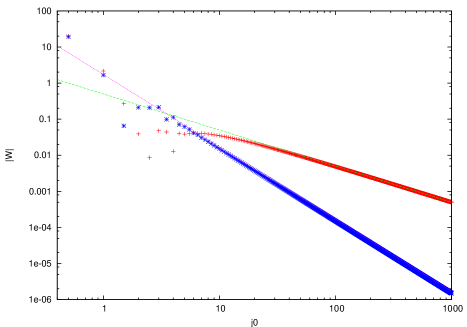
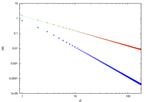
Once again, we support this result with the numerical simulations, which are reported in Fig.4. Notice that we get much more oscillation, due to the absence of the quadratic damping factor.

Figure 4: The plots showing the numerical evaluation of the 2-point function with $\alpha=0$. Left plot: the leading order. In red, the numerical evaluations of 4; the dashed green line is the analytic result in 32. Right plot: the numerical evaluations of the next to leading order, in blue, together with the first two terms of the analytic result 23. The green dashed line is the leading order, whereas the red dashed line shows the next to leading.

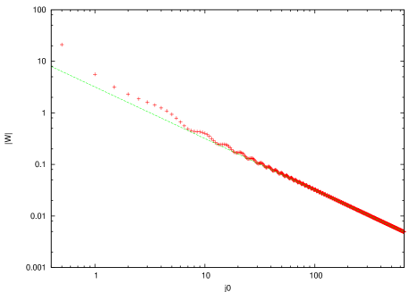
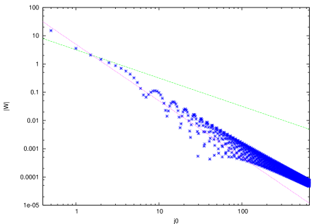
In particular, we see from the right figure that the NLO oscillates quite strongly, and this makes it hard to fit its value. Of course, 5 with $\alpha=0$ loses the semiclassical properties described above, however, this is just an exercise to show that actually is the phase term the key object, as much as the calculations are concerned.

The fact that the phase term alone is sufficient to get the right leading–order asymptotic behaviour, suggests that we have freedom in choosing the angle: with $\alpha=0$, different angles would still give non trivial results. Indeed, these would correspond to non equilateral geometric configurations (see Section VII below).

The phase term has another interesting property. By inspecting 4, we see that it is the only $\mathbbm{C}$-valued quantity entering the definition of the 2-point function; thus, it is responsible for the 2-point function being a complex quantity. Recall that we are working in a measured–time setting, where the 2-point function is reconstructed as $\frac{e^{i\omega T}}{2\omega}$, so a complex result is what we need in order to be consistent with this interpretation. However, one can also consider a different setting, where all boundary edges are allowed to fluctuate. This “general boundary” context is particularly relevant in the 4d case model discussed in RovelliProp , where the measured–time setting is not applicable. In the general boundary context, one expects to reconstruct the 2-point function in configuration space; in the Riemannian case, a real function of the spacetime distance between the points, so that the computation of the 2-point function has to lead to a real result. This is not obvious, if the phase term is $\mathbbm{C}$-valued. In fact, notice that in RovelliProp , the author has to choose a $\mathbbm{C}$-valued (non–diagonal) quadratic term in the Gaussian boundary state, in order to compensate for the complex phase term, and make the final result real. Here, we would like to suggest that the reality of the result can be obtained keeping the simple quadratic Gaussian term, but rather changing the phase to a real quantity. We argue below that this can be done without losing the $1/j_{0}$ behaviour.

The immediate choice to make the phase real is to take either the real or the imaginary part of 31, i.e. $e^{i(j+\frac{1}{2})\vartheta}\pm e^{-i(j+\frac{1}{2})\vartheta}.$ In principle, it is not obvious that such a phase term will still guarantee the $1/j_{0}$ behaviour, thus we find it useful to address this issue within the toy model so far described. To fix ideas, let us choose the real part, and consider a new boundary state in 4 whose phase term is given by $\prod_{i}\cos(j_{i}+\frac{1}{2})\vartheta$. We keep the same quadratic term as in 5, and we use again 6 to study the leading order. This leads to a structure of the type

$$\left(e^{i(j_{1}+\frac{1}{2})\vartheta}+e^{-i(j_{1}+\frac{1}{2})\vartheta}\right)\left(e^{i(j_{2}+\frac{1}{2})\vartheta}+e^{-i(j_{2}+\frac{1}{2})\vartheta}\right)\Big{(}e^{iS_{\rm R}+i\frac{\pi}{4}}+e^{-iS_{\rm R}-i\frac{\pi}{4}}\Big{)}.$$ (33)

Recall that the linear order of the Regge action is $[4(j_{0}+\frac{1}{2})+j_{1}+j_{2}+1]\vartheta$. As discussed in Section III, only the exponential of the Regge action when the linear term is cancelled will contribute to the 2-point function, the other term being negligible due to the oscillations in the sum. It is thus clear that taking the cosine as the phase term makes in principle both exponentials of the Regge action matter. However, attention must be paid to the factor $4(j_{0}+\frac{1}{2})\vartheta$ in the linear order of the Regge action. In Section III we were able to discard the related phase $e^{-i4(j_{0}+\frac{1}{2})\vartheta}$, by reabsorbing it in the normalisation. This can not be done now, because both orientations matter. Including also the normalisation, we indeed have

$$W_{1122}(j_{0}) = \frac{1}{j_{0}^{4}}\frac{e^{-i4(j_{0}+\frac{1}{2})\vartheta-i\frac{\pi}{4}}\left[b_{1}j_{0}^{5}+\ldots\right]+e^{i4(j_{0}+\frac{1}{2})\vartheta+i\frac{\pi}{4}}\overline{\left[b_{1}j_{0}^{5}+\ldots\right]}}{e^{-i4(j_{0}+\frac{1}{2})\vartheta-i\frac{\pi}{4}}\left[B_{1}j_{0}^{2}+\ldots\right]+e^{i4(j_{0}+\frac{1}{2})\vartheta+i\frac{\pi}{4}}\overline{\left[B_{1}j_{0}^{2}+\ldots\right]}}=$$ (34)

$$= \frac{1}{j_{0}^{4}}\frac{{\rm Re}\left[b_{1}j_{0}^{5}+\ldots\right]+{\rm Im}{\left[b_{1}j_{0}^{5}+\ldots\right]}\tan{\left[4(j_{0}+\frac{1}{2})\vartheta+i\frac{\pi}{4}\right]}}{{\rm Re}\left[B_{1}j_{0}^{2}+\ldots\right]+{\rm Im}{\left[B_{1}j_{0}^{2}+\ldots\right]}\tan{\left[4(j_{0}+\frac{1}{2})\vartheta+i\frac{\pi}{4}\right]}}.$$

While the first terms of numerator and denominator would produce the right $1/j_{0}$ behaviour, we see that we have an extra $j_{0}$-dependent phase which spoils the result. Therefore, the choice $\prod_{i}\cos(j_{i}+\frac{1}{2})\vartheta$ does not work. It is easy to see that this problem can be fixed by taking

$$\Phi_{\vartheta}(j_{i})=\cos(j_{i}+2j_{0}+\frac{3}{2})\vartheta,$$ (35)

so that the linear term of the Regge action is exactly cancelled. In this way we get

$$W_{1122}(j_{0})=\frac{1}{j_{0}^{4}}\frac{{\rm Re}\left[b_{1}e^{-i\frac{\pi}{4}}j_{0}^{5}+\ldots\right]}{{\rm Re}\left[B_{1}e^{-i\frac{\pi}{4}}j_{0}^{2}+\ldots\right]}$$ (36)

Indeed, this latter choice cancels all $j_{0}$-dependent phases, and the $1/j_{0}$ behaviour is restored. In particular, using the same quadratic term as in 5, we obtain the same $b_{1}$ and $B_{1}$ of 22, and thus the LO of 36 is

$$W_{1122}(j_{0})\,=\,\frac{1}{j_{0}}\left(\frac{{\rm Re}\,b_{1}+{\rm Im}\,b_{1}}{{\rm Re}\,B_{1}+{\rm Im}\,B_{1}}\right)\,=\,\frac{3\sin\frac{3}{2}\vartheta}{2j_{0}\sin\frac{\vartheta}{2}}=\frac{1}{2j_{0}}.$$ (37)

This result is indeed supported by the numerics (see Fig.5). Therefore, it is possible to keep the simple diagonal and real quadratic term in the boundary state, and choose a phase term such that the 2-point function is a real quantity at all orders, with leading order proportional to $1/j_{0}$.

Figure 5: The plots for the real boundary state 35. Left plot: the leading order. In red, the numerical evaluations; the dashed green line is the analytic result in 37. Right plot: the numerical evaluations of the next to leading order, in blue, together with the analytic result of the next to leading in 37.

However, let us stress that this construction is not physically interesting in the measured–time setting, where the 2-point function is a complex function, as mentioned above. This is reflected in the fact that 35 is not a sensible choice for the phase term: the boundary is defined on the hyperplanes and it should not refer to the bulk edges. On the other hand, the interest in the computation performed above is to have an exploratory investigation towards the general boundary context. In fact, in the general boundary setting, all edges $e$ of the tetrahedron are allowed to fluctuate, thus it makes sense to take $\prod_{e}\cos(j_{e}+\frac{1}{2})\vartheta$ as the phase term of the boundary state. Since this quantity contains a phase that cancels exactly the linear order of the Regge action, we expect its use to give a real $1/j_{0}$ behaviour. The calculation performed here supports the idea that such a choice would give a correct real 2-point function. In the measured–time setting, the only interest in 35 is to show that using a real phase term would still work, with the benefit of a real 2-point function.

We conclude with a remark about choosing the imaginary part of 31. Because of the normalisation in 4, this is equivalent to take the $\mathrm{SU}(2)$ character itself, i.e.

$$\Phi_{\vartheta}(j)=\chi_{j}(\frac{\vartheta}{2})=\frac{e^{i(j+\frac{1}{2})\vartheta}-e^{-i(j+\frac{1}{2})\vartheta}}{2i\sin\frac{\vartheta}{2}}.$$ (38)

It is interesting to note that 38 can be interpreted as the propagator of a point particle coupled to the PR model etera . Consequently, the use of 38 as the phase term of the boundary state opens the way to a new possible interpretation of the gauge–fixing performed in this computation: 37 can be thought of as the 2-point function in the gauge fixed by the presence of a particle in the boundary.

V.2 Harmonic analysis

We parametrise $\mathrm{SU}(2)$ elements as

$$g(\phi,\hat{n})=\cos\frac{\phi}{2}\,\mathbbm{1}+i\,\sin\frac{\phi}{2}\,\hat{n}\cdot\vec{\sigma},\quad\phi\in[0,4\pi[,\quad\hat{n}\in{\cal S}^{2},$$

where $\sigma_{i}$ are the Pauli matrices, satisfying $\sigma_{i}^{2}=\mathbbm{1}$. Moreover, the group element $g(\phi,\hat{n})$ is obviously identified to $g(-\phi,-\hat{n})$. We can thus restrict $\phi$ to live in $[0,2\pi]$. Finally, $g(\phi,\hat{n})$ and $g(\phi+2\pi,\hat{n})\,=\,-g(\phi,\hat{n})$ actually define the same rotation in the 3d space (same $\mathrm{SO}(3)$ group element). In this representation, the characters and the Haar measure are given respectively by:

$$\chi_{j}(g)=\frac{\sin(j+\frac{1}{2})\phi}{\sin\frac{\phi}{2}},\qquad dg=\frac{1}{4\pi^{2}}\sin^{2}\frac{\phi}{2}\,d^{2}\Omega(\hat{n})\,d\phi.$$

A class function $f$ is a function on the group which is invariant under conjugate action, $f(g)=f(hgh^{-1})$. With the parametrisation chosen above, it is a function of the angle $\phi$ only. For such a function, the Fourier transform can be simply written as $f(g)=\sum_{j}\hat{f}_{j}\,\chi_{j}(g)$, with $\hat{f}_{j}=\int dg\,f(g)\,\chi_{j}(g)$. If $j$ and $\phi$ in 5 are conjugate variable like this, then just as 5 is a Gaussian peaked around $j_{0}$ in the irrep labels basis, then its Fourier transform should describe a Gaussian on the group peaked around the class element $\vartheta$. However, in spite of its simple structure, 5 does not admit a simple Fourier transform. For, in the limit $j_{0}\mapsto\infty$, we can approximate the sum with integrals, and find:

$$\widetilde{\Psi}_{0}(\phi) = \sum_{j}\Psi_{0}(j)\,{\chi_{j}(\phi)}=\sum_{j}e^{-\frac{\alpha}{2}(j-j_{0})^{2}+i(j+\frac{1}{2})\vartheta}\,{\chi_{j}(\phi)}$$ (39)

$$\simeq \sqrt{\frac{\pi}{2\alpha}}\frac{1}{2i\sin\frac{\phi}{2}}\,\left[e^{i(j_{0}+\frac{1}{2})(\vartheta+\phi)}e^{-\frac{1}{2\alpha}(\phi+\vartheta)^{2}}-e^{i(j_{0}+\frac{1}{2})(\vartheta-\phi)}e^{-\frac{1}{2\alpha}(\phi-\vartheta)^{2}}\right].$$

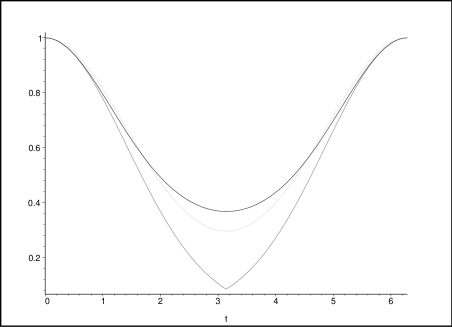
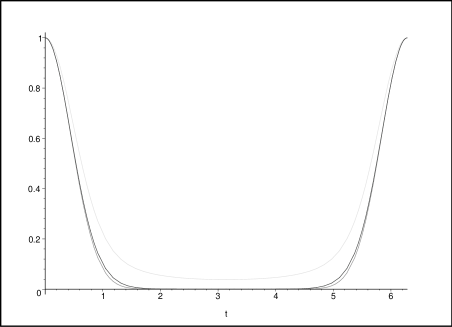
However, notice that a function of the type $e^{-\frac{1}{2\alpha}\phi^{2}}$ is not smooth (or even continuous) on $\mathrm{SU}(2)$. This is due to the compactness of $\mathrm{SU}(2)$ and the gluing condition at the “boundary” $\phi\,=\,0\,[2\pi]$.

A smooth, more natural Gaussian–like function on $\mathrm{SU}(2)$ would be

$$\widetilde{\psi}_{0}(g)=\frac{1}{N^{\prime}}e^{\frac{1}{2\alpha}{\rm Tr}(g\cdot\vec{\sigma})^{2}}=\frac{1}{N^{\prime}}e^{-\frac{2}{\alpha}\sin^{2}\frac{\phi}{2}},$$ (40)

where the trace Tr is taken in the fundamental $j=1/2$ irrep. This function can be easily decomposed into its Fourier modes; notice in fact that ${\rm Tr}(g\cdot\vec{\sigma})^{2}=\chi_{\frac{1}{2}}^{2}(g)-4$, thus 40 can be expanded in a simple sum of characters, thanks to the decomposition property of tensor products into irreps, $\chi_{\frac{1}{2}}^{n}=\sum_{j}c_{j}\chi_{j}$. This feature makes it a more natural object to use within the group structure of $\mathrm{SU}(2)$. For a comparison with 39, see Fig.6.

Figure 6: We plot the three considered Gaussian distributions on $\mathrm{SU}(2)$ peaked around $\pm\mathbbm{1}$: $f_{1}(\phi)=e^{-\frac{2}{\alpha}\sin^{2}\frac{\phi}{2}}$, $f_{2}(\phi)=\sum_{j}\chi_{j}(\phi)e^{-\frac{\alpha}{2}j^{2}}$ and $f_{3}(\phi)=e^{-\frac{1}{2\alpha}\phi^{2}}$ (for $\phi\in[0,\pi]$ and its mirror image $e^{-\frac{1}{2\alpha}(2\pi-\phi)^{2}}$ for $\phi\in[\pi,2\pi]$). The two plots respectively correspond to the values $\alpha=2$ and $\alpha=0.2$. On the first plot, it is clear that the three Gaussians are distinct and that $f_{3}$ is not smooth. On the second, we see that $f_{2}$ converges toward the distribution $f_{3}$ as $\alpha$ goes to 0 (high $j_{0}$), thus justifying 39 while the distribution $f_{1}$ dual to the Bessel functions remains slightly different. This deviation of $f_{1}$ from the standard $f_{2}$ will be responsible for the different NLO of the 2-point function when using it as boundary state (see below).

To find the normalisation $N^{\prime}$, we evaluate the integral

$$|N^{\prime}|^{2}=\int_{\mathrm{SU}(2)}dg\,e^{\frac{1}{\alpha}{\rm Tr}(g\cdot\vec{\sigma})^{2}}=\frac{1}{\pi}\int_{0}^{2\pi}d\phi\,\sin^{2}\frac{\phi}{2}\,e^{-\frac{4}{\alpha}\sin^{2}\frac{\phi}{2}}=e^{-\frac{2}{\alpha}}\left[I_{0}(\frac{2}{\alpha})-I_{1}(\frac{2}{\alpha})\right],$$ (41)

where $I_{n}(\frac{1}{\alpha})$, $n\in\mathbbm{N}$, are the modified Bessel functions of the first kind (see the Appendix). In a similar way, we can compute the Fourier transform of 40. For $j\in\mathbbm{N}$, we have

$$\psi_{0}(j)=\int_{\mathrm{SU}(2)}dg\,\widetilde{\psi}_{0}(g)\,\chi_{j}(g)=\frac{1}{N^{\prime}}\frac{1}{\pi}\int_{0}^{2\pi}d\phi\,\sin\frac{\phi}{2}\,\sin(2j+1)\frac{\phi}{2}\,e^{-\frac{2}{\alpha}\sin^{2}\frac{\phi}{2}}=\frac{I_{j}(\frac{1}{\alpha})-I_{j+1}(\frac{1}{\alpha})}{\sqrt{I_{0}(\frac{2}{\alpha})-I_{1}(\frac{2}{\alpha})}},$$ (42)

where we used the explicit value 41. On the other hand, $\psi_{0}(j)$ vanishes if $j$ is strictly an half–integer.

At first sight, it is not obvious that 42 fulfills the semiclassical properties required earlier. However, as we show in the Appendix, the $\alpha\mapsto 0$ limit of 42 is $\sqrt{2}\sqrt[4]{\frac{\alpha}{\pi}}e^{-\frac{\alpha}{2}j^{2}}$, namely a Gaussian peaked around $j=0$. We are on the right track. To obtain a function peaked around $j_{0}$, we need to shift the peak. This can be done in a simple way, now that we understand the Gaussian in the irrep label basis as the Fourier transform of 40; to shift the peak of the Gaussian to a value $j_{0}$, it is enough to multiply 40 by the appropriate Fourier mode, namely $\chi_{j_{0}}(g)$. Accordingly, we consider the following function,

$$\widetilde{\psi}_{0}(g)=\frac{1}{N}e^{\frac{1}{2\alpha}{\rm Tr}(g\cdot\vec{\sigma})^{2}}\chi_{j_{0}}(g),\qquad N=e^{-\frac{1}{\alpha}}\sqrt{I_{0}(\frac{2}{\alpha})-I_{2j_{0}+1}(\frac{2}{\alpha})}.$$ (43)

Proceeding as above and using $\chi_{j}(g)\,\chi_{j_{0}}(g)=\sum_{k}\chi_{k}(g)$, it is straightforward to check that the Fourier transform of 43 is

$$\psi_{0}(j)=\frac{1}{N}\sum_{k=|j-j_{0}|}^{j+j_{0}}\int_{\mathrm{SU}(2)}dg\,e^{\frac{1}{2\alpha}{\rm Tr}(g\cdot\vec{\sigma})^{2}}\chi_{k}(g)=\frac{I_{|j-j_{0}|}(\frac{1}{\alpha})-I_{j+j_{0}+1}(\frac{1}{\alpha})}{\sqrt{I_{0}(\frac{2}{\alpha})-I_{2j_{0}+1}(\frac{2}{\alpha})}}.$$ (44)

Again, this result holds for $j$ integer, whereas $\psi_{0}(j)$ vanishes for $j$ strictly an half–integer. For small $\alpha$, this is approximated by (see the Appendix)

$$\psi_{0}(j)\simeq\frac{I_{|j-j_{0}|}(\frac{1}{\alpha})}{\sqrt{I_{0}(\frac{2}{\alpha})}}\simeq\sqrt{2}\sqrt[4]{\frac{\alpha}{\pi}}\,e^{-\frac{\alpha}{2}(j-j_{0})^{2}},$$ (45)

and it describes a Gaussian peaked around $j_{0}$, with squared width $\frac{1}{\alpha}$, as we wanted.

Let us now discuss the dihedral angle. 43 is a Gaussian peaked around $\phi=0$. We want to shift this peak as well, around $\phi=\vartheta$. This can be done adding a phase in $j$. The simplest way to do so, without spoiling the property of having a simple Fourier transform, is to add to 44 the real phase term $\cos(j+\frac{1}{2})\vartheta$, which we discussed in the previous section. Then, we consider

$$\Psi_{0}(j)=\frac{I_{|j-j_{0}|}(\frac{1}{\alpha})-I_{j+j_{0}+1}(\frac{1}{\alpha})}{\sqrt{I_{0}(\frac{2}{\alpha})-I_{2j_{0}+1}(\frac{2}{\alpha})}}\,\cos(j+\frac{1}{2})\vartheta.$$ (46)

The reason why the cosine is the easier choice to add a phase in $j$ is that using

$$\cos\left[\left(j+\frac{1}{2}\right)\vartheta\right]\,\chi_{j}(\phi)\,=\,\frac{\sin\frac{\phi-\vartheta}{2}}{2\sin\frac{\phi}{2}}\,\chi_{j}(\phi-\vartheta)\,+\,\frac{\sin\frac{\phi+\vartheta}{2}}{2\sin\frac{\phi}{2}}\,\chi_{j}(\phi+\vartheta)$$ (47)

we can simply compute the Fourier transform of 46 shifting the character’s argument as in 47, and we get

$$\widetilde{\Psi}_{0}(g)\,=\,\frac{1}{2N\sin\frac{\phi}{2}}\left[\,\sin(\frac{\phi-\vartheta}{2})\,\chi_{j_{0}}(\phi-\vartheta)\,e^{-\frac{2}{\alpha}\sin^{2}\frac{\phi-\vartheta}{2}}\,+\,\sin(\frac{\phi+\vartheta}{2})\,\chi_{j_{0}}(\phi+\vartheta)\,e^{-\frac{2}{\alpha}\sin^{2}\frac{\phi+\vartheta}{2}}\,\right].$$ (48)

Let us comment on this expression. In the general boundary context, 46 can be taken as a new ansatz for the boundary state. It has a good semiclassical behaviour, in the sense described above: in the $j_{0}\mapsto\infty$ limit, it becomes a Gaussian peaked around $j=j_{0}$ (see 46) and $\phi=\vartheta,\pi-\vartheta$ (see 48). Furthermore, the interpretation of $j_{0}$ and $\vartheta$ as conjugate variables has now a clear mathematical meaning: they are conjugate with respect to the $\mathrm{SU}(2)$ Fourier transform.

Notice that we are led to include also the configuration $\phi=\pi-\vartheta$: the $\mathrm{SU}(2)$ angle $\phi$ represents both the external dihedral angle $\vartheta$ and the internal angle $\pi-\vartheta$ between the triangles. In other words, the boundary spin network has an inside–outside symmetry.

In the general boundary context, we expect the use of 48 to lead to a real propagator $W$ with the correct $1/j_{0}$ leading order. This is suggested by the asymptotics 45. To support this expectation, we consider this new ansatz in the toy model presented in this paper. In our context however, we cannot use the cosine phase term, as we discussed above. Then, we consider 42 for the quadratic term and the the usual phase 31. Choosing the same $\alpha=\frac{4}{3j_{0}}$ as before, we obtain from the numerics exactly the same leading order 13 (see also Fig.7),

$$W_{1122}(j_{0})\simeq\frac{1}{j_{0}}(-0.5+i1.4)+\frac{1}{j_{0}^{2}}(-1.3-i0.2)$$ (49)

Notice that the next to leading order is now different. This is due to the fact that 44 contributes non trivial corrections. Indeed, the leading order of its perturbative expansion, 45, reduces to the quadratic part of 5, but higher order terms enter the calculation of the propagator corrections.

Figure 7: Leading and next to leading orders using 44. Left plot: the leading order. In red, the numerical evaluation; the dashed green line is the analytic result in 32. Right plot: the numerical evaluations of the next to leading order, in blue, together with the leading order plot.

From this point of view, the use of 44 enriches the toy model, and it makes it possible also to consider the most complete structure of the graviton perturbative expansion, where both the kernel and the boundary state are given as a power series in $\ell_{\rm P}$.

As for the contribution of these new corrections, notice that the NLO in 49 is slightly smaller than the NLO 23. This might look like a side result. However, in 4d the numerical complexity grows very fast, a fact that has slowed down numerical computations thus far. Therefore, having a new boundary state which reaches the same asymptotic behaviour earlier could turn out to be very useful, were the same behaviour to hold in 4d. Furthermore, it turns out that using such a boundary state allows an exact calculation of the LO of the 2-point function in the 4d case; namely, one does not need to use the (troubled) asymptotic formula of the $\{10j\}$ symbol, but one can uses its exact expression in terms of integrals of character. A work on this is in preparation noi2 .

VI Comparing different spinfoam models: stability of the leading order

The definition of the $n$-point functions in the spinfoam formalism is not only fundamental to extract physical predictions, it is also important for distinguishing between the different existing models. In particular, obtaining the correct LO for the 2-point function is a requirement for any sensible model. In 4d, there are a variety of different models, and using the equivalent of 4 to study their large scale limit could possibly be a good way to narrow them down. However, some variety is also present for the 3d models, and it is useful to consider the 3d toy model to begin to investigate how different models can produce different 2-point functions.

We consider a simple generalisation of the PR model, where we modify the face weights, by taking

$${\cal A}^{k}_{\Delta}(j_{e})=\prod_{e}(2j_{e}+1)^{k}\prod_{\tau}\left\{6j\right\}_{\tau}$$ (50)

as the amplitude. The original model is reproduced for $k=1$.

From the point of view of the Regge path integral 11, this new definition of the kernel amounts simply to a change in the measure term 12, which becomes

$$\mu_{k}(j_{e}):=\frac{\prod_{i}\,(2j_{i}+1)^{k}}{\sqrt{V(j_{1},j_{2},j_{0})}}.$$ (51)

If we take into account this change, we can straighforwardly recompute the LO and the NLO, and we find that the $k$-dependence enters in a very simple way:

$$W^{k}_{1122}(j_{0})=-\frac{1}{j_{0}}(\frac{1}{2}-i\sqrt{2})-\frac{1}{j_{0}^{2}}(\frac{1}{2}-i\sqrt{2})\frac{1}{2}[k^{2}-\frac{5}{3}k+\frac{2161}{1296}+i(\frac{7}{3\sqrt{2}}k+\frac{17}{648\sqrt{2}})].$$ (52)

Let us comment on this result. Firstly, the LO is insensitive to this kind of modification. This means that any spinfoam model of the type 50 leads to the same asymptotic behaviour of the 2-point function. This result is expected, as we know from the previous analysis that at leading order only the trivial background value for the measure enters, so that any $k$-dependence is washed away by the normalisation in 4.

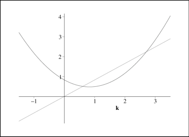
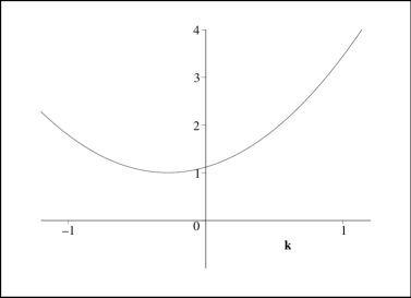
On the other hand, the NLO depends on $k$, thus different models lead to different corrections. While the (conventional) case $k=1$ remarkably minimises the real part of the relative correction $W^{\rm\scriptscriptstyle NLO}/W^{\rm\scriptscriptstyle LO}$ (see left plot of Fig.8), the minimum of the absolute correction is reached for $k=0$, the case of trivial face weights.

Figure 8: The relative correction $W^{\rm\scriptscriptstyle NLO}/W^{\rm\scriptscriptstyle LO}$, as a function of the measure weight $k$. On the left, the case with boundary state 5; the quadratic function is the real part, while the linear function is the imaginary part. We see that $k=1$ is the integer value closest to the minimum of the real part. On the right, the real case with 35 as the phase of the boundary state. We see that $k=0$ is the integer value closest to the minimum.

This feature is clarified if we use 38 as the phase of the boundary state, which leads to a real 2-point funtion. In this latter case, the $k$-dependence of the correction is

$$W^{k}_{1122}(j_{0})=-\frac{1}{2j_{0}}-\frac{1}{j_{0}^{2}}(\frac{3}{4}k^{2}+\frac{5}{12}k+\frac{8701}{15552}),$$ (53)

and we see that the case $k=0$ minimises the correction (see the right plot of Fig.8).

VII Extending the toy model: the isosceles case

In this last section, we want to address a different issue. In the toy model considered so far, we have restricted our attention to the case when the background is chosen to be an equilateral tetrahedron. However, we expect the results here described to extend to a generic background configuration. To give an idea of the way things would work out, and as a first generalisation, we consider in this Section the case when the two opposite edges of the background tetrahedron have spin $j_{0}$, and the four bulk edges have spin $j_{t}$. We call the corresponding dihedral angles $\vartheta_{0}$, $\vartheta_{t}$ (all relevant formulas are reported in the Appendix). In this case, we can still consider an embedding in 3d Euclidean spacetime as in Fig.1, and $T=t_{2}-t_{1}=\frac{1}{\sqrt{2}}{\sqrt{2j_{t}^{2}-j_{0}^{2}}}$.

The physical setting of the problem is exactly the same. The only difference is the geometric analysis, which is now slightly more involved. In particular, notice that not all configurations $(j_{0},j_{t})$ are admissable; since the tetrahedron is embedded in Euclidean spacetime, triangle inequalities must hold, and thus we restrict in the following to $\sqrt{2}j_{t}\geq j_{0}$.

Using the simple ansatz of the type 5 for the boundary state, the expression 4 for the propagator now reads

$$W_{1122}(T)=\frac{1}{j_{0}^{4}}\,\frac{1}{\cal N}\,\sum_{j_{1},j_{2}=0}^{2j_{t}}\left[\prod_{i}\,(2j_{i}+1)\;[C^{2}(j_{i})-C^{2}(j_{0})]\,\Psi_{0}[j_{i}]\right]\left\{\begin{array}[]{ccc}j_{1}&j_{t}&j_{t}\\ j_{2}&j_{t}&j_{t}\end{array}\right\},$$ (54)

with

$$\Psi_{0}[j_{i}]=\exp\left\{-\frac{\alpha}{2}(j_{i}-j_{0})^{2}+i\vartheta_{0}(j_{i}+\frac{1}{2})\right\}$$ (55)

and $\cos\vartheta_{0}=-\frac{4j_{t}^{2}-3j_{0}^{2}}{4j_{t}^{2}-j_{0}^{2}}$ (see the Appendix). To obtain the leading order of 54, we study the limit $(j_{t},j_{0})\mapsto\infty$ with $r=j_{t}/j_{0}$ fixed. This last requirement is necessary in order for 6 to hold; furthermore, it would not be very interesting to study the inhomogeneous limit $j_{t}\mapsto\infty$ with $j_{0}$ fixed, because this means going towards a degenerate configuration where the tetrahedron is squeezed into a 2d surface. In the limit $(j_{t},j_{0})\mapsto\infty$, we proceed as in Section III, using 6 for the $\{6j\}$ symbol, and expanding the Regge action. Choosing the value

$$\alpha=\frac{4r}{j_{0}(4r^{2}-1)}$$ (56)

for the free parameter entering 55, we obtain

$$W_{1122}(j_{t},j_{0})=\frac{1}{j_{0}^{4}}\,\frac{1}{\cal N}\sum_{j_{1},j_{2}}F(j_{0},\delta j_{1},\delta j_{2})\;e^{-\frac{1}{2}\sum A_{ik}\delta j_{i}\delta j_{k}}$$ (57)

with

$$A_{ik}=\frac{j_{0}(4r^{2}-1)}{4r}\left(\begin{array}[]{cc}1+i\cot\vartheta_{t}&-\frac{i}{\sin\vartheta_{t}}\\ \\ -\frac{i}{\sin\vartheta_{t}}&1+i\cot\vartheta_{t}\end{array}\right).$$ (58)

Here we used the fact that $\cos\vartheta_{t}=-\frac{1}{4r^{2}-1}$ (see the Appendix). Once again, this matrix can be interpreted as the kernel for a harmonic oscillator (see for instance carlo , or the appendix of Io ), if we identify the frequency of the oscillator with $\omega=\frac{\vartheta_{t}}{T}.$ Indeed, it is this request that motivated our choice 56.

At leading order, $F(j_{0},\delta j_{1},\delta j_{2})$ can be read from the first term of 20; the analogous term in the normalisation is the first term of 21. Approximating the sums as Gaussian integrals as in Section III, we get

$$W_{1122}(j_{t},j_{0})=\frac{4r^{2}-1}{2j_{t}}e^{i\vartheta_{t}}.$$ (59)

For $r=1$, we recover the equilateral result 13. To consider non equilateral configuration, we plot 59 for different values of $r$.

Figure 9: Exact numerical evaluation of $|W_{1122}|$ as a function of $j_{t}$, for $r=2.5,25,$ and $50$. On the left, the leading order, computed in 59. On the right, the next to leading order, not computed analytically here.

In particular, if $r\gg 1$, we have $\cos\vartheta_{t}\simeq\frac{\pi}{2}$ and $\omega\simeq\frac{\pi}{2rj_{0}}$, and 59 reads

$$W_{1122}(T)\simeq\frac{2\pi}{j_{0}^{2}}\frac{e^{i\omega T}}{2\omega}.$$ (60)

A comparison of the exact numeric calculation with the asymptotics is shown in Figure 9, where we see good agreement with the prediction of 59. Note, however, that the asymptotic value is reached more and more slowly as $r$ increases.

VIII Conclusions and perspectives

We have considered a single tetrahedron embedded in 3d Euclidean spacetime as a toy model to test how the spinfoam formalism can be used to construct the perturbative quantum theory of gravitons. We focused on a single component of the propagator, defined in 4, and computed the NLO and NNLO corrections to the free $1/\ell$ behaviour. These are given respectively in 23 and 29 and, as expected, have the behaviour $1/\ell^{2}$ and $1/\ell^{3}$.

We found that these corrections have an interesting structure. On the one hand, the NLO can be entirely computed from an expression, given in 11, which is a path integral for the Regge action. This can be seen as the discrete analogue of the conventional continuum definition of the 2-point function. On the other hand, the NNLO gets contributions from the true, non Regge–like spinfoam dynamics. This in turn cannot be written down by simply discretizing the GR action à la Regge. Here is where the use of the spinfoam formalism modifies substantially the conventional expansion. It is particularly intriguing that this new source of corrections enters at NNLO, precisely where the continuum theory becomes non renormalisable, and that it reduces the magnitude of the NNLO correction.

We introduced a new ansatz for the boundary state, given in 46, which reduces to the original Gaussian in the large $j$ limit, and thus satisfies the semiclassical requirements, but has the advantage of making $j$ and the dihedral angle conjugate variables with respect to the harmonic analysis over $\mathrm{SU}(2)$. This property helps treating the sums appearing in the evaluation of expectation values within the PR model. In particular in 4d, the Riemannian Barrett–Crane model uses the gauge group $\mathrm{Spin}(4)\sim\mathrm{SU}(2)\times\mathrm{SU}(2)$, to which we can apply all the tools developed here for the gauge group $\mathrm{SU}(2)$. Remarkably, the use of 46 in the general boundary context allows us to write the 4d propagator as an integral over the group noi2 .

It would be interesting to extend these results to the Lorentzian case, using the expression 4 with group $\mathrm{SU}(1,1)$. The $\mathrm{SU}(1,1)$ $\{6j\}$ symbol satisfies the Lorentzian version of the asymptotics 6 asympt , thus we expect to be able to perform the same analysis pursued in this paper for the Riemannian case. It is also worth mentioning that in the non–equilateral Lorentzian case, there are no triangle inequalities to fulfill, thus the analysis is richer.

In light of these results, we think that this approach is very promising: it allows computation of the leading order as well as the corrections of (a component of) the graviton propagator, and, in a more general perspective, of semiclassical observables. When applying this program to 4d, it will be interesting to compare and possibly match the spinfoam corrections to the loop corrections computed in the standard perturbative expansion (see e.g. Donoghue ). Let us nevertheless point out that the NNLO in our 3d model already contains an impressive number of terms and that the technical difficulties to organize and compute further spinfoam corrections will likely be comparable to the ones encountered when computing and summing the Feynman diagrams at two–loop and higher orders.

Important issues remain open. The next step, to our opinion, is to be able to compute all the components of the propagator, and recover the full tensorial structure. This is crucial in 3d, in order to check satisfactory that the theory does not have local degrees of freedom. The other fundamental question is the definition of a suitable coarse–graining procedure. This is needed to understand how the single tetrahedron contribution is related to the true large scale limit. Both these issues require the extension of this formalism to deal with many tetrahedra. We sketched how this can be done in Section II, and we leave this open for future work. However, it is important to realize that increasing the number of tetrahedra makes the numerical evaluations much more difficult.

Appendix A Some elementary geometry

In this appendix we report the geometric formulas used in this paper. We begin by the derivatives of the Regge action $S_{\rm R}$, namely the matrix $M_{ab}:=\frac{\partial S_{\rm R}}{\partial j_{1}^{a}\partial j_{2}^{b}}{\Big{|}_{j_{e}=j_{0}}}$ introduced in 9. Recall that $\ell_{e}=j_{e}+\frac{1}{2}$, and

$$S_{\rm R}=\sum_{e}\ell_{e}\theta_{e}(\ell_{e}).$$ (61)

All we need, to evaluate $M_{ab}$, is the dependence of the dihedral angles $\theta_{e}$ on the edge lengths. To obtain this dependence, we start with the following well known expression of the dihedral angles,

$$\sin\theta_{e}=\frac{3}{2}\frac{\ell_{e}V}{A_{1}A_{2}},$$ (62)

where $A_{1}$ and $A_{2}$ are the areas of the two triangles sharing the edge $e$. All the quantities appearing above can be expressed in terms of the (squared) edge lengths, using the Cayley matrix,

$$C_{(n)}=\left(\begin{array}[]{ccccc}0&1&1&\ldots&1\\ 1&0&\ell_{1}^{2}&\ldots&\ell_{n}^{2}\\ 1&\ell_{1}^{2}&0&\ldots&\ell_{2n-1}^{2}\\ \ldots&\ldots&\ldots&\ldots&\ldots\\ 1&\ell_{n}^{2}&\ell_{2n-1}^{2}&\ldots&0\end{array}\right).$$ (63)

Indeed, we have

$$V_{(n)}^{2}=\frac{(-1)^{n+1}}{2^{n}(n!)^{2}}\det C_{(n)}.$$ (64)

Using this formula for $n=3$ to get the volume, and for $n=2$ to get the areas entering 62, we can compute all the derivatives of the Regge action. For the equilateral tetrahedron at hand, with $\ell_{0}=j_{0}+\frac{1}{2}$ and $\cos\vartheta=-\frac{1}{3}$, we have the following values:

$$M_{ab}=\left(\begin{array}[]{ccccccc}6\,\vartheta\,\ell_{0}&\vartheta&-\frac{\sqrt{2}}{3\ell_{0}}&-\frac{13}{9\sqrt{2}\ell_{0}^{2}}&-\frac{209}{54\sqrt{2}\ell_{0}^{3}}&-\frac{1715}{108\sqrt{2}\ell_{0}^{4}}&\ldots\\ \vartheta&-\frac{\sqrt{2}}{\ell_{0}}&-\frac{1}{\sqrt{2}\ell_{0}^{2}}&-\frac{5}{2\sqrt{2}\ell_{0}^{3}}&-\frac{33}{4\sqrt{2}\ell_{0}^{4}}&\\ -\frac{\sqrt{2}}{3\ell_{0}}&-\frac{1}{\sqrt{2}\ell_{0}^{2}}&-\frac{3}{2\sqrt{2}\ell_{0}^{3}}&-\frac{21}{4\sqrt{2}\ell_{0}^{4}}&&\\ -\frac{13}{9\sqrt{2}\ell_{0}^{2}}&-\frac{5}{2\sqrt{2}\ell_{0}^{3}}&-\frac{21}{4\sqrt{2}\ell_{0}^{4}}&&&\\ -\frac{209}{54\sqrt{2}\ell_{0}^{3}}&-\frac{33}{4\sqrt{2}\ell_{0}^{4}}&&&&\\ -\frac{1715}{108\sqrt{2}\ell_{0}^{4}}&&&&&&\\ \ldots&&&&&&\ldots\\ \end{array}\right).$$ (65)

These are all the necessary quantities to compute the NLO, as in section III, and the NNLO, as in section IV.

In Section VII, we generalized the geometric setting and considered an isosceles tetrahedron. In this case, we have two different dihedral angles, corresponding to the space edges $\ell_{0}$, and the bulk edges $\ell_{t}$:

$$\cos{\theta_{0}}=-\frac{{4\ell_{t}^{2}-3\ell_{0}^{2}}}{4\ell_{t}^{2}-\ell_{0}^{2}},\qquad\sin{\theta_{0}}=2\sqrt{2}\ell_{0}\frac{\sqrt{2\ell_{t}^{2}-\ell_{0}^{2}}}{4\ell_{t}^{2}-\ell_{0}^{2}},$$ (66)

and

$$\cos{\theta_{t}}=-\frac{\ell_{0}^{2}}{4\ell_{t}^{2}-\ell_{0}^{2}},\qquad\sin{\theta_{t}}=2\sqrt{2}\ell_{t}\frac{\sqrt{2\ell_{t}^{2}-\ell_{0}^{2}}}{4\ell_{t}^{2}-\ell_{0}^{2}}.$$ (67)

Using these, and proceeding as above, the matrix of derivatives of the Regge action is

$$\frac{\partial S_{\rm R}}{\partial j_{1}^{a}\partial j_{2}^{b}}{\Big{|}_{j_{0},j_{t}}}=\left(\begin{array}[]{cccc}4\,\theta_{t}\,\ell_{t}+2\theta_{0}\ell_{0}&\theta_{0}&-\frac{\ell_{0}^{2}}{4\ell_{t}^{2}-\ell_{0}^{2}}\frac{\sqrt{2}}{\sqrt{2\ell_{t}^{2}-\ell_{0}^{2}}}&\ldots\\ \theta_{0}&-\frac{\sqrt{2}}{\sqrt{2\ell_{t}^{2}-\ell_{0}^{2}}}&&\\ -\frac{\ell_{0}^{2}}{4\ell_{t}^{2}-\ell_{0}^{2}}\frac{\sqrt{2}}{\sqrt{2\ell_{t}^{2}-\ell_{0}^{2}}}&&\ldots&\\ \ldots&&&\ldots\\ \end{array}\right).$$ (68)

These are the only relevant terms for computing the LO 59.

Appendix B Bessel functions

The modified Bessel functions of the first kind are defined by the following integral,

$$I_{j}(z)=\frac{1}{\pi}\int_{0}^{\pi}d\phi\,e^{z\cos\phi}\cos(j\phi).$$ (69)

Using this definition, it is straightforward to verify 41 and 42. For the calculations of this paper, we have $z=1/\alpha$ are interested in the $\alpha\mapsto 0$ limit, i.e. $z\mapsto\infty$. In this limit, we can evaluate 69 by a saddle point approximation. Firstly, we write the cosine in exponential form, so that 69 becomes a sum of two exponentials, with arguments $z\cos\phi\pm ij\phi$. Consider the positive exponential first, $z\cos\phi+ij\phi$. The stationary point is given by solving the equation $\sin\phi_{0}=i\frac{j}{z}$. To do so, we define $\phi_{0}=i\psi_{0}$, and use $\sin(i\psi_{0})=i\sinh(\psi_{0})$, so that $\psi_{0}$ satisfies $\sinh\psi_{0}=\frac{j}{z}\simeq\psi_{0}$ in the $z\mapsto\infty$ limit. Consequently, $\cos\phi_{0}=\sqrt{1+(\frac{j}{z})^{2}}\simeq 1+\frac{1}{2}(\frac{j}{z})^{2}$. Expanding the exponent of 69 around $\phi_{0}$ we thus obtain

$$z\left[\cos\phi_{0}+i\frac{j}{z}\phi_{0}-\frac{1}{2}\cos\phi_{0}(\phi-\phi_{0})^{2}\right]\simeq z\left[1-\frac{1}{2}(\frac{j}{z})^{2}-\frac{1}{2}(\phi-i\frac{j}{z})^{2}\right].$$ (70)

It is easy to check that the negative exponential gives the same result; using it in 69 we have

$$I_{j}(z)\simeq 2e^{z}\,e^{-\frac{j^{2}}{2z}}\,\frac{1}{2\pi}\int_{-\infty}^{\infty}d\phi\,e^{-\frac{z}{2}(\phi-i\frac{j}{z})^{2}}=\sqrt{\frac{2}{\pi z}}\,e^{z}\,e^{-\frac{j^{2}}{2z}}.$$ (71)

Consequently, in this limit $I_{j}(z)\gg I_{j+1}(z)$.

From these results, it is straightforward to derive 45.

References

- (1) C. Rovelli, “Graviton propagator from background-independent quantum gravity,” [arXiv:gr-qc/0508124].
- (2) S. Speziale, “Towards the graviton from spinfoams: The 3d toy model,” JHEP 05 (2006) 039 [arXiv:gr-qc/0512102].
- (3) C. Rovelli. Quantum Gravity. (Cambridge University Press, Cambridge 2004.)
- (4) L. Modesto and C. Rovelli, “Particle scattering in loop quantum gravity,” Phys. Rev. Lett. 95 (2005) 191301 [arXiv:gr-qc/0502036].
- (5) E. Bianchi, L. Modesto, C. Rovelli, S. Speziale, “Graviton propagator in loop quantum gravity,” [arXiv:gr-qc/0604044].
- (6) F. Mattei, C. Rovelli, S. Speziale and M. Testa, “From 3-geometry transition amplitudes to graviton states,” Nucl. Phys. B 739 (2006) 234–253, [arXiv:gr-qc/0508007].
- (7) J. F. Donoghue, “General Relativity as an effective field theory: the leading quantum corrections,” Phys. Rev. D 50 (1994) 3874–3888, [arXiv:gr-qc/9405057].
- (8) N.E. Bjerrum-Bohr, J.F. Donoghue, B.R. Holstein, Quantum Gravitational Corrections to the Nonrelativistic Scattering Potential of Two Masses, Phys.Rev. D67 (2003) 084033; Erratum-ibid. D71 (2005) 069903, [arXiv:hep-th/0211072].
- (9) M. H. Goroff and A. Sagnotti, “The Ultraviolet Behavior Of Einstein Gravity,” Nucl. Phys. B 266 (1986) 709.
- (10) G. Ponzano, T. Regge. “Semiclassical limit of Racah coefficients”, in Spectroscopy and group theoretical methods in Physics, F. Bloch ed. (North-Holland, Amsterdam, 1968).
- (11) E. Witten, “(2+1)-Dimensional Gravity As An Exactly Soluble System,” Nucl. Phys. B 311 (1988) 46.
- (12) S. Deser, R. Jackiw and G. ’t Hooft, “Three-Dimensional Einstein Gravity: Dynamics Of Flat Space,” Annals Phys. 152 (1984) 220.
- (13) D. Anselmi, “Renormalization of quantum gravity coupled with matter in three dimensions,” Nucl. Phys. B 687 (2004) 143 [arXiv:hep-th/0309249].
- (14) L. Freidel and D. Louapre, “Diffeomorphisms and spin foam models,” Nucl. Phys. B 662 (2003) 279 [arXiv:gr-qc/0212001].
- (15) C. Rovelli, “Partial observables,” Phys. Rev. D 65, 124013 (2002) [arXiv:gr-qc/0110035].
- (16) L. Freidel and D. Louapre, “Ponzano-Regge model revisited. I: Gauge fixing, observables and interacting spinning particles,” Class. Quant. Grav. 21 (2004) 5685 [arXiv:hep-th/0401076].
- (17) E. R. Livine, S. Speziale, “Particle insertions and Geometrical Measurements in 3d Quantum Gravity,” in preparation
- (18) D. Colosi, L. Doplicher, W. Fairbairn, L. Modesto, K. Noui and C. Rovelli, “Background independence in a nutshell: The dynamics of a tetrahedron,” Class. Quant. Grav. 22 (2005) 2971 [arXiv:gr-qc/0408079].
- (19) E. R. Livine and D. Oriti, “Coherent states for 3d deformed special relativity: Semi-classical points in a quantum flat spacetime,” JHEP 0511 (2005) 050 [arXiv:hep-th/0509192].
-
(20)
J. D. Roberts.
“Classical 6j-symbols and the tetrahedron.”
Geometry and Topology 3 (1999), 21–66.
[math-ph/9812013]
J. W. Barrett and C. M. Steele, “Asymptotics of relativistic spin networks,” Class. Quant. Grav. 20 (2003) 1341 [arXiv:gr-qc/0209023].
L. Freidel and D. Louapre, “Asymptotics of 6j and 10j symbols,” Class. Quant. Grav. 20 (2003) 1267 [arXiv:hep-th/0209134]. - (21) L. Freidel and E. R. Livine, “Ponzano-Regge model revisited. III: Feynman diagrams and effective field theory,” [arXiv:hep-th/0502106].
- (22) L. Freidel and D. Louapre, “Non-perturbative summation over 3D discrete topologies,” Phys. Rev. D 68 (2003) 104004 [arXiv:hep-th/0211026].
- (23) E. R. Livine and S. Speziale, “Graviton propagator as an integral over SU(2),” to appear.
- (24) J. C. Baez, J. D. Christensen, T. R. Halford and D. C. Tsang, “Spin foam models of Riemannian quantum gravity,” Class. Quant. Grav. 19 (2002) 4627 [arXiv:gr-qc/0202017].