MCMC Exploration of Supermassive Black Hole Binary Inspirals

Abstract

The Laser Interferometer Space Antenna will be able to detect the inspiral and merger of Super Massive Black Hole Binaries (SMBHBs) anywhere in the Universe. Standard matched filtering techniques can be used to detect and characterize these systems. Markov Chain Monte Carlo (MCMC) methods are ideally suited to this and other LISA data analysis problems as they are able to efficiently handle models with large dimensions. Here we compare the posterior parameter distributions derived by an MCMC algorithm with the distributions predicted by the Fisher information matrix. We find excellent agreement for the extrinsic parameters, while the Fisher matrix slightly overestimates errors in the intrinsic parameters.

1 Introduction

Super Massive Black Hole Binaries (SMBHBs) are likely to be the most powerful sources of gravitational waves in the Universe. The Laser Interferometer Space Antenna (LISA) [1] will be able to detect these systems out to the edge of the visible Universe. By studying SMBHB inspirals we may gain insight into the galaxy merger history and the role that black holes play in structure formation. SMBHB inspirals and their subsequent mergers also provide fertile ground for performing tests of general relativity [2].

To date, most data analysis development work for LISA has focused on Extreme Mass Ratio Inspirals [3] and the galactic confusion problem [4, 5, 6, 7]. SMBHB inspirals have received relatively little attention, perhaps in part because they are not expected to pose much of a challenge. The Markov Chain Monte Carlo (MCMC) method has emerged as a leading algorithm for LISA data analysis. The MCMC method can efficiently explore large parameter spaces, perform model comparisons, estimate instrument noise, while simultaneously providing error estimates for the recovered parameters. MCMC techniques have been applied to ground based gravitational wave data analysis [8]; a toy LISA problem [9]; and the extraction of multiple overlapping galactic binaries from simulated LISA data [5]. Here we make an initial foray into the SMBHB inspiral problem, and compare the parameter recovery accuracy of an MCMC search to the predictions of the Fisher information matrix. Considerable work has been done on using the Fisher information matrix to make predictions about LISA’s resolving abilities for SMBHBs [10, 11, 12, 13, 14], so it is interesting to see how reliable those estimates might be.

We find that the Fisher matrix approach yields very good estimates for the angular resolution and distance uncertainties, and that it tends to overestimate the errors in the component masses and the time of coalescence.

2 The Model

In this study we employ restricted post-Newtonian (PN) waveforms, which neglect the higher order harmonics, and treat the phase to 2-PN order [10, 15]. The detector response is modeled using the low frequency approximation [10, 16]. The gravitational waveform for a Supermassive black hole system consisting of two Schwarzschild black holes is described by a 9-D parameter set, $\vec{x}=\{\ln(M_{c}),\ln(\mu),\theta,\phi,\ln(t_{c}),\iota,\varphi_{c},\ln(D_{L}),\psi\}$, where $M_{c}$ is the chirp mass, $\mu$ is the reduced-mass, $(\theta,\phi)$ give the sky location, $t_{c}$ is the time-to-coalescence, $\iota$ is the inclination of the orbital plane of the binary, $\varphi_{c}$ is the phase of the gravitational wave at coalescence, $D_{L}$ is the luminosity distance and $\psi$ is the polarization angle of the gravitational wave. We will describe the parameters $D_{L},\iota,\varphi_{c},\psi$ as being extrinsic, while all the rest will be described as being intrinsic [17]. We should mention that $(\theta,\phi)$ and $t_{c}$ would normally be classed as extrinsic, but they become quasi-intrinsic due to the motion of the LISA observatory.

We focus our attention on a particular SMBHB system consisting of a $10^{7}-10^{6}\,M_{\odot}$ binary system at $z=1$. This gives corresponding values of $(M_{c},\mu,D_{L})=(4.93\times 10^{6}\,M_{\odot},1.82\times 10^{6}\,M_{\odot},6.63\,Gpc)$. The other parameters are defined by $(\theta,\phi,\iota,\varphi_{c},\psi)=(1.325,2.04,1.02,0.954,0.658)$ radians. We choose $t_{c}=0.49$ years, and set the time of observation to be $T_{obs}=0.5$ years. We used a sample cadence of 800 seconds. Due to the the fact that the equations describing the phase evolution of the wave break down before we reach the last stable circular orbit (LSO), we terminate the waveforms at $R=7M$. The source has a signal-to-noise ratio of $\sim$450.

The one-sided noise spectral density for a LISA Michelson channel is given in the low frequency limit by

$$S_{n}(f)=\frac{1}{4L^{2}}\left[4S_{n}^{pos}+16\frac{S_{n}^{accel}}{(2\pi f)^{4}}\right],$$ (1)

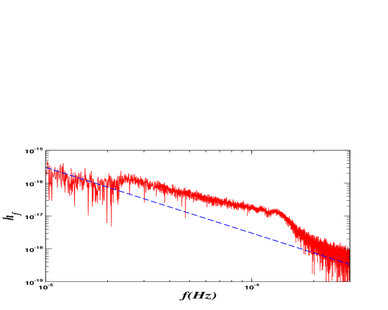
where $L=5\times 10^{6}$ kms is the arm-length for LISA, $S_{n}^{pos}=4\times 10^{-22}\,m^{2}/Hz$ and $S_{n}^{accel}=9\times 10^{-30}\,m^{2}/s^{4}/Hz$ are the position and acceleration noise respectively. Using this formula, we generate instrumental noise from a Gaussian distribution. In Figure 1 we display the power spectrum of the LISA response to the system we are investigating with instrumental noise from one channel of LISA. Our analysis uses LISA as a two channel detector, where the detectors are rotated by a factor of $\pi/2$ with respect to one another [10]. We also assume that LISA has a lower frequency cutoff of $10^{-5}$ Hz.

Figure 1: A plot of the strain spectral density of the LISA response to a $10^{7}-10^{6}\,M_{\odot}$ binary at $z=1$. The dashed line indicates the RMS instrument noise level.

3 The MCMC approach

In the Bayesian framework of data analysis, the goal is to calculate the posterior probability density functions for the parameters of the model, given the parameter priors and the data. However, this is extremely difficult, if not impossible, to do analytically. The advantage of the MCMC method is that it allows one to map out the posterior numerically. Our MCMC approach is implemented by using a Metropolis-Hastings algorithm to map out the posterior distributions of the 9-D parameter space for Super Massive black holes. The method works as follows: We assume that we have already run a search chain that has found the system we are looking for. We use the true parameter values as the starting point for our chain $\vec{x}$. The algorithm then suggests a jump to a new point $\vec{y}$ using a proposal distribution $q(^{.}|\vec{x})$. We evaluate the Hastings ratio

$$H=\frac{\pi(\vec{y})p(s|\vec{y})q(\vec{x}|\vec{y})}{\pi(\vec{x})p(s|\vec{x})q(\vec{y}|\vec{x})},$$ (2)

and accept the jump with probability $\alpha={\rm min}(1,H)$, otherwise the chain stays at its current position. Here $\pi(\vec{x})$ are the priors of the parameters and $p(s|\vec{x})$ is the likelihood. We use uniform priors for all the parameters. The parameters $\ln M_{c}$, $\ln\mu$, $\ln t_{c}$ and $\ln D_{L}$ were taken to be uniform in the range $(-\infty,\infty)$, $\cos\theta$ and $\cos\iota$ were taken to be uniform in the range $[-1,1]$, $\phi$ and $\varphi_{c}$ were taken to be uniform in the range $[0,2\pi]$, and $\psi$ was taken to be uniform in the range $[0,\pi]$. The log-likelihood for a template $h(\vec{x})$ given a signal $s$ was assumed to have the form

$$\ln p\left(s|\vec{x}\right)=-\frac{1}{2}\langle s-h(\vec{x})|s-h(\vec{x})\rangle.$$ (3)

Here the angular brackets define the standard noise weighted inner product. In order to achieve a healthy acceptance rate for the proposed jumps, we use a proposal distribution given by a multivariate normal distribution that is the product of independent normal distributions in each of the 9 eigendirection of the Fisher matrix, $\Gamma_{ij}(\vec{x})$. The Fisher information matrix describes the expectation value of the curvature of the log likelihood function at maximum likelihood:

$$\Gamma_{ij}(\vec{x}_{\rm ML})=\overline{\partial_{i}\partial_{j}\ln p\left(s|\vec{x}_{\rm ML}\right)}=\langle\partial_{i}h(\vec{x}_{\rm ML})|\partial_{j}h(\vec{x}_{\rm ML})\rangle\,.$$ (4)

Here the over line indicates the expectation value. We used a generalized notion of the Fisher matrix by employing the definition $\Gamma_{ij}(\vec{x})=\langle\partial_{i}h(\vec{x})|\partial_{j}h(\vec{x})\rangle$ for points $\vec{x}$ away from maximum likelihood. The standard deviation in each eigendirection of $\Gamma_{ij}(\vec{x})$ was set to equal $\sigma_{i}=1/\sqrt{DE_{i}(\vec{x})}$, where $D=9$ and $E_{i}(\vec{x})$ is the corresponding eigenvalue. The factor of $1/\sqrt{D}$ ensures that the typical jumps are $\sim 1\sigma$ for the full multivariate normal distribution. In principle this choice of proposal distribution should yield a $\sim 69\%$ acceptance rate for the proposed jumps. In practice we found an acceptance rate of $\sim 33\%$ for the system being studied. The lower acceptance rate is due to the Fisher matrix slightly overestimating the uncertainties in one of the eigendirections, and to a slight error in the estimate of the orientation of the corresponding eigendirection.

4 Results

Figure 2: A plot of the MCMC chains for the 9 parameters describing the SMBHB binary during the initial burn-in phase. The straight line in each panel denotes the true parameter value.

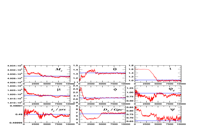
We started the chain with parameter values close to their true values, but offset by $\Delta m_{1}/m_{1}=-0.2\%$, $\Delta m_{2}/m_{2}=+0.3\%$, $\Delta z=+0.2$, $\Delta t_{c}/t_{c}=-2\times 10^{-5}$, $\Delta\theta=-0.2$, $\Delta\phi=+0.2$, $\Delta\iota=+0.6$, $\Delta\psi=+0.2$, and $\Delta\phi_{c}=-0.4$. The offset in each parameter was chosen to be $\sim$tens of standard deviations away from the true source parameters (as estimated by the Fisher Information Matrix). In Figure 2 we see that the chain underwent a burn-in phase during the first 10,000 steps, before settling in close to the true source parameters. In repeated trials we found that the chain always settled in to the same region of parameter space after the burn-in was completed. When the chain was started off far from the true parameters the burn-in time became prohibitively long, so we do not recommend that the current algorithm be used for blind searches. We have developed a non-Markovian variant of the algorithm that can efficiently handle the search phase [18]. The posterior distribution functions derived after the full search are identical to those found in the current paper.

Figure 3: A plot of the MCMC chains for the 9 parameters describing the SMBHB binary. The straight line in each panel denotes the mean of the chain as calculated from the $8\times 10^{6}$ points. The dashed lines are the $2-\sigma$ predictions from the Fisher matrix evaluated at the mean of each chain.

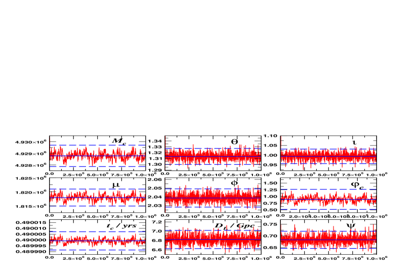
Following the burn-in, the chain was run for another $8\times 10^{6}$ points to explore the posterior distribution function. This took 8 days on a single 2 GHz processor. The first million points of the exploration phase of the chain are shown in Figure 3. We see that the MCMC chain moves around well, and show clear evidence of the high degree of correlation between the parameters $M_{c},\mu,t_{c}$ and $\varphi_{c}$. The straight, solid line in each panel of Figure 3 denotes the mean value of the parameter, as calculated from the chain. Taking this mean value, we then calculated the standard deviation as predicted by the Fisher matrix at that point. This $1-\sigma$ error is given by

$$\sigma_{i}=\sqrt{C_{ii}},$$ (5)

where $C_{ij}=(\Gamma_{ij})^{-1}$. The two dashed lines in each panel denote the $\pm 2\sigma$ errors in each of the parameters.

Figure 4: A plot of the marginalized 1-d histograms for each of the nine parameters. We see that most of the angular variables agree almost exactly with the prediction of the Fisher matrix. However, the remaining four parameters, which are all highly correlated, differ from the Fisher matrix prediction for the posterior.

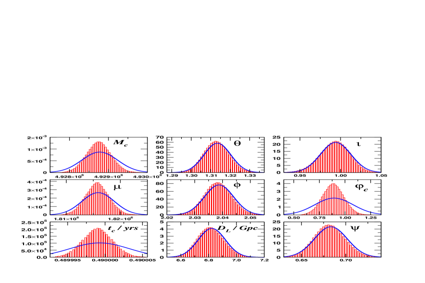
In Figure 4 we have plotted the 1-D marginalized histograms for each of the parameters. The solid line is the Fisher matrix prediction for the error at the mean of each chain. We can see that most of the extrinsic parameter histograms match the Fisher prediction almost perfectly. This is also the case for the $(\theta,\phi)$ parameters. However, we can see that the histograms for $(M_{c},\mu,t_{c},\varphi_{c})$ all differ from the prediction of the Fisher matrix. We attribute the error in the Fisher matrix prediction to the high degree of correlation between these parameters. In order to see just how correlated these parameters are, in Figure 5 we plot the 2-D marginalized histograms for the combinations $(M_{c},\varphi_{c})$, $(\mu,\varphi_{c})$, $(t_{c},\varphi_{c})$, and $(M_{c},\mu)$. We found that the Fisher matrix has a small eigenvalue in the $(M_{c},\mu,t_{c},\varphi_{c})$ direction which dominates the contribution to the proposed jumps in these parameters. The Fisher matrix tends to under estimate the eigenvalue in this direction, and it is also slightly off in predicting the corresponding eigendirection. Similar behavior was seen in all the examples we have looked at, which suggests that the Fisher matrix estimates for the uncertainties in the component masses found in the literature may be systematically high by about a factor of two.

    

    

Figure 5: This figure showing the 2-D marginalized histograms demonstrates the large correlations between the parameters $(M_{c},\mu,t_{c},\varphi_{c})$.

In a closely related study that appears in these same proceedings, Wickham, Stroeer & Vecchio [19] use a Reversible Jump MCMC routine to study the posterior parameter distributions of a SMBHB system. They used a simplified model of the SMBHB waveform, which removes the reduced mass from the parameter set. In contrast to our findings, they found that the Fisher matrix significantly underestimated the uncertainties in many of the model parameters. We do not know why our results are so different, but we do not think it is due to the differences in our MCMC implementations. The Reverse Jump method should yield the same results as our standard MCMC implementation when applied to models with fixed numbers of parameters.

5 Discussion

We have found that it is possible to construct a simple MCMC sampler for studying the posterior distribution functions for SMBHB inspirals in the LISA data streams. The marginalized posterior distributions recovered from the Markov chains are in good to fair agreement with the Fisher matrix predictions. In another work [18], we have developed an advanced MCMC search routine that is capable of performing a blind search of the LISA data for SMBHB inspirals.

References

- [1] P. Bender et al., LISA pre-phase A report (1998)
- [2] E. Berti, V. Cardoso & C. M. Will, Phys. Rev. D73, 064030 (2006).
- [3] J. R. Gair, L. Barack, T. Creighton, C. Cutler, S. L. Larson, E. S. Phinney & M. Vallisneri, Class. Quant. Grav. 21, S1595 (2004).
- [4] N.J. Cornish & S.L. Larson, Phys. Rev. D67, 103001 (2003).
- [5] N.J. Cornish & J. Crowder, Phys. Rev. D72, 043005 (2005).
- [6] J. Crowder, N.J. Cornish & L. Reddinger, Phys. Rev. D73, 063011 (2006).
- [7] S. D. Mohanty & R. K. Nayak, Phys. Rev. D73, 083006 (2006).
- [8] N. Christensen, R. J. Dupuis, G. Woan & R. Meyer, Phys. Rev. D70, 022001 (2004); R. Umstatter, R. Meyer, R. J. Dupuis, J. Veitch, G. Woan & N. Christensen, AIP Conf. Proc. 735 (2005); N. Christensen, A. Libson & R. Meyer, Class. Quant. Grav. 21 317 (2004); C. Rover, R. Meyer & N. Christensen, gr-qc/0602067 (2006).
- [9] R. Umstatter, N. Christensen, M. Hendry, R. Meyer, V. Simha, J. Veitch & S. Vigeland, G. Woan, Phys. Rev. D72, 022001 (2005)
- [10] C. Cutler, Phys. Rev. D57, 7089 (1998).
- [11] T. A. Moore & R. W. Hellings, Phys. Rev. D65, 062001 (2002).
- [12] S. A. Hughes, Mon. Not. Roy. Astron. Soc. 331 805 (2002).
- [13] N. Seto, Phys. Rev. D66, 122001 (2002).
- [14] A. Vecchio, Phys. Rev. D67, 022001 (2003).
- [15] L. Blanchet, B. R. Iyer, C. M. Will and A. G. Wiseman, Class. Quant. Grav. 13, 575 (1996).
- [16] N. J. Cornish & L. J. Rubbo, Phys. Rev. D67, 022001 (2003).
- [17] B. J. Owen, Phys. Rev. D53, 6749 (1996).
- [18] N. J. Cornish & E. K. Porter, preprint gr-qc/0605135 (2006).
- [19] E. D. L. Wickham, A. Stroeer & A. Vecchio, preprint gr-qc/0605071 (2006).