Gravitational radiation from nonaxisymmetric spherical Couette flow in a neutron star

Abstract

The gravitational wave signal generated by global, nonaxisymmetric shear flows in a neutron star is calculated numerically by integrating the incompressible Navier–Stokes equation in a spherical, differentially rotating shell. At Reynolds numbers ${\it Re}\lower 2.15277pt\hbox{$\;\buildrel>\over{\sim}\;$}3\times 10^{3}$, the laminar Stokes flow is unstable and helical, oscillating Taylor–Görtler vortices develop. The gravitational wave strain generated by the resulting kinetic-energy fluctuations is computed in both $+$ and $\times$ polarizations as a function of time. It is found that the signal-to-noise ratio for a coherent, $10^{8}$-s integration with LIGO II scales as $6.5(\Omega_{*}/10^{4}\,{\rm rad}\,{\rm s}^{-1})^{7/2}$ for a star at $1$ kpc with angular velocity $\Omega_{*}$. This should be regarded as a lower limit: it excludes pressure fluctuations, herringbone flows, Stuart vortices, and fully developed turbulence (for ${\it Re}\lower 2.15277pt\hbox{$\;\buildrel>\over{\sim}\;$}10^{6}$).

1 Introduction

Gravitational radiation from linear, global, fluid oscillations in neutron stars has been studied extensively, e.g. radiation-reaction-driven r-modes (Andersson, 1998; Levin & Ushomirsky, 2001), and two-stream superfluid oscillations with entrainment (Andersson, 2003; Prix et al., 2004). However, gravitational radiation is also emitted by nonlinear, global, fluid oscillations. Specifically, it is well known that a viscous Navier–Stokes fluid inside a spherical, differentially rotating shell — spherical Couette flow (SCF) — undergoes sudden transitions between states with different vortex topologies, which are generally nonaxisymmetric, due to shear instabilities (Marcus & Tuckerman, 1987a, b; Junk & Egbers, 2000). Recent simulations of superfluid SCF, based on the Hall–Vinen–Bekarevich–Khalatnikov (HVBK) theory of a ${}^{1}S_{0}$ neutron superfluid, confirm that such transitions to nonaxisymmetric flows also occur in neutron stars (Peralta et al., 2005, 2006).

In this Letter, we compute the gravitational wave signal generated by nonaxisymmetric flows in young, rapidly rotating neutron stars. There are at least two astrophysical scenarios in which these develop. First, if the crust and core of the star are loosely coupled, as indicated by observations of pulsar glitches (Shemar & Lyne, 1996; Lyne et al., 2000), differential rotation builds up as the crust spins down electromagnetically, until the core undergoes a transition to the Taylor–Görtler vortex state, a helical, oscillating flow that is one of the last stages in the laminar-turbulent transition in SCF as the Reynolds number increases (Nakabayashi, 1983; Nakabayashi & Tsuchida, 1988). Second, if the crust precesses, while the core does not, the rotation axes of the crust and core misalign, inducing a rich variety of flow patterns and instabilities, like time-dependent shear waves, leading to fully developed turbulence (Wilde & Vanyo, 1995). We treat the former scenario here and postpone the latter to a separate paper.

In §2, an SCF model of a differentially rotating neutron star is proposed. In §3, we explore the transitional dynamics and topology of the flow. In §4, we calculate the gravitational wave signal and its frequency spectrum.

2 Global SCF model and numerical method

We consider an idealized, two-component model of a neutron star, in which a solid crust is loosely coupled to a differentially rotating fluid core. Specifically, we consider the motion of a neutron fluid within a spherical, differentially rotating shell in the outer core of the star, where the density $\rho$ lies in the range $0.6<\rho/\rho_{c}<1.5$, $\rho_{c}=2.6\times 10^{14}\,{\rm g\,cm}^{-3}$ (Sedrakian & Sedrakian, 1995). The inner (radius $R_{1}$) and outer (radius $R_{2}$) boundaries rotate at angular frequencies $\Omega_{1}$ and $\Omega_{2}$, respectively, about the $z$ axis. As the star is strongly stratified, the shell is thin, with $R_{2}-R_{1}\leq 0.1R_{1}$ (Abney & Epstein, 1996; Levin & D’Angelo, 2004). The rotational shear is sustained by the vacuum-dipole spin-down torque, violent events at birth (Dimmelmeier et al., 2002; Ott et al., 2004), accretion in a binary (Fujimoto, 1993), neutron star mergers (Shibata & Uryū, 2000), or internal oscillations like r-modes (Rezzolla et al., 2000; Levin & Ushomirsky, 2001).

We describe the fluid by the isothermal Navier–Stokes equation, which, in the inertial frame of an external observer, takes the form

$$\frac{\partial{\bf v}}{\partial t}+({\bf v}\!\cdot\!\nabla){\bf v}=-\frac{\nabla p}{\rho}+\nu\nabla^{2}{\bf v}+\nabla\Phi$$ (1)

in the incompressible limit $\nabla\cdot{\bf v}=0$, where ${\bf v}$ is the fluid velocity, $\nu$ is the kinematic viscosity, $\rho$ is the density, $p$ is the pressure, and $\Phi$ is the Newtonian gravitational potential. Henceforth, $\Phi$ is absorbed into $p$ by replacing $p-\rho\Phi$ with $p$, such that pressure balances gravity in the stationary equilibrium (${\bf v}=0$) and there are no gravitational forces driving the flow in the incompressible limit when the stationary equilibrium is perturbed. The Reynolds number and dimensionless gap width are defined by ${\it Re}=\Omega_{1}R_{1}^{2}/\nu$ and $\delta=(R_{2}-R_{1})/R_{1}$; the rotational shear is $\Delta\Omega=\Omega_{2}-\Omega_{1}$. Equation (1) is solved subject to no-slip boundary conditions.

Superfluidity plays a central role in the thermal (Yakovlev et al., 1999) and hydrodynamic (Alpar, 1978; Reisenegger, 1993; Peralta et al., 2005) behavior of neutron star interiors. However, we assume a viscous fluid here. Counterintuitively, this is a good approximation because ${\it Re}$ ($\sim 10^{11}$) is very high (Mastrano & Melatos, 2005). It is known from terrestrial experiments on superfluid ⁴He that, at high ${\it Re}$, quantized vortices tend to lock the superfluid to turbulent eddies in the normal fluid by mutual friction (Barenghi et al., 1997), so that the superfluid resembles classical Navier–Stokes turbulence. Moreover, in HVBK simulations of SCF, it is observed that the global circulation pattern of the superfluid does not differ much from a Navier–Stokes fluid at ${\it Re}\lower 2.15277pt\hbox{$\;\buildrel>\over{\sim}\;$}250$ (Henderson & Barenghi, 2004; Peralta et al., 2005). Finally, a viscous interior is expected in newly born neutron stars, which are hotter than the superfluidity transition temperature (Andersson et al., 1999).

By assuming a viscous fluid, we omit from (1) the coupling between quantized vortices and the normal fluid (Hall & Vinen, 1956), entrainment of superfluid neutrons by protons (Comer, 2002), and pinning of quantized vortices in the inner crust, at radius $R_{1}$ [Baym et al. (1992); cf. Jones (1998)]. We also neglect vortex pinning in the outer core for simplicity, even though evidence exists that it may be important when magnetic fields are included. Specifically, three-fluid models of post-glitch relaxation based on the core dynamics favor vortex pinning at the phase separation boundary of the core (Sedrakian & Sedrakian, 1995), e.g. due to the interaction between vortex clusters and the Meissner supercurrent set up by the crustal magnetic field at the phase boundary (Sedrakian & Cordes, 1999). Other models analyze interpinning of proton and neutron vortices in the core (Ruderman, 1991) and its effect on precession (Link, 2003). In the context of the hydrodynamic model in this paper, pinning effectively increases the viscosity of the core, reducing ${\it Re}$.

We use a pseudospectral collocation method to solve equation (1) (Bagchi & Balachandar, 2002; Giacobello, 2005). The equations are spatially discretized in spherical polar coordinates $(r,\theta,\phi)$, using restricted Fourier expansions in $\theta$ and $\phi$ and a Chebyshev expansion in $r$. The solution is advanced using a two-step fractional-step method, which is accurate to second order in the time-step (Canuto et al., 1988). We limit ourselves to narrow gaps $\delta\leq 0.1$, which are computationally less expensive and for which more experimental studies are available for comparison (Yavorskaya et al., 1977; Nakabayashi, 1983). Recently, we performed the first stable simulations of superfluid SCF using this method (Peralta et al., 2005).

3 Nonaxisymmetric spherical Couette flow

The bifurcations and instabilities leading to transitions between SCF states are controlled by three parameters: $\delta$, ${\it Re}$, and $\Delta\Omega$. Additionally, the history of the flow influences its post-instability evolution and the final transition to turbulence (Wulf et al., 1999; Junk & Egbers, 2000). For example, in experiments on Taylor-Görtler vortices (TGV), the final state depends on $d\Omega_{1}/dt$, i.e. on the time to reach the critical ${\it Re}$ relative to the viscous diffusion time (Nakabayashi & Tsuchida, 1995). In general, four SCF states can be distinguished: (i) a laminar basic flow, (ii) a toroidal or helical Taylor–Görtler flow, (iii) a transitional flow with nonaxisymmetric, oscillating TGV, and (iv) fully developed turbulence (Yavorskaya et al., 1975; Nakabayashi, 1983). In a neutron star, where ${\it Re}\sim 10^{11}$, the state is probably turbulent. However, we are restricted by our computational resources to simulate regimes (i) and (ii), with $1\times 10^{3}\leq{\it Re}\leq 3\times 10^{4}$.

3.1 TGV transition: initial conditions

Experimentally, for $\delta=0.06$, TGV are obtained by quasistatically increasing $\Omega_{1}$ from zero to give ${\it Re}\sim 3300$ (Nakabayashi & Tsuchida, 2005). This procedure can be painfully slow, because a steady state must be reached at each intermediate step. Numerically, we circumvent it by following Li (2004) and introducing a nonaxisymmetric perturbation with azimuthal wave number $m_{a}$ of the form

$$v_{r} = -\frac{4\epsilon_{1}(r-R_{1})(r-R_{2})}{\delta^{2}R_{1}^{2}}\cos\chi(\theta,\phi),$$ (2)

$$v_{\theta} = \frac{\epsilon_{1}}{\delta}\sin\left[\frac{\pi(r-R_{1})(r-R_{2})}{2(R_{2}-R_{1})^{2}}\right]\sin\chi(\theta,\phi),$$ (3)

with $\chi=\pi[1-R_{2}(\pi/2-\theta)/(R_{2}-R_{1})-0.4\sin(m_{a}\phi)]$. This is done as follows. Before introducing the perturbation, a steady state for ${\it Re}=2667$ is obtained (just below the critical ${\it Re}$ where TGV emerge experimentally). Then, the Reynolds number is raised instantaneously to ${\it Re}=3300$, and we continue by adding (2) and (3), with amplitude $\epsilon_{1}\sim 10^{-6}\,\Omega_{1}R_{1}$, to the numerical solution at each time-step until a viscous diffusion time $t_{d}=(R_{2}-R_{1})^{2}/\nu$ elapses. We then stop adding the perturbation and the flow is left to evolve according to (1), until a final steady state is reached. More than one perturbation can lead to the same final state; some authors add Gaussian noise (Zikanov, 1996), although this affords less control over the wavenumber and the number of vortices excited.

The perturbation excites TGV by shedding vorticity from the inner sphere (Li, 2004). Perturbations with $2\leq m_{a}\leq 5$ are explored, supplementing experiments with $m_{a}=3$ (Nakabayashi, 1983). For numerical simplicity, we limit ourselves to the case where only the inner sphere rotates. TGV with both spheres rotating are equally possible and have been observed experimentally; they exhibit additional twisting (and increased nonaxisymmetry) in the helical vortices (Nakabayashi & Tsuchida, 2005), so the gravitational wave strain we compute in §4 is a lower limit.

3.2 Flow topology

Figure 1a shows a kinetic-energy-density isosurface $(0.11\rho R_{1}^{5}\Omega_{1}^{2})$ for the fully developed TGV state $m_{a}=3$, $\delta=0.06$, ${\it Re}=3300$. Its nonaxisymmetry is apparent in the striated equatorial bands, whose inclination with respect to the equator varies with longitude from zero to $\sim 3$ deg (Nakabayashi, 1983).

A popular way to classify complex, three-dimensional flows is to construct scalar invariants from $A_{ij}=\partial v_{i}/\partial x_{j}$ (Chong et al., 1990; Jeong & Hussain, 1995). Specifically, the discriminant $D_{A}=Q_{A}^{3}+27R_{A}^{2}/4$, with $R_{A}=-{\rm det}(A_{ij})$ and $Q_{A}=(A_{ii}^{2}-A_{ij}A_{ji})/2$, distinguishes between regions which are focal ($D_{A}>0$) and strain-dominated ($D_{A}<0$). Figure 1b plots the $D_{A}=10^{-3}\,\Omega_{1}^{6}$ isosurface in color: yellow regions are stable focus/stretching, blue regions are unstable focus/contracting. The filaments coincide with the TGV. One circumferential vortex and $m_{a}=3$ helical vortices lie in each hemisphere. We also plot the isosurface $D_{A}=-10^{-3}\,\Omega_{1}^{6}$: red and green regions have stable node/saddle/saddle and unstable node/saddle/saddle topologies respectively (Chong et al., 1990). The helical vortices span $\sim 40$ deg of latitude and travel in the $\phi$ direction, with phase speed $\approx 0.48\Omega_{1}R_{1}$.

The TGV state is oscillatory, which is important for the gravitational wave spectrum. Its periodicity is evident in Figure 1c, where $v_{\theta}$ at an equatorial point is plotted versus time for $2\leq m_{a}\leq 5$. For $m_{a}=3$, $v_{\theta}$ oscillates with period $4.4\Omega_{1}^{-1}$, the time for successive helical vortices to pass by a stationary observer, in accord with experiments (Nakabayashi, 1983). Instantaneous streamlines are drawn in three meridional planes in Figure 1d, highlighting the nonaxisymmetry. One obtains a similar TGV state for $\delta=0.14$, $=0.18$ (Sha & Nakabayashi, 2001; Li, 2004).

4 Gravitational wave signal

The metric perturbation $h_{ij}^{\rm TT}=(4G/rc^{4})\int d^{3}{\bf x}\,T_{ij}$ in the transverse-traceless gauge can be calculated using Einstein’s quadrupole formula (Misner et al., 1973)

$$h_{ij}^{\rm TT}=\frac{2G\rho}{rc^{6}}\frac{\partial^{2}}{\partial t^{2}}\int d^{3}{\bf x}\,|{\bf v}|^{2}\left(x_{i}x_{j}-\delta_{ij}\frac{|{\bf x}|^{2}}{3}\right),$$ (4)

where the integral is over the source volume, $r$ is the distance to the source, and $T_{ij}=\rho\gamma^{2}v_{i}v_{j}+p\delta_{ij}$ is the stress-energy of a Newtonian fluid. Note that we approximate $T_{00}=\rho\gamma^{2}\approx\rho(1+|{\bf v}|^{2}/c^{2})$ in (4), and we omit a thermal-energy contribution $\propto\delta p$ ($\sim\rho|{\bf v}|^{2}$, by Bernoulli’s theorem), which we cannot calculate with our incompressible solver. Far from the source, we write $h^{\rm TT}_{ij}=h_{+}e_{ij}^{+}+h_{\times}e_{ij}^{\times}$, with the polarizations defined by $e_{yy}^{+}=-e_{zz}^{+}=e^{\times}_{yz}=e^{\times}_{zy}=1$ for an observer on the $x$ axis.

In Figure 2a, we plot the $h_{+}$ and $h_{\times}$ polarizations versus time, as seen by an observer on the $x$ axis, for $2\leq m_{a}\leq 5$ (the signal is $\sim 3$ times weaker on the $z$ axis, where the north-south asymmetry is not seen in projection). The amplitude is greatest for $m_{a}=5$ but depends weakly on $m_{a}$. Importantly, $h_{+}$ and $h_{\times}$ are $\pi/2$ out of phase for all $m_{a}$, and we find $|h_{+}|\ll|h_{\times}|$ for even $m_{a}$. These two signatures offer a promising target for future observations. The period ($\approx 0.8\Omega_{1}^{-1}$) is similar for $3\leq m_{a}\leq 5$, where a maximum of three helical vortices are excited (Li, 2004) (we find that the torque at $R_{2}$ oscillates with the same period). This too is good for detection, because several modes are likely to be excited in a real star. The period arises because the isosurface in Figure 1a forms a pattern with six-fold symmetry when projected onto the $y$-$z$ plane, with fundamental period $4.4\Omega_{1}^{-1}$

In Figure 2b, we present the frequency spectra of the $+$ and $\times$ polarizations. The two peaks, at $f\approx 1.2\Omega_{1}$ and $2.4\Omega_{1}$, have full-width-half-maxima of $\sim 300$ Hz. This is caused by the subharmonics evident in Figure 1c, which arise because the northern and southern helical vortices start at unequal and variable longitudes. In addition, the peaks for even and odd $m_{a}$ are displaced by $\sim 500$ Hz, and the primary peak for $m_{a}=4$ is split. These two spectral signatures are a promising target for future observations. The even-odd displacement may arise because the phase speeds of the vortex patterns for $m_{a}=2$, $3$ differ by $\approx 0.01\Omega_{1}R_{1}$ (Li, 2004). For large $f$, we find $h_{+,\times}(f)\propto f^{-3/2}$.

The squared signal-to-noise ratio can be calculated from $(S/N)^{2}=4\int_{0}^{\infty}df|h(f)|^{2}/S_{h}(f)$ (Creighton, 2003), where we take $S_{h}(f)=10^{-50}(f/0.6\,{\rm kHz})^{2}$ ($0.2\leq f\leq 3$ kHz) for a $10^{8}$-s integration with LIGO II, if the frequency and phase of the signal are known in advance (Brady et al., 1998). For a star with $\Omega_{1}/2\pi=600$ Hz, at $r=1$ kpc, we find $S/N=0.21$ ($m_{a}=2$), $0.12$ ($m_{a}=3$), $0.023$ ($m_{a}=4$), and $0.22$ ($m_{a}=5$), although there will be some leakage of signal when the coherent integration is performed, because the spectrum is not monochromatic. For $m_{a}\leq 5$, $S/N$ increases (decreases) as $m_{a}$ odd (even) increases. We also find $S/N\propto\Omega_{1}^{7/2}$, which implies that the fastest millisecond pulsars ($\Omega_{1}/2\pi\sim 1$ kHz) and newly born pulsars with $\Delta\Omega/\Omega_{1}\sim 0.1$ are most likely to be detected. The flow states leading to turbulence at ${\it Re}\lower 2.15277pt\hbox{$\;\buildrel>\over{\sim}\;$}10^{6}$, e.g. shear waves, Stuart vortices, and “herringbone” waves (Nakabayashi & Tsuchida, 1988), make contributions of similar order to the TGV signal in Figure 2.

The Reynolds number in the outer core of a neutron star, ${\it Re}=10^{10}(\rho/10^{15}\,{\rm g}\,{\rm cm}^{-3})^{-1}$ $(T/10^{8}\,{\rm K})^{2}(\Omega_{*}/10^{4}\,{\rm rad}\,{\rm s}^{-1})$ (Mastrano & Melatos, 2005), where $T$ is the temperature, typically exceeds the maximum ${\it Re}$ in our simulations (due to computational capacity). For ${\it Re}\lower 2.15277pt\hbox{$\;\buildrel>\over{\sim}\;$}10^{6}$, the flow is turbulent and therefore axisymmetric when time-averaged — but not instantaneously. In Kolmogorov turbulence, the characteristic flow speed in an eddy of wavenumber $k$ scales as $k^{-1/3}$, the turbulent kinetic energy scales as $k^{-5/3}$, and the turn-over time scales as $k^{-2/3}$. From equation (4), the rms wave strain scales as $k^{-3/2}\int dk\,k^{-1/3}$ after averaging over Gaussian fluctuations, and is dominated by the largest eddies (where most of the kinetic energy also resides). We therefore conclude that, even for ${\it Re}\lower 2.15277pt\hbox{$\;\buildrel>\over{\sim}\;$}10^{6}$, the largest eddies, which resemble organized structures like TGV, dominate $h_{+}$ and $h_{\times}$, not the isotropic small eddies, but the signal is noisier. Hence, counterintuitively, we predict that hotter neutron stars (with lower ${\it Re}$) have narrower gravitational wave spectra than cooler neutron stars, ceteris paribus.

We ignore compressibility when computing $T_{00}$ ($\delta p=0$) and solving (1) numerically by pressure projection. Yet, realistically, neutron stars are strongly stratified (Abney & Epstein, 1996), confining the meridional flow in Figure 1d into narrow layers near $r=R_{1}$, $R_{2}$. Stratification can be implemented crudely by using a low-pass spectral filter to artificially suppres $v_{r}$ (Don, 1994; Peralta et al., 2006). We postpone this to future work.

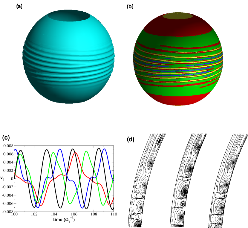
Figure 1: Taylor-Görtler vortices for $m_{a}=3$, $\delta=0.06$, at $t=100\,\Omega_{1}^{-1}$. (a) Isosurface of kinetic energy: $\rho|{\bf v}|^{2}=0.11\rho R_{1}^{5}\Omega_{1}^{2}$. (b) Isosurfaces of velocity-gradient discriminant: $D_{A}=10^{-3}\,\Omega_{1}^{6}$, stable focus/stretching (yellow) and unstable focus/contracting (blue); $D_{A}=-10^{-3}\,\Omega_{1}^{6}$, stable node/saddle/saddle (red) and unstable node/saddle/saddle (green). (c) Time history of $v_{\theta}$ at $r=1.06$, $\theta=\pi/2$, $\phi=0$ for $m_{a}=2$ (red), $3$ (blue), $4$ (green), and $5$ (black). (d) Streamlines obtained by integrating the in-plane components of ${\bf v}$ in the planes $\phi=0$ (left), $\phi=\pi/2$ (middle), and $\phi=2\pi/9$ (right).

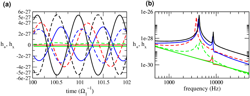
Figure 2: Gravitational waves from Taylor-Görtler vortices in a neutron star with $\Omega_{1}/2\pi=600$ Hz and $r=1$ kpc. (a) Signal $h_{+,\times}(t)$, and (b) frequency spectrum $h_{+,\times}(f)$, for $m_{a}=2$ (red), $3$ (blue), $4$ (green), and $5$ (black). Solid and dashed curves correspond to the $+$ and $\times$ polarizations respectively, as measured by an observer on the $x$ axis.

References

- Abney & Epstein (1996) Abney, M., & Epstein, R. I. 1996, J. Fluid Mech., 312, 327
- Alpar (1978) Alpar, M. A. 1978, J. Low Temp. Phys., 31, 803
- Andersson (1998) Andersson, N. 1998, ApJ, 502, 708
- Andersson (2003) —. 2003, Classical Quant. Grav., 20, 105
- Andersson et al. (1999) Andersson, N., Kokkotas, K., & Schutz, B. F. 1999, ApJ, 510, 846
- Bagchi & Balachandar (2002) Bagchi, B., & Balachandar, S. 2002, J. Fluid. Mech., 466, 365
- Barenghi et al. (1997) Barenghi, C. F., Samuels, D. C., Bauer, G. H., & Donnelly, R. J. 1997, Phys. Fluids, 9, 2631
- Baym et al. (1992) Baym, G., Epstein, R., & Link, B. 1992, Physica B, 178, 1
- Brady et al. (1998) Brady, P. R., Creighton, T., Cutler, C., & Schutz, B. F. 1998, Phys. Rev. D, 57, 2101
- Canuto et al. (1988) Canuto, C., Hussaini, M., Quarteroni, A., & Zang, T. 1988, Spectral Methods in Fluid Dynamics (Springer-Verlag)
- Chong et al. (1990) Chong, M. S., Perry, A. E., & Cantwell, B. J. 1990, Phys. Fluids, 2, 765
- Comer (2002) Comer, G. L. 2002, Found. Phys., 32, 1903
- Creighton (2003) Creighton, T. 2003, Classical Quant. Grav., 20, 853
- Dimmelmeier et al. (2002) Dimmelmeier, H., Font, J. A., & Müller, E. 2002, A&A, 393, 523
- Don (1994) Don, W. S. 1994, J. Comput. Phys., 110, 103
- Fujimoto (1993) Fujimoto, M. Y. 1993, ApJ, 419, 768
- Giacobello (2005) Giacobello, M. 2005, PhD thesis, University of Melbourne
- Hall & Vinen (1956) Hall, H. E., & Vinen, W. F. 1956, Proc. R. Soc. Lond., A238, 204
- Henderson & Barenghi (2004) Henderson, K. L., & Barenghi, C. F. 2004, Theor. Comp. Fluid Dyn., 18, 183
- Jeong & Hussain (1995) Jeong, J., & Hussain, F. 1995, J. Fluid Mech., 285, 69
- Jones (1998) Jones, P. B. 1998, MNRAS, 296, 217
- Junk & Egbers (2000) Junk, M., & Egbers, C. 2000, LNP Vol. 549: Physics of Rotating Fluids, 549, 215
- Levin & D’Angelo (2004) Levin, Y., & D’Angelo, C. 2004, ApJ, 613, 1157
- Levin & Ushomirsky (2001) Levin, Y., & Ushomirsky, G. 2001, MNRAS, 324, 917
- Li (2004) Li, Y. 2004, Sci. China Ser. A, 47, 81
- Link (2003) Link, B. 2003, Phys. Rev. Lett., 91, 101101
- Lyne et al. (2000) Lyne, A. G., Shemar, S. L., & Smith, F. G. 2000, MNRAS, 315, 534
- Marcus & Tuckerman (1987a) Marcus, P., & Tuckerman, L. 1987a, J. Fluid Mech., 185, 1
- Marcus & Tuckerman (1987b) —. 1987b, J. Fluid Mech., 185, 31
- Mastrano & Melatos (2005) Mastrano, A., & Melatos, A. 2005, MNRAS, 361, 927
- Misner et al. (1973) Misner, C. W., Thorne, K. S., & Wheeler, J. A. 1973, Gravitation (San Francisco: W.H. Freeman and Co., 1973)
- Nakabayashi (1983) Nakabayashi, K. 1983, J. Fluid Mech., 132, 209
- Nakabayashi & Tsuchida (1988) Nakabayashi, K., & Tsuchida, Y. 1988, J. Fluid Mech., 194, 101
- Nakabayashi & Tsuchida (1995) —. 1995, J. Fluid Mech., 295, 43
- Nakabayashi & Tsuchida (2005) —. 2005, Phys. Fluids, 17, 4110
- Ott et al. (2004) Ott, C. D., Burrows, A., Livne, E., & Walder, R. 2004, ApJ, 600, 834
- Peralta et al. (2005) Peralta, C., Melatos, A., Giacobello, M., & Ooi, A. 2005, ApJ, 635, 1224
- Peralta et al. (2006) —. 2006, Submitted to ApJ
- Prix et al. (2004) Prix, R., Comer, G. L., & Andersson, N. 2004, MNRAS, 348, 625
- Reisenegger (1993) Reisenegger, A. 1993, J. Low Temp. Phys., 92, 77
- Rezzolla et al. (2000) Rezzolla, L., Lamb, F. K., & Shapiro, S. L. 2000, ApJ, 531, L139
- Ruderman (1991) Ruderman, M. 1991, ApJ, 382, 587
- Sedrakian & Cordes (1999) Sedrakian, A., & Cordes, J. M. 1999, MNRAS, 307, 365
- Sedrakian & Sedrakian (1995) Sedrakian, A. D., & Sedrakian, D. M. 1995, ApJ, 447, 305
- Sha & Nakabayashi (2001) Sha, W., & Nakabayashi, K. 2001, J. Fluid Mech., 431, 323
- Shemar & Lyne (1996) Shemar, S. L., & Lyne, A. G. 1996, MNRAS, 282, 677
- Shibata & Uryū (2000) Shibata, M., & Uryū, K. ō. 2000, Phys. Rev. D, 61, 064001
- Wilde & Vanyo (1995) Wilde, P. D., & Vanyo, J. P. 1995, Phys. Earth Planet. In., 91, 31
- Wulf et al. (1999) Wulf, P., Egbers, C., & Rath, H. J. 1999, Phys. Fluids, 11, 1359
- Yakovlev et al. (1999) Yakovlev, D. G., Levenfish, K. P., & Shibanov, Y. A. 1999, Usp. Fiz. Nauk, 42, 737
- Yavorskaya et al. (1975) Yavorskaya, I. M., Belayev, Y. N., & Monakhov, A. A. 1975, Sov. Phys. Dokl., 20 (4), 209
- Yavorskaya et al. (1977) —. 1977, Sov. Phys. Dokl., 22 (12), 717
- Zikanov (1996) Zikanov, O. Y. 1996, J. Fluid Mech., 310, 293