Relativistic Rotation: A Comparison of Theories

Alternative theories of relativistic rotation considered viable as of 2004 are compared in the light of experiments reported in 2005. En route, the contentious issue of simultaneity choice in rotation is resolved by showing that only one simultaneity choice, the one possessing continuous time, gives rise, via the general relativistic equation of motion, to the correct Newtonian limit Coriolis acceleration. In addition, the widely dispersed argument purporting Lorentz contraction in rotation and the concomitant curved surface of a rotating disk is analyzed and argued to be lacking for more than one reason. It is posited that not by theoretical arguments, but only via experiment can we know whether such effect exists in rotation or not.

The Coriolis/simultaneity correlation, and the results of the 2005 experiments, support the Selleri theory as being closest to the truth, though it is incomplete in a more general applicability sense, because it does not provide a global metric. Two alternatives, a modified Klauber approach and a Selleri-Klauber hybrid, are presented which are consistent with recent experiment and have a global metric, thereby making them applicable to rotation problems of all types.

Keywords: Relativistic; rotation; rotating frame; Sagnac; time discontinuity

1 Introduction

The recent book Relativity in Rotating Frames[1], edited by Rizzi and Ruggiero, acknowledged the little recognized lack of a universally accepted theory of relativistic rotation and presented several different theories by various invited contributors. Though what has been termed the traditional theory was preferred by most, alternatives were considered viable, given the experimental evidence at the time of publication.

Since the Rizzi and Ruggiero text publication, two articles[2]^,[3] and three reports[4]^,[5]^,[6] of relevant experiments have appeared which appear to shed further light on this issue. This article reviews differing theories presented in Rizzi and Ruggiero in view of these recent developments, and attempts to discern which of them remain feasible. In so doing, it also investigates certain theoretical matters germane to the subject, and draws related conclusions.

Secs. 2, 3 and 4 provide background: respectively, the traditional approach to relativistic rotation, with emphasis on what I submit to be unresolved inconsistencies in that approach; certain relevant experiments prior to 2005; and the role of physical components in tensor analysis. Though these are background sections, they contain both new perspectives on some issues (such as use of the Sagnac experiment in predicting a Michelson-Morley result for rotation) and other little known background material that is essential to understanding later sections.

Conventionality of synchronization is addressed in Sec. 5, with particular attention to the little appreciated ambiguity it generates with regard to measures of length. Sec. 6 extends the conventionality thesis to show that Lorentz contraction, via its standard definition, is different for different synchronization choices within the same frame, and thus Lorentz contraction can hardly be assumed an absolute, measurable observable (particularly for rotation).

Sec. 7 contains a proof of perhaps the most salient conclusion in the article. Coriolis acceleration arises from off diagonal time-space components in the rotating frame metric, and those components vary directly with choice of simultaneity in the rotating frame. Only for the unique choice of simultaneity equal to that of the lab can one predict the correct Newtonian limit Coriolis acceleration found in nature. This implies conventionality of synchronization is not applicable to rotating frames.

Sec. 8 summarizes the predictions of five theories of rotation presented in Relativity in Rotating Frames with regard to Michelson-Morley, Lorentz contraction, continuity in time, and Coriolis acceleration. Sec. 9 then notes the underlying convergences between ostensibly disparate theories. The requirements for a complete general relativistic theory of rotation, in particular, the need for a global metric, are discussed in Sec. 10.

The results of the three 2005 Michelson-Morley type experiments using rotating apparatuses are presented in Sec. 11, followed by an evaluation in Sec. 12 of the proposed theories in light of those results. As none are found completely satisfactory, two alternative, suitable analysis approaches are presented in Sec. 13.

Sec. 14 ties up loose ends regarding rotating disk surface curvature and the Selleri limit paradox. The conclusions are summarized in Sec. 15.

The article is relatively lengthy, so, as an aid to readers, most sections end with a succinct statement of the section’s key conclusion(s).

2 The Traditional Approach

2.1 Method

The traditional approach to relativistic rotation assumes one can do what has been done successfully in other, non-rotating, but accelerating cases. Local co-moving inertial frames (LCIFs) instantaneously at rest relative to the accelerating frame are used to measure quantities such as distance and time, which would, in principle, be the same as that measured with standard meter sticks and clocks by an observer in the rotating frame itself. This is often referred to as the “locality principle”[7]^,[8]^,[9]. The local values are typically integrated to determine global values.

An oft cited example, first delineated by Einstein[10], is the purported Lorentz contraction of the rim of a rotating disk. (Or alternatively, the circumferential stresses induced in the disk when the rim tries to contract but is restricted from doing so via elastic forces in the disk material.) An LCIF instantaneously co-moving with a point on the rim, it is argued, exhibits Lorentz contraction of its meter sticks in the direction of the rim tangent as observed from the non-rotating frame, via its velocity, v = $\omega$r. From the locality principle, one then finds the number of meter sticks laid end to end around the circumference of the rotating disk is increased as observed from the inertial frame, because of the Lorentz contraction of the meter sticks. There is no change in radial distances. As in SRT, these same meter sticks do not appear contracted to the observer on the rotating frame, but their number is the same as that observed from the inertial frame. Therefore the rotating frame observer obtains a circumference greater than $2\pi r$, that is, the surface is Riemann curved[11]^,[12]^,[13].

2.2 Internal Consistency Questions

A number of questions have been raised about the internal consistency of the traditional approach. We review some of them here.

The reader should note that the arguments I present herein have been debated with both advocates and other questioners of the traditional approach, without universal agreement. See Rizzi and Ruggiero [1] Dialogues I, II, III, IV, and VI, and many articles therein, as well as Weber[14]. For a thorough appreciation of the issues, and the points and counterpoints made, the reader should review these references.

2.2.1 The time gap

Summary of the Issue

Fig. 1 depicts one of the infinitesimal LCIFs of the traditional approach in a global 4D frame (with one spatial dimension suppressed in the global frame and two in the LCIF.) Consider the non-rotating (lab) frame as K; the rotating (disk) frame as k; and the LCIF as K_LCIF.

Figure 1: . The Traditional Theory Time Gap

Note that, via special relativity theory (SRT) with Einstein synchronization (we will shortly consider alternative synchronization schemes), events along X_LCIF which are simultaneous as seen in the LCIF, are not simultaneous as seen in K. From the LCIF perspective, each point on the spacelike path shown (the integration path for circumferential length determination) is simultaneous with every other point on the path. From the lab frame K perspective, however, each successive such point is later in time. Thus, if one traverses the spacelike path shown, no time should pass in the rotating frame between the beginning and ending events, which are both located at the same 3D point fixed on the rotating disk rim. Thus, a clock located at this 3D point on the rim should show the same time for both events. However, from the K frame the two events are obviously separated by a timelike interval, so the clock cannot show the same time at both events.

This point has been made (in greater detail) by many authors (see Weber[15] and Klauber[16] for two). As Weber notes, the clock on the disk is thus out of synchronization with itself – a rather bizarre situation. Equivalently, since time “jumps” a gap between 360^o and 0^o, one could say time is discontinuous on the rotating disk. Also equivalently, one could say time is multivalued, as a given event has more than one time associated with it.

Traditional Theory Approaches to Resolving the “Time Gap”

In recent years, this “time gap” problem has been addressed by approaches labeled “desynchronization”[17]^,[18]^,[19] and “discontinuity in synchronization”[20]^,[21], which effectively resynchronize clocks during the course of an experiment, depending on the path taken by light during the experiment. Ghosal et al[22] provide one critique of the desynchronization approach, and we discuss it in Sec. 8.2.

An older argument purporting to explain the time gap likens it to traveling at constant radius in a polar coordinate system, for which the $\phi$ value is discontinuous at 360^o (or multivalued.) Similar logic has been applied for time, with the International Date Line for the time zone settings on the earth. If one starts at that line and proceeds 360^o around the earth, one returns to find one must jump a day in order to re-establish one’s clock/calendar correctly.

Arguments for Physical Interpretation of the “Time Gap”

In the desynchronization approach with Einstein synchronization, a given event in a particular rotating frame can have any number of possible times on it. If one starts at 0^o and Einstein synchronizes the clock at 360^o using LCIFs in the ccw direction, one gets a particular time setting. If one proceeds in the cw direction, one gets a different setting for the same clock. If one travels inward 1 meter, then 360^o around, then back outward 1 meter, one gets yet another setting for that clock. Thus, one has innumerable possible times to choose from for any given event, and innumerable different desynchronizations to be made.

This does not happen in translation, where according to traditional SRT, no matter what path (straight or curved) one takes to Einstein synchronize distant clocks, one always obtains the same time for the same event. There are no time discontinuities, and time is not multivalued.

The plethora of possible settings for the same clock in a rotating frame results from insisting on “desynchronization” of clocks in order to keep the (one way) speed of light locally $c$ everywhere[18]^,[19]. And thus, one is in the position of choosing whichever value for time one needs in a given experiment in order to get the answer one insists one must have (i.e., invariant, isotropic local light speed.) One can only then ask if this is really physics or not. Can an infinite number of possible readings on a single clock at a single event for a single method of synchronization be anything other than meaningless?

The polar coordinate analogy, the author believes, confuses physical discontinuity with coordinate discontinuity. In 2D, place a green X at 0^o, travel 360^o at constant radius, then place a red X. The red and green marks coincide in space. There is no discontinuity in space between them, although there is a discontinuity in the coordinate $\phi$.

Flash a green light on the equator at the International Dateline, then trace a path once around the equator along which no time passes. If one flashes a red light at the end of that path, the red and green flashes are coincident in space and time. There is no physical discontinuity, even though time zone clocks show a coordinate discontinuity.

In Fig. 1, flash a green light at the beginning of the spacelike path. Travel 360^o on the disk along the spacelike path (along which no time passes according to the traditional analysis), then flash a red light at the end. The two lights are not coincident. There is real world invariant spacetime gap between them, and they exist at different points in 4D.

Conclusion:

The time discontinuity is physical, not merely coordinate. Peres was aware of this time discontinuity, calling it a “heavy price which we are paying to make the [circumferential] velocity of light … equal to c”[23]. Dieks[24] noted that though arbitrary in certain senses, time in relativity must be “directly linked to undoubtedly real physical processes”. I agree.

Alternative Synchronization Conventions

The gauge synchronization philosophy[25] champions innumerable, equally valid, synchronization schemes, and some might cite it as justification for the multivalued time result discussed above. Yet, within any one synchronization scheme, time is single valued and continuous, and clocks are all in synchronization with themselves. The resynchronization shift is defined along a straight line, and every possible synchronization path (using light rays or local LCIFs along curved or straight routes) results in the same unique setting for a given clock. For a given synchronization scheme, each event within a given frame has a single time associated with it, and there are no “time gaps”. This is not true in the desynchronization approach to rotating frames.

Formally, alternative synchronizations can be expressed mathematically as

$$dt_{alt}=C(dT_{orig}-\kappa dX_{orig}),$$ (1)

where the subscript “orig” implies the original, Einstein synchronization coordinates; and “alt”, the new alternative synchronization coordinates. Note that $C$ changes the clock rate, but in inertial coordinate systems where standard clocks are used, and there is no relative velocity between the “orig” and “alt” systems, $C$ = 1. Different values for $\kappa$ result in different alternative simultaneity schemes (i.e., different settings on clocks at different $X_{orig}$ locations.) For $\kappa$ = 0, the original and alternate coordinate systems have the same simultaneity (even if $C$ $\neq$ 1.)

In conventionality of synchronization theory, $X_{orig}$ is typically an axis (straight line). When (1) is assumed to apply to rotation, $X_{orig}$ represents the (non-straight line) spacelike path shown in Fig. 1.

In Fig. 1, non-Einstein synchronization gauges can be visualized as having different slopes for the spacelike path than that shown. Only when the rotating frame shares the same simultaneity as the lab frame does this path have zero slope ($\kappa$ = 0, if the lab frame is “orig”), and only then is there no time discontinuity (singled valued time.)

The fact that, on the rotating disk, our synchronization shift direction $X_{orig}$ is not a straight line, but “doubles back” to its starting point, is the proverbial “fly in the ointment”. Note that were we to apply the re-synchronization approach of (1) within a single inertial reference frame, where our direction of synchronization shift was around a circumference rather than a straight line, we would find the same problem. Our starting and ending clocks would have different settings for the same event.

Conclusion: The theory of conventionality of synchronization is only self consistent (i.e., has single valued, continuous time) when the re-synchronization shift is defined along a straight line direction. And hence, it appears inconsistent, and thus inappropriate, for use around the rim of a rotating disk.

2.2.2 Selleri limit discontinuity

Selleri[26]^,[27]^, has used the Sagnac[28]^,[29] result to suggest another type of discontinuity. Given that global light speeds in the cw and ccw directions, as measured by the same clock on the rim of a rotating disk, are not equal, then geometric symmetry implies they are locally unequal as well.

The light speed anisotropy is a function of $v=\omega r$. Thus, in the limit where radial distance $r\to\infty$, angular rotation $\omega\to$ 0, such that $\omega r\to$ constant and $\omega^{2}r\to$ 0, the anisotropy would remain non-zero. However, in such a limit, with acceleration effectively zero, one would expect the local frame to approach an inertial frame, which for Einstein synchronization, would have no such anisotropy. Thus, it was argued, there is a discontinuity in light speed, whereby anisotropic light speed jumps discontinuously to isotropic light speed in the limit.

This issue has an extensive history, as can be gleaned by the references cited. The latest volleys were fired by Rizzi and Serafini[30] and Ghosal et al[22] who noted that the discontinuity disappears if one adopts the same synchronization scheme in the limit frame as that adopted on the rotating disk rim. Selleri[31] generally agreed, but voiced some opposition on philosophic grounds.

However, if, as is championed herein, the only consistent synchronization/simultaneity on the rotating disk (including at the limit location) is that for which no time discontinuity exists, then the problem remains, albeit in slightly different form (see conclusion following.)

Conclusion: If the rotating frame at the limit location, by virtue of the locality principle, is effectively equivalent to an LCIF, then the rotating frame should be synchronizable in innumerable valid ways. But insistence on temporal continuity, and thus unique synchronization/simultaneity, restricts it from being so.

I suggest that the assumption of local equivalence of LCIFs in rotating frames is not proper, for reasons delineated in Sec. 14.2

2.2.3 Lorentz contraction issues

The traditional analysis (Sec. 2.1) implies that the length contraction effect along a rotating disk rim is absolute, in the sense that both the lab and disk observer agree that the disk meter sticks measure a circumference $C>$ 2$\pi r$. However, it could be argued that according to SRT, an observer does not see his own lengths contracting. Only a second observer moving relative to the first observer sees the first observer’s length dimension contracted. Hence, from the point of view of the disk observer, her own meter sticks should not be contracted[32], and there should be no curvature of the rotating disk surface.

Tartagli[33] and I have made this point independently, and Strauss[34] made a closely related one. In response to Strauss, Grøn[12] noted that in accelerating the disk from a non-rotating state, the required local accelerations of rim points would force the distance between those points to be non-Born rigid, and this may appear to be a reasonable resolution of the issue. However, a subsequent refinement of the argument by Grøn, positing the effective “gravitational” field on the disk responsible for the $C>$ 2$\pi r$ value found by a disk fixed observer, appears problematic to me. Interested readers should see Ref [1], Dialogue VI, pp 444-445.

Yet, the central point made by Tartaglia and me is that in SRT, with a relative velocity difference between two observers, neither would see any difference at all in the measurements each would make in his own frame from when they were stationary with respect to one another. So our key question is why should a disk observer measure anything different at all with her meter sticks when she is moving with respect to the lab, from what she measures when is she is not so moving?

In a related argument, consider the disk observer looking out at the meter sticks at rest in the lab and seeing them as having a velocity with respect to her. Hence, by the traditional logic, she sees them as contracted and must therefore conclude that the lab surface is curved, which of course, it is not. The traditional analysis thus appears inconsistent.

Grøn also responds to this in Ref [1] [Dialogue III, pp. 411-421], though from my perspective, found therein, one can glean that I am less than convinced.

A corollary to the foregoing conundrum exists. As the earth rotates, stars distant from us travel, relative to us on the earth surface, at speeds close to (and even exceeding!) the speed of light as seen in our frame. Yet there is no Lorentz contraction of those stars, even though the locality principle suggests we should. Thus, simple-minded application of standard SRT Lorentz contraction directly to rotation is obviously wrong.

Conclusion: If Lorentz contraction exists in a rotating frame, it is argued that it does not arise via the same mechanism as in traditional SRT. (See also, Sec. 6.)

3 Relevant Experiments

3.1 Sagnac: A Clue to Michelson-Morley

The celebrated Sagnac[28]^,[29]^,[35] experiment has, no doubt, generated more discussion than any other aspect of relativistic rotation. We will not repeat the common arguments here, but present what I believe to be a novel look at, and a new conclusion with regard to, it.

In the Sagnac experiment, light rays are propagated in opposite directions around an effectively circumferential path within a rotating frame, with one ray returning to the emission point prior to the other. Some[36] have taken this to imply anisotropic local one-way light speed in rotating frames, though others have argued against this. The most popular recent position is that it all depends on one’s choice of synchronization (or more correctly, simultaneity), though as noted above, I seriously question whether, for rotation, a multiplicity of such choices exists.

There is another issue, however, which the Sagnac experiment can help us understand – the Michelson-Morley (MM) experiment in a rotating frame. Due to the universal agreement on the exact expression for the time difference between arrival times of clock-wise (cw) and counterclockwise (ccw) circularly propagating light rays in a rotating frame, we can determine the time for back and forth light propagation locally in the circumferential direction as measured in the rotating frame.

Analyzing Sagnac Time Difference

Using upper case letters to represent lab and lower case for the rotating frame, the time taken for the cw light pulse to traverse a circumference in the rotating frame of radius $R$ as measured from the lab is $T_{1}$; the time for the ccw pulse is $T_{2}$. Then from the lab frame, the lengths traveled in each case are

$$cT_{1}=2\pi R-\omega RT_{1}\,\,\,\,\mbox{cw}\,,\,\,\,\,\,\,\,cT_{2}=2\pi R+\omega RT_{2}\,\,\,\,\,\,\mbox{ccw},$$ (2)

where $\omega$ is the angular velocity as seen from the lab.

Solving (2) for $T_{1}$ and $T_{2}$, we find the Sagnac experiment time difference as measured in the lab to be

$$T_{Sagnac}=T_{2}-T_{1}=\frac{\left({2\pi R}\right)\left({2\omega R}\right)}{c^{2}\left({1-v^{2}/c^{2}}\right)}.$$ (3)

where v=$\omega$R. Since we know the time in the rotating frame is slowed by the Lorentz factor, this time, measured by a physical clock fixed in the rotating frame, is

$$t_{Sagnac,phys}=T_{Sagnac}\sqrt{1-v^{2}/c^{2}}=\frac{\left({2\pi R}\right)\left({2\omega R}\right)}{c^{2}\sqrt{1-v^{2}/c^{2}}}.$$ (4)

The above analysis is well known. We have presented it only as background for the following.

Analyzing Michelson-Morley Result in Rotating Frame

Now, instead of considering two light flashes released at the same time in opposite directions, consider one cw flash that travels 360^o in the rotating frame, then is reflected and returns in a ccw direction to its point of origin. The same relations (2) apply, so that the round trip time measured in the lab is

$$T_{RT,circum}=T_{1}+T_{2}=\frac{2(2\pi R)}{c\left({1-v^{2}/c^{2}}\right)}.$$ (5)

And the round trip time measured by a physical clock at the emission/reception point in the rotating frame is

$$t_{RT,phys,circum}=T_{RT,circum}\sqrt{1-v^{2}/c^{2}}=\frac{2(2\pi R)}{c\sqrt{1-v^{2}/c^{2}}}.$$ (6)

Note that if Lorentz contraction exists in the rotating frame, the circumferential distance $l$ measured with meter sticks in the rotating frame increases such that it is greater than 2$\pi R$ by the Lorentz factor, i.e., $l=2\pi R/\sqrt{1-v^{2}/c^{2}}$. Then,

$$t_{RT,phys,circum}=\frac{2l}{c}\,\,\,\,\,\,\mbox{(if Lorentz contraction exists)},$$ (7)

and the round trip speed of light is $c$. On the other hand, if Lorentz contraction does not exist, then $l=$ 2$\pi R$,

$$t_{RT,phys,circum}\cong\frac{2l}{c}\left({1+\frac{1}{2}\frac{v^{2}}{c^{2}}}\right)\,\,\,\,\,\,\,\,\,\,\,\mbox{(if Lorentz contraction does not exist)}$$ (8)

and the round trip light speed differs from $c$ at second order by the familiar $\beta$ factor.

For distances less than one complete circumferential traversal in the rotating frame, the same kinematics exist. For example, for a 1^o back and forth path, the same relations as (7) or (8) apply, but $l$ would then be 1/360^th the distance.

Thus, the theoretically derived, and universally agreed to, values of traversal times found via (2) in the Sagnac analysis can be employed to analyze a local MM experiment.

In a MM experiment, one must compare round trip light times in perpendicular directions, and thus we must also deduce the radial (or alternatively, the $Z$ direction) round trip light time. From the classic elementary analysis[37] of the MM experiment, we know the round trip time to and from a point fixed in the rotating frame, in a direction perpendicular to the circumference, measured by a lab clock is

$$T_{RT,\bot}=\frac{2(\Delta R)}{c\sqrt{1-v^{2}/c^{2}}},$$ (9)

where $\Delta R$ here could actually be any distance in the $R-Z$ plane between the emission (reception) and reflection points. Given the known time dilation in the rotating frame, and the agreed upon lack of Lorentz contraction in a direction perpendicular to velocity, we have

$$t_{RT,phys,\bot}=T_{RT,\bot}\sqrt{1-v^{2}/c^{2}}=\frac{2(\Delta R)}{c}=\frac{2l}{c}.$$ (10)

Thus, the round trip speed of light in any direction orthogonal to the rotating frame local velocity is $c$. (A more sophisticated analysis leading to this result can be found in Ref. [40], p. 130.)

Conclusions:

1. A local, rotating-frame-fixed MM experiment of sufficient accuracy, comparing light travel times in perpendicular directions, can determine which of (7) or (8) is valid, i.e., whether Lorentz contraction exists in a rotating frame or not.

2. The highest local velocity (and thus the most sensitive experiment) due to rotation we could practically obtain would be from using the earth itself as our rotating frame, for which the local velocity is of the order .35 km/sec.

3.2 Brillet and Hall

In 1978, in a milestone experiment, Brillet and Hall[38] used a Fabry-Perot interferometer to confirm to high order (10^-15) the cosmic isotropy of the speed of light. Because their apparatus rotated with respect to the earth fixed-frame, the data taken could also serve as a MM type test that was, for the first time, sensitive enough to measure two-way anisotropy of light speed that might be due to the earth s rotation. This earth-fixed frame data displayed a variation between perpendicular round trip travel times of 2X10^-13, which is very close to the $\raise 2.15277pt\hbox{$\scriptstyle 1$}\kern-1.00006pt/\kern-1.49994pt\lower 1.07639pt\hbox{$\scriptstyle 2$}v^{2}$/$c^{2}$ of (8), with $v$ = earth surface speed about its axis at the test location. This signal had effectively constant phase in the earth-fixed frame, and was “persistent”. (See Sec. 11 for an explanation of how this earth frame signal effectively averaged out to zero for the cosmic light speed isotropy result.)

Most subsequent researchers have considered this signal to be anomalous, though others[39]^,[16]^,[40] have suggested that something significant may be behind it, i.e., true light speed anisotropy due to idiosyncrasies of rotating frames.

3.3 Other Experiments

A large number of tests of relativity theory have been carried out since the Michelson-Morley experiments in the 1880s. All relevant ones found by this author prior to the time (2004) of publication of ref. [16] are listed therein in Sec. 3, where it is noted that before 2005, none other than that by Brillet-Hall have had both 1) high enough sensitivity and 2) a suitable design (such as rotating apparatus relative to the earth fixed frame) to permit detection of a non-null MM type signal within a rotating frame.

After discussing certain requisite theoretical points, and summarizing various theories of relativistic rotation that have been proposed, we will review results from three experiments completed in 2005 that have shed some light on this question.

Conclusion: Prior to 2005, there was no experimental evidence and no iron-clad theoretic reason to conclude that the anomalous Brillet and Hill earth-fixed frame signal was not indicative of a true round trip light speed anisotropy in rotating frames.

Figure 2: . Physical Length vs Coordinate Value

4 Physical Components and Generalized Tensor Analysis

4.1 Differential Geometry Definitions

To facilitate clarification of salient points to be discussed below, we briefly review definitions of the interval, coordinate components, and physical components, according to differential geometry (alternatively called generalized tensor analysis). The interval ds, as shown via the two dimensional spatial space depicted in Fig. 2, can be considered equal to the number of meter sticks between the endpoints of ds. It is a very physical, measured quantity. Coordinates like dx¹, on the other hand, are mere numbers, reflecting labels attached to arbitrarily laid out coordinate mesh lines. The metric, of course, relates coordinate values (mere labels) to the interval (physically measured value).

$$\left({ds}\right)^{2}=g_{ij}dx^{i}dx^{j}=\,\,\mbox{(number of physical meter sticks)}^{2}$$ (11)

And for vectors in general, where we use velocity as an example,

$${\rm{\bf v}}\cdot{\rm{\bf v}}=g_{ij}v^{i}v^{j}=\,\,\mbox{(physically measured velocity)}^{2}.$$ (12)

If we look at one component of a vector, such as dx¹ in Fig. 2, it has a coordinate value (dx¹ =1 in the figure) and a physically measured value (ds along the $x^{1}$ direction = 2 meters.) Note that in Fig. 2, $g_{{\rm x}{\rm x}}$= 4, and along the direction shown,

$$\left({ds}\right)^{2}=g_{11}dx^{1}dx^{1}=4(\ref{eq1})(\ref{eq1})=\,\,\mbox{(meter sticks along }x^{1})^{2},$$ (13)

so two meter sticks cover a coordinate distance of one unit. The physical distance of two meter sticks in the $x^{1}$ direction is called the physical component[41], designated $d\hat{x}^{1}$, and in general,

$$ds_{\mbox{along}\,\mbox{axis i}}=d\hat{x}^{i}=\sqrt{g\underline{{}_{ii}}}dx^{i}=\,\,\mbox{physically measured value},$$ (14)

where underlining implies no summation. A physical component for displacement is a special case of proper distance, where that proper distance is measured along a coordinate axis.

Similarly, any general vector has physical components associated with it, and thus, we can express it in two ways, via coordinate components (mathematical entities) or physical components (entities measured with instruments). That is,

$${\rm{\bf v}}=v^{1}{\rm{\bf e}}_{1}+v^{2}{\rm{\bf e}}_{2}=\hat{v}^{1}{\rm{\bf\hat{e}}}_{1}+\hat{v}^{2}{\rm{\bf\hat{e}}}_{2}$$ (15)

where the carets designate physical components and unit vectors. We caution that tensor analysis must be done with coordinate components, not physical components[42], though we need physical components to relate analytical results to measured results. Relation (14) allows us to pass back and forth between the two representations.

We note further that relation (14) is valid for any vector in flat or curved space (as it is a local relation), applies to orthogonal or non-orthogonal coordinate grids, and has a similar sister expression for tensor components.

For some quite regrettable reason, physical components are rarely mentioned in general relativity courses or texts. Thus, the need to review them herein.

4.2 Schwarzchild Example

Consider a displacement vector expressed via Schwarzchild coordinates where dt = d$\theta$ = 0, and $c$ = 1. Then,

$$ds^{2}=\frac{dr^{2}}{1-2M/r}+r^{2}d\phi^{2},$$ (16)

and the vector can be expressed in two different ways,

$$d{\rm{\bf x}}=dr{\kern 1.0pt}{\rm{\bf e}}_{r}+\,d\phi{\rm{\bf e}}_{\phi}\,=\,\underbrace{\frac{dr}{\sqrt{1-2M/r}}}_{d\hat{r}}{\rm{\bf\hat{e}}}_{r}\,+\underbrace{\,rd\phi}_{d\hat{\phi}}{\kern 1.0pt}{\rm{\bf\hat{e}}}_{\phi}.$$ (17)

Thus, the part of the displacement measured using meter sticks in the r direction is the physical component $dr/\sqrt{1-2M/r}$, not the coordinate component dr.

5 Alternative Synchronizations and Physical Components

With the foregoing as background, one can appreciate an idiosyncratic characteristic of non-Einstein synchronization schemes.

5.1 Purely Spatial Analogy

Consider a Cartesian $X-Y$ coordinate grid, where coordinate labels indicate physical distance in meters from the origin. Transform to the $x-y$ coordinate grid via

$$\begin{array}[]{l}x=X\,\,\,\,\,\,\,\,\,\,\,\,\,\,\,\,\,\,\,\,\,\,\,\,\,\mbox{Where}\,\,x\,\mbox{is}\,\mbox{forced}\,\mbox{to}\,\mbox{equal}\,\mbox{number}\\ y=Y-\kappa X\,\,\,\,\,\,\,\,\,\,\,\,\,\,\,\,\,\,\,\mbox{of}\,\mbox{meter}\,\mbox{sticks}\,\,\mbox{along}\,x\,\mbox{axis.}\\ \end{array}$$ (18)

In normal differential geometry, the new coordinates $x$ and $y$ would be mere labels, generally not equal to physical distance from the origin. However, let us impose the artificial restriction that the coordinates must indicate the number of meter sticks along the new coordinate axes from the origin. This (soon to be appreciated, strange) transformation is displayed in Fig. 3.

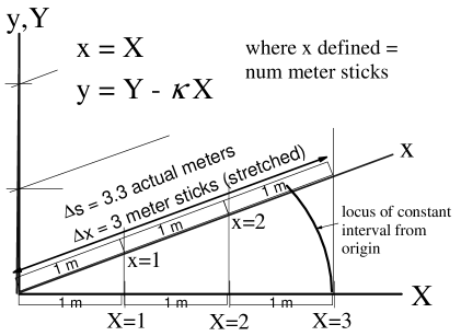
Figure 3: . Artificial (Weird) Spatial Transformation

Note that to enforce this restriction, the meter sticks along the $x$ axis must be stretched, i.e., a meter stick no longer measures one meter of actual length. The number of meter sticks for $\Delta s$ shown in the figure is three, but the physical length of $\Delta s$ is not this, but 3.3 meters. This, no doubt, seems bizarre and certainly runs counter to one’s normal understanding and application of differential geometry. However, as we will show below, this is precisely the sort of thing that happens in the theory of conventionality of synchronization.

5.2 Conventionality of Synchronization

Consider a resynchronization such as that described by Anderson, Vetharaniam, and Stedman[25] (“AVS synchronization”), i.e., (1) with $C$ = 1, analogous to taking the spatial $y,Y$ axes in (18) over to temporal axes ct and cT, and for which $X,T$ comprise an Einstein synchronized coordinate system. This is

$$\begin{array}[]{l}x=X\,\,\,\,\,\,\,\,\,\,\,\,\,\,\,\,\,\,\,\,\,\,\,\,\,\,\,\,\,\,\mbox{where}\,\,x\,\,\mbox{is}\,\mbox{constrained}\,\mbox{to}\,\mbox{equal}\,\mbox{the}\\ ct=cT-\kappa X\,\,\,\,\,\,\,\,\,\,\,\,\,\,\,\mbox{number}\,\mbox{of}\,\mbox{meter}\,\mbox{sticks}\,\,\mbox{along}\,x\,\mbox{axis.}\\ \end{array}$$ (19)

Like the prior example with purely spatial coordinates, this transforms orthogonal coordinate axes to non-orthogonal coordinate axes (see Fig. 4), which in this case are termed non-time-orthogonal. From Fig. 4, one can glean that a greater value of $\kappa$ implies a greater slope of the spatial axis $x$ from the horizontal.

For later reference, we note that, as shown by AVS, the metric for the resynchronized ct-x coordinates is

$$g_{\alpha\beta}=\left[{{\begin{array}[]{*{20}c}{-1\hfill}&0\hfill&\kappa\hfill&0\hfill\\ 0\hfill&1\hfill&0\hfill&0\hfill\\ \kappa\hfill&0\hfill&{1-\kappa^{2}\hfill}&0\hfill\\ 0\hfill&0\hfill&0\hfill&1\hfill\\ \end{array}}}\right],$$ (20)

where for convenience in comparison with other metrics presented herein, we have moved the terms in $\kappa$ from the second row/column to the third (i.e., we have exchanged $x$ and $y$ directions in (20).)

Note that in such resynchronization transformations, the $x$ coordinate in the new coordinate grid is equal to the number of meter sticks from the origin along the $x$ axis. However, this is not equal to the actual interval length $\Delta s$, and it is the latter, not the former, which in differential geometry is considered to be the actual, physically measurable length[43].

See Fig. 4, noting that, unlike the purely spatial transformation of Fig. 3, the presence of a minus sign in the temporal component of the metric means the locus of constant interval length is a hyperbola rather than a circle. Thus, the actual interval distance along the $x$ axis is less than the number of meter sticks. Thus, in a seemingly weird way, lengths measured with physical meter sticks are not physical lengths in the usual differential geometry sense.

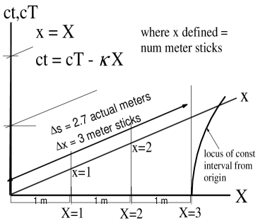
Figure 4: . Synchronization (Space-Time) Transformation

In spacetime (relativistic) theory, proper length is defined as the interval $\Delta s$ along an axis of simultaneity (e.g., the $x$ axis in Fig. 4) and this $\Delta s$ corresponds to the term physical length. With Einstein synchronization, “proper length” is synonymous with “rest length” (the number of meter sticks laid out between, and at rest with respect to, two 3D points.) However, for non-Einstein synchronization, proper length$\Delta s_{t=0}=\Delta\hat{x}$ is not equal to rest length $\Delta x$.

This is a result of the requirement, in conventionality of synchronization theories, that one simply resets clocks at locations separated by constant, meter stick measured, distances. Thus, the values assigned to $x$ in such theories are no longer mere labels with little physical significance, but become pegged to specific values measured with physical instruments in the real world.

The distinction between proper length (actual physical length in 4D differential geometry sense) and rest length (physical in terms of using meter sticks to measure, which we will henceforth call “real world” length) will become important when we investigate arguments for, and against, curvature of the surface of a rotating disk.

Conclusion: For non-Einstein synchronizations, rest length measured via standard real world meter sticks (equal to dx) does not equal proper length (equal to ds along the $x$ axis) in meters. Care must be taken in interpreting differential geometry in 4D, as this ds is defined therein as the “physical component” in the $x$ direction, which in a purely spatial space equals the number of meter sticks needed to traverse it. In 4D, this is only true for Einstein synchronization.

6 Lorentz Contraction and Conventionality of Synchronization

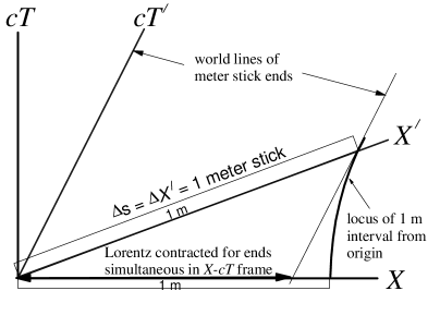
Figure 5: . Lorentz Contraction with Einstein Synch

Fig. 5 serves as a review of the source of Lorentz contraction between two inertial frames in relative motion. The meter stick fixed in the primed frame (with the world lines of its endpoints shown) appears to be moving to an observer in the unprimed frame. Lorentz contraction arises by stipulating that the endpoints of the primed meter stick must be considered simultaneous to the unprimed observer. Thus, with this stipulation, and as illustrated, the unprimed frame observer determines that the moving meter stick is shorter than his own stationary (relative to him) meter stick. The intersection of the moving meter stick endpoint worldlines with the stationary frame spatial axis determines the amount of the contraction. Fig. 5 illustrates this for Einstein synchronized coordinates.

However, as noted in Sec. 5.2, the slope of the (unprimed) spatial axis depends on the observer’s choice of simultaneity. But this means the intersection point of the moving meter stick’s right end worldline with the unprimed spatial axis will be different for different simultaneities in the unprimed frame (see Fig. 6), and thus the length seen in the unprimed frame would depend on the simultaneity chosen therein.

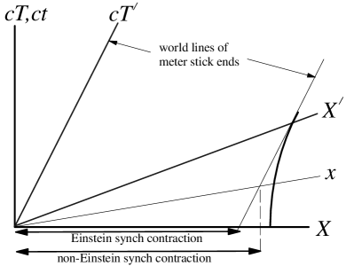
Figure 6: . Non-Einstein Synch Contraction

Thus, if simultaneity is truly conventional, then so is Lorentz contraction. And it follows that, if one insists measurement can be made via Lorentz contracted meter sticks on a rotating disk, there can then be no unique value for the circumference of that disk, nor any unique curvature for the disk surface, as claimed in the traditional approach to relativistic rotation.

Conclusions:

1. Different synchronization (simultaneity) means different Lorentz contracted lengths for the same moving meter stick (using the standard definition of Lorentz contraction.)

2. Conventionality of synchronization and the traditional rotating disk argument for Lorentz contraction leading to a unique, invariant disk curvature cannot both be true.

7 A Complete Analysis: Acceleration Included

A complete general relativistic analysis of a particular problem is not limited to times, lengths, and velocities, but includes accelerations, forces, and curvature as well. Central to all of this is the metric, which one employs in tensor analysis to determine all of these quantities.

7.1 Well Known Examples

7.1.1 Schwarzchild field

Given a suitable metric for a Schwarzchild field (abbreviated form shown in (16)), one can determine not only physically measured (proper) distances between points (see (17), for example), proper times, and physical velocities, but (physical) accelerations of particles, forces, electromagnetic relations, and the Riemann tensor, as well.

7.1.2 Rectilinear acceleration

As shown in Chapter 6 of Misner, Thorne, and Wheeler[42], LCIFs can be used to derive a suitable metric for a frame accelerating in a straight line. Using that metric, one can find all the aforementioned relevant quantities, kinematic, dynamic, and geometric for that frame.

7.1.3 Rotation via transformation theory

In rotation, any viable analytic approach must be able to predict centrifugal and Coriolis accelerations, as well as curvature. Using the most widely employed transformation between the lab and a rotating frame, these things can indeed be determined. This analysis procedure is known, but relatively difficult to find in the literature, and as it is relevant to comments to be made later, I include it here for reference.

For rotation, with familiar symbols for cylindrical coordinates and the coordinate transformation

$$\begin{array}[]{l}ct=cT\quad\quad\quad\quad\quad\mbox{(a)}\\ r=R\quad\quad\quad\quad\;\;\;\quad\mbox{(b)}\\ \phi=\Phi-\omega T\quad\quad\quad\;\,\mbox{(c)}\\ z=Z\quad\quad\quad\quad\quad\;\;\;\mbox{(d)}\\ \end{array},$$ (21)

where upper case refers to the lab frame, and lower case to the rotating frame, the metric and its inverse[44] are

$$g_{\alpha\beta}=\left[{{\begin{array}[]{*{20}c}{-(1-\textstyle{{r^{2}\omega^{2}}\over{c^{2}}})\hfill}&0\hfill&{\textstyle{{r^{2}\omega}\over c\hfill}}&0\hfill\\ 0\hfill&1\hfill&0\hfill&0\hfill\\ {\textstyle{{r^{2}\omega}\over c\hfill}}&0\hfill&{r^{2}\hfill}&0\hfill\\ 0\hfill&0\hfill&0\hfill&1\hfill\\ \end{array}}}\right]\quad g^{\alpha\beta}=\left[{{\begin{array}[]{*{20}c}{-1\hfill}&0\hfill&{\textstyle{\omega\over c\hfill}}&0\hfill\\ 0\hfill&1\hfill&0\hfill&0\hfill\\ {\textstyle{\omega\over c\hfill}}&0\hfill&{(1-\textstyle{{r^{2}\omega^{2}}\over{c^{2}}})/r^{2}\hfill}&0\hfill\\ 0\hfill&0\hfill&0\hfill&1\hfill\\ \end{array}}}\right].$$ (22)

Note from the form of (21)(a), that for this transformation, the lab and the rotating frame have the same simultaneity ($\kappa$ = 0 in (1), so that if $\Delta T$ = 0 between any two events, then $\Delta t$ = 0). Also, $t$ turns out to be a coordinate clock time in the rotating frame, not standard (physical, real world) clock time (which varies from $t$ by the Lorentz factor.)

For (22), the only non-zero Christoffel symbols, found from

$$\Gamma_{\alpha\beta\gamma}=\textstyle{1\over 2}\left({g_{\alpha\beta,\gamma}+g_{\alpha\gamma,\beta}-g_{\beta\gamma,\alpha}}\right),\,\,\,\,\,\,\Gamma^{\alpha}_{\beta\gamma}=g^{\alpha\mu}\Gamma_{\mu\beta\gamma}\,,$$ (23)

are

$$\Gamma^{r}_{tt}=\Gamma^{1}_{00}=-\frac{\omega^{2}r}{c^{2}},\,\,\,\,\,\,\,\,\Gamma^{\phi}_{tr}=\Gamma^{2}_{01}=\frac{\omega}{cr},\,\,\,\,\,\,\,\,\,\Gamma^{r}_{t\phi}=\Gamma^{1}_{02}=-\frac{\omega r}{c}.$$ (24)

The equation of motion for a geodesic particle, in rotating frame coordinates, is

$$\frac{d^{2}x^{\alpha}}{d\tau^{2}}+\Gamma^{\alpha}_{\beta\gamma}\frac{dx^{\beta}}{d\tau}\frac{dx^{\gamma}}{d\tau}=0.$$ (25)

The relevant 4-velocities are

$$\begin{array}[]{l}u^{0}=\frac{dx^{0}}{d\tau}=\frac{cdt}{d\tau}=\frac{c}{\sqrt{1-({v}^{\prime}/c)^{2}}}\\ u^{1}=\frac{dx^{1}}{d\tau}=\frac{dr}{d\tau}\\ u^{2}=\frac{dx^{2}}{d\tau}=\frac{d\phi}{d\tau}\,\,,\\ \end{array}$$ (26)

where ${v}^{\prime}$ is the velocity of the particle as seen in the lab frame (since dt = dT in the first line of (26).)

Radial Direction Acceleration

For the $x^{1}=r$ direction, the equation of motion (25) becomes

$$a^{r}=a^{1}=\frac{\omega^{2}r}{\left({1-({v}^{\prime}/c)^{2}}\right)}+\frac{\omega r}{\sqrt{1-({v}^{\prime}/c)^{2}}}\frac{d\phi}{d\tau}=\underbrace{\frac{\omega^{2}r}{\left({1-({v}^{\prime}/c)^{2}}\right)}}_{Centrifugal\,\,accel}+\underbrace{\frac{\omega\hat{u}^{\phi}}{\sqrt{1-({v}^{\prime}/c)^{2}}}}_{Coriolis\,\,accel}$$ (27)

where $\hat{u}^{\phi}=\sqrt{g_{\phi\phi}}d\phi/d\tau=rd\phi/d\tau$ is the physical (i.e., measured in m/s using standard meter sticks) four-velocity of the particle in the $\phi$ direction relative to the rotating frame. Since the particle is undergoing geodesic motion, as seen from the rotating frame, there is acceleration relative to the rotating frame coordinates. For a particle fixed at constant radius $r$ in the rotating frame, centrifugal and Coriolis pseudo forces equal to the mass times the terms on the RH side of (27) would appear to arise.

The reader who has worked out (24) to (27) realizes that the centrifugal acceleration arises from the $g_{tt}$ term in the metric, whereas the zeroth order Coriolis term in (27) is due solely to the first order time-space component g_tϕ in the metric (22). Without that off-diagonal component due to non-time-orthogonal (NTO) rotating coordinates, we would find no measurable Coriolis acceleration in rotation.

Further, had the simultaneity chosen been other than that of (21)(a) [i.e., with $t$ dependent not only on $T$, but on $\Phi$ as well], then we would have had a different g_tϕ, and thus a different Coriolis acceleration at zeroth order. The Coriolis Newtonian acceleration found in a myriad of experiments and applications is the zeroth order approximation of the value shown in (27). Thus, I submit this to be clear evidence that Nature herself has decided there is no conventionality of simultaneity/synchronization in rotation. The only simultaneity choice producing the known Coriolis effect is that of the lab.

Tangential Direction Acceleration

For the $x^{2}$ = $\phi$ direction, the equation of motion (25) becomes

$$a^{\phi}=a^{2}=\frac{d^{2}\phi}{d\tau^{2}}=-\frac{\omega}{r}\frac{dt}{d\tau}\frac{dr}{d\tau}=-\frac{\omega}{r\sqrt{1-({v}^{\prime}/c)^{2}}}\hat{u}^{r}$$ (28)

where $\hat{u}^{r}=\sqrt{g_{rr}}dr/d\tau=dr/d\tau$ is the physical velocity in the radial direction relative to the rotating frame.

The physical (measured in m/s${}^{2})$ value for the tangential acceleration is

$$\hat{a}^{\phi}=\sqrt{g_{\phi\phi}}a^{\phi}=ra^{\phi}=\underbrace{-\frac{\omega}{\sqrt{1-({v}^{\prime}/c)^{2}}}\hat{u}^{r}}_{Coriolis\,\,accel}.$$ (29)

Again, this zeroth order (Newtonian) term arises solely because we have an off-diagonal first order time-space component in the metric, and is of this value solely because of the particular choice of simultaneity inherent in (21)(a).

Curvature

Since the rotating frame metric was obtained via a transformation from the (flat 4D space) lab metric, Riemann curvature in both 4D frames is zero. For the 2D subspace of the rotating frame, it should be obvious from the r-$\phi$ submatrix of (22) that curvature for that subspace is also zero. This will be discussed in more detail herein, but for the present, we note that this conclusion is conditional, in certain ways, upon our choice of simultaneity, inherent in (21)(a).

Conclusions:

1. The well known zeroth order (Newtonian) Coriolis acceleration found in rotation arises from first order off diagonal time-space terms in the metric, and those terms vary with choice of simultaneity.

2. For any AVS type (first order) synchronization choice having simultaneity other than that of the lab, application of general relativistic principles results in a predicted Coriolis acceleration different at zeroth order from that found in nature.

3. Any transformation differing from (21) only in second order should produce the same zeroth order (Newtonian) Coriolis acceleration.

7.2 Coriolis Acceleration and Rotation via LCIFs

With the traditional LCIF approach to rotating frames, which employs LCIFs with Minkowski metrics, it does not appear that the Coriolis acceleration can be derived. To have Coriolis acceleration, there must be off diagonal t-$\phi$ terms in the metric, such as those in (22). But the traditional LCIF approach, due the imposition of Minkowski coordinates (Lorentz metric) in the LCIF used as a local surrogate for the rotating frame, does not have this characteristic. Thus, it fails as a complete analysis approach to rotating frames. In fact, it is demonstrably quite wrong.

Employing conventionality of synchronization (non-Lorentz metric), however, one can induce a metric in the LCIF that does indeed produce the correct Coriolis acceleration. With the respective line elements from (19) and (22), one can readily show that for the conventionality transformation (1) from Einstein synchronization originally in the LCIF to the appropriate LCIF synchronization, we need $\kappa=v/c^{2}$ (with $C$ = 1), which from (19), is seen to be a first order shift ($v/c)$ in synchronization for time. This, of course, means that synchronization is not conventional for rotating frames, as there is only one synchronization scheme for which theory matches experiment.

Note that this particular synchronization choice is identical to shifting simultaneity in the LCIF to that of the lab, and thus to the choice taken in the transformation (21). This is also equal to the choice advocated in Sec. 2.2.1 herein, as necessary to keep time continuous and single valued.

Conclusion: The only synchronization scheme for the LCIFs that provides complete and correct analysis of rotating systems (including Coriolis acceleration) has the same simultaneity as the lab. This is also the only such scheme that yields continuous, single valued time and clocks in synchronization with themselves in the rotating frame itself.

8 Alternative Theories

We now summarize theories alternative to the traditional LCIF approach, which attempt to resolve the conundrums stated earlier herein. For thorough introduction to each, see Ref. [1] and citations therein.

8.1 Selleri’s Preferred Frame

In his early work[26]^,[27], Selleri used a number of arguments, including the Sagnac experiment, to posit the existence a preferred reference frame, and concomitantly, to an absolute simultaneity shared by all observers. He determined the transformation from the preferred frame to another inertial frame traveling at arbitrary speed $v$ with respect to the preferred frame that upholds these and other experimentally imposed requirements. Using an “S” subscript to refer to a non-preferred frame in the Selleri scheme, non-subscripted capital letters to designate the preferred frame, and a velocity directed along the $X$ axis, this transformation is

$$\begin{array}[]{l}t_{S}=\sqrt{1-v^{2}/c^{2}}\,T\,\,\,\,\,\,\,\,\,\,\,\,\,\,\,\,\,\,\,\,\,\,\,\,\,\,\,\,\,\,(a)\\ x_{S}=\frac{1}{\sqrt{1-v^{2}/c^{2}}}\left({X-vT}\right)\,\,\,\,\,\,\,\,\,\,\,\,\,(b)\\ y_{S}=Y\quad\quad\quad\quad\quad\quad\quad\quad\quad\,\,\,\,\,(c)\\ z_{S}=Z\quad\quad\quad\quad\quad\quad\quad\quad\quad\,\,\,\,\,(d)\,.\\ \end{array}$$ (30)

For future reference, and comparison with other approaches, we note that Selleri’s metric is non-time-orthogonal, and has the form

$$g_{\mu\nu}=\left[{{\begin{array}[]{*{20}c}{-1\hfill}&0\hfill&{v/c\hfill}&0\hfill\\ 0\hfill&1\hfill&0\hfill&0\hfill\\ {v/c\hfill}&0\hfill&{1-v^{2}/c^{2}\hfill}&0\hfill\\ 0\hfill&0\hfill&0\hfill&1\hfill\\ \end{array}}}\right].$$ (31)

For reasons of consistency in comparison with other metrics, we have moved the components arising from the $x_{S}$ coordinate of (30) from the second row and column of (31) to the third.

Note, particularly, that in Selleri’s transformation, like the conventionality transformations discussed in Sec. 5, the coordinates $t_{S}$ and $x_{S}$ represent values measured with physical standard clocks and meter sticks, respectively. But, again like the transformations of Sec. 5, $x_{S}$ does not represent proper length, i.e., it does not represent 4D physical length, the 4D interval length, along the $x_{S}$ axis. See Fig. 7, where along the $x_{S}$ axis an observer fixed to that axis would lay down 3.3 meter sticks to cover a 4D physical length of 3.0 meters.

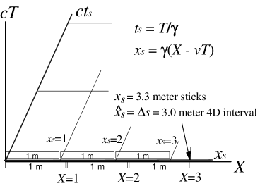
Figure 7: . Selleri Transformation

This means that observers in both frames would consider meter sticks fixed in the $S$ frame to measure $C\neq$ 2$\pi r$.

As Selleri showed, within the S system, one-way speed of light is anisotropic, but the two-way speed remains isotropic and equal to $c$. As many have pointed out[25], distant clock synchronization and one-way light speed are interdependent, so no absolute determination of one-way speed can be made, and thus Selleri’s transformation appears consistent with all possible real-world measurements.

Selleri proposed his transformation for both translation and rotation. But he considered the Sagnac experiment, with its ostensible difference in one-way light speeds, to be a key pillar supporting it. In that test, the distant clock is actually the same as the original clock, and reasonable arguments can be made that it provides a valid measurement of one-way speed.

Note that for application to rotation, with reference to cylindrical coordinates such as those in (21), $v=\omega r$, and the $x_{s}$ direction in (30) is taken as the circumferential, or $\phi$, direction, though it is a measure of distance and not angle. The reader should be aware that, in this case, (31) is not a true rotating frame metric because it is only applicable, as written, along a single circumferential line. For applicability to the entire rotating frame, the metric would need an $r$ dependence, and would be significantly more complicated than (31) (See Sec. 13.2.2.).

Selleri has modified his position recently, and we review this development in Sec. 9.1.

To summarize:

Michelson-Morley

Selleri’s approach predicts a null MM signal.

Lorentz Contraction

Selleri predicts circumferential Lorentz contraction effects in the rotating frame.

Time Gap and Coriolis

Because Selleri’s simultaneity (see (30), first line) equals that of the lab, there is no discontinuity in time such as that shown in Fig. 1. If his metric (31) could be recast as a global metric (with $r$ dependence), like that of (22), his approach would predict a Coriolis acceleration in agreement with the low speed value.

Other Issues Raised by Selleri

It should be mentioned that Selleri has raised other challenges to accepted tenets of SRT, including starlight aberration in inertial reference frames and certain aspects of relativistic acceleration. These deserve serious consideration, but will not be addressed herein.

8.2 Rizzi, Ruggiero, and Serafini’s Desynchronization

Rizzi, Ruggiero, and Serafini[2]^,[19]^,[18] (RRS) have noted that slow (relative to the rotating disk) transport of standard clocks 360^o around the circumference of a rotating disk leads to a time difference between the traveled clock and the clock left at the starting point.

This desynchronization effect has, in fact, been shown by Anderson et al[25] to be generally characteristic of slowly transported clocks in any non-Einstein synched coordinate system. That is, unless the 4D coordinates employ Einstein synchronization, slow transport of any standard clock will yield a time difference (a desynchronization) between that clock and the standard clock at the destination point. For Einstein synchronization, the traveled and destination clocks are in synch.

So if one assumes Einstein synchronization around the rim of the rotating disk, then a slow clock transport around that rim results in no desynchronization between the destination clock (at 360${}^{o})$ and the traveled clock. However the clock at 360^o is out of synchronization with the clock at 0^o (because they have been Einstein synched – see time gap of Fig. 1), and thus the traveled clock is desynchronized with the original starting point clock. Quantitatively, the amount of the desynchronization equals the time gap of Fig. 1.

For clocks traveling slowly in the cw and ccw directions, the difference between those two clocks after 360^o equals the Sagnac time difference (4). That is, both clocks are “desynchronized” from the clock left at the starting point, and the amount of this desynchronization difference turns out to be equal to the Sagnac difference. For these authors, this is the “physical root” of the Sagnac effect, and they thus suggest that this resolves the issue.

However, the coinciding of slow moving clock desynchronization, the Sagnac time difference, and the time gap of Fig. 1 (including the cw equivalent of Fig. 1), do not, I submit, resolve the inconsistency issues of Sec. 2.2 (time discontinuity, limit case, Lorentz contraction) or the Coriolis issue with LCIFs of Sec. 7.2. Further, even for the limited issue involving Sagnac, one could make other arguments for why these three phenomena converge quantitatively.

The transformation used in desynchronization is twofold. First, one transforms using the Lorentz transformation from the lab to the LCIF frame, which is assumed via the principle of locality to reflect the rotating frame itself (locally.) Second, if one chooses, one can resynchronize the LCIF (the rotating frame) via the resynchronization transformation (19) and obtain the metric (20), repeated here for convenience,

$$g_{\alpha\beta}=\left[{{\begin{array}[]{*{20}c}{-1\hfill}&0\hfill&\kappa\hfill&0\hfill\\ 0\hfill&1\hfill&0\hfill&0\hfill\\ \kappa\hfill&0\hfill&{1-\kappa^{2}\hfill}&0\hfill\\ 0\hfill&0\hfill&0\hfill&1\hfill\\ \end{array}}}\right].$$ (32)

In (32), the resynchronization direction is oriented along a circumference and similar to the Selleri case is a distance, not angle, measure. For zero resynchronization from Einstein synchronization, $\kappa$ = 0, and (32) reduces to the Lorentz (or Minkowski) metric. As RRS have shown, regardless of the synchronization chosen (regardless of the form of the metric), the time on a slow moving (with respect to the rotating frame) clock will always turn out to be the same value, i.e., it is invariant with respect to resynchronization transformations.

To summarize:

Michelson-Morley

The RRS desynchronization approach predicts a null MM signal.

Lorentz Contraction

RRS appear to accept circumferential Lorentz contraction, deduced via the traditional logic, which is challenged herein in Secs. 2.2.3 and 6.

Time Gap and Coriolis

RRS advocate conventionality of simultaneity in the rotating frame and thus will have a time discontinuity that varies with choice of simultaneity. For the one choice of simultaneity equal that of the lab, there would be no such discontinuity and clocks would be in synchronization with themselves.

The RRS desynchronization approach will yield different Coriolis type accelerations for different choices of simultaneity. Only for the continuous time choice will it equal the classical, low speed value.

8.3 Bel’s Optical and Mechanical Metrics

Bel[39]^,[45]^,[46]^,[47], along with colleagues, contended that two metrics exist, one optically based, and one mechanically based. In a rotating frame these would turn out to be different, and this difference would manifest as a non-null Michelson-Morley result.

Quantitatively, this non-null signal would be quite close to the anomalous signal measured by Brillet and Hall. Bel notes[48] that according to his analysis, in the earth fixed frame, this signal must be 13^o from the E-W direction, but regrettably, the phase angle of the Brillet-Hall signal was not recorded. Had it been found to be in the direction predicted, it would have lent strong support to Bel’s theory. Of course, a direction other than this would disprove his theory.

Likewise, and similar to Klauber’s approach (to be described below), a null rotating frame MM signal (which would show Brillet-Hall’s signal truly was spurious) would also negate Bel’s approach.

To summarize:

Michelson-Morley Experiment

The Bel et al approach predicts a non-null MM signal close to that found by Brillet and Hall.

Byl et al Experiment

The Byl et al[49] experiment, a presumed first order test of SRT, entailed a one way propagation of light through air and glass. I believed their null result disproved Bel’s approach, but was informed by Bel that it does not, though I am not convinced, as I have not seen an analysis supporting this contention.

Lorentz Contraction, Time Gap, and Coriolis

I have not investigated these issues with regard to the Bel et al approach.

8.4 Nikolic’s Local Proper Coordinate Frames

Nikolic[50] analyzes rotating frames by employing a different local frame with proper coordinates for each rotating frame observer. Adopting terminology from Misner, Thorne, and Wheeler, he presently calls these “proper coordinate frames”, although in past work, he deemed them “Fermi frames”. Actual measurements made in these local frames would equal coordinate values, since coordinate values are purposely chosen to equal proper values.

Nikolic believes the rotating frame cannot be correctly described by a single coordinate system, but only by an infinite set of local proper coordinate frames. He states “even if there is no relative motion between two observers [fixed on a rotating disk, for example], they belong to different frames if they do not have the same position.”[51] Further, he considers this generally true of all non-inertial systems, “two observers at different positions but with zero relative velocity may be regarded as belonging to the same coordinate frame only if they move inertially in flat space-time.”

The reader must read Nikolic directly to gain full appreciation of his justification for this seemingly strange position. We do note that, given this position, he may appear to resolve certain conundrums involving relativistic rotation. For example, if there can be no global frame, then one might argue there is no global time gap issue. However, some, including myself, may not consider this a resolution, as all measurements made in the physical world are of necessity global, and to make predictions, one must integrate over adjacent local frames (as in the traditional LCIF approach). Carrying out such integration for time, Nikolic’s local frames yield a time gap such as that shown in Fig. 1.

Nikolic also presents interesting perspectives on length contraction and clock rates. He argues that “one can study the relativistic contraction in the same way as in the conventional approach with Lorentz frames”. (See Secs. 2.2.3 and 6 herein for reasons why this may not be reasonable.) He also deduces the time seen by an observer on the rotating frame, which is seen to oscillate with each rotation, and only when averaged over a whole rotation, does it equal the traditional Lorentz dilated value.

Nikolic’s metric, expressed in local, not global coordinates, with non-rotation induced accelerations taken as zero and Cartesian coordinates transformed to cylindrical coordinates, is

$$g_{\mu\nu}=\left[{{\begin{array}[]{*{20}c}{-\left({1-\left({{\omega}^{\prime}{r}^{\prime}/c}\right)^{2}}\right)\hfill}&0\hfill&{\left({{\omega}^{\prime}{r}^{\prime}/c}\right){r}^{\prime}\hfill}&0\hfill\\ 0\hfill&1\hfill&0\hfill&0\hfill\\ {\left({{\omega}^{\prime}{r}^{\prime}/c}\right){r}^{\prime}\hfill}&0\hfill&{\left({{r}^{\prime}}\right)^{2}\hfill}&0\hfill\\ 0\hfill&0\hfill&0\hfill&1\hfill\\ \end{array}}}\right]$$ (33)

where primes indicate values in the local coordinate system. The presence of the extra $r^{/}$ in the off diagonal components of (33) (compared to (31), for example) turns the angular $d\phi$ term in the position vector to the distance rd$\phi$ term in the line element.

Note that at the origin of each local frame, $r^{/}$ = 0, and (33) becomes the time-orthogonal Lorentz metric (effectively, for cylindrical coordinates). As one moves away from the local origin, the coordinates become more and more non-time-orthogonal. Thus, a point slightly removed from the origin of the local frame would have a different metric from that of the local frame with its origin at that point.

From the analysis of Sec. 7.1.3, one should be able to see that the derivatives in the calculation of the Christoffel symbols manifest acceptable Coriolis and centrifugal acceleration terms. This is true even though, at the local origin, the metric is diagonal and Lorentzian, similar in this regard to the traditional LCIF approach (which does not yield Coriolis acceleration.)

To summarize:

Michelson-Morley

Nikolic’s approach predicts a null MM signal.

Lorentz Contraction

Nikolic seems to argue that the traditional logic for Lorentz contraction can be applied.

Time Gap and Coriolis

Nikolic shows a time discontinuity globally, if one integrates his local frame time values around the entire circumference. His metric does give rise to the correct low speed Coriolis acceleration, and to centrifugal acceleration.

8.5 Klauber’s NTO Approach

Klauber[16]^,[40]^,[44] analyzed relativistic rotation using a fully differential geometric approach. He started with the widely used transformation to a rotating frame (21), i.e.,

$$\begin{array}[]{l}ct=cT\quad\quad\quad\quad\quad\mbox{(a)}\\ r=R\quad\quad\quad\quad\;\;\;\quad\mbox{(b)}\\ \phi=\Phi-\omega T\quad\quad\quad\;\,\mbox{(c)}\\ z=Z\quad\quad\quad\quad\quad\;\;\;\mbox{(d)}\,\mbox{,}\\ \end{array}$$ (34)

which yields the non-time-orthogonal (NTO) rotating frame metric (22), i.e.,

$$g_{\alpha\beta}=\left[{{\begin{array}[]{*{20}c}{-(1-\textstyle{{r^{2}\omega^{2}}\over{c^{2}}})\hfill}&0\hfill&{\textstyle{{r^{2}\omega}\over c\hfill}}&0\hfill\\ 0\hfill&1\hfill&0\hfill&0\hfill\\ {\textstyle{{r^{2}\omega}\over c\hfill}}&0\hfill&{r^{2}\hfill}&0\hfill\\ 0\hfill&0\hfill&0\hfill&1\hfill\\ \end{array}}}\right].$$ (35)

He then used tensor analysis with that metric to deduce relevant properties of rotating frames.

To find light speeds, Klauber set the line element for ds found from (35) equal to zero for two conditions: 1) circumferential direction (dr = dz = 0), and 2) radial direction ($d\phi$ = dz = 0.) These equations could then be solved for 1) d$\phi$/dt and 2) dr/dt.

He then assumed the standard differential geometry approach for finding physical components (those measured with actual instruments according to the theory) applied and found the one-way physical velocity (see (14)) in the circumferential direction to be

$$v_{light,phys,circum}\;\;=\;\;\frac{\sqrt{g_{\phi\phi}}d\phi}{\sqrt{-g_{tt}}dt}\;\;=\;\;\frac{-\;\omega r\;\pm\;c}{\sqrt{1-\textstyle{{\omega^{2}r^{2}}\over{c^{2}}}}}=\;\;\frac{-\;v\;\pm\;c}{\sqrt{1-\textstyle{{v^{2}}\over{c^{2}}}}},$$ (36)

and the one-way physical radial direction velocity to be

$$v_{light,phys,radial}=\frac{d\hat{r}}{d\hat{t}}=\frac{\sqrt{g_{rr}}dr}{\sqrt{-g_{tt}}dt}=c.$$ (37)

Using (36) and (37) in the standard MM analysis[40], Klauber found a time delay in the circumferential direction over that in the radial (and $z$ direction) of $\raise 2.15277pt\hbox{$\scriptstyle 1$}\kern-1.00006pt/\kern-1.49994pt\lower 1.07639pt\hbox{$\scriptstyle 2$}v^{2}$/$c^{2}$, and thus an expected non-null MM signal very close to that found by Brillet and Hall.

Klauber also reasoned that the method for finding physical components from differential geometry should allow ready determination of whether or not Lorentz contraction exists in a rotating frame. Thus,

$$\begin{array}[]{l}\mbox{measured}\,\,\mbox{length}\,\,\mbox{in}\,\,\mbox{rotating}\,\,\mbox{frame}\,\,\mbox{=}\,\,d\phi_{phys}\\ =d\hat{\phi}=\sqrt{g_{\phi\phi}}d\phi=rd\phi=r(\phi_{2}-\phi_{1})\\ \end{array},$$ (38)

which from (34), with endpoint measurements simultaneous (i.e., $t_{1}$ = $t_{2}\to$ $T_{1}=T_{2})$, equals

$$\begin{array}[]{l}R\left({\Phi_{2}+\omega{\kern 1.0pt}{\rm T}_{2}-\Phi_{1}-\omega{\kern 1.0pt}{\rm T}_{1}}\right)=R\left({\Phi_{2}-\Phi_{1}}\right)\\ =\,\mbox{measured}\,\,\mbox{length}\,\,\mbox{in}\,\,\mbox{lab}\\ \end{array}.$$ (39)

Thus, if the measured length between two 3D points is the same in both the rotating frame and the lab, there is no Lorentz contraction. Note that, via this logic, we would need a metric with $g_{\phi\phi}\neq r^{2}$ to have Lorentz contraction.

To summarize:

Michelson-Morley Experiment

Using differential geometry with physical component determination, Klauber predicted a non-null MM signal close to that found by Brillet and Hall.

Byl et al

At first perusal, one might consider Klauber’s approach disproved by the Byl et al[49] result, but a thorough analysis[52] showed this not to be the case.

Lorentz Contraction

Using the same differential geometric approach, Klauber predicted no Lorentz contraction and $C$ = 2$\pi r$.

Time Gap and Coriolis

Similar to Selleri, simultaneity in the rotating frame and the lab are the same, so there is no discontinuity in time such as that shown in Fig. 1. Klauber contends there is only one correct simultaneity in rotation, the one for which no time discontinuity exists. Coriolis acceleration determination is correct in the low speed limit, as shown in Sec. 7.1.3. Centrifugal acceleration is also found correctly.

Analysis Depends on Two Things:

All of Klauber’s predictions depend on two things: 1) correctness of transformation (34) (i.e., is this the actual transformation nature has chosen?) and 2) physical lengths as determined using differential geometry equal those actually measured with real world meter sticks.

9 Convergence of Seemingly Disparate Theories

9.1 Synchronization Conventionality Means Selleri = SRT for Inertial Frames

In an enlightening article[2], RRS show that, accepting conventionality of synchronization as true, Selleri coordinates in any non-preferred Selleri inertial frame can be converted into Minkowski coordinates (i.e., the frame is actually a Lorentz frame). If the non-preferred Selleri frame has velocity $v$ relative to the preferred frame, then resynchronization with $\kappa$ = $v/c$, i.e.,

$$ct_{M}=ct_{S}-(v/c)x_{S}\quad,$$ (40)

will transform the Selleri coordinates to Minkowski coordinates. Graphically, this is illustrated in Fig. 8, where the non-time-orthogonal Selleri coordinates ct${}_{S}-x_{S}$ are shown converted to orthogonal (Minkowski) coordinates ct${}_{M}-x_{M}$.

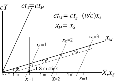
Figure 8: . Synch Transformation for Selleri Coords

Thus, any inertial frame proposed by Selleri as non-preferred can in reality be chosen as his preferred frame (i.e., the frame with isotropic one-way light speed.) And thus, there can be no true preferred frame. Selleri[3] now agrees with this, though he has some difference with RRS on philosophic and interpretational levels.

RRS then extend this logic to rotating frames, and surmise that the difference between Selleri’s approach and the traditional LCIF approach is simply a choice of simultaneity, and that any such choice works, though some may be more convenient for certain problems than others. From this point of view, they consider Selleri’s limit case speed of light paradox (Sec. 2.2.2) to be no paradox at all, but merely arises due to differing choices for simultaneity in the rotating and LCIF frames.

While I agree wholeheartedly with the analysis by RRS with regard to inertial frames, I disagree with regard to rotating frames. For reasons delineated herein, I consider Selleri’s choice of simultaneity to be the only feasible one on a rotating platform.

Conclusion:

Any inertial frame originally proposed by Selleri as non-preferred can be shown, via a shift in simultaneity, to be a Lorentz frame, and thus no unique preferred frame actually exists. RRS consider this result applicable to non-inertial, and in particular rotating, frames, and thus contend that Selleri’s approach is essentially equivalent to their own (LCIFs with conventionality of simultaneity.)

9.2 Klauber Similar to Selleri for Rotation

9.2.1 Time for Selleri and Klauber

Selleri’s original approach, as applied to rotation, and Klauber’s approach share the principle that simultaneity in the rotating frame is the same as that in the lab. Clocks run at different rates in the rotating frame, but observers in both frames can agree that zero time passes on their clocks between two spatially separate events.

The rates on physical standard clocks are also the same for both approaches. The difference is only in the definition of coordinate time. For Selleri, using (31) and (30), a standard clock fixed in the rotating frame has

$$\begin{array}[]{c}\mbox{Selleri}\,\mbox{standard}\mbox{ clock}\,\mbox{time}\,=d\hat{t}_{S}=\sqrt{-g_{S\,tt}dt_{S}dt_{S}}\\ =\sqrt{-(-1)dt_{S}^{2}}=dt_{S}=\sqrt{1-(\omega r)^{2}/c^{2}}dT\,,\\ \end{array}$$ (41)

and his coordinate time equals the time on a standard clock at a given location.

For Klauber, coordinate time corresponds to time on a clock located at the center of rotation. From (35),

$$\begin{array}[]{c}\mbox{Klauber}\,\mbox{standard}\mbox{ clock}\,\mbox{time}\,=d\hat{t}_{K}=\sqrt{-g_{K\,tt}dt_{K}dt_{K}}\\ =\sqrt{-(-1+(\omega r)^{2}/c^{2})dt_{K}^{2}}=\sqrt{1-(\omega r)^{2}/c^{2}}dT\,,\\ \end{array}$$ (42)

and thus, (41) equals (42).

Conclusion: The Selleri and Klauber approaches, in terms of predictions for physically measured time, are essentially equivalent. Both have the same simultaneity, degree of non-time-orthogonality (slope of time axis), and time dilation.

9.2.2 Space for Selleri and Klauber

With regard to distances measured with standard (physical) meter sticks, however, the definition of the spatial coordinate in the circumferential direction becomes critical. As shown in Sec. 8.1, and illustrated in Fig. 7 therein, Selleri defines his $x_{S}$ coordinate (in similar fashion to his choice of time coordinate) as equal to the value measured with actual physical meter sticks. Via his transformation (30)(b), the Lorentz contraction of those meter sticks is then “built in”. Given the definition of $x_{S}$, and Selleri’s chosen transformation, Lorentz contraction in the rotating frame, agreed to by all observers in all frames, must result.

We note that this choice of transformation is built on a prejudice that we must have Lorentz contraction in the rotating frame. And this prejudice is based on the traditional, widely dispersed logic, which, is suggested in Secs. 2.2.1, 2.2.3 and 6, to be inconsistent. Lorentz contraction in rotation may exist, but there is no sound theoretical reason to insist, a priori, that it must. Only experiment can answer this question unequivocally.

With regard to space, Klauber and Selleri have two differences, one trivial, one not so. Trivially, Klauber uses cylindrical coordinates with d$\phi$ in the circumferential direction, whereas Selleri uses orthogonal coordinates and dx_s in the circumferential direction.

Non-trivially, Selleri takes his coordinate value dx_s as equal to the number of real world meter sticks (and not ds), whereas Klauber, in the usual differential geometry fashion, considers ds to be the distance measured in real world meter sticks, with d$\phi$ merely a coordinate value. Thus, we have

$$\begin{array}[]{l}\mbox{Selleri}\,\mbox{interval}\,\,=ds=\sqrt{1-\omega^{2}r^{2}/c^{2}}dx_{s}\\ \mbox{Selleri}\,\mbox{real}\,\mbox{world}\,\mbox{meter}\,\mbox{sticks}\,\,=dx_{s}\,\,\left({\neq ds}\right)\\ dx_{s}=\frac{1}{\sqrt{1-\omega^{2}r^{2}/c^{2}}}dX=\mbox{Lorentz}\,\mbox{contracted}\,\mbox{measure,}\\ \end{array}$$ (43)

and

$$\begin{array}[]{l}\mbox{Klauber}\,\mbox{interval}\,\,=ds\,\,\,\,\,\left({\mbox{same}\,\mbox{as}\,\mbox{Selleri}}\right)\\ \mbox{Klauber}\,\mbox{real}\,\mbox{world}\,\mbox{meter}\,\mbox{sticks}\,\,=ds=\sqrt{g_{\phi\phi}}d\phi=rd\phi\\ ds=Rd\Phi\,=\,\mbox{no}\,\mbox{Lorentz}\,\mbox{contraction}\,\mbox{measurement.}\\ \end{array}$$ (44)

Note that if Klauber were to assume at the outset, as Selleri did, that Lorentz contraction of meter sticks must exist, then one would simply, and alternatively, reinterpret ds = rd$\phi$ as a number not equal to the number of real world meter sticks used to measure distance. That is, as

$$rd\phi=\sqrt{1-\omega^{2}r^{2}/c^{2}}\underbrace{dx_{K}}_{\begin{array}[]{l}\mbox{meter}\,\mbox{sticks}\\ \mbox{for}\,\mbox{alternative}\\ \mbox{Klauber}\\ \end{array}}=\sqrt{1-\omega^{2}r^{2}/c^{2}}\underbrace{dx_{S}}_{\begin{array}[]{l}\mbox{meter}\,\mbox{sticks}\\ \mbox{for}\,\mbox{Selleri}\\ \end{array}}.$$ (45)

Thus, the difference between Selleri and Klauber, with regard to spatial measurements, is solely one of interpretation. If one insists on Lorentz contraction (because presumably it has been found experimentally in rotation), then it is merely an issue of reinterpreting Klauber’s coordinates in terms of real world meter sticks, which are a priori assumed to contract.

Conclusions:

1. The Selleri and Klauber approaches, in terms of predictions for real world measured lengths, can be considered essentially equivalent, if one assumes ahead of time that Lorentz contraction of real world meter sticks exists. Any difference then lies solely in interpretation of coordinate values.

2. Klauber originally used the standard differential geometry interpretation (for purely spatial spaces) of the interval ds as equal to the number of real world meter sticks. For this interpretation, there is no Lorentz contraction.

9.3 Are All Approaches Equivalent?

If the Selleri approach, given conventionality of synchronization, is equivalent to the traditional, or RRS, approach, and the Klauber approach is equivalent to the original Selleri approach, then one could ask if all approaches converge to the same theory. There are two aspects to the answer.

First, it does not appear that the Bel or Nikolic approaches can be enveloped into the fold. They seem distinctly different from the other three.

Second, if there is only one possible simultaneity in rotation, as is argued herein, then the Selleri approach is not equivalent to the RRS approach. The original Selleri approach and the Klauber approach would remain equivalent, varying only in the interpretation of coordinate values with regard to real world measurements of Lorentz contraction, if any.

Conclusion: With regard to time and space, the (original) Selleri and Klauber approaches are equivalent (variation can occur in interpretation.) Selleri’s approach can be extended to be equivalent to RRS only if simultaneity in rotation is conventional.

10 A Complete Consistent Theory of Rotation?

10.1 Need for Global Metric and Unique Time in a Good Theory

The standard general relativistic approach can be summarized as the following.

Lay out a 4D coordinate grid, i.e., a 3D coordinate grid plus coordinate clocks at each point in the 3D grid. Using standard real world meter sticks and real world clocks at each 3D point, make measurements and determine the metric everywhere for the 4D grid chosen. (Note that the simultaneity scheme to be used is inherent in the clock settings chosen, and once the settings are made, every event has a unique time associated with it.)

This metric is then used with all laws of physics, generalized covariant laws - kinematic, dynamic, electromagnetic, gravitational - to deduce all observed phenomena. Additionally, the global geometry can be found by using the metric to determine the Riemann tensor.

Thus, a good and complete theory has

1. a global metric, and

2. a unique time at each event (unique clock at each 3D point).

Note that 2) above is contrary to approaches to rotation that allow more than one time to be assigned to a given event, for a single specific synchronization scheme.

10.2 A Good Global Metric for Rotation Must Exist

Thus, there must exist a good global theory for rotation, as we can certainly climb aboard a rotating disk with standard meter sticks and clocks in hand, lay out a grid on the disk and have a metric which can be used to deduce all phenomena. Without such a coordinate grid and metric, it would not be easy, for example, to solve for the trajectory of a particle (free or not) as seen by an observer on a rotating disk. If we have a global coordinate system, we can specify the position coordinates as functions of time and have a very compact description, of enormous practical value, of the particle motion. How does one do that if the particle is crossing into a new coordinate system (infinitesimal, local) at every instant? It can probably be done, but the work doing it, and the final expression(s) showing it, are complex to extraordinary degree.

Thus, I claim that the best (i.e., the simplest, most straightforward) theory of rotation is one with a global metric inherent within that theory. The overriding question then should be “what is a valid form for that metric?”

Note that this metric, if we are to obey the usual rules of GR physics, must have continuous, unique time values throughout. Note also, that the traditional approach of local LCIFs has not been shown to provide a global metric, suitable for solving all rotating frame problems.

11 2005 Experiments

Three experiments expected to be crucial in deciding between Bel/Klauber type theories, which predicted non-null MM rotating frame signals, and others, were reported in 2005. However, with respect to the issue addressed herein of culling incorrect theories of rotation from the extant mix, two of these experiments, as originally reported, did not provide an answer to this question.

Each of the three experiments utilized a rotating apparatus and was a variation on the standard MM experiment. Their sensitivities were more than sufficient to detect any non-null signal due to the earth surface speed about its own axis, which would be of the order 10^-13. However, the primary focus in each experiment was to determine cosmic anisotropies in light speed (i.e. relative to the fixed stars, not the earth surface), and the method used to analyze this can completely obscure any local effect from the earth surface speed due to its rotation.

Figure 9: . Expected Data for Rotation Anisotropy

To see this, consider Fig. 9, which displays the type of data (but not the actual data) found by Brillet and Hall[38], and illustrated in Fig. 2 of their report. Data is taken over one rotation of the earth (24 hours) and can be plotted in two ways, using “+” symbols as relative to the fixed stars, and using “o” symbols relative to the earth’s surface. Averaging the former nets an effectively null signal, i.e., zero cosmic anisotropy. Averaging the latter nets a significant non-null signal, suggestive of local anisotropy. This is the type of signal that occurred in the Brillet and Hall data, and though considered anomalous by most, was cited by Bel and Klauber as a possible indication of true anisotropy in the rotating earth frame. The magnitude of this local signal found by Brillet and Hall was remarkably close to what one would expect from a pre-relativistic analysis using the surface speed of the earth about its axis as the “ether” speed.

However, as we will see below, data from at least two of the 2005 tests showed something different.

11.1 Antonini et al

Antonini et al[4] compared the resonance frequencies of two perpendicular optical resonators as their apparatus rotated relative to the lab. They took data samples at 1 second intervals for 76 hours. They first analyzed their data as a function of one resonator’s axis relative to the south direction to obtain amplitudes for each individual rotation of their apparatus.

This is precisely the type of analysis needed for our purpose, and it showed variations on the order of 10^-14, approximately an order of magnitude smaller than the anomalous Brillet and Hall signal and thus, that required by Bel and Klauber.

Antonini et al then plotted the single rotation signal amplitudes against hours of test duration to discern any cosmic anisotropy (which would manifest as changes over several hours as the earth alignment with the heavens changed), and found no evidence for it.

Conclusion: Antonini et al analyzed data in the earth fixed frame and found no signal such as that of Brillet and Hall, which might indicate rotating frame anisotropy of light speed.

11.2 Stanwix et al

Stanwix et al[5] rotated two orthogonally oriented cryogenic resonator-oscillators operating in whispering gallery modes to test for violations of Lorentz invariance. They found nothing to suggest light speed anisotropies, but unfortunately, for our purpose, the original analysis of their data was carried out entirely in the non-rotating earth centered frame. The computer driven analysis converted all data to this frame before analysis, and thus the results are meaningless with regard to determination of LLI violation in rotation.

Stanwix has indicated he may re-evaluate their data in the earth-fixed frame, but as of this writing, he has not been able to do so.

Conclusion: In their report, Stanwix et al analyzed data in the sidereal frame, so their results are inconclusive for our purpose.

11.3 Herrman et al

Herrman et al[6] tested Lorentz invariance by comparing resonance frequencies of a continuously rotating optical resonator with a stationary one. Although it is not obvious from their report, in personal communication, Herrman kindly provided greater detail of their analysis procedure, including data plotted in a manner similar to that of Fig. 9. Any possible constant lab frame phase signal was significantly less than an order of magnitude smaller than that found by Brillet and Hall.

Conclusion: The Herrman et al data, analyzed in the earth fixed frame, indicates no anisotropy such as that suggested by the anomalous Brillet and Hall signal.

11.4 Summary of Four Experiments

As neither the Antonini et al nor Herrmann et al experiments show an earth-fixed frame non-null MM type signal, which would suggest local light speed anisotropy, it is highly probable that the Brillet and Hall anomalous signal truly was attributable to mundane cause. Brillet and Hall did not have the advantage of later generation technologies for monitoring such things as apparatus tilt, whereas all of the recent researchers did. The Stanwix et al experiment is inconclusive as of this writing, though further analysis, appropriate to this issue, is expected.

Conclusion: It is all but certain that back and forth light speed in rotating frames is isotropic.

12 Evaluation of Proposed Theories of Rotation

12.1 Summary of Pros and Cons

Table 1 shows the proposed theories of relativistic rotation (see Sec. 8) vs. their significant characteristics, their agreement or lack thereof with key experiments, and their consistency with regard to certain theoretical issues.

Note that the Selleri theory considered is his original one, which I believe continues to have merit for rotation (though has been subsumed into the conventionality thesis for translation.). Question marks signify my ignorance with regard to what the particular theory would say, as the topic appears to not have been treated in published work by the respective author.

Table 1: Comparison of Proposed Theories

	RRS SRT	Selleri Original	Klauber NTO	Bel 2 Metrics	Nikolic Local
Reference frame	LCIF	Local	Entire rotating frame	Entire rotating frame	Local proper frames
Simultaneity	Convention	= Lab	= Lab	?	Einstein
Global metric?	No	No	Yes.	Yes. Two: optical & mechanic	No.
Experiment
Time dilation?	Yes	Yes	Yes	Yes	Yes
Predicts Sagnac? (correct $\Delta$ time)	For $\kappa$ $=v/c$ (or resync)	Yes	Yes	Yes	Yes
Antonini/Herrman? (= MM Lorentz contraction)	Yes	Yes	No	No	Yes
Brillet & Hall? (= no Lorentz contraction)	No	No	Yes	Yes	No
Coriolis effect derivable? (= continuous time)	No	Yes	Yes	?	Yes (but discontinuous time)
Byl et al?	Yes	Yes	Yes	?	Yes
Consistent with:
Continuous time? (clock synched with itself)	Only for $\kappa$ $=v/c$	Yes	Yes	?	?
Large radius limit case? ($\omega r$ const, $\omega\approx$ 0)	Yes, if simultaneity conventional	Yes	Yes	?	Yes

12.2 Which Theory (Theories) Work(s)?

12.2.1 If Brillet and Hall local signal represents reality

If the anomalous Brillet and Hall signal indicates a genuine attribute of physical law, which is doubtful, then only the Bel and Klauber approaches would be viable.

12.2.2 If Antonini/Herrmann data represent reality

If, as is almost certain, the Antonini et al and Herrmann et al results, showing no local anisotropy, represent physical law, then the Bel and Klauber approaches, at least in their original incarnations, are not correct. As the recent researchers took advantage of innovations in monitoring technology not available to Brillet and Hall to measure apparatus tilt (the likely cause of the Brillet and Hall non-null local signal), it appears prudent to consider the recent experiments as the more representative of physical law, in the following consideration of the remaining theories.

RRS

The RRS approach embraces conventionality of synchronization in rotation, but the analysis of Sec. 7.2 shows that only one synchronization scheme produces the Coriolis acceleration found in the Newtonian limit. This analysis appears to be the death knell for conventionality in rotation, and thus also for the RRS approach.

Further, the RRS approach does not provide a global metric, which, it is argued in Sec. 10, is fundamental for a general relativistic description of any physical system.

Nikolic

Nikolic would pass the appropriate Coriolis acceleration test, at least locally, and it seems other criteria as well. However, his basic tenet that a rotating frame does not represent a single frame, for the purposes of general relativistic analysis, appears weak. It does not meet the need, as described herein, for a global metric requisite for complete analysis of any physical system.

Why, for example, can one not employ the plan of Sec. 10.1? Certainly, one can climb aboard a rotating disk, with meter sticks and clocks in hand, lay out a coordinate grid, determine a global metric, and use it to analyze any physical situation. I consider any system where one can do this as a valid general relativistic frame, though Nikolic prefers the local proper frame for studying the physical effects viewed by a local observer. While Nikolic’s approach may be more convenient for less simple spacetimes, for the flat spacetime of rotation, I believe the global metric approach to be more convenient, and thus preferable.

Selleri

Selleri has the requisite, unique simultaneity necessary to predict the correct Coriolis acceleration, and also agrees with Antonini et al (i.e., Lorentz contraction exists.) However, his theory, as relates to rotation, comprises only a local $x-y-z-t$ frame with a local metric, rather than a global frame with global metric.

I suggest that the Selleri approach is valid, but that it lacks a general relativistic underlying structure to deal with all problems in rotation (i.e., it lacks a global metric.) We shall see that a combination of Selleri’s approach with Klauber’s appears to provide a consistent theory, consonant with the preferred experimental result, and suitable for all applications.

Klauber

Klauber’s approach satisfies all criteria except, importantly, the recent experiments. His belief, carried from differential geometry applied to purely spatial spaces that the physical component along a spatial axis in 4D equals the number of real world meter sticks one would actually use, appears to be incorrect. If that one interpretation is modified, Klauber’s theory is effectively identical to Selleri’s, except for the added advantage of being applicable, via standard general relativistic methodology, to analysis of all problems, kinematic and dynamic, in a rotating frame.

Conclusion: A fully satisfactory theory of rotation could comprise a combination of the Selleri and Klauber approaches (see Sec. 13.2). That would agree with the preferred MM test result, predict the correct accelerations, have continuous single-valued time, and could be used for analysis of any type of problem in relativistic rotation. Alternatively, one could use the Klauber approach, but modify appropriate results by the Lorentz factor to match real world measurement.

13 Two Suitable Approaches to Relativistic Rotation

In this section, we continue to assume that the Antonini et al and Herrmann et al results are correct, i.e., circumferential Lorentz contraction exists in rotation (See Sec. 3.1.) Thus, in rotation, the 4D physical component length along a circumferentially aligned spatial axis, e.g., ds in the e_ϕ direction (ds in this direction equals $d\hat{\phi})$, does not equal the number of actual meter sticks one would use in the real world. So, the tried and true differential geometry method for finding real world lengths (called physical components) in purely spatial spaces is no longer applicable. (See Secs. 4, 5, 9.2.2.)

13.1 Modified Klauber Approach

To completely analyze all behavior in rotation, one could use the Klauber approach[16]^,[35]^,[44]^,[44]^,[53], but simply modify all final results, i.e., all 4D physical component values, to accommodate the difference between real world meter stick measurements and 4D physical values in the circumferential direction. That is, any physical value for any $\phi$ direction component of a contravariant vector would simply be divided by the Lorentz factor $\sqrt{1-\omega^{2}r^{2}/c^{2}}$. Other component real world measured values would simply equal the 4D physical value.

For example, the 4D physical length $d\hat{\phi}$ in meters would be corrected to equal the real world number of meter sticks, i.e., for

$$ds_{circum}=d\hat{\phi}=\sqrt{g_{\phi\,\phi}}d\phi=\,\mbox{4D}\,\,\mbox{physical}\,\,\mbox{value},$$ (46)

Then

$$\frac{d\hat{\phi}}{\sqrt{1-\omega^{2}r^{2}/c^{2}}}=\,\mbox{real}\,\,\mbox{world}\,\,\mbox{length}\,\,\mbox{in}\,\,\mbox{meter}\,\,\mbox{sticks}.$$ (47)

Similarly, for velocity,

$$\hat{v}^{\phi}=\sqrt{g_{\phi\phi}}\,v^{\phi},\,\,\,\,\,\,\,\,\,v_{real\,world}^{\phi}=\frac{\hat{v}^{\phi}}{\sqrt{1-\omega^{2}r^{2}/c^{2}}},$$ (48)

current density,

$$\hat{j}^{\phi}=\sqrt{g_{\phi\phi}}\,j^{\phi},\,\,\,\,\,\,\,\,\,j_{real\,world}^{\phi}=\frac{\hat{j}^{\phi}}{\sqrt{1-\omega^{2}r^{2}/c^{2}}}$$ (49)

and any other contravariant vector or tensor component. (For more on which type of component is relevant, contravariant or covariant, for a particular physical quantity, see ref. [53].)

For these changes, the one-way velocities calculated by Klauber yield a null MM result and the proper Sagnac result. In addition, the correct centrifugal and zeroth order Coriolis effects are found as well (with higher order corrections to (27) and (29).)

The simplicity of this method will become obvious in the next section, where we consider an alternative using coordinates whose values reflect the actual real world measured values.

13.2 The Selleri-Klauber Hybrid Approach

13.2.1 A suitable coordinate choice with Lorentz contraction

An alternative solution is to selectively choose our normally arbitrary coordinate in the circumferential direction $\phi$ such that d$\phi$ (rather than ds) reflects the number of real world meter sticks. More precisely, out of many possible choices, we choose a unique coordinate grid for $\phi$, such that

$$rd\phi_{SK}=\,\mbox{number}\,\mbox{of}\,\mbox{real}\,\mbox{world}\,\mbox{meter}\,\mbox{sticks}\,\mbox{in}\,\mbox{rotating}\,\mbox{frame},$$ (50)

where we have used the subscript “SK”, because, as we will see, this choice represents an amalgamation of the Selleri and Klauber approaches. The form the spatial grid in the rotating frame would take for this choice of $\phi$_SK is illustrated in Fig. 10. Note that, in the lab

$$Rd\Phi=\,\mbox{number}\,\mbox{of}\,\mbox{real}\,\mbox{world}\,\mbox{meter}\,\mbox{sticks}\,\mbox{in}\,\mbox{lab}.$$ (51)

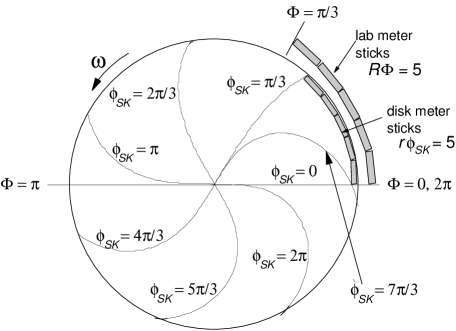
Figure 10: . Selleri-Klauber Hybrid Coordinates

Further, the 4D physical component in rotation is

$$\sqrt{1-\omega^{2}r^{2}/c^{2}}rd\phi_{SK}=\,\mbox{meters}\,\mbox{for}\,\mbox{the}\,\mbox{interval}\,\,ds\,\mbox{in}\,\mbox{rotating}\,\mbox{frame}\,\mbox{coords}.$$ (52)

This, of course, equals ds in the lab between the same two events, which equals (51), i.e.,

$$Rd\Phi=\,\mbox{meters}\,\mbox{for}\,\mbox{same}\,\mbox{interval}\,\,ds\,\mbox{in}\,\mbox{lab}\,\mbox{coords}.$$ (53)

13.2.2 The transformation and the metric

Relationship (50), for a local Selleri type $x-y-z$ spatial grid, equals what Selleri calls (with our notation of Secs. 8.1 and 9.2.2) dx_S, and what we have called dx_K, the alternative Klauber approach (Sec. 9.2.2). Thus,

$$rd\phi_{SK}=dx_{S}=dx_{K}.$$ (54)

However, this $x-y-z$ grid approach (middle and right parts of (54)) is limited to local frames, and does not yield a global rotating frame metric. To yield a fully functional general relativistic approach, we switch to a transformation and metric expressed in 1) global cylindrical coordinates, and 2) judiciously chosen coordinates, such that $t_{SK}$ and rd$\phi$_SK equal time measured on standard clocks, and length measured with standard meter sticks, respectively.

Thus, the transformation from lab (upper case) to rotating frame (lower case) coordinates is a hybrid of the Selleri and Klauber transformations, i.e.,

$$\begin{array}[]{c}ct_{SK}=\sqrt{1-\omega^{2}r^{2}/c^{2}}cT\quad\quad\quad\quad\quad\mbox{(a)}\\ r=R\quad\quad\quad\quad\quad\quad\;\;\;\quad\,\,\,\,\,\,\,\,\,\,\,\,\,\,\,\,\,\,\,\,\,\,\,\,\,\,\mbox{(b)}\\ \phi_{SK}=\frac{1}{\sqrt{1-\omega^{2}r^{2}/c^{2}}}\left({\Phi-\omega T}\right)\quad\;\,\,\,\,\,\,\mbox{(c)}\\ z=Z\quad\quad\quad\quad\quad\quad\quad\;\;\;\,\,\,\,\,\,\,\,\,\,\,\,\,\,\,\,\,\,\,\,\,\,\,\,\,\,\,\mbox{(d)}\\ \end{array},$$ (55)

where we have used subscripts only on those coordinates that vary from their lab counterparts (and that differ from either the original Selleri or Klauber approaches).

The inverse transformation of (55) is

$$\begin{array}[]{c}cT=\frac{ct_{SK}}{\sqrt{1-\omega^{2}r^{2}/c^{2}}}\quad\quad\quad\quad\quad\quad\quad\quad\,\,\,\,\,\,\,\mbox{(a)}\\ R=r\quad\quad\quad\quad\quad\quad\quad\;\;\;\quad\,\,\,\,\,\,\,\,\,\,\,\,\,\,\,\,\,\,\,\,\,\,\,\,\,\,\,\,\,\,\,\mbox{(b)}\\ \Phi=\sqrt{1-\omega^{2}r^{2}/c^{2}}\phi_{SK}+\frac{\omega t_{SK}}{\sqrt{1-\omega^{2}r^{2}/c^{2}}}\quad\;\,\mbox{(c)}\\ Z=z\quad\quad\quad\quad\quad\quad\quad\quad\;\;\;\,\,\,\,\,\,\,\,\,\,\,\,\,\,\,\,\,\,\,\,\,\,\,\,\,\,\,\,\,\,\,\,\mbox{(d)}\,\mbox{.}\\ \end{array}$$ (56)

We need to express (56) in differential form, since by substituting into the lab line element, we can find the rotating frame line element, and thus, the rotating frame metric. Thus, we find

$$\begin{array}[]{c}cdT=\frac{cdt_{SK}}{\sqrt{1-\omega^{2}r^{2}/c^{2}}}\,\,-\,\,\frac{t_{SK}}{\left({1-\omega^{2}r^{2}/c^{2}}\right)^{3/2}}\left({\frac{\omega^{2}r}{c^{2}}}\right)dr\quad\quad\quad\quad\,\,\,\,\,\,\,\mbox{(a)}\\ dR=dr\quad\quad\quad\quad\quad\quad\quad\;\;\;\quad\quad\quad\quad\quad\quad\quad\,\,\,\,\,\,\,\,\,\,\,\,\,\,\,\,\,\,\,\,\,\,\,\,\,\,\,\,\,\,\,\,\,\,\,\mbox{(b)}\\ d\Phi=\sqrt{1-\omega^{2}r^{2}/c^{2}}d\phi_{SK}-\,\,\frac{\phi_{SK}}{\left({1-\omega^{2}r^{2}/c^{2}}\right)^{3/2}}\left({\frac{\omega^{2}r}{c^{2}}}\right)dr\\ \,\,\,\,\,\,\,\,\,\,+\frac{\omega dt_{SK}}{\sqrt{1-\omega^{2}r^{2}/c^{2}}}+\frac{\omega t_{SK}}{\left({1-\omega^{2}r^{2}/c^{2}}\right)^{3/2}}\left({\frac{\omega^{2}r}{c^{2}}}\right)dr\quad\quad\quad\quad\;\,\,\,\,\,\,\,\,\,\,\,\,\mbox{(c)}\\ dZ=dz\quad\quad\quad\quad\quad\quad\quad\quad\quad\quad\quad\quad\quad\quad\quad\;\;\;\,\,\,\,\,\,\,\,\,\,\,\,\,\,\,\,\,\,\,\,\,\,\,\,\,\,\,\,\,\,\,\,\,\,\,\mbox{(d)}\,\mbox{.}\\ \end{array}$$ (57)

Substituting, along with $R=r$, into

$$(ds)^{2}=-(cdT)^{2}+(dR)^{2}+(Rd\Phi)^{2}+(dZ)^{2},$$ (58)

one gets a very complicated line element and resulting metric, with the latter having many off diagonal terms. From the non-orthogonality between lines of constant $\phi$_SK and $r$ seen in Fig. 10, the drd$\phi$ terms are to be expected. With a little thought, the other terms make sense as well.

We will not carry out the tedium of constructing the metric, but it is straightforward, and can be used to solve virtually any problem in rotation. Since the coordinate values dt_SK and d$\phi$_SK (via rd$\phi$${}_{SK})$ reflect the real world measured values, components of vectors and tensors will directly equal the real world values (provided, for example, that one multiplies contravariant components in the $\phi$_SK direction by $r$.)

We will do something a little simpler, computation-wise, by considering dr = dz = 0, i.e., motion along a circumferential line. For this case, (58) and (57) yield the line element

$$(ds)^{2}=-(cdt_{SK})^{2}+r^{2}\left({1-\omega^{2}r^{2}/c^{2}}\right)(d\phi_{SK})^{2}+2r^{2}\omega d\phi_{SK}dt_{SK}.$$ (59)

Considering light with ds = 0, and using the quadratic equation formula to solve (59) for the one-way speed of light rd$\phi$_SK/dt_SK, we find

$$v_{real\,world,\mbox{ }circum,\mbox{ }1-way}=\frac{rd\phi_{SK}}{dt_{SK}}=\frac{\omega r\pm c}{1-\omega^{2}r^{2}/c^{2}},$$ (60)

where the sign in the numerator before $c$ indicates the direction of the light ray, ccw or cw.

Using (60), one can find the back and forth, MM time to be

$$t_{MM}=\frac{l}{\left|{v_{+}}\right|}+\frac{l}{\left|{v_{-}}\right|}=\frac{2l}{c},$$ (61)

and thus, the back and forth speed of light along the circumference is $c$.

Similarly the Sagnac time difference for cw and ccw rays, with $l=2\pi r/\sqrt{1-\omega^{2}r^{2}/c^{2}}$, is

$$t_{Sagnac,\,real\,world}=\frac{l}{\left|{v_{-}}\right|}-\frac{l}{\left|{v_{+}}\right|}=\frac{4\pi\omega r^{2}}{c^{2}\sqrt{1-\omega^{2}r^{2}/c^{2}}},$$ (62)

in agreement with (4).

For other, more general problems, due to the complicated nature of the metric found from (57) and (58), the modified Klauber approach appears far simpler computationally. As but one example, the Coriolis calculation for both approaches will be the same, but the modified Klauber method is far easier.

14 Loose Ends

14.1 Curvature: Meter Stick Measurement or Spacetime Path?

The conclusions of the prior section lead to an interesting result with regard to curvature of a rotating disk surface. Using meter stick measurements of the circumference, one would then find

$$\mbox{circumference}\,\,>2\pi r\,\,\,\,\,\left({\mbox{measured}\,\mbox{with}\,\mbox{disk}\,\mbox{meter}\,\mbox{sticks = }\Delta x_{s}}\right)$$ (63)

and thus would be inclined to deem the surface curved.

However, curvature in differential geometry is defined via the variation in the interval ds, not the coordinate value dx_S. For this, and continuous, single-valued time (such as that of the Selleri and Klauber approaches, which lead to correct Coriolis acceleration), we would have

$$\mbox{circumference}\,\,=2\pi r\,\,\,\,\,\left({\mbox{spacetime}\,\,\mbox{interval}\,\,\Delta s}\right).$$ (64)

The curvature found from the Riemann tensor is based on ds variation, not dx_S variation. Thus, Riemann curvature for the 2D disk surface is zero.

Another way to the same conclusion is to recognize that (56) with $t_{SK}$ = $z$ = 0 is simply a transformation from the 2D lab surface to the 2D rotating surface, and since the Riemann tensor for this surface is zero in the lab, it must also be zero for the rotating surface.

Conclusion: For continuous, single-valued time (i.e., correct Coriolis acceleration), the Riemann curvature for the rotating disk surface is zero, even if real world, rotating frame meter stick measurement of the circumference does not equal 2$\pi r$.

14.2 Resolution of the Limit Paradox

The Selleri limit paradox was re-cast in Sec. 2.2.2 to the following.

Given that (in order to predict correct Coriolis acceleration) time in the rotating frame must be continuous, then only a single simultaneity is allowed in that frame. Yet at Selleri’s limit, the LCIF, which is a translating frame, can have any of an infinite number of allowable simultaneity schemes, and thus is not equivalent locally to the rotating frame at that location.

As discussed in Ref. [44], the potential – $\raise 2.15277pt\hbox{$\scriptstyle 1$}\kern-1.00006pt/\kern-1.49994pt\lower 1.07639pt\hbox{$\scriptstyle 2$}\omega^{2}r^{2}$ does not go to zero in the Selleri limit, and relativistic mass depends on total energy, kinetic plus potential. Hence, in the rotating frame at the Selleri limit, mass of a proton, for example, would be different than the mass of a proton in the LCIF. Thus, by simply measuring the mass of Avogadro’s number of carbon atoms, for example, in each frame, one could discern which of the two were rotating. Thus, they are not equivalent.

Conclusion: Change in mass, due to potential energy, in a rotating frame permits one to distinguish between that frame and an LCIF frame.

15 Summary of Conclusions

The most important result of this article is that correct Newtonian limit Coriolis acceleration can only be predicted by general relativity for a unique simultaneity in the rotating frame, where this simultaneity equals that of the lab and ensures continuity of time (single valued time, with clocks in synchronization with themselves.) I submit this settles what has probably been the most contentious issue in relativistic rotation. We list this conclusion with others below.

15.1 Lorentz Contraction

• The widely dispersed logic justifying circumferential Lorentz contraction in a rotating frame is submitted to contain unresolved inconsistencies.

• Contraction, by the standard definition for which end points of a meter stick are simultaneous, varies with choice of synchronization scheme, so Lorentz contraction (by the specific Lorentz factor $\gamma$) and conventionality of synchronization in rotation cannot both be true.

• Proof for Lorentz contraction in rotation was found in both the Antonini et al and Herrmann et al experiments, which conflicted with an earlier anomalous signal found by Brillet and Hall.

• The rotating disk surface has a circumference, as measured by real world meter sticks greater than 2$\pi r$, but an interval $\Delta s$ equal to 2$\pi r$, and thus its 2D Riemann curvature is zero.

15.2 Simultaneity/Synchronization

• Coriolis acceleration arises in the general relativistic equation of motion from the off diagonal time-space term in the metric. This term is dependent upon choice of simultaneity.

• Correct Newtonian limit Coriolis acceleration only arises from one simultaneity choice, the one for which time is continuous (and clocks are in synchronization with themselves), and thus, there is no conventionality of synchronization in rotation.

15.3 Locality and the Selleri Limit “Paradox”

• Due to relativistic mass changes from potential energy, the rotating frame is not locally equivalent to a LCIF.

• The newly formulated version of the Selleri limit “paradox” is thus resolved, as the LCIF and rotating frames in the limit are not equivalent.

15.4 Comparison of Theories

• The traditional LCIF approach to rotation, in its most modern version, the RRS approach, embraces conventionality of synchronization and thus, for reasons delineated herein, is argued to be incorrect. Further, it provides no global metric and therefore is incapable of being a generally applicable approach to all problems in rotation, such as, for one example, Coriolis acceleration.

• The original Selleri approach has the correct simultaneity and agrees with the Antonini et al, Herrmann et al, and Sagnac experiments. However, it does not provide a global metric, and thus is also not fully applicable to general problems.

• Bel’s approach predicts a non-null MM result and thus disagrees with the recent experiments. Further, his theory appears to be in conflict with the Byl et al experiment.

• Nikolic predicts the correct Newtonian Coriolis acceleration and a null MM signal, but his global (i.e. integrated) time appears discontinuous, and he provides no global metric. Further, his argument that there is no single rotating frame, but only an infinite series of local frames, appears difficult to justify.

• Klauber has continuous time and the correct Coriolis acceleration, but disagrees with the Antonini et al and Herrmann et al experiments. His prediction of no rotational Lorentz contraction (based on an interpretation of the standard physical component analysis method of differential geometry) is almost certainly incorrect.

• None of the proposed theories of rotation makes correct predictions for all cases.

15.5 Two Suitable Theories of Rotation

• A modified Klauber theory, for which contravariant physical components in the circumferential direction are modified by the Lorentz factor is simple, generally applicable to rotation, and provides the correct results for all cases.

• A hybrid Selleri-Klauber theory, in which Selleri’s “built-in” Lorentz contraction is incorporated by selecting one particular spatial coordinate grid, provides the correct simultaneity, as well as a global metric with the capability of analyzing all problems.

16 Acknowledgements

I thank two anonymous reviewers for suggesting changes that markedly clarified the presentations of several sections.

References

- [1] G. Rizzi and M.L. Ruggiero, Ed., Relativity in Rotating Frames (Kluwer Academic, Dordrecht, The Netherlands, 2004) http://digilander/libero.it/solciclos/
- [2] G. Rizzi, M.L. Ruggiero, and A. Serafini, “Synchronization gauges and the principles of special relativity,” Found. Phys. 34(12), 1835-1887 (Dec 2004).
- [3] F. Selleri, “The inertial transformations and the relativity principle,” Found. Phys. Lett. (18)4, 325-339 (Aug 2005).
- [4] P. Antonini, M. Okhapkin, E. Göklü, and S. Schiller, “Test of constancy of speed of light with rotating cryogenic optical resonators,” Phys. Rev. A 71, 050101 (2005). gr-qc/0504109
- [5] P.L. Stanwix et al, “Test of Lorentz invariance in electrodynamics using rotating cryogenic sapphire microwave oscillators,” Phys. Rev. Lett. 95, 040404 (2005). hep-ph/0506074.
- [6] S. Herrmann et al, “Test of the isotropy of the speed of light using a continuously rotating optical resonator,” Phys. Rev. Lett. 95, 150401 (2005). physics/0508097.
- [7] C. Møller, The Theory of Relativity, (Clarendon Press, Oxford, 1969), pp. 223.
- [8] J. Stachel, ”Einstein and the rigidly rotating disk,” Chapter 1 in Held, General Relativity and Gravitation (Plenum Press, New York, 1980), p. 9; A. Einstein, The Meaning of Relativity (Princeton University Press, 1950), footnote on pg 60.
- [9] B. Mashoon, “Gravitation and nonlocality,” gr-qc/0112058; “The hypothesis of locality and its limitations,” Chapter 3 in Ref [1].
- [10] Ref. [8], p. 7.
- [11] Ø. Grøn, ”Relativistic description of a rotating disk,” Am. J. Phys. 43(10), 869-876 (1975). Grøn’s treatment has become a classic for traditional approach advocates.
- [12] Ø. Grøn, ”Rotating frames in special relativity analyzed in light of a recent article by M. Strauss,” Int. J. Theor. Phys. 16(8), 603-614 (1977).
- [13] Ø. Grøn, “Space geometry in rotating frames: A Historical Perspective,” Chapter 15 in Ref [1].
- [14] T.A. Weber, Response to “Comments regarding recent articles on relativistically rotating frames,” Am. J. Phys. 67(2), 159-160 (Feb 1999).
- [15] T.A. Weber, “Measurements on a rotating frame in relativity, and the Wilson and Wilson experiment,” Am. J. Phys. 65(10), 946-953 (Oct 1997).
- [16] R.D. Klauber, “Toward a consistent theory of relativistic rotation,” Chapter 6 in Ref [1]. physics/0404027
- [17] G. Rizzi, and A. Tartaglia, “On local and global measurements of the speed of light on rotating platforms,” Found. Phys. Lett. 12(2), 179-186 (April 1999).
- [18] G. Rizzi, and M.L. Ruggiero, “Space geometry of rotating platforms: an operational approach,” Found. Phys. 32, 1525 (2002). gr-qc/0207104.
- [19] G. Rizzi, and A. Serafini, “Synchronization and desynchronization on rotating platforms,” Chapter 5 in Ref [1].
- [20] M.B. Cranor, E.M. Heider, R.H. Price, “A circular twin paradox,” Am. J. Phys. 68(11), 1016-1020 (Nov 2000).
- [21] J. Anandan, “Sagnac effect in relativistic and nonrelativistic physics,” Phys. Rev. D 24(2), 338-346 (15 July 1981).
- [22] S.K. Ghosal, B. Raychaudhuri, A.K. Chowdhury, and M. Sarker, “On the anisotropy of the speed of light on a rotating platform,” Found. Phys. Lett. 17, 457 (2004).
- [23] A. Peres, “Synchronization of clocks in a rotating frame,” Phys. Rev. D. 18(6), 2173-2174 (15 Sept 78).
- [24] D. Dieks, “Time in special relativity and its philosophical significance,” Eur. J. Phys. 12, 253-259 (1991).
- [25] R. Anderson, I. Vetharaniam, G.E. Stedman, “Conventionality of synchronisation, gauge dependence and test theories of relativity,” Phys. Rep. 295(3&4), 93-180 (March 1998). Many articles have appeared on this subject. These authors cite virtually all of them prior to 1998.
- [26] F. Selleri, “Sagnac effect: end of the mystery,” Chapter 4 in Ref [1].
- [27] F. Selleri, “Noninvariant one-way speed of light and locally equivalent reference frames,” Found. Phys. Lett. 10, 73-83 (1997).
- [28] M. G. Sagnac, Comptes Rendus 157, 708-718 (1913); “Effet tourbillonnaire optique. La circulation de l’éther lumineux dans un interférographe tournant,” Journal de Physique Thèorique et Appliqèe Paris, Sociète française de physique, Series 5, 4, (1914), 177-195.
- [29] E.J. Post, ”Sagnac effect,” Rev. Mod. Phys. 39, 475-493 (1967).
- [30] Ref. [19], pp. 98-99, also Ref. [1], p. 409.
- [31] F. Selleri, “Curing one discontinuity with another: Comment on S.K. Ghosal et al,” Found. Phys. Lett. 17, 599-606 (2004).
- [32] R.D. Klauber, “Non-time-orthogonality, gravitational orbits and Thomas precession,” gr-qc/0007018.
- [33] A. Tartaglia, “Lengths on rotating platforms,” Founds. Phys. Lett. 12(1), 17-28 (1999).
- [34] M. Strauss, ”Rotating frames in special relativity,” Intl. J. Theor. Phys. 11, 107-123 (1974).
- [35] R. D. Klauber, “Derivation of the general case Sagnac experimental result using NTO analysis,” Found. Phys. Lett. 16(5), 441-457 (Oct 2003). gr-qc/0206033.
- [36] See extensive discussions in Ref. [1].
- [37] M. Born, Einstein’s Theory of Relativity (Dover, NY, 1965) pp. 214-216.
- [38] A. Brillet and J. L. Hall, “Improved laser test of the isotropy of space,” Phys. Rev. Lett. 42(9), 549-552 (1979).
- [39] L. Bel, “Eppur, si muove!” Chapter 12 in Ref [1].
- [40] R.D. Klauber, “Analysis of the anomalous Brillet and Hall experimental result,” Found. Phys. Lett. 17(2), 125-147 (April 2004).
- [41] The texts and articles listed below are among those that discuss physical vector and tensor components. Ref. [16], pp. 114-116; D. Savickas, “Relations between Newtonian Mechanics, general relativity, and quantum mechanics,” Am. J. Phys. 70, (8), 798-806; I.S. Sokolnikoff, Tensor Analysis, (Wiley & Sons, NY, 1951) pp. 8, 122-127, 205; G.E. Hay, Vector and Tensor Analysis (Dover, 1953) pp 184-186; A.J. McConnell, Application of Tensor Analysis, (Dover, 1947) pp. 303-311; C.E. Pearson, Handbook of Applied Mathematics, (Van Nostrand Reinhold, 1983 2nd ed.), pp. 214-216; M.R. Spiegel, Schaum’s Outline of Vector Analysis (Schaum) p. 172; R.C. Wrede, Introduction to Vector and Tensor Analysis, (Dover, 1972), pp. 234-235.
- [42] C.W. Misner, K.S. Thorne, and J.A. Wheeler, Gravitation (Freeman, NY, 1973) p. 210.
- [43] See Sec. 2.5.2 of Ref. [25] for further discussion and citations of prior work on this topic.
- [44] R.D. Klauber, “New perspectives on the relativistically rotating disk and non-time-orthogonal reference frames,” Found. Phys. Lett. 11(5), 405-443. qc-gr/0103076. See Sec. 4.1. These relations can be found elsewhere as well.
- [45] L. Bel, J. Martin, and A. Molina, “Rigid motion in special and general relativity,” Jour. Phys. Soc. Japan 63(12), 4350-4363 (Dec 94).
- [46] L. Bel, and A. Molina, “Local anisotropy of space in a frame of reference co-moving with the Earth,” Il Nuovo Cimento 11B(6) (2000) and arXiv: gr-qc/9806099.
- [47] Ref. [1], contributions to Dialogues III and IV, pp. 411-437.
- [48] Ref. [1], p. 433.
- [49] J. Byl, M. Sanderse, W. van der Kamp, “Simple first-order test of special relativity,” Am. J. Phys. 53(1), 43-45 (Jan 85).
- [50] H. Nikolic, “Proper co-Ordinates of non-inertial observers and rotation,” Chapter 14 in Ref [1].
- [51] Ref [50], p. 278.
- [52] R.D. Klauber, “Non-time-orthogonality and tests of special relativity,” gr-qc/0006023 (June 2000)
- [53] R.D. Klauber, “Generalized tensor analysis method applied to non-time-orthogonal coordinate frames,” gr-qc/0107035 (July 2001).