Ultrarelativistic sources in nonlinear electrodynamics

Abstract

The fields of rapidly moving sources are studied within nonlinear electrodynamics by boosting the fields of sources at rest. As a consequence of the ultrarelativistic limit the $\delta$–like electromagnetic shock waves are found. The character of the field within the shock depends on the theory of nonlinear electrodynamics considered. In particular, we obtain the field of an ultrarelativistic charge in the Born–Infeld theory.
Keywords: nonlinear electrodynamics, ultrarelativistic limit, Born–Infeld theory
PACS numbers: 03.50.Kk, 04.40.Nr, 11.10.Lm

1 Introduction

It was realized a long time ago within Maxwell’s theory that the electromagnetic field of a uniformly moving charged particle with velocity $\beta$ approaching velocity of light $(c=1)$ is approximately the same as the field of a pulse of a plane wave. This similarity was exploited in the studies of the electromagnetic interactions of relativistic particles by Fermi, Weizsa̋cker, Williams and others—see, e.g., [1] for a brief review. A rigorous treatment of the limiting field arising when $\beta=1$ was studied much later—after the spacetime representing a Schwarzschild black hole boosted to the velocity of light was found [2], and ultrarelativistic limits proved to be of a great value also in general relativity and other gravity theories. The limiting fields have been used as ‘incoming states’ in the scattering processes with high initial speeds, including the quantum scattering of two pointlike particles at center–of–mass energies higher or equal to the Planck energy. This quantum process has been shown to have close connection with classical black hole collisions at the speed of light—see, e.g., [3], [4], [5], [6].

A careful study of the ultrarelativistic limits—or so–called ‘lightlike contractions’—of electromagnetic fields in Minkowski space within Maxwell’s theory was done in 1984 by Robinson and Rózga [7]. They considered lightlike contractions of general multipole fields and have established, as expected, that the field gets concentrated on null hyperplanes where it shows the $\delta$–like profile, and resembles a plane wave. The multipole structure of higher order than monopole can be preserved in such a limit. All these fields possess pointlike singularities travelling with the speed of light. They survive the lightlike contractions. A ‘lightlike singularity’ is present also in the Aichelburg–Sexl metric arising from the lightlike contraction of a family of Schwarzschild spacetimes [2, 8].

In this paper we study the ultrarelativistic limits in the theories of nonlinear electrodynamics (NLE) which represent models of classical singularity–free theories with acceptable concepts of point charges (see, e.g., [9], [10] for a review). Nonlinear electromagnetic effects in vacuum are under investigation by experimentalists (e.g. [11]), however, Maxwell’s theory and quantum electrodynamics are in a remarkably good agreement with an experiment until now. Our motivation stems from a basic question whether, and if yes then how, finiteness of the fields of static charges in a suitable NLE survives the ultrarelativistic limit, and also from the interest in NLE, most notably in the Born-Infeld (BI) theory [12], which arose relatively recently owing to the developments in string theories (see, e.g., [13]). In these theories the BI theory appears as an effective theory at different levels [14], especially in connection with $p$–branes [15]. For example the motion of a single isolated $(p+1)$–dimensional D–brane moving in a flat $(d+1)$–dimensional spacetime is governed by so–called Dirac–Born–Infeld action

$$S_{\rm DBI}=\int\!d^{p+1}x\sqrt{-{\rm det}(G_{\mu\nu}+2\pi\alpha^{\prime}F_{\mu\nu})},\quad G_{\mu\nu}=\eta_{mn}\frac{\partial z^{m}}{\partial x^{\mu}}\frac{\partial z^{n}}{\partial x^{\nu}},$$ (1)

where $m,n=0,...d,\ \mu,\nu=0,...p$, $G_{\mu\nu}$ is Minkowskian metric induced on D–brane, $F_{\mu\nu}=\partial_{\mu}A_{\nu}-\partial_{\nu}A_{\mu}$, and $\alpha^{\prime}$ is the inverse string tension. In ‘Monge gauge’ the vector field $A_{\mu}$ directly satisfies the Born–Infeld field equations in $(p+1)$–dimensional spacetime [16].

Even at classical level the position of the BI theory among other NLEs is exceptional. As some other NLEs it yields finite static fields with finite energy. However, it is the only NLE in which the speed of light does not depend on the polarization, i.e. no birefringence phenomena occurs [10, 17]. The BI system of equations can be enlarged as a system of hyperbolic conservation laws with remarkable properties which recently attracted attention (see [18] and references therein).

Our paper is organized as follows: In the next section the concept of ultrarelativistic limit is revised. In the third section a spherically symmetric solution of NLE is summarized. The main results are formulated in the Section 4 where the procedure how to find the ultrarelativistic fields of a charge coupled to an arbitrary NLE is presented and consequently applied on the Born–Infeld charge (BIon [16]). Finally follow the concluding remarks.

2 The ultrarelativistic limit

Following closely [7], [8], we first briefly describe what we mean by the ultrarelativistic limit of the electromagnetic fields in mathematical terms. Denote by $(M,{\bf g})$ Minkowski space, with a chart $X:M\,\rightarrow\,\mathbb{R}^{4}$ with coordinates $x^{\mu}$ in which $g_{\mu\nu}=\eta_{\mu\nu}$ is a Lorentzian metric. Next, consider Lorentz boosts $\Phi_{\beta}:M\,\rightarrow\,M,\;|{\beta}|<1$, characterized by charts $X_{(\beta)}:M\ \rightarrow\ {\bf R}^{4}$ with coordinates $x_{(\beta)}^{\mu}$, i.e., $x^{\mu}=\Lambda^{\ \ \ \mu}_{(\beta)\ \;\nu}x^{\nu}_{(\beta)}$. For an arbitrary tensor field ${\bf T}$ on $M$, the motions $\Phi_{\beta}$ induce one–parameter family of the fields $\star\Phi_{\beta}{\bf T}$ on $M$, where $\star\Phi$ is ‘derivative of $\Phi$’ (see e.g. [19], Appendix C). If an electromagnetic field tensor ${\bf F}$ is given on $M$, $\star\Phi_{\beta}{\bf F}$ denotes the corresponding family of ‘boosted’ electromagnetic fields; we also have $\star\Phi_{\beta}{\bf g}={\bf g}$. We understand the ultrarelativistic—or lightlike—limit as a distributional limit $|\beta|\to 1$ of this family.

In the case of linear theories one can prove, using the theory of distributions, that the ultrarelativistic limit ‘commutes with field equations’, i.e., the fields after the limit satisfy again the field equations. With nonlinear theories one could turn to Colombeau theory [20], which provides a possible framework for studying nonlinear operations with singular functions. However, we do not attempt this here—in fact, we do not need to do it. In the following we shall see that in case of nonlinear electrodynamics the fields obtained by the ultrarelativistic limit are well behaved functions within distribution theory.

Let us conclude this section by quoting two mathematical lemmas which will be needed in Section 4 (for proofs see [21], [22]):
Lemma 1. Let $h\geq 0$ is a Lebesgue integrable function in $\mathbb{R}$ and $\int\!h(x)dx=1.$ Then $\lim\limits_{A\to 0}\frac{1}{A}h\!\left(\frac{x}{A}\right)\stackrel{{\scriptstyle D^{\prime}}}{{=}}\delta(x)$, where $D^{\prime}$ denotes the limit in a distributional sense.
Lemma 2. Let $\alpha_{\lambda}$ is a sequence of smooth ($C^{\infty}$) functions on a compact region $\Omega\subset\mathbb{R}^{n}$, which converge uniformly to a smooth function $\alpha$, and the same is true for all their derivatives. Let a sequence of distributions $g_{\lambda}$ converges to a distribution $g$, $g_{\lambda}\!\stackrel{{\scriptstyle D^{\prime}(\Omega)}}{{\longrightarrow}}g$. Then $\alpha_{\lambda}g_{\lambda}\stackrel{{\scriptstyle D^{\prime}(\Omega)}}{{\,\longrightarrow\,}}\alpha g$. If furthermore $\left(\partial_{1}\alpha_{(\lambda)}(x)\right)^{2}+\dots+\left(\partial_{n}\alpha_{(\lambda)}(x)\right)^{2}\nolinebreak\neq 0$, then $g_{\lambda}(\alpha_{\lambda})\stackrel{{\scriptstyle D^{\prime}(\Omega)}}{{\longrightarrow}}g(\alpha).$

3 Spherically symmetric solutions

Let $F_{\mu\nu}$ is the electromagnetic field tensor, $F_{\mu\nu}=\partial_{\mu}A_{\nu}-\partial_{\nu}A_{\mu}$. The theories of nonlinear electrodynamics start out from the Lagrangian density $\pounds$, which is an arbitrary function of the invariant $F=\frac{1}{4}\,F_{\mu\nu}F^{\mu\nu}$ and of the square of the pseudoinvariant $G=\frac{1}{4}\,F_{\mu\nu}{\,}^{\star}\!{F^{\mu\nu}}$, $\pounds=\pounds(F,G^{2}).$ Since a nonlinear behavior may prove significant only in very strong fields, one commonly requires the principle of correspondence (POC): in a weak–field limit NLEs have to approach the linear Maxwell theory that is so well experimentally confirmed. The action of NLE describing charge $Q$ interacting with electromagnetic field reads

$$S=-Q\!\int\!A_{\mu}(z)dz^{\mu}+\frac{1}{4\pi}\int\!d^{4}x\sqrt{-g}\pounds(F,G^{2}),$$ (2)

where, following POC, we impose the condition

$$\quad\lim\limits_{F^{\mu\nu}\to\,0}\pounds=F+O(F^{2},G^{2}).$$ (3)

The resulting field equations have the form

$$\left(\pounds_{,F}F^{\mu\nu}+\pounds_{,G}{\,}^{\star}\!{F^{\mu\nu}}\right)_{;\,\nu}=4\pi\frac{Q}{\sqrt{-g}}\int\!dz^{\mu}\delta(x-z).$$ (4)

Equations (2) and (4) are written in a general covariant form, $g={\rm det}\,g_{\mu\nu}$, semicolon denotes covariant derivative, $\pounds_{,F}=\partial\pounds/\partial F$, etc.

One can show that spherically symmetric solutions of (4) must necessarily be static [23]. In spherical coordinates $(t,r,\theta,\varphi)$ one finds

$$\mbox{{\bf F}}=-Edt\land dr,$$ (5)

where the radial component of the electric field $E(r)$ is implicitly given by the relation

$$\pounds_{,F}(F,G)E=\frac{Q}{r^{2}},\quad F=-\frac{1}{2}\,E^{2},\quad G=0.$$ (6)

In particular, for the Born–Infeld theory the Lagrangian density $\pounds_{\rm BI}$ and the spherically symmetric solution (5) read

$$\pounds_{\rm BI}=b^{2}\left(\sqrt{1+\frac{2F}{b^{2}}-\frac{G^{2}}{b^{4}}}-1\right),\qquad E_{\rm BI}=\frac{Q}{\sqrt{r^{4}+r_{0}^{4}}}\ \mbox{,}\quad r_{0}=\sqrt{\frac{Q}{b}};$$ (7)

here parameter $b$ plays the role of a limiting field value. The Maxwell theory is recovered in the weak field limit, $b\to\infty$. The spherically symmetric solution (7) is finite everywhere, though at the origin the electric field ceases to be smooth. It yields a finite energy.

4 Ultrarelativistic charges in nonlinear electrodynamics

We first transform the spherically symmetric solutions (5) into cylindrical coordinates $(t,z,\rho,\varphi)$ and then apply the Lorentz boost along the negative $z$–axis,

$$z=\gamma(Z+\beta T),\quad t=\gamma(T+\beta Z),\qquad\gamma=\frac{1}{\sqrt{1-\beta^{2}}}.$$ (8)

The resulting field in the boosted frame $(T,Z,\rho,\varphi)$ turns out to have the form

$$\star\Phi_{\beta}\mbox{{\bf F}}=-E^{Z}dT\land dZ-E^{\rho}dT\land d\rho-B^{\varphi}dZ\land d\rho,$$ (9)

with components

$$E^{Z}=\frac{\gamma W_{\!\beta}}{r^{\prime}}\,E(r^{\prime}),\quad E^{\rho}=\frac{\gamma\rho}{r^{\prime}}\,E(r^{\prime}),\quad B^{\varphi}=\beta E^{\rho},$$ (10)

where

$$r^{\prime}=\sqrt{\gamma^{2}W_{\!\beta}^{2}+\rho^{2}},\quad W_{\!\beta}=Z+\beta T,$$ (11)

and $E(r^{\prime})$ is given by (6) with $r\to r^{\prime}$. This field exhibits some interesting features. It is of course time–dependent since the source is in a uniform motion with velocity $\beta$. Due to this motion a cylindrically symmetric magnetic field, $B^{\varphi}$, arises. As $\beta$ increases towards velocity of light, $E^{Z}$ becomes smaller and smaller, whereas components $E^{\rho}$ and $B^{\varphi}$ approach the same ‘$\delta$–profile’. The magnetic field becomes perpendicular to the electric field and their magnitudes become equal. The field concentrates on the null hyperplane $W_{\!\beta}\to 0$. It resembles a plane wave, nevertheless, in contrast to the wave, the invariant $F$ remains nonzero. Far from the charge the behavior of the field is very nearly the same for all NLEs; as a consequence of POC, it is of course very close to the field of the boosted charge in the Maxwell theory. However, within a characteristic radius of a particular NLE, where field equations and resulting nonlinearities differ significantly, the specific features of the NLE dominate. In Figure 1 the magnitude of electric field ${\rm E}=\sqrt{(E^{\rho})^{2}+(E^{Z})^{2}}$ of a charge at rest and a charge moving with velocity $\beta=0.9$ within the BI theory is illustrated. For comparison, see Figure 2 where the same situation is displayed within the Maxwell theory. We see that the behavior of the fields of static charges is reflected also in the relativistic speeds. Although at the position of the charge $\rm E$ diverges in the Maxwell theory, it remains finite in the BI theory. In [24], a number of other plots of boosted fields are given for several specific NLEs. Another interesting effect occurs in the very ultrarelativistic case. Now we proceed to construct this limit.

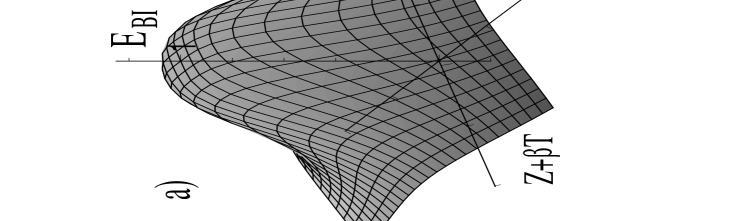
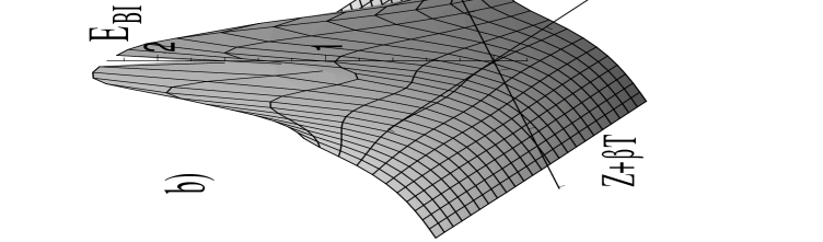
Figure 1: The magnitude of electric field in Born-Infeld theory. The graph a) displays ${\rm E}_{\rm BI}$ for a charge at rest ($\beta=0$). The graph b) displays ${\rm E}_{\rm BI}$ for a charge moving with velocity $\beta=0.9$. The units are chosen so that $Q=1$, $r_{0}=1$.

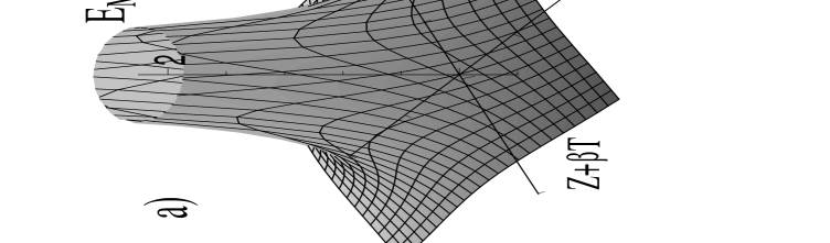
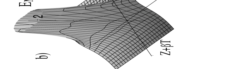
Figure 2: The magnitude of electric field in Maxwell theory. The graph a) displays ${\rm E}_{\rm M}$ for a charge at rest ($\beta=0$). The graph b) displays ${\rm E}_{\rm M}$ for a charge moving with velocity $\beta=0.9$. The figure is plotted with $Q=1$.

Let us first define function $h(y)={\rho^{2}\!E(\sqrt{y^{2}+\rho^{2}})}/(2H(\rho){\sqrt{y^{2}+\rho^{2}}})$, in which function $H$ is chosen such that $\int\!h(y)dy=1$, so that $h$ satisfies the assumptions of Lemma 1 in Section 2. Using then both Lemma 1 and 2, and putting $\gamma=1/A$, we can derive the component $E^{\rho}$ (resp. $B^{\varphi}$):

$$\lim_{\beta\to 1-}\!\!E^{\rho}=\frac{2}{\rho}\,H(\rho)\lim_{\beta\to 1-}\frac{1}{A}\,h\!\left(\frac{W_{\!\beta}}{A}\right)\ \stackrel{{\scriptstyle(L1,L2)}}{{=}}\ \frac{2}{\rho}\,H(\rho)\delta(Z+T).$$ (12)

Regarding $E^{Z}$ one can prove that this component converges pointwise to zero which implies the same convergence in the distributional sense. (For the proof, see [24].) Here we proceed in an alternative way as follows:

$$\lim_{\beta\to 1-}\!\!E^{Z}=\lim_{\beta\to 1-}\frac{W_{\!\beta}}{\rho}\,E^{\rho}\ \stackrel{{\scriptstyle(L1,L2)}}{{=}}\ \frac{2}{\rho^{2}}\,H(\rho)(Z+T)\delta(Z+T)=0,$$ (13)

where we used both Lemma 1 and 2, and standard relation $x\delta(x)=0$. The results above enable us to formulate the following
Proposition. The electromagnetic field of a rapidly moving charge constructed in a nonlinear electrodynamics with action (2) is in the ultrarelativistic limit, $\beta=1$, given by

$$\mbox{\bf F}_{{\rm ultra}}=-E^{\rho}_{{\rm ultra}}dT\land d\rho-B^{\varphi}_{{\rm ultra}}dZ\land d\rho,\quad E^{\rho}_{{\rm ultra}}=B^{\varphi}_{{\rm ultra}}=\frac{2}{\rho}\,H(\rho)\delta(Z+T),$$ (14)

where function $H$ is defined by

$$H(\rho)=\frac{\rho^{2}}{2}\int_{-\infty}^{\infty}\!\!\!\!dy\,\frac{E(\sqrt{y^{2}+\rho^{2}})}{\sqrt{y^{2}+\rho^{2}}},$$ (15)

and function $E$ is implicitly determined by the relation (6).

The radial field $E$ is given only implicitly by equation (6) and, in addition, even in cases in which it can be determined explicitly it often has such a complicated form that the integral (15) can be evaluated only numerically. It is thus useful to consider asymptotic series of this field for large distances from the source. Regarding POC we assume the series to be of the form

$$E(r)=\frac{\alpha_{1}}{r^{2}}+\frac{\alpha_{2}}{r^{3}}+\dots=\!\!\sum\limits_{n=1,2\dots}\!\!\frac{\alpha_{n}}{r^{n+1}},$$ (16)

where $\alpha_{1}$ is equal to the charge $Q$ of the source and coefficients $\alpha_{2},\alpha_{3}\dots$ depend on the choice of a particular NLE. Substituting this series into the integral (15) we obtain

$$H(\rho)=\!\!\sum\limits_{k=1,2\dots}\!\left(\frac{\alpha_{2k-1}}{\rho^{2(k-1)}}\frac{2^{2(k-1)}(k-1)!^{2}}{(2k-1)!}+\frac{\alpha_{2k}}{\rho^{2k-1}}\frac{\pi(2k-1)!}{2^{2k}k!(k-1)!}\right)\!.$$ (17)

The resulting field is then given by (14) with $H(\rho)$ above. Specifically, for the Maxwell theory we have $H(\rho)=Q$, and for the asymptotic expansion of the Born–Infeld field (7) we get

$$H_{\rm BIser}(\rho)=Q\sum\limits_{k=0}^{\infty}\!\left(\begin{array}[]{c}\!\!\!-1/2\!\!\\ \!\!\!k\!\!\end{array}\right)\!\!\left(\frac{2r_{0}}{\rho}\!\right)^{4k}\!\!\!\frac{(2k)!^{2}}{(4k+1)!}=Q\!\left(\!1-\frac{4}{15}\frac{r_{0}^{4}}{\rho^{4}}+\frac{16}{105}\frac{r_{0}^{8}}{\rho^{8}}\!\right)+O\!\left(\frac{r_{0}^{12}}{\rho^{12}}\right)\!.$$ (20)

In order to find the ultrarelativistic Born–Infeld field everywhere we must evaluate the integral (15) for the exact expression $E_{\rm BI}$ given in eq. (7). After a simple substitution this integral can be written in the form

$$H_{\rm BI}(\rho)=Q\tilde{H}_{\rm BI}\left(\frac{\rho}{r_{0}}\right),\quad\tilde{H}_{\rm BI}(x)=\frac{x^{2}}{2}\int\limits_{0}^{\infty}\!dt/{\sqrt{t(t+x^{2})([t+x^{2}]^{2}+1)}}.$$ (21)

We evaluated it numerically. The resulting field (14) is, up to the factor $\delta(Z+T)$, displayed in Figure 3. Here we plot the $\rho$–components of ultrarelativistic fields obtained within the Maxwell theory, $E^{\rho}_{\rm M}(\rm ultra)$, and in the Born–Infeld theory using both the asymptotic expansion (20), $E^{\rho}_{\rm BIser}(\rm ultra)$, and the complete solution (21), $E^{\rho}_{\rm BI}(\rm ultra)$. A striking difference between the Maxwell theory and the BI electrodynamics is here clearly exhibited: the BI field becomes zero at the origin whereas the corresponding Maxwell field diverges as $E^{\rho}_{\rm M}\approx 1/\rho$. To find the behavior of the BI field as $\rho\to 0$ analytically, we consider a constant $\epsilon$, satisfying, $x^{2}\ll\epsilon\ll 1$. Then the integral (21) can be approximated by

$$\tilde{H}_{\rm BI}(x)\approx\frac{x^{2}}{2}\left(\int\limits_{0}^{\epsilon}\!\frac{dt}{\sqrt{t(t+x^{2})}}+\int\limits_{\epsilon}^{\infty}\!\frac{dt}{t\sqrt{t^{2}+1}}\right)\approx-x^{2}\lg x+O(x^{2}).$$ (22)

It is seen that the field approaches zero as $E^{\rho}_{\rm BI}\approx-\rho\lg\rho$. Comparing the exact form of the BI field with that obtained by employing the asymptotic expansion (20) we observe that they both nearly coincide for $\rho>r_{0}$ ($r_{0}=1$ in Figure 3) and approach the Maxwell field asymptotically. (This can be shown also analytically [24].) From eqs. (14), (15) or (17) examples of the ultrarelativistic fields within other NLEs can be obtained.

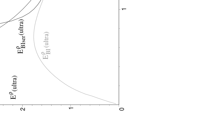
Figure 3: The field of an ultrarelativistic charge (BIon) in the BI theory. The $\rho$–components of the fields are displayed up to the factor $\delta(Z-T)$ (cf. eq. (14)). Three curves are plotted: one for the ultrarelativistic Maxwell field $E^{\rho}_{\rm M}(\rm ultra)$, and two for the Born–Infeld theory. $E_{\rm BIser}(\rm ultra)$ is constructed by using series (20), $E_{\rm BI}(\rm ultra)$ is based on the full exact solution (7), (14), (15). The units are chosen so that $Q=1$, $r_{0}=1$.

5 Concluding remarks

The properties of the ultrarelativistic fields carry the information about a theory of NLE from which they are derived. Different NLEs lead to different types of ultrarelativistic fields. For example, in the Born–Infeld theory the field remains finite but nonvanishing for all relativistic velocities $\beta$, but the field vanishes at the origin as $-\rho\lg\rho$ for the very ultrarelativistic limit. In the Hoffmann–Infeld theory [25] with the Lagrangian involving a logarithmic term the electric field vanishes at the origin for all velocities. In all cases satisfying POC at large distances the asymptotic behavior $1/r^{2}$ of the fields of uniformly moving charges changes to the ‘$1/\rho$–behavior’ in the plane moving with charge with the velocity of light in the ultrarelativistic limit.

The concept of the ultrarelativistic limit may be generalized to a curved spacetime (see, e.g., [2], [4], [6], [26]). Physically it appears plausible to perform the limit while keeping the energy of the system fixed. Then, however, one has to ‘renormalize’ the fundamental constants, e.g. mass $m\to m/\gamma$, charge $Q\to Q/\sqrt{\gamma}$; this leads to a weak field regime. In this regime the Maxwell theory appears to be fully satisfactory; the ultrarelativistic fields within the Einstein–Maxwell theory were studied in [4]. Owing to the recent interest in BI and other NLEs, several authors considered self–gravitating objects, in particular black holes, within the Einstein–NLE theories (see, e.g., [16], [27]). It would be interesting to study whether with such spacetimes ultrarelativistic limits can meaningfully be formulated while preserving the nonlinear character of the electromagnetic theory.

6 Acknowledgments

We are grateful to Professors G. W. Gibbons and V. P. Frolov for discussions. Financial support from the grand agency of the Czech Republic GAČR–202/06/0041 and Prague Centre for Theoretical Astrophysics is acknowledged.

References

- [1] J. D. Jackson, Classical Electrodynamics (John Wiley& Sons, New York, 1962, 1975, 1999).
- [2] P. C. Aichelburg and R. U. Sexl, J. Gen. Rel. Grav. 2 (1971) 303.
- [3] G. ’t Hooft, Phys. Lett. B 198 (1987) 61.
- [4] C. Loustó and N. Sánchez, Int. J. Mod. Phys. A 5 (1990) 915.
- [5] M. Fabbrichesi, R. Pettorino, G. Veneziano, and G. A. Vilkovisky, Nucl. Phys. B 419 (1994) 147.
- [6] P. D. D’Eath, Black Holes: Gravitational Interactions (Oxford University Press, Oxford, 1996).
- [7] I. Robinson and K. Rózga, J. Math. Phys. 25 (1984) 499.
- [8] P. C. Aichelburg, F. Embacher, in: Gravitation and Geometry. A volume in honour of Ivor Robinson (Bibliopolis, Naples, 1987) 21.
- [9] I. Białynicki–Birula, in: Quantum theory of particles and fields, eds. B. Jancewicz and J. Lukierski (World Scientific, Singapore, 1983).
- [10] J. Plebański, Lectures in nonlinear electrodynamics (Nordita, Copenhagen, 1970).
- [11] Frontier tests of QED and physics of the vacuum, eds. E. Zavattini, D. Bakalov, C. Rizzo (Heron Press, Sofia, 1998).
- [12] M. Born and L. Infeld, Proc. Roy. Soc. A 144 (1934) 425.
- [13] B. Zwiebach, A first course in string theory (Cambridge University Press, Cambridge, 2004).
- [14] A. A. Tseytlin and E. S. Fradkin, Nucl. Phys. B 163 (1985) 123.
- [15] L. Thorlacius, Phys. Rev. Lett. 80 (1998) 1588.
- [16] G. W. Gibbons, Nucl. Phys. B 514 (1998) 603.
- [17] G. Boillat, J. Math. Phys. 11 (1970) 941.
- [18] Y. Brenier, Arch. Rational Mech. Anal. 172 (2004) 65.
- [19] R. M. Wald, General Relativity (The University of Chicago Press, Chicago, 1984).
- [20] J. F. Colombeau, New generalized functions and multiplication of distributions (North Holland, Amsterdam, 1985).
- [21] M. A. Al–Gwaiz, Theory of distributions, ed. Dekker M. (New York, 1992).
- [22] P. Antosik, J. Mikusiński, R. Sikorski, Theory of distributions—the sequential approach (Elsevier, Amsterdam, 1973).
- [23] J. Bičák, J. Slavík, Acta Phys. Polon. B6 (1975) 489.
- [24] D. Kubizňák, MSc Thesis (The Charles University Prague, Prague, 2004).
- [25] B. Hoffmann, L. Infeld, Phys. Rev. 51 (1937) 765.
- [26] C. Barrabes, P. A. Hogan, Singular null hypersurfaces in General Relativity (World Scientific, Singapore, 2003).
- [27] E. Ayón–Beato and A. García, Phys. Rev. Lett. 80 (1998) 5056.