Kerr black hole lensing for generic observers in the strong deflection limit

Abstract

We generalize our previous work on gravitational lensing by a Kerr black hole in the strong deflection limit, removing the restriction to observers on the equatorial plane. Starting from the Schwarzschild solution and adding corrections up to the second order in the black hole spin, we perform a complete analytical study of the lens equation for relativistic images created by photons passing very close to a Kerr black hole. We find out that, to the lowest order, all observables (including shape and shift of the black hole shadow, caustic drift and size, images position and magnification) depend on the projection of the spin on a plane orthogonal to the line of sight. In order to break the degeneracy between the black hole spin and its inclination relative to the observer, it is necessary to push the expansion to higher orders. In terms of future VLBI observations, this implies that very accurate measures are needed to determine these two parameters separately.

I Introduction

As predicted by General Relativity, photons passing near a black hole suffer deviations from their original trajectory. If the minimum distance between photon and black hole is much larger than the gravitational radius, a weak field approximation of the metric tensor is sufficient to describe the light deflection. Two images of the original source are then detected by the observer. On the other hand, photons passing very close to the black hole may suffer very large deviations without falling into the black hole. These photons may perform one or more loops around the black hole before reemerging in the observer direction, thus generating two infinite sets of relativistic images very close to the black hole shadow. It can be easily intuited that these relativistic images represent a unique probe to gain information on the very strong gravitational fields surrounding the black holes. Through their study it would be possible to learn the properties of black holes and get new insight on General Relativity in a strong field regime. The features of relativistic images will thus represent a possible challenge arena for alternative theories of gravitation.

Even though a general relativity approach to this subject typically results in involved equations and heavy numerical integrations, a surprisingly simple formula for the deflection angle induced by a Schwarzschild black hole in the Strong Deflection Limit (SDL) was proposed by Darwin Dar and revived in Refs. Lum ; Oha ; BCIS . The logarithmic divergence of the deflection angle in the impact parameter was showed to be universal and valid for all spherically symmetric black holes Boz1 , as every class of such black holes leads to the same expansion for the deflection angle, with coefficients depending on the specific form of the black hole metric. The SDL method was then applied to several classes of black holes, ranging from Reissner-Nordström to black holes in string theory, from braneworld black holes to wormholes Spheric . By the SDL method it is thus possible to quantify the observables related to relativistic images for any class of spherically symmetric black holes, allowing an easy comparison among different theories. For alternative methods, see Refs. Alternative ; VirEll .

For spinning black holes, things do not work so easily. Starting from the geodesics equations in Kerr spacetime, that Carter Car reduced to first order equations depending on four constants of motion, many numerical approaches have been developed to study and visualize such geodesics. Numerical efforts have also been profused in the context of gravitational lensing to investigate the apparent shape of the accretion disk of the black hole Lum ; FMA ; Accret , the light curve of a star orbiting around it CunBar and the structure of the caustics RauBla , which turned out to be extended and to have a 4-cusped astroid structure. Some interesting general results have recently been derived through Morse theory HasPer . The extension of the SDL methodology to Kerr black holes was firstly performed in Ref. BozEq and the SDL formula was recovered for photons lying near to the equatorial plane. Anyway the expansion coefficients had to be calculated numerically as functions of the lens spin.

A first step toward a complete analytical treatment of this subject was made in Ref. BDLSS (hereafter Paper I) where the lens equation was analytically solved in the limit of small values of the angular momentum of the black hole (denoted by $a$) and for observers lying on its equatorial plane. This last assumption, besides ensuring simpler equations, was justified by the fact that the most important black hole candidate (Sgr A*, firstly suggested in Ref. VirEll ) is hosted in the center of our Galaxy and presumably has a spin-axis perpendicular to the Galactic plane, where the solar system lies. The expansions for small values of the angular momentum allowed to use the Schwarzschild SDL formula as a starting point for the description of the deflection of light rays looping around a Kerr black hole.

This analytical approach provided very simple equations (which could even be inverted for sources near to a caustic) and a full description of the extended structure of the caustics, which were confirmed to have a 4-cusped structure, symmetric w.r.t. the equatorial plane and shifted from the optical axis. Only the first order caustic cannot be recovered in the SDL approach as it is formed in the weak deflection regime RauBla ; Ser . It was also shown that the extension of relativistic caustics enhances the cross section for the creation of additional images, whose magnification is sensible in a relatively large region around the caustic. Direct observations of these relativistic images, which should be possible with the resolutions achieved by future projects, could test the Kerr nature of black hole lenses (see e.g. Refs. S1-S14 ; BDLSS for detailed discussions on observational perspectives). It is interesting to compare the lensing effect of a Kerr black hole to that of a Schwarzschild black hole embedded in an external gravitational field. Also in the latter case astroid caustics arise, though with different sizes and positions BozSer .

In this Paper we further investigate Kerr black hole lensing, getting rid of the equatorial observer hypothesis. In spite of the presence of a new parameter (the inclination of the spin axis relative to the line of sight, that we shall indicate by $\vartheta_{o}$), the surprisingly simple structure of all analytical results is preserved. Our philosophy will be to try to confine all technicalities to the appendices or refer the reader to Paper I for more detailed derivations. This paper will thus keep its main focus on the implications of all results on observable quantities. What emerges from our study is that all observables (to the lowest order) just depend on $a\sin\vartheta_{o}$, that is the projection of the spin on a plane orthogonal to the line of sight. The consequences of this fact will be discussed in the conclusions in Section 7.

Our paper is structured as follows: in Section 2 we recall the main properties of Kerr geodesics. In Section 3, we trace the borders of the shadow of the Kerr black hole for all values of the observer declination. In Section 4 we apply the SDL to null Kerr geodesics illustrating the main strategy and referring to two appendices for the details. In Section 5 we derive the critical curves and caustics structure and in Section 6 we analyze the lens mapping in the neighbourhood of a caustic, finding the position and the magnification of the images, concluding with a discussion on the detectability of relativistic images.

II Kerr geodesics

In this section, we shall review the basics of Kerr geodesics and introduce the notations to be used throughout the paper. For more details on the physical meaning of all quantities, the reader may refer to Paper I or directly to Ref. Cha .

The main subject of our paper is the Kerr black hole, whose metric in Boyer-Lindquist coordinates BoyLin , $x^{\mu}\equiv(t,x,\vartheta,\phi)$ reads

$$ds^{2}= \frac{\Delta-a^{2}\sin^{2}\vartheta}{\rho^{2}}dt^{2}-\frac{\rho^{2}}{\Delta}dx^{2}-\rho^{2}d\vartheta^{2}$$ (1)

$$-\frac{\left(x^{2}+a^{2}\right)^{2}-a^{2}\Delta\sin^{2}\vartheta}{\rho^{2}}\sin^{2}\vartheta d\phi^{2}$$

$$+\frac{2ax\sin^{2}\vartheta}{\rho^{2}}dtd\phi$$

$$\Delta= x^{2}-x+a^{2},$$ (2)

$$\rho^{2}= x^{2}+a^{2}\cos^{2}\vartheta.$$ (3)

Distances are measured in units of the Schwarzschild radius ($2MG/c^{2}=1$), $\vartheta$ and $\phi$ are the colatitude and azimuth respectively, $x$ is the radial coordinate and $a$ is the specific angular momentum of the black hole, running from $0$ (Schwarzschild black hole) to $1/2$ (extremal Kerr black hole) in our units.

We consider a static observer at Boyer-Lindquist coordinates $(D_{OL},\vartheta_{o},\phi_{o})$. The distance between observer and black hole is thus $D_{OL}$, while the colatitude $\vartheta_{o}$ of the observer coincides with the inclination of the spin on the line of sight $\overline{OL}$. Exploiting the freedom to choose the zero of the azimuth, we set $\phi_{o}=\pi$. We will very often use the notation $\mu\equiv\cos\vartheta$. Thus we also define $\mu_{o}\equiv\cos\vartheta_{o}$. Fig. 1 illustrates Boyer-Lindquist coordinates for a generic point $P$ and for the observer $O$ in particular.

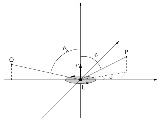
Figure 1: Boyer-Lindquist coordinates in a Kerr metric, also referred as spin-oriented coordinates in the text. $L$ is the black hole with spin $a$. $O$ is the observer and $P$ is a generic point. The gray disk visualizes the equatorial plane of the black hole.

Lightlike geodesics can be expressed in the following form in terms of the first integrals of motion $J$ and $Q$ found by Carter Car

$$\pm\int\frac{dx}{\sqrt{R}}=\pm\int\frac{d\vartheta}{\sqrt{\Theta}}$$ (5)

$$\phi_{f}-\phi_{i}= a\int\frac{x^{2}+a^{2}-aJ}{\Delta\sqrt{R}}dx-a\int\frac{dx}{\sqrt{R}}$$

$$+J\int\frac{\csc^{2}\vartheta}{\sqrt{\Theta}}d\vartheta,$$

where

$$\Theta= Q+a^{2}\cos^{2}\vartheta-J^{2}\cot^{2}\vartheta$$ (7)

$$R= x^{4}+(a^{2}-J^{2}-Q)x^{2}+(Q+(J-a)^{2})x$$

$$-a^{2}Q,$$

and $\phi_{i}$ is the initial value of the azimuthal coordinate of the photon.

The roots of $R$ represent inversion points in the radial motion. In gravitational lensing we consider photons coming from infinity, grazing the black hole and going back to infinity. For such trajectories there is only one inversion point $x_{0}$, representing the closest approach distance. The minimum allowed value of $x_{0}$ can be found solving the equations $R(x)=0$ and $R^{\prime}(x)=0$ simultaneously. However, in Kerr black hole, we do not have a unique minimum closest approach $x_{m}$, but rather a continuous family of values which depend on the approach trajectory followed by the photon. In particular, it is possible to establish a relation among the minimum closest approach $x_{m}$ and the corresponding values of the constants of motion $J$ and $Q$, that we shall indicate by $J_{m}$ and $Q_{m}$ (see e.g. Ref. Cha )

$$J_{m}=\frac{x_{m}^{2}(2x_{m}-3)+a^{2}(1+2x_{m})}{a(1-2x_{m})}$$ (8)

$$Q_{m}=\frac{x_{m}^{3}\left[2a^{2}-x_{m}(x_{m}-3/2)^{2}\right]}{a^{2}(x_{m}-1/2)^{2}}.$$ (9)

$x_{m}$ also represents the radius of the unstable circular photon orbit. This radius is fixed to $3/2$ when $a=0$ (Schwarzschild black hole). In the case of Kerr black holes, $x_{m}$ may vary between two limiting values $x_{m+}$, $x_{m-}$, depending on the incoming direction of the photon. The two limiting values can be analytically obtained solving the equation $Q_{m}=0$ (in fact, it is possible to show that gravitational lensing trajectories cannot be realized for $Q<0$ Cha ). To the third order in $a$, they read BDLSS

$$x_{m\pm}=\frac{3}{2}\mp\frac{2}{\sqrt{3}}a-\frac{4}{9}a^{2}\mp\frac{20}{27\sqrt{3}}a^{3}+O(a^{4}).$$ (10)

For example, photons whose orbit lies on the equatorial plane may turn either in the same sense of the black hole (prograde photons) or in the opposite sense (retrograde photons). Prograde photons are allowed to get closer to the black hole, with a minimum closest approach given by $x_{m+}$, while retrograde photons must stay farther than $x_{m-}$, in order to be deflected without falling into the black hole. Photons whose orbit does not lie on the equatorial plane are characterized by intermediate values of $x_{m}$, with $Q_{m}>0$. Thus $x_{m}$ can be used to parametrize the family of unstable photon orbits allowed in Kerr metric or, equivalently, the incoming direction of the photon. The corresponding values of the constants of motion are uniquely determined by Eqs. (8) and (9).

Although exact expressions for $x_{m+}$ and $x_{m-}$ are available, it is convenient to start with a perturbative expansion ab initio in order to be prepared to face more complicated quantities in the following BDLSS . Throughout our treatment, only for $x_{m}$ we need to push the expansion to the third order, in order to obtain some quantities to the second order in $a$.

III The shadow of a Kerr black hole

The constants of motion $J$ and $Q$ have an immediate link to the position in the sky where the observer detects the photon. In fact, we can define angular coordinates $(\theta_{1},\theta_{2})$ on the observer sky centered on the black hole position. We choose the orientation of these coordinates in such a way that the spin axis of the black hole is projected on the $\theta_{2}$-axis (see Fig.2).

Figure 2: The shadow of the black hole in the observer sky for $a=0.1$ and different values of the observer position $\vartheta_{o}$. The solid line is for $\vartheta_{o}=\pi/2$ (equatorial observer), the dashed line is for $\vartheta_{o}=\pi/4$ and the dotted line is for $\vartheta_{o}=0$ (polar observer).

As shown in Ref. Cha , photons detected by the observer at angular coordinates $(\theta_{1},\theta_{2})$ are characterized by constants of motion given by

$$J=-\theta_{1}D_{OL}\sqrt{1-\mu_{o}^{2}},$$ (11)

$$Q=\theta_{2}^{2}D_{OL}^{2}+\mu_{o}^{2}(\theta_{1}^{2}D_{OL}^{2}-a^{2}).$$ (12)

These relations can be easily recovered taking the limit for large distances in the equations of motion of the photon. They show that $J$ can be identified with the component of the orbital angular momentum of the photon along the spin axis, whereas $Q+J^{2}+\mu_{o}^{2}a^{2}$ is the squared total angular momentum of the photon.

Note that, with our choice of $(\theta_{1},\theta_{2})$, in the limit of equatorial observer $\mu_{o}=0$, prograde photons ($J>0$, $Q=0$) are detected by the observer on the left side of the black hole, while retrograde photons ($J<0$, $Q=0$) are detected on the right side. Conversely, in the limit of polar observers ($\mu_{o}\rightarrow\pm 1$), the projected angular momentum $J$ vanishes, while $Q\rightarrow(\theta_{1}^{2}+\theta_{2}^{2})D_{OL}^{2}-a^{2}$.

Inverting Eqs. (11) and (12), we find the position $(\theta_{1},\theta_{2})$ in the sky where the photon is detected with given constants of motion $J$ and $Q$, apart from an ambiguity in the sign of $\theta_{2}$

$$\theta_{1}=-\frac{J}{D_{OL}\sqrt{1-\mu_{o}^{2}}},$$ (13)

$$\theta_{2}=\pm D_{OL}^{-1}\sqrt{Q+\mu_{o}^{2}\left(a^{2}-\frac{J^{2}}{1-\mu_{o}^{2}}\right)}.$$ (14)

These relations can be used to convert the locus $(J_{m},Q_{m})$, parametrized by $x_{m}$ according to Eqs. (8) and (9) in the $(J,Q)$-space, into a new one $(\theta_{1,m},\theta_{2,m})$ in the observer sky. However, not all values of $x_{m}$ in the range $[x_{m+},x_{m-}]$ are acceptable. This can be easily understood, as photons lying on the equatorial plane can never reach non-equatorial observers. The reality condition for $\theta_{2,m}$ restricts $x_{m}$ to the range $[x_{p+},x_{p-}]$, where $x_{p+}$ and $x_{p-}$ are the roots of the equation $\theta_{2,m}=0$. To third order in $a$, these quantities read

$$x_{p\pm}= \frac{3}{2}\mp\frac{2}{\sqrt{3}}a\sqrt{1-\mu_{o}^{2}}-\frac{4}{9}a^{2}(1+\mu_{o}^{2})$$ (15)

$$\mp\frac{4}{27\sqrt{3}}a^{3}(5+6\mu_{o}^{2})\sqrt{1-\mu_{o}^{2}}+O(a^{4}).$$

Comparing with Eq. (10), we see that $x_{p\pm}\rightarrow x_{m\pm}$ in the limit $\mu_{o}\rightarrow 0$. On the other hand, when $\mu_{o}\rightarrow\pm 1$, the allowed range for $x_{m}$ shrinks to a single value $x_{p}\rightarrow\frac{3}{2}-\frac{8}{9}a^{2}$. This witnesses that when the observer is on the polar axis the axial symmetry of the lensing configuration is restored and all unstable photon orbits have the same radius again.

When $a$ vanishes, $x_{p+}$ and $x_{p-}$ both coincide with the Schwarzschild photon sphere radius, $3/2$, while, when $a$ is not zero, they are distinct and every value of $x_{m}$ in the interval $[x_{p+},x_{p-}]$ uniquely fixes the amplitude of the oscillation of the photon orbit on the equatorial plane, as we shall see later. On the basis of this consideration, in Paper I (with $\mu_{o}=0$) we introduced a parametrization of $x_{m}$ in the range $[x_{m+},x_{m-}]$, replacing $a$ with $a\xi$ in Eq. (10), with the parameter $\xi$ varying in the range $[-1,1]$.

In order to take into account the changes from Eq. (10) to (15), we have to update such parametrization, since it is not directly applicable to the case $\mu_{o}\neq 0$. Our new parametrization for $x_{m}$ is

$$x_{m}= \frac{3}{2}-\frac{2}{\sqrt{3}}a\xi\sqrt{1-\mu_{o}^{2}}-\frac{4}{9}a^{2}(1+\mu_{o}^{2})$$ (16)

$$-\frac{4}{27\sqrt{3}}a^{3}\xi(5+6\mu_{o}^{2})\sqrt{1-\mu_{o}^{2}}+O(a^{4}).$$

As $\xi$ varies in the interval $[-1,1]$ we get all possible values of $x_{m}$ in the interval $[x_{p+},x_{p-}]$. It will become clear later that $\xi$ is strictly related to the position angle of the generic point in the observer sky.

With this parametrization, we can rewrite Eqs.(8)-(9) to the second order in $a$ as

$$J_{m}(\xi)= \frac{3\sqrt{3}}{2}\xi\sqrt{1-\mu_{o}^{2}}-a(1-\mu_{o}^{2})(1+\xi^{2})$$ (17)

$$-a^{2}\frac{\xi\sqrt{1-\mu_{o}^{2}}}{3\sqrt{3}}[5-2\xi^{2}-2\mu_{o}^{2}(1-\xi^{2})],$$

$$Q_{m}(\xi)= \frac{27}{4}\left[1-(1-\mu_{o}^{2})\xi^{2}\right]$$ (18)

$$-3\sqrt{3}a\xi\sqrt{1-\mu_{o}^{2}}[1+\mu_{o}^{2}-(1-\mu_{o}^{2})\xi^{2}]$$

$$-a^{2}[(1+\mu_{o}^{2})^{2}-4(1-\mu_{o}^{2})\xi^{2}$$

$$+3(1-\mu_{o}^{2})^{2}\xi^{4}].$$

Notice that the presence of $a$ in the denominators of Eqs.(8)-(9) allows $\xi$ to be present already in the zero-order terms in Eqs.(17)-(18), permitting the use of the $\xi$-parametrization in Schwarzschild spacetime as well. However, since this parametrization has been introduced in a slightly different way w.r.t. Paper I, the expressions derived here cannot be directly compared to those of Paper I, except for those quantities that are independent of $\xi$. For example, eliminating $\xi$ from Eqs. (17) and (18), one can derive an expression for the locus $(J_{m},Q_{m})$ in the form $Q_{m}(J_{m})$. Doing the same with the expressions of Paper I, one would indeed find the same function $Q_{m}(J_{m})$ in the limit $\mu_{o}\rightarrow 0$.

Inserting Eqs. (17) and (18) in Eqs. (13)-(14) we get

$$D_{OL}\theta_{1,m} =-\frac{3\sqrt{3}}{2}\xi+a\sqrt{1-\mu_{o}^{2}}(1+\xi^{2})$$ (19)

$$+a^{2}\frac{\xi}{3\sqrt{3}}[5-2\mu_{o}^{2}-2\xi^{2}(1-\mu_{o}^{2})],$$

$$D_{OL}\theta_{2,m} =\pm\frac{3\sqrt{3}}{2}\sqrt{1-\xi^{2}}\mp a\xi\sqrt{1-\xi^{2}}\sqrt{1-\mu_{o}^{2}}$$ (20)

$$\mp a^{2}\frac{\sqrt{1-\xi^{2}}}{3\sqrt{3}}[1+2\mu_{o}^{2}-2\xi^{2}(1-\mu_{o}^{2})].$$

This locus is formed by the points in the observer sky where photons with minimum closest approach would show up. No gravitational lensing images are possible inside this locus, which is thus also known as the shadow of the black hole. In Fig. 2 we show it for different values of $\mu_{o}$. Note that, to zero order, $\theta_{1,m}\propto-\xi$ and $\theta_{2,m}\propto\sqrt{1-\xi^{2}}$, justifying the identification of $\xi$ with the cosine of the position angle in the $(\theta_{1},\theta_{2})$ plane as taken from the opposite of the $\theta_{1}$-axis. This fact facilitates the physical interpretation of the parameter $\xi$.

The shadow of the black hole is the first observable in extreme gravitational lensing by supermassive black holes. It thus deserves some further analysis in order to understand the effect of the spin and the observer position.

First we note that $\theta_{1,m}$ and $\theta_{2,m}$, to second order in $a$, satisfy the ellipse equation

$$\frac{(\theta_{1,m}-\theta_{0})^{2}}{A_{1}^{2}}+\frac{\theta_{2,m}^{2}}{A_{2}^{2}}=1$$ (21)

with the origin shifted rightward by

$$\theta_{0}=\frac{2a\sqrt{1-\mu_{o}^{2}}}{D_{OL}},$$ (22)

and semiaxes given by

$$A_{1}=D_{OL}^{-1}\left(\frac{3\sqrt{3}}{2}-\frac{a^{2}}{\sqrt{3}}\right)$$ (23)

$$A_{2}=D_{OL}^{-1}\left(\frac{3\sqrt{3}}{2}-\frac{a^{2}}{\sqrt{3}}\mu_{o}^{2}\right).$$ (24)

By these analytical expressions for the shadow, we can make several considerations. The presence of a non-vanishing spin causes a slight distortion and a displacement of the shadow from the black hole position. When the observer lies on the spin axis ($\mu_{o}=\pm 1$), the axial symmetry is restored and the shadow returns to be centered on the black hole and circular. However, even in this limiting case, the radius of the shadow is no longer $3\sqrt{3}/2$ as in Schwarzschild, but it is slightly smaller, being $3\sqrt{3}/2-a^{2}/\sqrt{3}$.

It has been proposed that the observation of the shape of the shadow of a black hole by VLBI may help to determine the parameters of a Kerr black hole, such as its mass, its angular momentum and the inclination of the spin FMA ; Zak . However, both in the shift $\theta_{0}$ and in the ellipticity

$$e\equiv\frac{A_{2}-A_{1}}{A_{2}}=\frac{2}{9}a^{2}(1-\mu_{o}^{2})$$ (25)

the black hole spin and the observer declination appear in the same combination $a\sqrt{1-\mu_{o}^{2}}=a\sin\vartheta_{o}$, which represents the projection of the spin on a plane orthogonal to the line of sight. Thus it is impossible to determine both the absolute value of the spin and its inclination from the shape of the shadow. The only possibility is that we already know the distance $D_{OL}$ and the mass of the black hole to such accuracy that we are able to extract $a$ from a measure of the minor semi-axis $A_{1}$ solely. However, since the spin contribution to the major semi-axis is only of second order in $a$, we need a very high accuracy in the shadow observation in order to appreciate such a small contribution. For example, if $a=0.1$, the spin contribution to $A_{1}$ is of order $0.2\%$. As already pointed in Ref. Zak by numerical examples, the disentanglement of $a$ and $\vartheta_{o}$ is only possible for values of the black hole spin very close to the extremal case. By our perturbative formulae, we have justified this claim analytically. Of course, for high values of $a$, when higher orders contribute to determine the shape of the shadow, the degeneracy between $a$ and $\vartheta_{o}$ can be broken, in agreement with what stated in Ref. Zak .

It has been pointed out in Paper I that as long as we deal with Kerr black holes with spin smaller than $a=0.2$, the perturbative approximation works surprisingly well. Then, the degeneracy between $a$ and $\vartheta_{o}$ in the shadow of the black hole poses a serious difficulty to the determination of the parameters of the black hole by the simple observation of the shadow. As we shall see in the next sections, this degeneracy plagues all gravitational lensing observables in different degrees.

IV Kerr lensing in the Strong Deflection Limit

As in Paper I, we introduce the following parametrization of the observer sky

$$\left\{\begin{array}[]{l}\theta_{1}(\epsilon,\xi)=\theta_{1,m}(\xi)(1+\epsilon)\\ \theta_{2}(\epsilon,\xi)=\theta_{2,m}(\xi)(1+\epsilon)\end{array}\right..$$ (26)

Varying $\xi$ in the range $[-1,1]$ and $\epsilon$ in the range $[-1,\infty]$, we can obviously cover the whole upper half of the observer sky, since $\xi$ establishes the position angle of the light ray w.r.t. the $(-\theta_{1})-$axis (through Eqs. (19) and (20)) whereas $\epsilon$ fixes the angular distance from the shadow of the black hole. In fact, in the following, $\epsilon$ will be generically referred to as the separation from the shadow of the black hole.

We are interested into light rays experiencing very large deflections by a Kerr black hole. These light rays reach the observer from directions $(\theta_{1},\theta_{2})$ very close to the shadow. In the parametrization (26), they are thus characterized by a very small positive $\epsilon$, while keeping $\xi$ in the whole range $[-1,1]$. The SDL amounts to performing the integrals in the geodesics equations (5)-(5), to the lowest orders in the separation from the shadow $\epsilon$.

The values of the constants of motion $J$ and $Q$, corresponding to such strongly deflected photons, can be found using Eqs. (11)-(12):

$$J(\xi,\epsilon)= J_{m}(\xi)(1+\epsilon)$$ (27)

$$Q(\xi,\epsilon)= Q_{m}(\xi)(1+2\epsilon)+2a^{2}\epsilon\mu_{o}^{2}.$$ (28)

Substituting these expressions in Eq. (7) and solving the equation $R=0$ for $x_{0}$, we get the closest approach distance as

$$\!\!\!\!\!\!\!\!\!\!\!\!\!\!\!x_{0}(\xi,\delta)=x_{m}(\xi)(1+\delta)$$ (29)

$$\!\!\!\!\!\!\!\!\!\!\!\!\!\!\!\delta=\sqrt{\frac{2\epsilon}{3}}\left[1-\frac{2}{3\sqrt{3}}a\hat{\xi}+\frac{2}{27}a^{2}(10-\mu_{o}^{2}-14\hat{\xi}^{2})\right]$$ (30)

where we have introduced the compact notation

$$\hat{\xi}=\xi\sqrt{1-\mu_{o}^{2}}.$$ (31)

As $\epsilon$ represents the separation of the image in the observer sky from the shadow of the black hole, $\delta$ represents the relative difference between the closest approach $x_{0}$ and the minimum closest approach $x_{m}(\xi)$ fixed by the position angle through $\xi$. It will be synthetically called approach parameter. As $\delta$ decreases, we expect the deflection to increase more and more. In the limit $\delta\rightarrow 0$, the photon is injected into the unstable orbit with radius $x_{m}(\xi)$. Conversely, photons with a large approach parameter are weakly deflected. Of course, the relation between $\epsilon$ and $\delta$ ensures that the SDL can be equivalently stated in terms of either of the two parameters.

Let us introduce our gravitational lensing configuration. As said before, the observer is at radial coordinate $D_{OL}$, at polar angle $\vartheta_{o}$ and azimuthal angle $\phi_{o}=\pi$. We will call optical axis the line connecting the lens and the observer. The source is assumed to be static at Boyer-Lindquist coordinates $(D_{LS},\vartheta_{s},\phi_{s})$.

Our lens equations are provided by Eqs. (5)-(5), where we identify the final value of the azimuthal coordinate with the observer’s one ($\phi_{f}=\phi_{o}=\pi$), and the initial value with the source’s one $\phi_{i}=\phi_{s}$. In these equations there are two radial integrals and two angular integrals. The radial integrals are solved using the SDL technique and expanding all coefficients to second order in $a$, as in Paper I. The results of this procedure are reported in Appendix A. Similarly, the angular integrals are solved to second order in $a$ in Appendix B.

Once all integrals are calculated, we have to solve Eqs. (5)-(5) in terms of the source coordinates $(\phi_{s},\mu_{s})$, so that they are in the lens map form

$$\left\{\begin{array}[]{l}\mu_{s}=\mu_{s}(\delta,\xi)\\ \phi_{s}=\phi_{s}(\delta,\xi)\end{array}\right..$$ (32)

Note that the lens equation will be written in terms of the approach parameter $\delta$ and the position angle through $\xi$. Through Eqs. (30) and (26) we can then go back to the coordinates in the observer sky $(\theta_{1},\theta_{2})$.

In the following sections, we will calculate the critical curves and the caustics of the Kerr gravitational lens order by order. The procedure is indeed identical to that described in Paper I, save for the complication introduced by the additional parameter $\mu_{o}$. However, once we manage to recast all equations in the best forms, the results remain very simple, so that a thorough discussion of the effects of spin and observer colatitude is possible.

V Derivation of the relativistic caustics

V.1 Zero-order caustics

The first task is to recover the results for a Schwarzschild black hole, imposing the limit $a\rightarrow 0$.

Using the results of Appendices A and B to the zero-order, Eqs. (5) and (5) read respectively

$$\psi =m\pi\mp\arcsin\frac{\mu_{s}}{\sqrt{1-{\hat{\xi}}^{2}}}$$ (34)

$$\pm(-1)^{m}\arcsin\frac{\mu_{o}}{\sqrt{1-{\hat{\xi}}^{2}}},$$

$$\phi_{s} =\pi-Sign[\xi]m\pi\pm\arctan\frac{\mu_{s}{\hat{\xi}}}{\sqrt{1-\mu_{s}^{2}-{\hat{\xi}}^{2}}}$$

$$\mp(-1)^{m}\arctan\frac{\mu_{o}{\hat{\xi}}}{\sqrt{1-\mu_{o}^{2}-{\hat{\xi}}^{2}}},$$

where the new variable

$$\psi=-2\log\delta+2\log[12(2-\sqrt{3})],$$ (35)

allows us to put the equations in a very compact form. $\psi$ actually coincides with the deflection induced by a Schwarzschild black hole with the same mass of our Kerr black hole. On the ground of this connection, we shall often refer to $\psi$ as “scalar deflection” in the following.

The double signs coming from the angular integrals must be treated as follows: if the photon moves out of the source increasing its initial value of $\mu$, then we must choose the upper signs, otherwise we will select the lower signs. These double signs are the relics of those present in Eqs. (5) and (5). For more details about their origin, the reader is referred to the Appendix B. $m$ represents the number of inversions in the polar motion of the photon.

Introducing the quantity

$$\psi_{o}=\mp(-1)^{m}\arcsin\frac{\mu_{o}}{\sqrt{1-{\hat{\xi}}^{2}}},$$ (36)

we can easily solve Eqs. (34)-(34) w.r.t. $\phi_{s}$ and $\mu_{s}$ to get the zero-order lens equation

$$\mu_{s} =\mp(-1)^{m}\sqrt{1-{\hat{\xi}}^{2}}\sin(\psi+\psi_{o}),$$ (38)

$$\phi_{s} =\pi(1-m)+\arctan\left[\hat{\xi}\tan\psi_{o}\right]$$

$$-\arctan\left[\hat{\xi}\tan(\psi+\psi_{o})\right].$$

Since the azimuth $\phi$ is a coordinate with period $2\pi$, we have eliminated the $Sign[\xi]$ in front of $m\pi$ in Eq. (38). In the derivation of Eq. (38) from Eqs. (34) and (38), we have used the relations

$$\frac{\mu_{s}}{\sqrt{1-\mu_{s}^{2}-{\hat{\xi}}^{2}}}=\mp\tan(\psi+\psi_{o})$$ (39)

$$\frac{\mu_{o}}{\sqrt{1-\mu_{o}^{2}-{\hat{\xi}}^{2}}}=\mp(-1)^{m}\tan\psi_{o}$$ (40)

and exploited the fact that the number of inversions in the polar motion is just the integer part of $(\psi+\psi_{o}+\pi/2)/\pi$.

Let us understand the meaning of the zero-order lens equations. Eq. (38) states that the photon performs symmetric oscillations on the equatorial plane (recall that $\mu\equiv\cos\vartheta$) with amplitude $\sqrt{1-\hat{\xi}^{2}}$, which depends on the observer declination and the trajectory chosen by the photon (polar $\hat{\xi}=0$, equatorial $\hat{\xi}=\pm 1$ or whatever). The number of oscillations depends on the scalar deflection $\psi$, which diverges when the approach parameter $\delta\rightarrow 0$. $\psi_{o}$ is the initial condition of the oscillation, which depends on the observer declination. The double signs take into account the fact that the oscillations occur in opposite ways depending on the starting sign of $\dot{\mu}$.

Eq. (38) is the azimuthal motion of the photon. It can be better understood when we choose equatorial photons with $\hat{\xi}=1$. Then it just reduces to $\phi=\pi-\psi$, which states that the azimuthal shift is the scalar deflection minus $\pi$, as expected in this simple case. Different values of $\xi$ need to be analyzed by some spherical trigonometry, in order to understand the trigonometric functions in Eq. (38).

After the zero order lens equation is constructed, we can study the structure of critical curves and caustics. The Jacobian of the lens map, $D$, can be easily calculated from (38) and (38). We find

$$\frac{\partial\mu_{s}}{\partial\xi}=\pm(-1)^{m}\frac{\hat{\xi}\sqrt{1-{\mu_{o}}^{2}}}{\sqrt{1-{\hat{\xi}}^{2}}}\sec\psi_{o}\sin\psi$$ (41)

$$\frac{\partial\mu_{s}}{\partial\psi}=\mp(-1)^{m}\sqrt{1-{\hat{\xi}}^{2}}\cos(\psi+\psi_{o})$$ (42)

$$\frac{\partial\phi_{s}}{\partial\xi}=-\frac{\cos(\psi+\psi_{o})\sec\psi_{o}\sin\psi}{\sqrt{1-\mu_{o}^{2}}}$$ (43)

$$\frac{\partial\phi_{s}}{\partial\psi}=-\frac{\hat{\xi}\sec^{2}(\psi+\psi_{o})}{1+{\hat{\xi}}^{2}\tan^{2}(\psi+\psi_{o})}$$ (44)

and using Eqs. (31) and (36), we finally have

$$D=\frac{\partial\mu_{s}}{\partial\xi}\frac{\partial\phi_{s}}{\partial\psi}-\frac{\partial\mu_{s}}{\partial\psi}\frac{\partial\phi_{s}}{\partial\xi}=\mp(-1)^{m}\frac{\sin\psi}{\sqrt{1-{\xi}^{2}}}.$$ (45)

Since all transformations from $(\psi,\xi)$ to $(\theta_{1},\theta_{2})$ are non-singular (except for the points $\xi=\pm 1$), the solutions of the equation $D=0$ determine the critical curves. To zero order we have

$$\psi_{k}=k\pi.$$ (46)

As expected, the critical curves correspond to values of the scalar deflection that are multiples of $\pi$. Having introduced the most generic coordinate system for the black hole has not prevented us from recovering the Schwarzschild result. Through Eqs. (35), (30) and (26) we reconstruct the critical curves in the observer coordinates

$$\begin{array}[]{l}D_{OL}\theta_{1,k}(\xi)=-\frac{3\sqrt{3}\xi}{2}\left[1+\epsilon_{k}\right]\\ \\ D_{OL}\theta_{2,k}(\xi)=\pm\frac{3\sqrt{3}}{2}\sqrt{1-\xi^{2}}\left[1+\epsilon_{k}\right]\end{array},$$ (47)

where

$$\epsilon_{k}=216(2-\sqrt{3})^{2}e^{-k\pi}$$ (48)

is the separation of the critical curve from the shadow.

We will refer to the integer number $k$ as the critical curve (or caustic) order. Eqs. (47) describe a series of concentric rings, parametrized by $\xi$, slightly larger than the shadow of the black hole and whose radius $\frac{3\sqrt{3}}{2}(1+\epsilon_{k})$ exponentially decreases to the shadow radius with increasing critical curve order.

The equations of the caustics are easily found introducing Eq. (46) into (38)-(38) and exploiting the fact that the number of inversions $m$ coincides with $k$ if $\psi=k\pi$. We have

$$\mu_{s}=(-1)^{k}\mu_{o},~{}~{}\phi_{s}=(1-k)\pi.$$ (49)

As already known, the Schwarzschild caustics are point-like and lie on the optical axis. They are in front of the black hole ($\mu_{s}=\mu_{o}$, with $\phi_{s}$ being an odd multiple of $\pi$) for even values of $k$ (retrolensing caustics), and behind it ($\mu_{s}=-\mu_{o}$, with $\phi_{s}$ being an even multiple of $\pi$) for odd $k$ (standard lensing).

The SDL description is limited to large deflections ($\psi\gtrsim\pi$), thus working better and better for higher order caustics Boz1 ; S1-S14 . It cannot be applied to the first order one ($k=1$) whose full description can be derived in the weak deflection limit for sources sufficiently far from the lens. In what follows, we focus on caustics of order $k\geq 2$ and investigate how their structure is affected by the concomitant action of the lens spin and the observer declination.

V.2 First-order caustics

We now introduce first order corrections to the zero-order solutions found in the previous section. Starting from the results of Appendix A and B, we solve the lens equations perturbatively adding the first order terms to Eqs. (38)-(38), obtaining

$$\mu_{s}= \mp(-1)^{m}\sqrt{1-{\hat{\xi}}^{2}}\sin(\psi+\psi_{o})$$ (50)

$$\mp(-1)^{m}\frac{2a\hat{\xi}}{3\sqrt{3}}\sqrt{1-{\hat{\xi}}^{2}}\cos\psi_{o}\sin\psi,$$

$$\phi_{s}= (1-m)\pi+\arctan\left[\hat{\xi}\tan\psi_{o}\right]$$ (51)

$$-\arctan\left[\hat{\xi}\tan(\psi+\psi_{o})\right]$$

$$-\frac{4a}{3\sqrt{3}}\left[\psi+3\sqrt{3}\log(2\sqrt{3}-3)\right.$$

$$\left.-\frac{1-{\hat{\xi}}^{2}}{2}\frac{\cos(\psi+\psi_{o})\sin\psi\cos\psi_{o}}{1-(1-{\hat{\xi}}^{2})\sin^{2}(\psi+\psi_{o})}\right].$$

The Jacobian of the lens equation to first order is

$$D=\mp(-1)^{m}\frac{\sin\psi}{\sqrt{1-{\xi}^{2}}}\left(1+\frac{2a\xi\sqrt{1-\mu_{o}^{2}}}{\sqrt{3}}\right),$$ (52)

which is always solved by Eq. (46), thus implying that the scalar deflection $\psi$ and consequently the approach parameter $\delta$ are not affected by lens spinning to the first order. Anyway, due to the spin dependence in Eq. (30), first order corrections modify the separation of the critical curves from the shadow. They read

$$D_{OL}\theta_{1,k}= -\frac{3\sqrt{3}\xi}{2}(1+\epsilon_{k})+$$ (53)

$$a\left[1+\xi^{2}+\epsilon_{k}(1-\xi^{2})\right]\sqrt{1-{\mu_{o}}^{2}},$$

$$D_{OL}\theta_{2,k}= \pm\frac{3\sqrt{3}(1+\epsilon_{k})\sqrt{1-\xi^{2}}}{2}\mp$$

$$a\xi\sqrt{1-\xi^{2}}(1-\epsilon_{k})\sqrt{1-{\mu_{o}}^{2}},$$

where $\epsilon_{k}$ is still the zero-order separation defined in Eq. (48).

Coming to the caustics, from Eqs. (50)-(51) and (46) we get

$$\mu_{s}=(-1)^{k}\mu_{o},$$ (54)

$$\phi_{s}=\pi(1-k)-\Delta\phi_{k}$$ (55)

$$\Delta\phi_{k}=4a\left[\frac{k\pi}{3\sqrt{3}}-\log(2\sqrt{3}-3)\right].$$ (56)

So, caustics are still point-like but the alignment with the optical axis is now missing because of first order corrections, as already pointed out in Paper I. The azimuthal shift is proportional to the caustic order, it does not depend on the observer declination and is negative, thus implying a clockwise drift, if we look at the black hole from the north pole. This means that, as $k$ is still the number of inversion points, prograde (retrograde) light rays, emitted by a source on a caustic point, perform more (respectively less) than $(k-1)/2$ loops. Moreover, as the caustics drift from the optical axis and from each other, perfect alignment of observer, lens and source is not required for the enhancement of the images which are enhanced one at a time, as sources cannot cross more than one caustic point at the same time. For numerical values of the shift see Paper I, Table 1.

V.3 Second-Order Caustics

In this section we investigate the effects of second order corrections in the black hole spin on the critical curves and caustics. Following the same steps as in the previous subsection, we can add the second order terms $a^{2}\delta\mu_{s}^{(2)}$ to Eqs. (50) and $a^{2}\delta\phi_{s}^{(2)}$ to (51). Since they have quite long expressions, we report them in Appendix C and proceed with the analysis of the second order lens equation. In fact, although the general second order lens equation is quite involved, it is easy to solve the Jacobian determinant equation $D=0$ in terms of the second order perturbation of $\psi$, starting from the zero order solution (46). We get

$$\psi_{k}=k\pi+a^{2}\delta\psi,$$ (57)

where

$$\delta\psi= -\frac{1}{18}\left[9c_{k}(3-2\mu_{o}^{2}-3\hat{\xi}^{2})+32(1-\hat{\xi}^{2})\right]$$ (58)

and

$$c_{k}=\frac{2}{9}(5k\pi+8\sqrt{3}-36).$$ (59)

Using Eqs. (35) and (30) we can calculate the second order corrections to the approach parameter $\delta$ and the separation from the shadow $\epsilon$. After that, by Eqs. (26), we can derive the second order corrections to the critical curves given in Eq. (53)

$$\begin{array}[]{lll}D_{OL}\theta_{1,k}^{(2)}&=&a^{2}\frac{\xi}{3\sqrt{3}}\left[5-2\mu_{o}^{2}-2\hat{\xi}^{2}\right.\\ &&\left.+\epsilon_{k}\left(29-8\mu_{o}^{2}-32\hat{\xi}^{2}\right)\right],\\ \\ D_{OL}\theta_{2,k}^{(2)}&=&\mp a^{2}\frac{\sqrt{1-\xi^{2}}}{3\sqrt{3}}\left[1+2\mu_{o}^{2}-2\hat{\xi}^{2}\right.\\ &&\left.+\epsilon_{k}\left(21-32\hat{\xi}^{2}\right)\right],\end{array}$$ (60)

where the zero-order separation $\epsilon_{k}$ is always given by Eq. (48).

Plugging Eq. (57) into the lens map, we get the caustics parametric equations up to the second order in $a$:

$$\mu_{s}=(-1)^{k}\mu_{o}\pm a^{2}c_{k}(1-{\mu_{o}}^{2})^{3/2}(1-\xi^{2})^{3/2},$$ (61)

$$\phi_{s}=(1-k)\pi-\Delta\phi_{k}-a^{2}c_{k}\xi^{3}\sqrt{1-{\mu_{o}}^{2}}.$$ (62)

As explained in Section V.1, the double sign in Eq. (61) allows for the possibilities that the photon starts its journey by increasing $\mu$ or by decreasing $\mu$, respectively. it is necessary to take both possibilities into account in order to cover the whole caustic. In agreement with Paper I and other works where the same results are found numerically (e.g.RauBla ), we get extended caustics whose shape is a 4-cusped astroid, with cusps in $\xi=\pm 1$ and $\xi=0$ (for different signs of initial $\dot{\mu}$). The extension of the caustics along $\mu$ and along $\phi$ is different. However, choosing appropriate coordinates centered on the caustic, it is possible to show that the extension in the sky as seen by the black hole is the same along both axes (see next subsection).

V.4 Observables related to critical curves and caustics

After second order corrections to critical curves and caustics have been derived, we can discuss their dependence on $a$ and $\vartheta_{o}$.

First we note that the critical curves obtained adding Eq. (60) to (53) satisfy the ellipse equation

$$\frac{(\theta_{1,k}-\theta_{0})^{2}}{A_{1,k}^{2}}+\frac{\theta_{2,k}^{2}}{A_{1,k}^{2}}=1$$ (63)

with the same origin shift as the shadow (Eq. (22)) and semiaxes given by

$$A_{1,k} =D_{OL}^{-1}\left\{\frac{3\sqrt{3}}{2}(1+\epsilon_{k})\right.$$ (65)

$$\left.-a^{2}\frac{4-\epsilon_{k}(4-9c_{k}\mu_{o}^{2})}{4\sqrt{3}}\right\}$$

$$A_{2,k} =D_{OL}^{-1}\left\{\frac{3\sqrt{3}}{2}-\left[16\epsilon_{k}^{2}-4(3+\epsilon_{k}^{2})\mu_{o}^{2}\right.\right.$$

$$\left.\left.\!\!\!\!\!\!\!\!\!\!\!+27c_{k}\epsilon_{k}(1+\epsilon_{k})(3-2\mu_{o}^{2})\right]\frac{a^{2}}{12\sqrt{3}(1+\epsilon_{k})}\right\}.$$

The critical curves tend to coincide with the shadow in the limit $k\rightarrow\infty$, which corresponds to photons winding an infinite number of times, thus tending to the unstable photon orbit. The ellipticity of the critical curves is

$$e=a^{2}(1-\mu_{o}^{2})\frac{4(3+\epsilon_{k}^{2})+81c_{k}\epsilon_{k}(1+\epsilon_{k})}{54(1+\epsilon_{k})^{2}},$$ (66)

which is slightly higher than that of the shadow for the lower order critical curves, but tends to that of the shadow as $k\rightarrow\infty$. In particular, we see that shift and ellipticity of the critical curves still depend on the combination $a\sin\vartheta_{o}$, as for the shadow. So, even the observation of several critical curves cannot help to determine $a$ and $\vartheta_{o}$ separately.

Let us come to the caustics. Here the situation is more subtle and needs to be investigated with grain of salt.

Suppose we have no independent knowledge of the direction of the black hole spin or, at least, the direction of the spin is not known to any great accuracy. Then, the observer will construct his coordinates allowing for a non-vanishing position angle $\nu$ for the spin axis. The uncertainty in $\nu$ will be determinant in the following discussion. Let us thus introduce $(x,\hat{\vartheta},\hat{\phi})$ as observer-oriented coordinates, still centered at the black hole, but with the polar axis perpendicular to the optical axis and the azimuth $\hat{\phi}$ taken from the direction opposite to the observer. In general, if the observer ignores the spin axis, the spin axis of the black hole would have a position angle $\nu$ from the polar axis as fixed by the observer. The coordinate transformation from $(\mu,\phi)$ to $(\hat{\vartheta},\hat{\phi})$ is

$$\hat{\vartheta} =\arccos\left[\mu\sqrt{1-\mu_{o}^{2}}\cos\nu+\mu_{o}\sqrt{1-\mu^{2}}\cos\phi\cos\nu\right.$$ (68)

$$\left.+\sqrt{1-\mu^{2}}\sin\phi\sin\nu\right]$$

$$\hat{\phi} =\arctan\left[\left(\sqrt{1-\mu^{2}}\sin\phi\cos\nu\right.\right.$$

$$\left.-\mu_{o}\sqrt{1-\mu^{2}}\cos\phi\sin\nu-\mu\sqrt{1-\mu_{o}^{2}}\sin\nu\right)$$

$$\left.\cdot\left(\sqrt{1-\mu^{2}}\sqrt{1-\mu_{o}^{2}}\cos\phi-\mu\mu_{o}\right)^{-1}\right].$$

Fig. 3 illustrates the geometrical meaning of these coordinates.

Figure 3: Observer-oriented coordinates $(\hat{\vartheta},\hat{\phi})$ introduced in the text. $L$ is the black hole with spin $a$. $O$ is the observer and $P$ is a generic point. $\vartheta_{o}$ is the inclination of the spin on the line of sight, $\nu$ is the position angle of the spin.

Transforming the caustics (61)-(62) from the spin-oriented coordinates $(\mu,\phi)$ to the observer-oriented coordinates $(\hat{\vartheta},\hat{\phi})$, and expanding to second order in $a$, we get

$$\hat{\vartheta}_{s} =\frac{\pi}{2}-(-1)^{k}\Delta\phi_{k}\sqrt{1-\mu_{o}^{2}}\sin\nu$$ (70)

$$-(-1)^{k}\frac{1}{2}\Delta\phi_{k}^{2}\mu_{o}\sqrt{1-\mu_{o}^{2}}\cos\nu$$

$$\!\!\!\!\!\!\!\!\!\!-R_{k}\left[(-1)^{k}\xi^{3}\sin\nu\pm(1-\xi)^{3/2}\cos\nu\right]$$

$$\hat{\phi}_{s} =(1-k)\pi-\Delta\phi_{k}\sqrt{1-\mu_{o}^{2}}\cos\nu$$

$$+\frac{1}{2}\Delta\phi_{k}^{2}\mu_{o}\sqrt{1-\mu_{o}^{2}}\sin\nu$$

$$\!\!\!\!\!\!\!\!\!\!-R_{k}\left[\xi^{3}\cos\nu\pm(-1)^{k}(1-\xi)^{3/2}\sin\nu\right],$$

where

$$R_{k}\equiv a^{2}c_{k}(1-\mu_{o}^{2})=\frac{2}{9}a^{2}(1-\mu_{o}^{2})(5k\pi+8\sqrt{3}-36)$$ (71)

is the semi-amplitude of the caustic. In fact, we can appreciate that, in observer-oriented coordinates, the extension of the caustic is the same in both polar and azimuthal directions, as anticipated before for any coordinate system centered on the caustic. So, the extension is quadratic in the spin and is maximal for equatorial observers, while the astroid shrinks to a single point when the observer lies on the spin axis. The caustic extension also increases linearly with the caustic order $k$.

Then, we note that the angular shift of the center of the caustic from the optical axis is

$$\Delta_{k} \equiv\arccos[\sin\hat{\vartheta}\cos\hat{\phi}]=\Delta\phi_{k}\sqrt{1-\mu_{o}^{2}}$$ (72)

$$=4a\sqrt{1-\mu_{o}^{2}}\left[\frac{k\pi}{3\sqrt{3}}-\log(2\sqrt{3}-3)\right].$$

It is linear in the black hole spin and the caustic order. Similarly to the semi-amplitude, also the shift is maximal for equatorial observers and vanishes for polar observers, when the axial symmetry is restored.

The shift and the semi-amplitude of the caustics are very easy quantities to determine in case of observation of the relativistic images generated by a source crossing a relativistic caustic. In fact, if the observer is able to identify the source and follow its direct image throughout the duration of the caustic crossing event, then he would immediately determine the position of the caustic and estimate its extension. Unfortunately, even in these two quantities, the black hole spin and the observer declination always appear in the combination $a\sqrt{1-\mu_{o}^{2}}=a\sin\vartheta_{o}$, making the breaking of the degeneracy between these two parameters impossible. On the other hand, it is easy to determine the order $k$ of the caustic involved in the lensing event, since the ratio

$$\frac{\Delta_{k}^{2}}{R_{k}}=\frac{8\left[k\pi+3\sqrt{3}\log(2\sqrt{3}-3)\right]^{2}}{3\left(5k\pi+8\sqrt{3}-36\right)}$$ (73)

only depends on $k$ and increases monotonically in $k$, without degeneracy between any two values.

One possibility for the separate determination of $a$ and $\mu_{o}$ arises in case the spin position angle $\nu$ is known to a very good accuracy from independent measures. Then we can move to a more convenient coordinate frame where $\nu=0$. If this is possible, looking at Eqs. (70) and (70) we see that the shift in the azimuthal direction is linear in $a$, while a residual quadratic shift is present in the polar direction, which amounts to

$$\delta_{k} \equiv\frac{1}{2}\Delta\phi_{k}^{2}\mu_{o}\sqrt{1-\mu_{o}^{2}}$$ (74)

$$=8a^{2}\mu_{o}\sqrt{1-\mu_{o}^{2}}\left[\frac{k\pi}{3\sqrt{3}}-\log(2\sqrt{3}-3)\right]^{2}.$$

Then, if one is able to measure this residual shift, one can extract the observer colatitude $\vartheta_{o}$ as

$$\cot\vartheta_{o}=\frac{2\delta_{k}}{\Delta_{k}^{2}}.$$ (75)

Once the observer position relative to the spin axis is known, we can use either $\Delta_{k}$ or $R_{k}$ to extract the black hole spin $a$. However, as for the case of the direct determination of $a$ from the measure of the minor semi-axis of the shadow, this is a higher order measure, which requires very accurate independent information.

Fig. 4 shows a caustic and illustrates the meaning of the semi-amplitude $R_{k}$, the horizontal shift $\Delta_{k}$ and the vertical shift $\delta_{k}$. The picture is done for a standard lensing caustic ($k$ odd) with $\vartheta_{o}>\pi/2$, so that the caustic is displaced upward (see Eq. (70)).

Figure 4: A typical caustic in Kerr lensing. The extension is the same in both directions. Having chosen coordinates such that the position angle of the spin vanishes, the caustic has an azimuthal shift $\Delta_{k}$ and a vertical shift $\delta_{k}$ w.r.t. the line of sight.

As usual we can trust our results as long as the perturbative terms remain small. In extremal or close-to-extremal Kerr black holes, higher orders in $a$ would play a major role in the critical curves and caustics profile. In that case, the degeneracy between $a$ and $\vartheta_{o}$ can be probably broken also through the determination of the extension and position of the caustics or through the analysis of the critical curves. However, in the literature there is no investigation of Kerr black holes with high spin that is deep enough to allow a comparison with our perturbative results for low spins.

VI Gravitational lensing near caustics

VI.1 Position of the relativistic images

Although in our picture the images cannot be found analytically for arbitrary source positions using the lens mapping that we have derived, they can be actually found for sources in the neighbourhood of a caustic. This is indeed the most interesting case, as the relativistic images are highly magnified and become observable only if this event occurs. Assuming that the angular distance between the source and a caustic of order $k$ is of the order of $a^{2}$ (thus comparable with the caustic semiaxis), we can write the source position as

$$\mu_{s}=(-1)^{k}\mu_{o}+a^{2}\delta\mu_{s},$$ (76)

$$\phi=(1-k)\pi-\Delta\phi_{k}+a^{2}\delta\phi_{s},$$ (77)

In this assumption, the images will be very close to the critical curve of order $k$. Then the scalar deflection will be

$$\psi=k\pi+a^{2}\delta\psi.$$ (78)

Plugging the last equation into the lens map written up to corrections of second order in $a$ and inverting with respect to $\delta\mu_{s}$ and $\delta\phi_{s}$, we get

$$\delta\mu_{s}= \mp\frac{1}{9}\sqrt{1-\mu_{o}^{2}}\sqrt{1-\xi^{2}}\left[9\delta\psi\right.$$ (79)

$$\left.+(5k\pi+8\sqrt{3}-20)(1-(1-{\mu_{o}}^{2})\xi^{2})\right],$$

$$\delta\phi_{s}= \frac{\xi}{9\sqrt{1-{\mu_{o}}^{2}}}\left[92-24\sqrt{3}-15k\pi-9\delta\psi\right.$$ (80)

$$+2{\mu_{o}}^{2}(5k\pi+8\sqrt{3}-36)$$

$$\left.+(5k\pi+8\sqrt{3}-20)(1-{\mu_{o}}^{2})\xi^{2}\right].$$

Solving (80) with respect to $\delta\psi$ and plugging its expression into (79), we find

$$\delta\mu_{s}\xi=-S(-1)^{k}(1-{\mu_{o}}^{2})(\delta\phi_{s}+c_{k}\sqrt{1-{\mu_{o}}^{2}}\xi)\sqrt{1-\xi^{2}},$$ (81)

where $c_{k}$ is given by Eq. (59) and $S=\mp(-1)^{k}$. This equation can be more conveniently written in terms of observer-oriented coordinates $(\hat{\vartheta}_{s},\hat{\phi}_{s})$. Supposing that the position angle of the spin has been well established by observations of the shadow or by the shift of the caustic itself, we put $\nu=0$ for simplicity and write

$$\hat{\vartheta}_{s}=\frac{\pi}{2}-(-1)^{k}\delta_{k}+\delta\hat{\vartheta}_{s}$$ (82)

$$\hat{\phi}_{s}=(1-k)\pi-\Delta\phi_{k}+\delta\hat{\phi}_{s},$$ (83)

with

$$\delta\hat{\vartheta}_{s}=-a^{2}\frac{\delta\mu_{s}}{\sqrt{1-\mu_{o}^{2}}}$$ (84)

$$\delta\hat{\phi}_{s}=a^{2}\delta\phi_{s}\sqrt{1-\mu_{o}^{2}}.$$ (85)

Then, we can write Eq. (81) directly in terms of these coordinates as

$$\delta\hat{\vartheta}_{s}\xi=S(-1)^{k}(\delta\hat{\phi}_{s}+R_{k}\xi)\sqrt{1-\xi^{2}},$$ (86)

where $R_{k}$ is the semi-amplitude of the caustic given by Eq. (71). The solutions of this equation for arbitrary source positions $(\delta\hat{\vartheta}_{s},\delta\hat{\phi}_{s})$ determine the relativistic images generated by the Kerr black hole. As the roots of Eq. (86) are found squaring both its sides, the solutions of the squared equation satisfy the original one only for one choice of $S$. $S$ is directly related to the half-sky where the image appears. In fact, we recall that the parameterization (26) has an ambiguity in the sign of $\theta_{2}$. This ambiguity can be solved observing that the photon reaches the observer from the upper side of the black hole if $S$ is positive and from the lower side if $S$ is negative. This fact can be easily established remembering that in all our equations the upper signs hold when the photon leaves the source by increasing its $\mu$ coordinate. Then, if its polar motion undergoes one inversion ($k=1$), the photon reaches the observer from above and we coherently have $S=1$. On the other hand, if the lower signs hold, the photon begins its motion decreasing its $\mu$ coordinate. With one inversion, it reaches the observer from below and coherently we have $S=-1$. The same reasoning can be repeated with an arbitrary number $k$ of inversions in the polar motion.

It can be easily verified that Eq. (86) has four real solutions if the source is inside the caustic and only two real solutions if the source is outside. Once the coordinate $\xi$ (which, we recall, represents the cosine of the position angle) of the image is known, Eq. (80) can be used to determines the value of $\delta\psi$ (perturbation of the scalar deflection). However, it is important to stress that Eq. (86) determines $\xi$ to zero order only. Therefore, though the positions of the images in the observer sky are generically given by

$$D_{OL}\theta_{1}= -\frac{3\sqrt{3}}{2}\xi(1+\epsilon_{k})$$ (87)

$$+a\sqrt{1-{\mu_{o}}^{2}}\left[1+\xi^{2}+\epsilon_{k}(1-\xi^{2})\right]+$$

$$\frac{a^{2}\xi}{6\sqrt{3}}\left\{10-4\xi^{2}(1-\mu_{o}^{2})-4\mu_{o}^{2}+\epsilon_{k}\left[27\delta\psi\right.\right.$$

$$\left.\left.+58-64\xi^{2}(1-\mu_{o}^{2})-16\mu_{o}^{2}\right]\right\},$$

$$D_{OL}\theta_{2}= S\frac{3\sqrt{3}}{2}\sqrt{1-\xi^{2}}(1+\epsilon_{k})$$ (88)

$$-aS\xi\sqrt{1-\xi^{2}}\sqrt{1-\mu_{o}^{2}}(1-\epsilon_{k})$$

$$-S\frac{a^{2}}{6\sqrt{3}}\sqrt{1-\xi^{2}}\left\{2-4\xi^{2}(1-\mu_{o}^{2})+4\mu_{o}^{2}\right.$$

$$\left.+\epsilon_{k}\left[27\delta\psi+42-64(1-\mu_{o}^{2})\xi^{2}\right]\right\},$$

to the second order in $a$, only a zero order expression of $\xi$ is actually available. So, the position of the images is accurate only to zero order in $a$ and is given by

$$D_{OL}\theta_{1}= -\frac{3\sqrt{3}}{2}\xi(1+\epsilon_{k})$$ (89)

$$D_{OL}\theta_{2}= S\frac{3\sqrt{3}}{2}\sqrt{1-\xi^{2}}(1+\epsilon_{k}).$$ (90)

To zero order, we see that the images of order $k$ lie along the critical curve of order $k$ (we remind that $\epsilon_{k}$ is just the separation of the critical curve of order $k$ from the shadow (48)), with position angle determined by the solutions of Eq. (86). If a more accurate theoretical prediction of the images position (including first order corrections) is needed, it is necessary to push the lens equation to the third order. Indeed this would be a worthy (though heavy) task since the equation for the images (86) depends on $a$ only through $R_{k}$. As noticed before, this quantity only depends on the projection of the spin on the line of sight. So, once more, the observables (in this case the positions of the images) only depend on $a\sin\vartheta_{o}$ to the lowest order. However, contrarily to the former observables, the positions of the images could be detected to an accuracy sufficiently high to be sensitive at least to first order corrections in $a$. So, it would be indeed desirable to check whether the positions of the images may help to break the degeneracy between the absolute value of the spin and its inclination on the optical axis.

VI.2 Magnification

The magnification is defined as the ratio of the angular area of the image and the corresponding angular area of the source. The angular area of the image is simply $|d\theta_{1}d\theta_{2}|$, while the angular area of the source is $|\sin\vartheta_{s}d\phi_{s}d\vartheta_{s}|$ or $|\sin\hat{\vartheta}_{s}d\hat{\phi}_{s}d\hat{\vartheta}_{s}|$ if one uses observer-oriented coordinates. Then the magnification can be calculated as $|\sin\hat{\vartheta}_{s}|^{-1}$ times the inverse of the Jacobian determinant of the lens application in the form

$$\left\{\begin{array}[]{l}\hat{\phi}_{s}=\hat{\phi}_{s}(\theta_{1},\theta_{2})\\ \hat{\vartheta}_{s}=\hat{\vartheta}_{s}(\theta_{1},\theta_{2})\end{array}\right..$$ (91)

Following the same approach of Paper I, we can find the expression of the magnification for sources in the neighbourhood of caustics exploiting the available relations (85)-(84) and (79)-(80) to get

$$\left\{\begin{array}[]{l}\delta\hat{\phi}_{s}=\delta\hat{\phi}_{s}(\delta\psi,\xi)\\ \delta\hat{\vartheta}_{s}=\delta\hat{\vartheta}_{s}(\delta\psi,\xi)\end{array}\right.$$ (92)

and (87)-(88)

$$\left\{\begin{array}[]{lll}\theta_{1}&=&\theta_{1}(\delta\psi,\xi)\\ \theta_{2}&=&\theta_{2}(\delta\psi,\xi)\end{array}\right..$$ (93)

Then the perturbation of the scalar deflection $\delta\psi$ and the cosine of the position angle $\xi$ play the role of intermediate variables between the source coordinates $(\hat{\vartheta}_{s},\hat{\phi}_{s})$ and the image coordinates in the observer sky $(\theta_{1},\theta_{2})$.

Since $\sin\hat{\vartheta}_{s}d\hat{\phi}_{s}=d(\delta\hat{\phi}_{s})$ and $d\hat{\vartheta}_{s}=d(\delta\hat{\vartheta}_{s})$ to the lowest order, the Jacobian of the map (91) reduces to

$$\frac{\partial(\hat{\phi}_{s},\hat{\vartheta}_{s})}{\partial(\theta_{1},\theta_{2})}=\frac{\partial(\delta\hat{\phi}_{s},\delta\hat{\vartheta}_{s})}{\partial(\delta\psi,\xi)}\left[\frac{\partial(\theta_{1},\theta_{2})}{\partial(\delta\psi,\xi)}\right]^{-1},$$ (94)

where we have used the matrix notation

$$\frac{\partial(y_{1},y_{2})}{\partial(x_{1},x_{2})}=\left(\begin{array}[]{cc}\frac{\partial y_{1}}{\partial x_{1}}&\frac{\partial y_{1}}{\partial x_{2}}\\ \frac{\partial y_{2}}{\partial x_{1}}&\frac{\partial y_{2}}{\partial x_{2}}\end{array}\right).$$ (95)

As the derivatives and the Jacobian matrix have very involved expressions, we do not go too much into detail and only report here the two eigenvalues of the Jacobian matrix

$$\lambda_{r}=\frac{2D_{OL}}{3\sqrt{3}\epsilon_{k}},$$ (96)

$$\lambda_{t}=\frac{2D_{OL}D_{O}}{27\sqrt{3}(1+\epsilon_{k})},$$ (97)

where

$$D_{O}= (-1)^{k}\frac{a^{2}}{2}\left\{9c_{k}\left[3-2\mu_{o}^{2}-3\hat{\xi}^{2}\right]\right.$$ (98)

$$\left.+32(1-\hat{\xi}^{2})+18\delta\psi\right\}.$$

In a first approximation $\lambda_{r}$ only depends on the caustic order $k$ and is always positive. On the other hand $\lambda_{t}$ vanishes at caustic crossing (see. Eq.(58)). Following Paper I, we will call $\lambda_{r}$ and $\lambda_{t}$, respectively, radial and tangential eigenvalues, although they are such only in the limit $a\rightarrow 0$. Taking into account that the flux received by the observer is $D_{LS}^{2}/D_{OS}^{2}$ times the flux received by the black hole, the radial and tangential magnifications are

$$\mu_{r}=\frac{D_{OS}}{D_{LS}}\frac{1}{\lambda_{r}},\\$$ (99)

$$\mu_{t}=\frac{D_{OS}}{D_{LS}}\frac{1}{|\lambda_{t}|}\\$$ (100)

while the total magnification is given by $\mu=\mu_{r}\mu_{t}$.

An interesting thing to note is that the radial magnification is completely independent of $a$ and $\mu_{o}$. It is just the same as in the Schwarzchild black hole case. On the other hand, the tangential magnification is sensitive to the caustic structure, which can be seen more clearly if we plug the solution of the lens equation (80) for $\delta\psi$ into Eq. (98). In fact, we have

$$\mu_{t}=(-1)^{k}\frac{D_{OS}}{D_{LS}}\frac{3\sqrt{3}(1+\epsilon_{k})\xi}{2D_{OL}\left(R_{k}\xi^{3}+\delta\hat{\phi}_{s}\right)},$$ (101)

where the $(-1)^{k}$ accounts for the parity of the image and $\xi$ must be determined solving Eq. (86). The whole dependence of the magnification on the black hole spin and the observer declination is through the caustic semi-amplitude $R_{k}$, where they appear in the usual combination $a\sin\vartheta_{o}$.

VI.3 Relativistic images around Sgr A*

In this subsection we want to complement the discussion about the detectability of relativistic images done in Paper I by some additional considerations. Indeed there are many factors that contrast the positive detection of relativistic images around Sgr A*. The photons with the right incident direction for performing a complete loop around a black hole and then reach the observer are very few, because a slight perturbation in the incident trajectory results in a very different outgoing direction. Moreover, during their journey, photons may be scattered or absorbed by the accreting matter surrounding the supermassive black hole. Finally, the photons surviving up to the observer must be recognized and distinguished from the noise coming from the environment.

Scattering and absorption from accreting matter are strongly model-dependent and cannot be easily quantified without non-trivial assumptions on the infalling plasma physics. We are not going to face this problem here, since it demands an extensive investigation beyond the purpose of this work.

On the other hand, our gravitational lensing analysis allows us to give sharp answers on the brightness and spatial properties of the images. In Paper I, we have suggested that the observed Low-Mass X-ray Binaries (LMXB) orbiting around Sgr A* provide an ideal population of sources for the gravitational lensing in the SDL Muno . Of course we need to resolve the shadow of Sgr A* in order to identify relativistic images around it. This requires a resolution of the order of the $\mu$as, which is just one step beyond the limit reached in the radio band. In the X-ray band, projects of space interferometry which could reach resolutions even better than $\mu$as are under study (MAXIM, http://maxim.gsfc.nasa.gov). When such projects will become reality, a complete imaging of Sgr A* will be possible and the relativistic images could be distinguished.

Apart from spatial resolution, which can be attained by realistic future projects, in order to detect a signal in the X-ray band from a relativistic image, we need a sufficient energy flux. With an intrinsic luminosity $L_{S}\sim 2\times 10^{33}$ ergs s^-1 in the band $2-10$ keV, emitted by a surface with radius $R_{S}=100$km, LMXBs are as powerful sources as Sgr A* itself but enjoy a much higher surface brightness Muno . If one of these sources crosses a relativistic caustic of order $k$, the angular area of the resulting relativistic image is the original source area $\pi R_{S}^{2}/D_{OS}^{2}$ multiplied by the magnification factor $\mu$. As long as the source is inside the caustic, the magnification stays higher than a minimum value corresponding to a source located at the center of the caustic. The central magnification has been calculated in Paper I and amounts to

$$\mu_{c}=\frac{D_{OS}^{2}}{D_{LS}^{2}D_{OL}^{2}}\frac{27\epsilon_{k}(1+\epsilon_{k})}{4R_{k}},$$ (102)

for each of the four relativistic images present when the source is inside the caustic.

For a detector with collecting area $A_{D}$, the observed flux, taking into account an absorption factor $\varepsilon=0.158$, deduced from Ref. Bagan , is thus

$$F_{k}=\varepsilon\frac{L_{S}}{4\pi R_{S}^{2}}\left(\mu_{c}\frac{\pi R_{S}^{2}}{D_{OS}^{2}}\right)A_{D}.$$ (103)

With $D_{OL}=8$kpc, $M_{BH}=4.3\times 10^{6}M_{\odot}$ Bel and $D_{OS}\simeq D_{OL}$ (since $D_{LS}\ll D_{OL}$), we have

$$F_{2}=2.3\times 10^{-11}\mathrm{ergs~{}s^{-1}}\left(\frac{D_{LS}}{100AU}\right)^{-2}\left(\frac{a}{0.02}\right)^{-2}\left(\frac{A_{D}}{100m^{2}}\right),$$ (104)

for a source crossing the caustic of order $k=2$ and a black hole spin $a=0.02$ LiuMel . This flux is independent of the source radius, as long as the source is much smaller than the caustic extension, as in our case. We have considered a collecting area $A_{D}=100m^{2}$ which might be realistically obtained by future space detectors. The count rate for photons in the considered band (with average energy 6 keV) is thus of the order of $2.4\times 10^{-3}$ s^-1, which is comparable to the counts usually reported as positive detections by the Chandra satellite for faint sources Bagan ; Muno . Of course, such a high value for the count rate can only be achieved with a collecting area as large as that we have considered here, which is roughly 100 times larger than that of Chandra.

Sgr A* itself emits in the X-rays and provides a background noise to the signal of a relativistic image. The image of an LMXB is entirely contained within a single pixel of a hypothetic detector where every pixel covers $1\mu$as$\times 1\mu$as of sky. We can estimate the noise due to Sgr A* considering that its intrinsic luminosity is of the same order as $L_{S}$Bagan ; Muno , but its emitting region has a radius $R_{Sgr}$ of the order of 100 Schwarzschild radii. Then, every pixel is affected by a noise from Sgr A* of the order of

$$F_{Sgr}=\varepsilon\frac{L_{S}}{4\pi R_{Sgr}^{2}}\omega_{p}^{2}A_{D},$$ (105)

where $\omega_{p}$ is the size of the pixel. We thus have

$$F_{Sgr}=3.7\times 10^{-14}\mathrm{ergs~{}s^{-1}}\left(\frac{\omega_{p}}{1\mu\mathrm{as}}\right)^{2}\left(\frac{A_{D}}{100m^{2}}\right),$$ (106)

which is roughly 600 times smaller than $F_{2}$. This proves that the background from Sgr A* is indeed negligible for relativistic images of order 2 if one has sufficient resolving power. It is also important to stress that these estimates has been calculated considering the minimum magnification $\mu_{c}$ for a source inside a caustic. When the source is close to a fold or a cusp, the brightness of the relativistic image can be sensibly higher.

We conclude this discussion mentioning that the brightness of relativistic images of order 3 is $0.016F_{2}$, which allows a marginal detection w.r.t. the noise by Sgr A*, while relativistic images of higher order are too faint to be detected, at least for the configuration examined here.

VII Conclusions

This paper completes the cycle of papers devoted to the study of gravitational lensing by Kerr black holes in the Strong Deflection Limit. After the first pioneering work of Ref. BozEq , where equatorial lensing was reduced to the same problem already solved for spherically symmetric black holes Boz1 , in Ref. BDLSS we managed to make a complete analytical treatment of Kerr lensing for equatorial observers, introducing a perturbative expansion in the spin $a$. In this work we have extended that idea to Kerr lensing with a generic observer. Though the strategy is essentially unchanged, the introduction of a new parameter (the inclination of the spin or equivalently the observer colatitude $\vartheta_{o}$) has increased the difficulty of the derivation. Nevertheless, our investigation has reached its objective: a basically simple and accurate description of Kerr lensing phenomenology with arbitrary observer position.

An essential summary of the main results obtained includes: the shape of the shadow of the black hole (21); the shape of all critical curves (63); the shape and position of the caustics (Eqs. (70) and (70)); the position of the images (Eqs. (89)-(90) with Eq. (86)) and their magnification (Eqs. (99) with (96) and (101)) for sources close to a caustic.

To the second order in $a$, the shadow of the black hole and the critical curves are ellipses slightly displaced from the black hole position. The ellipticity is slightly higher in critical curves than in the shadow. The caustics are displaced from the optical axis and show the characteristic 4-cusped astroid shape with the same extension in both directions. The caustic shrinks back to a single point when the observer lies on the spin axis, restoring the axial symmetry. There are two additional images when the source is inside a caustic.

The fundamental fact that emerges is that all observables to the lowest order are functions of $a\sin\vartheta_{o}$, which represents the projection of the black hole spin on a plane orthogonal to the line of sight. These observables include: the shift and the ellipticities of the shadow and of critical curves; the shift and the extension of the caustics; the position and the magnification of the images.

The degeneracy between the absolute value of the spin and its inclination on the line of sight can only be broken by next-to-leading order terms in all observables. This has been explicitly shown considering the shadow and critical curves semi-axes and the caustic vertical shift. These are second order contributions to zero-order quantities, thus requiring extremely accurate measures, which may be very challenging. For example, if the black hole spin is $a=0.1$, in order to break the degeneracy we need a relative accuracy of order $a^{2}=0.01$ in the measures.

The most promising way to break the degeneracy is through higher order corrections to the positions of the images. In fact, our second order treatment is only sufficient to determine the position angle of the images to zero order in $a$. Indeed the first order corrections are likely to be at reach of future VLBI observations, but unfortunately they require at least a third order treatment of Kerr lensing in order to be determined analytically. This could represent the main target for future theoretical developments of our methodology.

Of course, if the black hole spin is close to the extremal value $a=0.5$, the degeneracy breaking terms arising from higher orders in $a$ grow to the same size as the lowest order contributions and the problem would not be the degeneracy between $a$ and $\vartheta_{o}$ but the correct theoretical interpretation of the observations in a non-perturbative frame, in order to perform a safe parameters extraction.

Appendix A Resolution of radial integrals

This appendix reports the calculation of the radial integrals appearing in the geodesics equations (5) and (5). The double signs remind us that the integration along the whole trajectory of the photon must be performed in such a way that all pieces bounded by two consecutive inversion points must sum up with the same sign Cha . Gravitational lensing trajectories have only one inversion point in $x_{0}$, the closest approach distance. Thus we just have to sum the contributions due to two branches (approach and departure). These two branches of the photon trajectory are actually related by the time-reversal symmetry, so that the results of the whole radial integrals are just twice the contributions covering the departure branch. Summing up, the radial integrals reduce to

$$I_{1}=2\int\limits_{x_{0}}^{\infty}\frac{dx}{\sqrt{R}}$$ (107)

$$I_{2}=2\int\limits_{x_{0}}^{\infty}\frac{x^{2}+a^{2}-aJ}{\Delta\sqrt{R}}dx.,$$ (108)

where we have neglected the corrections due to the finiteness of $D_{OL}$ and $D_{LS}$, thus extending the integration domain to $+\infty$. The resolution by the SDL technique can be read from the appendix A of Paper I, since the only change comes when we replace $J$ and $Q$ by their new expressions containing $\mu_{o}$. Thus we can directly jump to the results, which read

$$I_{1}= -a_{1}\log\delta+b_{1}$$ (109)

$$I_{2}= -a_{2}\log\delta+b_{2}.$$ (110)

The coefficients expanded to second order in $a$ are

$$\!\!\!\!\!\!\!\!\!\!\!\!\!\!\!\!\!\!\!\!\!\!\!\!a_{1}=\frac{4}{3\sqrt{3}}+\frac{16}{27}a\hat{\xi}+\frac{8}{81\sqrt{3}}a^{2}(7+4\mu_{o}^{2}+5\hat{\xi}^{2})$$ (111)

$$\!\!\!\!\!\!\!\!\!\!\!\!\!\!\!\!\!\!\!\!\!\!\!\!b_{1}=a_{1}\log[12(2-\sqrt{3})]-\frac{8}{81}(5\sqrt{3}-6)a^{2}(1-\hat{\xi}^{2})$$ (112)

$$a_{2} =\frac{4}{\sqrt{3}}+\frac{8}{3}a\hat{\xi}+\frac{8}{9\sqrt{3}}a^{2}(3+2\mu_{o}^{2}+5\hat{\xi}^{2})$$ (114)

$$b_{2} =a_{2}\log\left[4\sqrt{3}(2\sqrt{3}-3)^{1+\sqrt{3}}\right]$$

$$-\frac{8}{9}a\hat{\xi}[9-2\sqrt{3}+3\sqrt{3}\log(2\sqrt{3}-3)]$$

$$+\frac{4}{27}a^{2}\left\{26\sqrt{3}-16-2\sqrt{3}\log(3)+8\mu_{o}^{2}-12\sqrt{3}\mu_{o}^{2}\right.$$

$$\left.+12(3-\mu_{o}^{2})\log(2\sqrt{3}-3)-\hat{\xi}^{2}[38\sqrt{3}-20\right.$$

$$\left.+5(1+2\sqrt{3})\log(3)+30\log(2-\sqrt{3})]\right\}$$

with $\hat{\xi}=\xi\sqrt{1-\mu_{o}^{2}}$.

Appendix B Resolution of angular integrals

This appendix is devoted to the resolution of the angular integrals

$$J_{1}=\pm\int\frac{1}{\sqrt{\Theta}}d\vartheta$$ (115)

$$J_{2}=\pm\int\frac{\csc^{2}\vartheta}{\sqrt{\Theta}}d\vartheta.$$ (116)

Introducing the variable $\mu=\cos\vartheta$, the two integrals become

$$J_{1}=\pm\int\frac{1}{\sqrt{\Theta_{\mu}}}d\mu$$ (117)

$$J_{2}=\pm\int\frac{1}{(1-\mu^{2})\sqrt{\Theta_{\mu}}}d\mu,$$ (118)

where

$$\Theta_{\mu}= a^{2}(\mu_{-}^{2}+\mu^{2})(\mu_{+}^{2}-\mu^{2})$$ (119)

$$\mu_{\pm}^{2}= \frac{\sqrt{b_{JQ}^{2}+4a^{2}Q_{m}}\pm b_{JQ}}{2a^{2}}$$ (120)

$$b_{JQ}= a^{2}-J_{m}^{2}-Q_{m},$$ (121)

and we have already replaced $J$ and $Q$ with $J_{m}$ and $Q_{m}$, coherently with the fact that we only retain terms that are logarithmically diverging or constant in the approach parameter $\delta$ (or equivalently in the separation from the shadow $\epsilon$).

$\Theta_{\mu}$ has two zeros in $\mu=\pm\mu_{+}$. Then the photon performs symmetric oscillations of amplitude $\mu_{+}$ w.r.t. the equatorial plane. It is useful to write the explicit expressions of $\mu_{+}$ and $\mu_{-}$ in terms of the spin $a$ and the position parameter $\xi$. Using Eqs. (17)-(18) in Eq. (120) and expanding to the second order in $a$, we find

$$\mu_{+}= \sqrt{1-\hat{\xi}^{2}}\left[1+aA_{+}+\frac{1}{2}a^{2}A_{+}^{2}\right]$$ (123)

$$\mu_{-}= \frac{3\sqrt{3}}{2a}-2\hat{\xi}-4a\frac{(\mu_{o}^{2}+\hat{\xi}^{2})}{3\sqrt{3}}$$

$$+\frac{4}{27}a^{2}\hat{\xi}(3-10\mu_{o}^{2}-8\hat{\xi}^{2})$$

where

$$A_{+}=\frac{2\hat{\xi}(1-\mu_{o}^{2})(1-\xi^{2})}{3\sqrt{3}(1-\hat{\xi}^{2})}$$ (124)

In a first approximation, the oscillation amplitude $\mu_{+}$ is $\sqrt{1-\hat{\xi}^{2}}$, plus corrections due to the black hole spin. Note that the minimal amplitude of the oscillations is obtained for $\xi=\pm 1$, which gives $\mu_{+}=|\mu_{o}|$. Purely equatorial trajectories with $\mu_{+}=0$ are involved in gravitational lensing only if the observer itself lies on the equatorial plane. On the other hand, polar photons ($\xi=0$) perform oscillations with maximal amplitude $\mu_{+}=1$, touching the poles of the black hole.

Now it is convenient to introduce a new integration variable $z=\mu/\mu_{+}$, which allows to eliminate the dependence on $a$ in the integration extrema. The integrals become

$$J_{1}=\pm\int\frac{1}{\sqrt{\Theta_{z}}}dz$$ (125)

$$J_{2}=\pm\int\frac{1}{(1-\mu_{+}^{2}z^{2})\sqrt{\Theta_{z}}}dz,$$ (126)

with

$$\Theta_{z}=a^{2}(\mu_{-}^{2}+\mu_{+}^{2}z^{2})(1-z^{2}).$$ (127)

In order to perform the angular integrals, it is wise to expand the integrands to second order in $a$ and then integrate. The primitive functions read

$$F_{J_{1}}(z) =\frac{2}{3\sqrt{3}}\arcsin(z)\left[1+\frac{4}{3\sqrt{3}}a\hat{\xi}\right.$$ (128)

$$\left.-\frac{1}{27}a^{2}(1-8\mu_{o}^{2}-25\hat{\xi}^{2})\right]$$

$$+\frac{2}{81\sqrt{3}}a^{2}(1-\hat{\xi}^{2})z\sqrt{1-z^{2}}$$

$$F_{J_{2}}(z) =\frac{2}{3\sqrt{3}\hat{\xi}}\arctan\left[\frac{z\hat{\xi}}{\sqrt{1-z^{2}}}\right]\left\{1\right.$$ (129)

$$\left.+\frac{2}{3\sqrt{3}\hat{\xi}}a(1-\mu_{o}^{2}+\hat{\xi}^{2})+\frac{2}{27\hat{\xi}^{2}}a^{2}\left[3(1+\mu_{o}^{4}-\hat{\xi}^{2})\right.\right.$$

$$\left.\left.+11\hat{\xi}^{4}-6\mu_{o}^{2}(1-\hat{\xi}^{2})\right]\right\}+\frac{4}{81\sqrt{3}}a^{2}\arcsin(z)$$

$$-\frac{4}{27\hat{\xi}}\frac{z\sqrt{1-z^{2}}(1-\mu_{o}^{2}-\hat{\xi}^{2})}{1-(1-\hat{\xi}^{2})z^{2}}\left\{a\right.$$

$$\left.+\frac{a^{2}}{3\sqrt{3}\hat{\xi}\left[1-(1-\hat{\xi}^{2})z^{2}\right]}\left[3(1-\mu_{o}^{2})+\hat{\xi}^{2}\right.\right.$$

$$\left.\left.-z^{2}\left(3-4\hat{\xi}^{2}+\hat{\xi}^{4}-\mu_{o}^{2}(3-5\hat{\xi}^{2})\right)\right]\right\}$$

Similarly to radial integrals, the angular integrals appear with double signs reminding that they must be performed piece by piece between any two consecutive inversion points and all contributions must be summed with the same sign Cha . The integration covers the whole trajectory of the photon, which may perform several oscillations around the equatorial plane. The integration must start from the source position $z_{s}\equiv\mu_{s}/\mu_{+}$ and must end at the observer position $z_{o}\equiv\mu_{o}/\mu_{+}$. Let us indicate by $m$ the number of inversion points in the polar motion touched by the photon. Still we must consider two possibilities depending on the direction taken by the photon starting from $z_{s}$. In fact, we may have a trajectory in which $z$ is initially either growing or decreasing. In the first case, the first pieces of the angular integrals cover the domain $[z_{s},1]$. After that, we have $m-1$ integrals covering the whole domain $[-1,1]$. All these integrals must be taken with the same sign so that they always sum up. Finally, if $m$ is even, the photon reaches $z_{o}$ with growing $z$ and the last piece covers the domain $[-1,z_{o}]$, otherwise $z$ is finally decreasing and the domain is $[z_{o},1]$. The total angular integrals are thus given by the sum of all these contributions covering the domains just described. Exploiting the primitive functions (128) and (129), we can express each integral as (in the following, $i$ takes the values 1 or 2)

$$J_{i} =F_{J_{i}}(1)-F_{J_{i}}(z_{s})+(m-1)\left[F_{J_{i}}(1)-F_{J_{i}}(-1)\right]$$ (130)

$$+F_{J_{i}}(z_{o})-F_{J_{i}}(-1)$$

for $m$ even and

$$J_{i} =F_{J_{i}}(1)-F_{J_{i}}(z_{s})+(m-1)\left[F_{J_{i}}(1)-F_{J_{i}}(-1)\right]$$ (131)

$$+F_{J_{i}}(1)-F_{J_{i}}(z_{o})$$

for $m$ odd.

Noting that both primitives are odd functions of $z$, we have $F_{J_{i}}(-1)=-F_{J_{i}}(1)$ and we can express the angular integrals in the compact form

$$J_{i}=\mp\left[F_{J_{i}}(z_{s})-(-1)^{m}F_{J_{i}}(z_{o})\right]+2mF_{J_{i}}(1).$$ (132)

The $(-1)^{m}$ ensures that the sign of the $z_{o}$-term is the same as the $z_{s}$-term if the number of inversions is odd and is opposite if $m$ is even. We have also introduced a double sign to take into account the possibility that $z$ is initially decreasing from the starting value $z_{s}$.

For future reference, we also write the explicit values of $F_{J_{i}}(1)$

$$F_{J_{1}}(1) =\frac{\pi}{3\sqrt{3}}\left[1+\frac{4a\hat{\xi}}{3\sqrt{3}}\right.$$ (134)

$$\left.-\frac{a^{2}(1-8\mu_{o}^{2}-25\hat{\xi}^{2})}{27}\right]$$

$$F_{J_{2}}(1) =\frac{\pi}{3\sqrt{3}\hat{\xi}}\left\{1+\frac{2a}{3\sqrt{3}\hat{\xi}}(1-\mu_{o}^{2}+\hat{\xi}^{2})\right.$$

$$+\frac{2a^{2}}{27\hat{\xi}^{2}}\left[3(1+\mu_{o}^{4}-\hat{\xi}^{2})+\hat{\xi}^{3}+11\hat{\xi}^{4}\right.$$

$$\left.\left.-6\mu_{o}^{2}(1-\hat{\xi}^{2})\right]\right\}.$$

Appendix C Second order contributions to the lens equation

In this appendix we report the expressions for $\delta\mu_{s}^{(2)}$ and $\delta\phi_{s}^{(2)}$, which must be added to Eqs. (50) and (51) to obtain the second order lens equation. They read

$$\delta\mu_{s}^{(2)} =\mp(-1)^{m}\frac{\sqrt{1-\hat{\xi}^{2}}}{54}\left\{6(\hat{\xi}^{2}-1)\cos\psi_{1}\right.$$ (135)

$$+\left[(1+3\hat{\xi}^{2})\cos\psi_{o}\right.$$

$$\left.\left.+(1-\hat{\xi}^{2})\cos(2\psi_{1}+\psi_{o})\right]\sin\psi\right\}$$

$$\delta\phi_{s}^{(2)} =\frac{1-\hat{\xi}^{2}}{27\hat{\xi}^{2}}\cos^{2}\psi_{o}\left[1-21\hat{\xi}^{2}+(1-\hat{\xi}^{2})\cos 2\psi_{o}\right]\cdot$$ (136)

$$\cdot\left[\arctan(\hat{\xi}\tan\psi_{o})-\arctan(\hat{\xi}\tan\psi_{1})\right]$$

$$-\frac{2+(1-\hat{\xi}^{2})\cos 2\psi_{1}}{9(\cos^{2}\psi_{1}+\hat{\xi}^{2}\sin^{2}\psi_{1})}\hat{\xi}\psi_{n}$$

$$+\frac{1}{864\hat{\xi}(\cos^{2}\psi_{1}+\hat{\xi}^{2}\sin^{2}\psi_{1})^{2}}\sum\limits_{i=0}^{3}p_{i}\hat{\xi}^{2i},$$

where $\psi_{1}=\psi+\psi_{o}$, $\psi_{n}=5\psi+8\sqrt{3}-20$ and

$$p_{0} =64\cos^{3}\psi_{1}\cos^{3}\psi_{o}\sin\psi$$ (140)

$$p_{1} =384\cos\psi_{1}+2(7+4\cos 2\psi_{o}+\cos 4\psi_{o})\sin 2\psi_{1}$$

$$-(11+20\cos 2\psi_{o}+5\cos 4\psi_{o})\sin 4\psi_{1}$$

$$+4\left[384+(14\sin 2\psi_{o}+5\sin 4\psi_{o})\cos^{2}\psi_{1}\right]\cos 2\psi_{1}$$

$$+96(12-\cos^{2}\psi_{1}\cos^{3}\psi_{o}\sin\psi_{o})$$

$$p_{2} =768(1-\cos 4\psi_{1})-8(9+\cos 2\psi_{o})\cos^{2}\psi_{o}\sin 2\psi_{1}$$

$$+(13+28\cos 2\psi_{o}+7\cos 4\psi_{o})\sin 4\psi_{1}$$

$$+8(9-11\cos 2\psi_{1})\cos^{2}\psi_{1}\sin 2\psi_{o}$$

$$+4(9+7\cos 2\psi_{1})\sin^{2}\psi_{1}\sin 4\psi_{o}$$

$$p_{3} =384(3+\cos 4\psi_{1})-(5+3\cos 4\psi_{o})\sin 4\psi_{1}$$

$$+2(9-\cos 4\psi_{o}+24\cos 2\psi_{o}\sin^{2}\psi_{1})$$

$$-20(\sin^{2}2\psi_{1}\sin 2\psi_{o}+\sin^{2}\psi_{1}\sin 4\psi_{o})$$

$$-12(128+\sin^{2}\psi_{1}\sin 4\psi_{o})\cos 2\psi_{1}.$$

References

- (1) C. Darwin, Proc. of the Royal Soc. of London 249, 180 (1959).
- (2) J.P. Luminet, A&A 75, 228 (1979).
- (3) H.C. Ohanian, Amer. Jour. Phys. 55, 428 (1987).
- (4) V. Bozza, S. Capozziello, G. Iovane, and G. Scarpetta, Gen. Relativ. Gravit. 33, 1535 (2001).
- (5) V. Bozza, Phys. Rev. D 66, 103001 (2002).
- (6) E.F. Eiroa, G.E. Romero, and D.F. Torres, Phys. Rev. D 66, 024010 (2002); A. Bhadra, Phys. Rev. D 67, 103009 (2003); E. F. Eiroa, Phys. Rev. D 71, 083010 (2005); R. Whisker, Phys. Rev. D 71, 064004 (2005); A. S. Majumdar and N. Mukherjee, Int. J. Mod. Phys. D 14, 1095 (2005); J. M. Tejeiro and E. A. Larranaga, gr-qc/0505054; E.F. Eiroa, gr-qc/0511065; K. K. Nandi, Y.-Z. Zhang, and A. V. Zakharov, gr-qc/0602062; K. Sarkar and A. Bhadra, gr-qc/0602087.
- (7) S. Frittelli and E.T. Newman, Phys. Rev. D59, 124001 (1999); S. Frittelli, T.P. Kling, and E.T. Newman, Phys. Rev. D61, 064021 (2000); M.P. Dabrowski and F.E. Schunck, Astrophys. J. 535, 316 (2000); K.S. Virbhadra and G.F.R. Ellis, Phys. Rev. D 65, 103004 (2002); V. Perlick, Phys. Rev. D 69, 064017 (2004); V. Perlick, Living Rev. Rel. 7, 9 (2004); P. Amore and S.A. Diaz, gr-qc/0602106.
- (8) K.S. Virbhadra and G.F.R. Ellis, Phys. Rev. D 62, 084003 (2000).
- (9) B. Carter, Phys. Rev. 174, 1559 (1968).
- (10) H. Falcke, F. Melia, and E. Agol, ApJ 528, L13 (1999).
- (11) S.U. Viergutz, A&A 272, 355 (1993); A. de Vries, Class. Quant. Grav. 17, 123 (2000); R. Takahashi, Astrophys. J. 611, 996 (2004); K. Beckwith and C. Done, MNRAS 359, 1217 (2005).
- (12) C.T. Cunningham and J.M. Bardeen, ApJ 183, 237 (1973).
- (13) K.P. Rauch and R.D. Blandford, ApJ, 421, 46 (1994).
- (14) W. Hasse and V. Perlick, gr-qc/0511135.
- (15) V. Bozza, Phys. Rev. D 67, 103006 (2003).
- (16) V. Bozza, F. De Luca, G. Scarpetta, and M.Sereno, Phys. Rev. D 72, 083003 (2005).
- (17) M. Sereno, MNRAS 344, 492 (2003).
- (18) V. Bozza and L. Mancini, ApJ 627, 790 (2005).
- (19) V. Bozza and M. Sereno, gr-qc/0603049.
- (20) S. Chandrasekhar, Mathematical Theory of Black Holes, Clarendon Press, Oxford (1983).
- (21) R.H. Boyer and R.W. Lindquist, Jour. of Math. Phys. 8, 265 (1967).
- (22) A.F. Zakharov, A.A. Nucita, F. De Paolis, and G. Ingrosso, astro-ph/0411511.
- (23) M.P. Muno et al., ApJ 622, L113 (2005).
- (24) A.M. Beloborodov et al., astro-ph/0601273; F. Eisenhauer, R. Genzel, T. Alexander et al., ApJ 628, 246(2005).
- (25) S. Liu and F. Melia, ApJ 573, L23 (2002).
- (26) F.K. Baganoff et al., ApJ 591, 891 (2003).