Black Holes in Einstein-Aether Theory

Abstract

We study black hole solutions in general relativity coupled to a unit timelike vector field dubbed the “aether”. To be causally isolated a black hole interior must trap matter fields as well as all aether and metric modes. The theory possesses spin-0, spin-1, and spin-2 modes whose speeds depend on four coupling coefficients. We find that the full three-parameter family of local spherically symmetric static solutions is always regular at a metric horizon, but only a two-parameter subset is regular at a spin-0 horizon. Asymptotic flatness imposes another condition, leaving a one-parameter family of regular black holes. These solutions are compared to the Schwarzschild solution using numerical integration for a special class of coupling coefficients. They are very close to Schwarzschild outside the horizon for a wide range of couplings, and have a spacelike singularity inside, but differ inside quantitatively. Some quantities constructed from the metric and aether oscillate in the interior as the singularity is approached. The aether is at rest at spatial infinity and flows into the black hole, but differs significantly from the the 4-velocity of freely-falling geodesics.

1 Introduction

Einstein-Aether theory, nicknamed “ae-theory”, consists of general relativity (GR) coupled to a dynamical, unit timelike vector field $u^{a}$ called the “aether”. The aether is somewhat like a nonlinear sigma model field with a hyperbolic target space. But, unlike for a sigma model, the hyperboloid is dynamically determined at each point by the spacetime metric and the aether couples to the metric via covariant derivatives. The aether dynamics thus modifies the metric dynamics, and the coupled system differs significantly from the familiar examples of GR coupled to matter fields.

Properties of ae-theory have been extensively studied for the past few years, and many observational signatures have been worked out (see [1] for a recent review). The primary motivation for studying ae-theory is to explore the gravitational consequences of local Lorentz symmetry violation. The aether itself breaks local boost invariance at each point, while preserving rotational symmetry in a preferred frame. There are four free coupling coefficients in the general ae-theory Lagrangian (besides the gravitational constant), thus providing a somewhat general class of boost violating models. There is a common range of the four coupling coefficients for which simultaneously all post-Newtonian parameters agree with those of GR [4, 5, 6], where all perturbations are stable [7, 8] and have positive energy [8, 9, 10], gravitational and aether vacuum Cerenkov radiation [11] is absent [6], the gravitational constant in the Friedman equation agrees with Newton’s constant [12], and gravitational radiation damping of binary pulsar orbits agrees with the rate in GR for weak fields at lowest post-Newtonian order [10].

In spherical symmetry the aether has one degree of freedom, a radial tilting. Restricting to the time-independent case, we found in [13] that there is a three-parameter family of local solutions, of which a two-parameter sub-family is asymptotically flat. In [13] we focused on the one-parameter sub-family of these in which the aether is aligned with the static Killing vector. These “static aether” solutions were found analytically, up to the inversion of a transcendental function. The solutions are characterized by their total mass, and it was shown in [13] that the solution outside a spherical star is in this family.

In this paper we focus on the time-independent, spherically symmetric black hole solutions of ae-theory. This is the first step in comparing ae-theory with astrophysical observations of black holes. It is also of mathematical interest as an example of unusual black hole behavior with non-linear self-gravitating fields.

The Lagrangian for ae-theory depends on four dimensionless coupling coefficients $c_{1,2,3,4}$. The static aether solutions referred to above depend only on the single combination $c_{1}+c_{4}$, but this is not the case for the black hole solutions. Moreover, unlike those solutions, the black hole solutions cannot (as far as we know) be obtained analytically, so all of the results in this paper are numerically obtained. We do not make an exhaustive study here for all values of the $c_{i}$, but rather just attempt to determine the generic behavior of the black hole solutions.

We begin this paper in section 2 with a discussion of the definition of a black hole in ae-theory, and the conditions for the existence of regular black hole solutions. The qualitative reasons for the existence of a one parameter family of such solutions are explained. In preparation for the subsequent detailed analysis the action, field equations, and field redefinition properties of the theory are reviewed in section 3. This is followed in section 4 by a demonstration using the power series solution of the field equations about a metric horizon that such horizons are generically regular, i.e. there is a three parameter family of solutions in the neighborhood of such a horizon, just as in the neighborhood of any generic point. We then show that spin-0 horizons are generically singular, but a two-parameter family of solutions is regular and the additional condition of asymptotic flatness further reduces this to a one-parameter family. In section 5 we study the properties of typical examples of this one parameter family of black holes, imposing regularity by a power series expansion about the spin-0 horizon and numerically integrating out to infinity, determining the asymptotically flat solutions by tuning the data at the horizon. These black holes are rather similar to Schwarzschild outside the horizon, and like Schwarzschild they have a spacelike curvature singularity inside at (or very near) zero radius. Unlike the static aether solutions of [13], $u^{a}$ is not aligned with the static Killing field in these black hole solutions. The aether flows into the black hole, but differs significantly from the 4-velocity of freely-falling geodesics at rest at infinity. We also note that some functions constructed from the metric and aether exhibit oscillatory behavior in the interior as they approach the singularity. Section 6 concludes the paper with a brief discussion of questions for further work.

2 General properties of black holes in ae-theory

The relevant notion of a black hole in ae-theory is not immediately clear. To trap matter influences a black hole must have a horizon with respect to the causal structure of $g_{ab}$, the metric to which matter couples universally (or almost universally, according to observations). We call this a “metric horizon”. This is not the only relevant notion of causality however. For general values of the coupling coefficients $c_{i}$, ae-theory has multiple characteristic hypersurfaces. In particular, perturbing around flat spacetime it was found in [7] that there are spin-2, spin-1, and spin-0 wave modes, with squared speeds relative to the aether given by

$$\eqalign{\mbox{spin-2}\qquad 1/(1-c_{13})\cr\mbox{spin-1}\qquad(c_{1}-{\textstyle{\frac{1}{2}}}c_{1}^{2}+{\textstyle{\frac{1}{2}}}c_{3}^{2})/c_{14}(1-c_{13})\cr\mbox{spin-0}\qquad c_{123}(2-c_{14})/c_{14}(1-c_{13})(2+c_{13}+3c_{2})}$$ (1)

where $c_{13}=c_{1}+c_{3}$, etc. The speeds $s_{i}$ are generally different from each other and from the metric speed of light 1. Only in the special case where $c_{4}=0$, $c_{3}=-c_{1}$, and $c_{2}=c_{1}/(1-2c_{1})$ do all the modes propagate at the same speed. In general, the characteristic surfaces for a mode of speed $s_{i}$ are null with respect to the effective metric $\eta_{ab}+(s_{i}^{2}-1)\underline{u}_{a}\underline{u}_{b}$, where $\eta_{ab}$ is the flat metric and $\underline{u}_{a}$ the constant background aether.

In the nonlinear case characteristics can be defined as hypersurfaces across which the field equations admit a discontinuity in first derivatives [14]. For this paper we presume that these characteristics define the relevant notion of causal domain of dependence for the ae-theory field equations. This seems quite plausible, although no rigorous study has been attempted. The characteristic hypersurfaces are determined by the highest derivative terms in the field equations, so can also be identified by examination of high frequency solutions to the linearized equations about a given background [14]. For such solutions the gradients in the background are irrelevant, so we can infer that the nonlinear characteristics are null surfaces of the effective metrics,

$$g^{(i)}_{ab}=g_{ab}+(s_{i}^{2}-1)u_{a}u_{b}.$$ (2)

We refer to the horizons associated with these metrics as the spin-0, spin-1, and spin-2 horizons. If a black hole is to be a region that traps all possible causal influences, it must be bounded by a horizon corresponding to the fastest speed. The coupling coefficients $c_{i}$ determine which speed is the fastest.

A horizon is potentially a location where a solution to the field equation can become singular. This is because at a characteristic surface the coefficient of a second derivative term usually present in the equation vanishes. As such a surface is approached, the smallness of that coefficient may generically produce a solution in which some second derivative grows without bound, leading to singular behavior. This does not occur at spin-1 and spin-2 horizons in spherically symmetric solutions to ae-theory, presumably since there are no spherically symmetric spin-1 or spin-2 modes. However there is a spherical spin-0 mode, and we find that spin-0 horizons are generically singular.

The requirement that the spin-0 horizon be regular reduces the three parameter family of local static, spherically symmetric solutions to a two parameter family, which reduces to a one parameter family when asymptotic flatness is imposed. Hence there is just a one parameter family of regular static, spherically symmetric black hole solutions in ae-theory, just as in GR. Unlike outside a star, the aether in these solutions is not aligned with the Killing vector but rather flows into the black hole. We conjecture that the collapse of a spherical star to form a black hole is nonsingular, and therefore must be accompanied by a burst of spin-0 aether radiation as the aether (and metric) exterior adjusts.

The fact that the aether is not aligned with the Killing vector in a static black hole solution is no accident. It cannot be so aligned, since it is everywhere a timelike unit vector and the Killing vector is null on the horizon. Thus at a regular horizon the aether must be “infalling”, although it is nevertheless invariant under the Killing flow. The static aether solution found in [13] has aether aligned with the Killing vector, and can be thought of as an extremal black hole with a singular horizon on which the aether becomes infinitely stretched.

While the aether can be regular at a generic point on the horizon, it cannot smoothly extend to the bifurcation sphere $\cal B$, i.e the fixed point set of the Killing flow at the intersection of the past and future horizons [1]. The Killing flow acts as a Lorentz boost in the tangent space of any point on $\cal B$, so it is impossible for the aether to be invariant under the flow there. This implies that the aether must blow up, becoming an infinite null vector as $\cal B$ is approached. This in turn raises the concern that there may be no regular metric horizon, since regularity on a future horizon is typically linked to regularity at $\cal B$. Indeed Racz and Wald [15] have established, independent of any field equations, conditions under which a stationary spacetime with regular Killing horizon can be extended to a spacetime with a regular bifurcation surface, and conditions under which matter fields invariant under the Killing symmetry can also be extended. In spherical symmetry these conditions are satisfied for the metric, but the aether vector field breaks the required time reflection symmetry so it need not be regular at the bifurcation surface (although all scalar invariants must be, as must the aether stress tensor if the field equations hold).

Another potential obstruction to the existence of regular ae-theory black hole horizons arises from the form of the aether stress tensor. At a regular stationary metric horizon the Raychaudhuri equation for the horizon congruence with with null generator $k^{a}$ implies that $R_{ab}k^{a}k^{b}$ must vanish, hence the Einstein equation implies that the matter stress tensor component $T_{ab}k^{a}k^{b}$ must also vanish. With common matter fields, e.g., scalar fields, Maxwell or Yang-Mills fields, and nonlinear sigma model fields, it is easy to show from examination of the form of the stress tensors that this condition is automatically satisfied locally for any field invariant under the Killing flow, independent of field equations. This property does not seem to hold kinematically for the aether stress tensor, but since we find a full three-parameter family of regular metric horizons, it is evidently imposed by the field equations.

The fact that $T_{ab}k^{a}k^{b}$ does not vanish kinematically might appear to contradict the following general argument. For a Killing horizon with non-zero surface gravity it is not necessary to examine the form of the stress tensor to arrive at the inference that the horizon component of a matter stress tensor vanishes. If $\chi^{a}$ is the horizon-generating Killing vector, then the vanishing of the scalar $T_{ab}\chi^{a}\chi^{b}$ on the horizon is guaranteed by the facts that (i) it is invariant along the flow, (ii) $\chi^{a}$ vanishes at the bifurcation surface, and (iii) $T_{ab}$ is regular at the bifurcation surface (as guaranteed by the Racz-Wald extension theorem). But this argument too seems to fail for the aether stress tensor, because (as noted above) there is no purely kinematic way to argue that it (and therefore its stress-tensor) is regular at the bifurcation surface. So, again, the field equations seem to play an essential role in ensuring the existence of regular metric horizons.

3 Einstein-Aether theory

The action for Einstein-Aether theory is the most general diffeomorphism invariant functional of the spacetime metric $g_{ab}$ and aether field $u^{a}$ involving no more than two derivatives,

$$S=\frac{1}{16\pi G}\int\sqrt{-g}~{}L~{}d^{4}x$$ (3)

where

$$L=-R-K^{ab}{}_{mn}\nabla_{a}u^{m}\nabla_{b}u^{n}-\lambda(g_{ab}u^{a}u^{b}-1).$$ (4)

Here $R$ is the Ricci scalar, $K^{ab}{}_{mn}$ is defined as

$$K^{ab}{}_{mn}=c_{1}g^{ab}g_{mn}+c_{2}\delta^{a}_{m}\delta^{b}_{n}+c_{3}\delta^{a}_{n}\delta^{b}_{m}+c_{4}u^{a}u^{b}g_{mn}$$ (5)

where the $c_{i}$ are dimensionless constants, and $\lambda$ is a Lagrange multiplier enforcing the unit timelike constraint. This constraint restricts variations of the aether to be spacelike, hence ghosts need not arise. A term of the form $R_{ab}u^{a}u^{b}$ is not explicitly included as it is proportional to the difference of the $c_{2}$ and $c_{3}$ terms in (3) via integration by parts. The metric signature is $({+}{-}{-}{-})$ and the units are chosen so that the speed of light defined by the metric $g_{ab}$ is unity. When $u^{a}$ is a unit vector, the square of the twist $\omega_{a}=\epsilon_{abcd}u^{b}\nabla^{c}u^{d}$ is a combination of the $c_{1}$, $c_{3}$, and $c_{4}$ terms in the action (3),

$$\omega_{a}\omega^{a}=-(\nabla_{a}u_{b})(\nabla^{a}u^{b})+(\nabla_{a}u_{b})(\nabla^{b}u^{a})+(u^{b}\nabla_{b}u_{a})(u^{c}\nabla_{c}u^{a}).$$ (6)

In spherical symmetry the aether is hypersurface orthogonal, hence it has vanishing twist, so the $c_{4}$ term can be absorbed by making the replacements

$$c_{1}\rightarrow c_{1}+c_{4},\qquad c_{3}\rightarrow c_{3}-c_{4},\qquad c_{4}\rightarrow 0.$$ (7)

The field equations from varying (3) plus a matter action (coupled only to the metric) with respect to $g^{ab}$, $u^{a}$ and $\lambda$ are given by

$$G_{ab}=T^{(u)}_{ab}+8\pi GT^{M}{}_{ab}$$ (8)

$$\nabla_{a}J^{a}{}_{m}-c_{4}\dot{u}_{a}\nabla_{m}u^{a}=\lambda u_{m},$$ (9)

$$g_{ab}u^{a}u^{b}=1,$$ (10)

where

$$J^{a}{}_{m}=K^{ab}{}_{mn}\nabla_{b}u^{n}.$$ (11)

The aether stress tensor is given by

$$T^{(u)}{}_{ab} = \nabla_{m}(J_{(a}{}^{m}u_{b)}-J^{m}{}_{(a}u_{b)}-J_{(ab)}u^{m})$$ (12)

$$+c_{1}\,\left[(\nabla_{m}u_{a})(\nabla^{m}u_{b})-(\nabla_{a}u_{m})(\nabla_{b}u^{m})\right]$$

$$+c_{4}\,\dot{u}_{a}\dot{u}_{b}$$

$$+\left[u_{n}(\nabla_{m}J^{mn})-c_{4}\dot{u}^{2}\right]u_{a}u_{b}$$

$$-\frac{1}{2}L_{u}g_{ab},$$

where $L_{u}=-K^{ab}{}_{mn}\nabla_{a}u^{m}\nabla_{b}u^{n}$. The Lagrange multiplier $\lambda$ has been eliminated from (12) by solving for it via the contraction of the aether field equation (9) with $u^{a}$.

3.1 Metric redefinitions

It is sometimes convenient to re-express the theory in terms of a new metric and aether field, related to the original fields by a field redefinition of the form

$$g^{\prime}_{ab}=g_{ab}+(\sigma-1)u_{a}u_{b}$$ (13)

$$u^{\prime a}=\frac{1}{\sqrt{\sigma}}u^{a}.$$ (14)

The constant $\sigma$ is restricted to be positive so the new metric remains Lorentzian. In effect, the field redefinition “stretches” the metric tensor in the aether direction by a factor $\sigma$. The action (3) for ($g^{\prime}_{ab}$, $u^{\prime a}$) takes the same form as that for ($g_{ab}$, $u^{a}$) up to the values of the coefficients $c_{i}$. The $c_{i}$ coefficients for the action expressed in terms of the new fields (13)-(14) are [16]

$$c^{\prime}_{1}=\frac{\sigma}{2}\Bigl{(}(1+\sigma^{-2})c_{1}+(1-\sigma^{-2})c_{3}-(1-\sigma^{-1})^{2}\Bigr{)}$$ (15)

$$c^{\prime}_{2}=\sigma(c_{2}+1-\sigma^{-1})$$ (16)

$$c^{\prime}_{3}=\frac{\sigma}{2}\Bigl{(}(1-\sigma^{-2})c_{1}+(1+\sigma^{-2})c_{3}-(1-\sigma^{-2})\Bigr{)}$$ (17)

$$c^{\prime}_{4}=c_{4}-\frac{\sigma}{2}\Bigl{(}(1-\sigma^{-1})^{2}c_{1}+(1-\sigma^{-2})c_{3}-(1-\sigma^{-1})^{2}\Bigr{)}.$$ (18)

Certain combinations of the coefficients change by a simple scaling under the field redefinitions:

$$c^{\prime}_{14}=c_{14}$$ (19)

$$c^{\prime}_{123}=\sigma c_{123}$$ (20)

$$c^{\prime}_{13}-1=\sigma(c_{13}-1)$$ (21)

$$c^{\prime}_{1}-c^{\prime}_{3}-1=\sigma^{-1}(c_{1}-c_{3}-1).$$ (22)

The field redefinition relates solutions to the field equations coming from the two actions.

Using a field redefinition the general form of the action can be simplified [16] by eliminating one of the $c_{i}$ or a combination of the $c_{i}$. If we choose $\sigma=(s_{2})^{2}=1/(1-c_{13})$, then $c^{\prime}_{13}$ vanishes, i.e. $c^{\prime}_{3}=-c^{\prime}_{1}$. In this case the two corresponding terms in the Lagrangian combine to make a Maxwell-like lagrangian, for which the Levi-Civita connection drops out. (This choice of $\sigma$ is positive and therefore preserves Lorentzian signature provided the original coefficients satisfy $c_{13}<1$.) In the context of spherical symmetry, we may also exploit the vanishing to the twist of the aether to absorb the $c_{4}$ term in (3) by the replacements (7) as explained above. After these two changes, the Lagrangian takes a much simpler reduced form characterized by only two $c_{i}$ coefficients,

$$L_{\rm ae}=-R-\frac{c^{\prime}_{1}}{2}F^{ab}F_{ab}-c^{\prime}_{2}(\nabla_{a}u^{a})^{2}-\lambda(g_{ab}u^{a}u^{b}-1),$$ (23)

where $F_{ab}=2\nabla_{[a}u_{b]}$. In the next section we will use this reduced form of the action to investigate the general behavior of stationary spherically symmetric solutions, addressing the existence of solutions around a metric horizon, asymptotic flatness, and the regularity of the spin-0 horizon.

Another useful choice of field redefinition is to arrange for the new metric in (13) to coincide with the effective metric for one of the wave modes (2) by choosing $\sigma=s_{i}^{2}$. In this way we transform to a “frame” where one of the spin-2, spin-1, or spin-0 horizons coincides with the metric horizon. Under the field redefinition all the squared speeds become $s^{\prime}_{i}{}^{2}=s_{i}^{2}/\sigma$, since the metric tensor in the aether direction is stretched by the factor $\sigma$. In section 5 we use this method to make the spin-0 and metric horizons coincide, which simplifies the expansion of the field equations around the spin-0 horizon.

4 Generic behavior of horizons and spatial infinity

In this section we demonstrate that, for generic values of the $c_{i}$ coefficients (at least for the reduced theory (23)), (i) metric horizons are generically regular in the three-parameter family of local solutions, (ii) asymptotic flatness imposes one condition on this family, and (iii) regularity of the spin-0 horizon imposes another condition, leaving a one-parameter family of black hole solutions with regular spin-0 horizons.

4.1 Metric horizon expansion

One way to determine the number of independent solutions with a regular metric horizon is to expand the field equations in a power series about a candidate horizon and solve algebraically order by order. We did this using the Maple computer application to carry out the algebra. The computation was prohibitively complicated using our methods with general values of the $c_{i}$, so we restricted attention to the reduced theory (23). The determination of the solution space can also be done more “experimentally,” by numerical integration of the field equations with varying initial data. With the latter method no special restriction on the $c_{i}$ is required.

For the study of spherical black holes we adopt Eddington-Finkelstein (EF) type coordinates $(v,r,\theta,\varphi)$ with line element

$$ds^{2}=N(r)dv^{2}-2B(r)dvdr-r^{2}d\Omega^{2}$$ (24)

with advanced (null) time coordinate $v$ and radial “area coordinate” $r$. The time-translation Killing vector is $\partial_{v}$, and a metric horizon corresponds to $N(r)=0$. These coordinates are regular at metric and other horizons so are useful for studying black holes and their interiors. Using these coordinates a stationary spherical aether field takes the form

$$u^{a}=a(r)\partial_{v}+b(r)\partial_{r}$$ (25)

and the unit constraint (10) becomes

$$Na^{2}-2Bab=1.$$ (26)

The field equations (8) and (9) become a set of coupled, second order ordinary differential equations (ODE’s) involving the functions $N,B,a,b$. We use the constraint (26) to solve for $b$ in terms of the other three functions. Even for the reduced case $c_{13}=c_{4}=0$ the equations are sufficiently complicated that it does not seem useful to display them here.

Regularity at the metric horizon can be imposed by making a power series expansion about the radius $r_{h}$ where $N(r_{h})=0$,

$$N(r) =N^{\prime}(r_{h})(r-r_{h})+{\textstyle{\frac{1}{2}}}N^{\prime\prime}(r_{h})(r-r_{h})^{2}+\cdots$$ (27)

$$B(r) =B(r_{h})+B^{\prime}(r_{h})(r-r_{h})+{\textstyle{\frac{1}{2}}}B^{\prime\prime}(r_{h})(r-r_{h})^{2}+\cdots$$ (28)

$$a(r) =a(r_{h})+a^{\prime}(r_{h})(r-r_{h})+{\textstyle{\frac{1}{2}}}a^{\prime\prime}(r_{h})(r-r_{h})^{2}+\cdots$$ (29)

Inserting these expansions in the field equations, one can solve order by order for the power series coefficients. This allows the set of free parameters in the initial data at the horizon to be identified. At zeroth order in $(r-r_{h})$ the field equations imply that $a^{\prime}(r_{h})$ is a function of $N^{\prime}(r_{h})$, $B(r_{h})$, $a(r_{h})$, and $r_{h}$. The specific result is sufficiently complicated that it too does not seem useful to display here. Solving to higher orders we find that all remaining coefficients in the series expansion are determined by these four initial data parameters. Using the scaling freedom in the $v$ coordinate ($v\rightarrow\lambda v$ where $\lambda$ is a constant) one of the initial values at the horizon can be fixed arbitrarily. Thus, there is a three-parameter family of local solutions with a regular metric horizon. As discussed in [13], we also found a three-parameter family of local solutions expanding about an arbitrary radius (i.e. not imposing a horizon), hence we conclude that regularity of the metric horizon generically imposes no restriction on the solutions.

4.2 Asymptotic expansion

In addition to regularity at all the horizons, we require the black hole solutions to be asymptotically flat. To determine the form of such solutions we can change to the inverse radius variable $x=1/r$ and expand around $x=0$, as was done in [4] (where isotropic coordinates were employed). In the reduced theory (23) this yields the solutions

$$N(x) =1+N_{1}x+\frac{1}{48}c^{\prime}_{1}N_{1}^{3}x^{3}+\cdots$$ (30)

$$B(x) =1+\frac{1}{16}c^{\prime}_{1}N_{1}^{2}x^{2}-\frac{1}{12}c^{\prime}_{1}N_{1}^{3}x^{3}+\cdots$$ (31)

$$a(x) =1-{\textstyle{\frac{1}{2}}}N_{1}x+a_{2}x^{2}+(-\frac{1}{96}c^{\prime}_{1}N_{1}^{3}+\frac{1}{16}N_{1}^{3}-N_{1}a_{2})x^{3}+\cdots$$ (32)

where $N_{1}=N^{\prime}(x=0)$ and $a_{2}=a^{\prime\prime}(x=0)$, and the freedom to rescale $v$ has been exploited to set $N(x=0)=1$. No more free parameters appear at higher orders, so the asymptotically flat solutions are determined by the two free parameters $N_{1}$ and $a_{2}$.

An asymptotically flat solution can be determined by using a simple shooting method, numerically integrating outward from an interior radius where there are three free initial data parameters. As in [13], we find that to match the asymptotic form (30)-(32) requires tuning just one of the three initial parameters, as expected since there are two free parameters in the asymptotic form. We conclude that in particular there is a two-parameter family of asymptotically flat “black hole” solutions with metric horizon fixed to lie at a given radius $r_{h}$. In practice, to integrate outward from a metric horizon we found it necessary to first use the perturbative solution about the horizon to generate from the horizon data an initial data set some small radial distance away. This is because the ODE’s have a singular point at the horizon.

A more direct way to generate such asymptotically flat black hole solutions is to start the numerical integration near infinity and integrate inward using the inverse radius coordinate $x$. Since $x=0$ is a singular point of the ODE, it is necessary to start the integration at some small non-zero $x$ value. The expansions (30)-(32) can be used to generate initial data as a function of $N_{1}$ and $a_{2}$. We find again this way that regularity at the metric horizon does not impose any conditions on $N_{1}$ and $a_{2}$. The functions $N$, $B$, and $a$ evolve smoothly through a point where $N$ goes to zero.

4.3 Asymptotically flat solutions and spin-0 horizon regularity

So far we have shown that there is a two-parameter family of asymptotically flat black hole solutions with a regular metric horizon. Normally we expect just one black hole parameter, the total mass, unless there are conserved charges that can be additional parameters. In ae-theory there seems to be no such conserved charge, so the situation is puzzling. Another puzzling aspect of these black hole solutions not yet discussed here is that some have internal singularities at nonzero radius, rather than just at $r=0$ like most known black holes. Moreover, in some solutions we found that such singularities can occur externally, i.e. not inside a metric horizon. All these puzzles are resolved by the recognition that the singularities in question occur precisely at the location of the spin-0 horizon. Imposing regularity at the spin-0 horizon eliminates one free parameter, leaving us with a conventional one-parameter family of asymptotically flat black holes.

In the rest of this subsection the full range of behavior of asymptotically flat solutions is discussed. In particular it is demonstrated that when a spin-0 horizon occurs it is singular for generic values of the two initial data parameters $N_{1}$ and $a_{2}$ at infinity. Evidence is given that by tuning one of these parameters to a special value a regular spin-0 horizon can be obtained. In the next section we show by a power series expansion around the spin-0 horizon that such regular solutions do indeed exist.

For the reduced theory (23), the spin-2 and spin-1 speeds are both unity, but the spin-0 mode has squared speed $s_{0}^{2}=(c^{\prime}_{2}/c^{\prime}_{1})(2-c^{\prime}_{1})/(2+3c^{\prime}_{2})$ (relative to the aether), which is generically different from unity. At the spin-0 horizon the mode propagates at fixed radius, hence the surface of constant $r$ at that location is null with respect to the effective metric $g^{(0)}_{ab}$ defined in (2). This implies the condition $g^{(0)}_{vv}=0$ in EF coordinates, which we find occurs where

$$Na^{2}=\frac{1-s_{0}}{1+s_{0}}\quad\mbox{or}\quad\frac{1+s_{0}}{1-s_{0}}.$$ (33)

The first root is less than 1 so according to (26) occurs when $b<0$, i.e. when the aether tips inward. For the second root the aether tips outward. The combination $f=Na^{2}$ is independent of the arbitrary scale for the $v$ coordinate and equal to one at infinity. Inserting the expansions (30) and (32) we find the asymptotic form

$$f(x)=N(x)a(x)^{2}=1+2(a_{2}-\frac{3}{8}N_{1}^{2})x^{2}-N_{1}(a_{2}-\frac{3}{8}N_{1}^{2})x^{3}+O(x^{4})$$ (34)

Curiously, this expansion is independent of both $c^{\prime}_{1}$ and $c^{\prime}_{2}$ through order $x^{3}$ (but not beyond) and depends linearly on $a_{2}-\frac{3}{8}N_{1}^{2}$ through order $x^{5}$. This pattern suggests an analytic solution may be possible, but we will not pursue this here. The static aether solution studied in [13] corresponds to the case where $f(x)=1$ for all $x$, which occurs when $a_{2}/N_{1}^{2}=3/8$.

As in the previous subsection, we study solutions obtained by integration inwards starting from an asymptotically flat spatial infinity. Since the theory has no length scale, the solution with data $(N_{1},a_{2})$ is trivially related to that with data $(\lambda N_{1},\lambda^{2}a_{2})$ (as are Schwarzschild solutions with different mass trivially related). If we think of the line element $ds^{2}$ as giving a numerical value specified with respect to a given length unit, then to go from one solution to another we need only change the unit of length. Thus without loss of generality we can fix units with $N_{1}=\pm 1$. The solutions then depend on the choice of theory through $c^{\prime}_{1}$, $c^{\prime}_{2}$, on the parameter $a_{2}$, and on the sign of $N_{1}$. A systematic study of these solutions is beyond the scope of this paper; here we just indicate the various behaviors we have encountered, and then focus on the regular positive mass black holes.

Let us first consider positive mass solutions, i.e. $N_{1}=-1$. As the radial coordinate decreases, $N$ decreases from 1, while the combination $Na^{2}$ increases or decreases according as $a_{2}$ is greater or less than 3/8. There are solutions where $f(r)$ does not reach 0 or $(1\mp s_{0})/(1\pm s_{0})$ and therefore neither a metric nor spin-0 horizon is attained. In some of these $N(r)$ re-curves out to positive infinity, $a(r)$ approaches zero and the solution reaches a curvature singularity near $r=0$. There are also solutions similar to the static aether of [13], where $B(r)$ goes to infinity as $N(r)$ approaches a finite value, indicating a minimal area two-sphere. In some cases the larger root for a spin zero horizon in (33) is reached by $f(r)$. In other solutions $f(r)$ may reach a metric horizon, but does not attain the value corresponding to a spin-0 horizon. This can only happen when $s_{0}>1$. $N(r)$ again re-curves out to infinity and $a(r)$ approaches zero near $r=0$ and there are outer and inner metric horizons. In still other solutions, the functions and their derivatives are regular up to the point where $f(r)$ reaches the spin-0 horizon, but generically the spacetime is singular at that point. If $s_{0}>1$, $f(r_{h})$ is negative and the singularity is located inside a metric horizon. If $s_{0}<1$ the singularity occurs without any metric horizon.

For a specific example of this last type we choose parameters $c^{\prime}_{1}=0.051$ and $c^{\prime}_{2}=0.116$, for which the spin-0 speed is 1.37. (These arise from starting with coefficients that satisfy all the observational constraints described in [6] and performing the field redefinition to the reduced action (23).) Figure 1

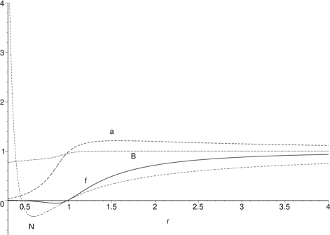
Figure 1: Solution for reduced theory (23) with $c^{\prime}_{1}=0.051$ and $c^{\prime}_{2}=0.116$, determined by data $N_{1}=-1$ and $a_{2}=-0.1$ at spatial infinity. There is both an outer and inner metric horizon where $N$ vanishes, but $f$ does not decrease enough to reach a spin-0 horizon. The functions $N$ and $f$ go to zero slightly inside $r=1$ which would be the horizon radius of the corresponding Schwarzschild solution. As $a_{2}$ increases the minimum of $f(r)$ decreases until the solution acquires a spin-0 horizon, where is it generically singular.

shows the behavior of $N$, $B$, and $a$ for $N_{1}=-1$ and $a_{2}=-0.1$. In this case there are “outer” and “inner” metric horizons where $N=0$, but $f(r)$ does not reach as low as $-0.158$, which is required by (33) in this case for a spin-0 horizon. For values of $a_{2}<-0.1$ the minimum value of $N$ shifts upward and eventually $N$ never reaches zero, i.e. the metric horizon disappears. On the other hand, for $a_{2}>-0.1$ the minimum value of $f$ decreases until the spin-0 horizon is reached. At this point $a^{\prime}$ goes to negative infinity, $N^{\prime}$ blows up to positive infinity, and there is a curvature singularity. In contrast, note that in Figure 1 $a^{\prime}(r)$ has a maximum value while $N^{\prime}(r)$ goes to negative infinity. This suggests that at some special value of $a_{2}$ there is a transition were the concavity of $a^{\prime}(r)$ and $N^{\prime}(r)$ changes and the derivatives are finite at a spin-0 horizon. Regularity at the spin-0 horizon seems thus to impose one condition on the asymptotic values $N_{1}$ and $a_{2}$.

In the negative mass case one might expect only solutions analogous to negative mass Schwarzschild, with $N$ increasing from 1 at spatial infinity and no spin-0 or metric horizon. While the solution does take this form for all $a_{2}$ in the theory with $c^{\prime}_{1}=0.051$, $c^{\prime}_{2}=0.116$, for other values of $c^{\prime}_{1,2}$ there are ranges of $a_{2}$ where $N$ increases from 1 at infinity, but then decreases to a metric horizon at finite $r$, and all the functions and their derivatives are regular until $f(r)$ reaches the value less than zero required for a spin-0 horizon. This peculiar behavior of a negative mass solution with metric and spin-0 horizons remains to be studied more closely. In particular, it is not clear whether a negative mass solution with a regular spin-0 horizon could exist.

5 Black holes with regular spin-0 horizons

In this section we discuss the behavior of black hole solutions possessing regular spin-0 horizons. Rather than imposing regularity at the spin-0 horizon by the shooting method integrating in from infinity, we instead expand the field equations in a power series about a non-singular spin-0 horizon.

5.1 Horizon expansion

Due to the complexity of the field equations and their singular nature at the horizon, we were unable to implement the power series solution about a spin-0 horizon in the generic reduced theory (23) (even with computer aided algebra). It might be possible to obtain the perturbative solution by a more well-adapted method, but instead we simplified the computation by making a field redefinition to a new metric for which the spin-0 and metric horizons coincide. Starting from an arbitrary set of coefficients $c_{i}$, this is implemented by the choice $\sigma=s_{0}^{2}$ in (14), after which we have $s_{0}=1$ without loss of generality in the theory. As before we can also then exploit spherical symmetry to absorb $c_{4}$ by making the replacements (7), which do not disrupt the coincidence of the spin-0 and metric horizons since this is just a re-expression of the same Lagrangian without changing the field variables . This reduces the distinct parameter space to just ($c_{1}$,$c_{3}$) (omitting the prime in the notation for $c_{1,3}$). After this field redefinition the coefficient $c_{2}$ is given by

$$c_{2}=\frac{-2c_{3}-c_{1}^{3}-2c_{3}c_{1}^{2}-c_{1}c_{3}^{2}}{2-4c_{1}+3c_{1}^{2}+3c_{3}c_{1}}.$$ (35)

A further simplification of the equations is achieved by trading the metric function $N$ for the combination of metric and aether functions $f=Na^{2}$. We have no insight into why this simplifies the expansion of the field equations about the common metric and spin-0 horizon at $N=0=f$, although as stated above the combination $Na^{2}$ is invariant under a rescaling of the $v$ coordinate. The field equations in this set of field variables involve $a$, $a^{\prime}$, $a^{\prime\prime}$, $f$, $f^{\prime}$, $f^{\prime\prime}$, $B$, and $B^{\prime}$. At the horizon $f(r)$ vanishes linearly, $f(r)=f^{\prime}(r_{0})(r-r_{0})+\cdots$ By a constant rescaling of $v$ we can furthermore set $B(r_{h})$ equal to 1. Using this along with (28) and (29) the field equations can be expanded and solved order by order for the coefficients of the power series.

Solving the field equations for this theory as algebraic equations for the expansion coefficients we find that at zeroth order in $(r-r_{h})$ the quantities $a(r_{h})$, $a^{\prime}(r_{h})$, $a^{\prime\prime}(r_{h})$, and $f^{\prime\prime}(r_{h})$ are determined by free parameters $r_{h}$, $f^{\prime}(r_{h})$, $B^{\prime}(r_{h})$. We succeeded in solving the equations to the next order in $(r-r_{h})$ only in the special cases $c_{3}=0$, $c_{3}=c_{1}$, and $c_{3}=-c_{1}$. In these cases we find that $B^{\prime}(r_{h})$ is determined by $r_{h}$ and $f^{\prime}(r_{h})$. Hence, consistent with the expectation of the previous section, there is a two-parameter family of local solutions around the regular spin-0 horizon. These solutions are generically not asymptotically flat.

5.2 Asymptotically flat black holes

To produce asymptotically flat solutions we numerically integrate outward, starting with the horizon data and matching onto (30), (31), and (32) by tuning $f^{\prime}(r_{h})$ until $f(r)$ is constant and equal to 1 at very large $r$ values. The asymptotic flatness boundary condition at infinity thus reduces the number of free parameters to one, namely the horizon radius itself. Solutions with different horizon radii are trivially related. Since $r_{h}$ is a singular point of the ODE’s, it is necessary to start the integration with initial data at some small positive value of $r-r_{h}$. We used the series solution determined by a given $r_{h}$ and $f^{\prime}(r_{h})$ to generate this initial data. To examine the solution inside the horizon, we numerically integrated inward, starting at a small negative value of $r-r_{h}$ with data generated by the same series solution.

Here we will discuss the properties of the solutions for the $c_{3}=0$ theory only, whose behavior is typical of the three special cases $c_{3}=0,\pm c_{1}$. Figure 2 displays the solution for $c_{1}=0.3$, $c_{2}=-.025$, $c_{3}=c_{4}=0$, together with $S(r)=1-2/r$, the Schwarzschild version of $N(r)$ with the same mass.

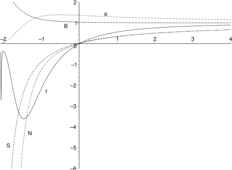
Figure 2: Plots of $f$, $N$, $B$, $a$, and $S$ (the Schwarzschild version of $N$) vs. $z=r-r_{h}$ for $c_{1}=0.3$, in units with $r_{0}=2$. The horizon radius is $r_{h}\approx 2.07$ for the ae-theory black hole, so $S=0$ at $z\approx-0.07$. The solutions agree closely outside the horizon. Deviations are noticeable near the horizon and become significant in the interior, where $N$ blows up more rapidly. Near the singularity $f$ begins to oscillate rapidly.

For this plot we use the scaling freedom of $v$ to convert the numerical solution to a “gauge” where the metric functions and $v$ component of the aether are all equal to 1 at infinity. The two metric functions $B(r)$ and $N(r)$ in GR and ae-theory are in very close agreement outside the horizon, while inside they differ noticeably.

5.2.1 Black hole mass

The ADM mass $M_{ADM}$ of an asymptotically flat spacetime whose asymptotic metric takes the Schwarzschild form at $O(1/r)$ is directly determined by the coefficient $r_{0}=2GM_{ADM}$ of the $O(1/r)$ part of $g_{tt}$. In ae-theory the relation between $M_{ADM}$ and the total energy $E$ of the spacetime is $GM_{ADM}=G_{N}E$ [17, 9], where $G_{N}=G/(1-c_{14}/2)$ is the Newton constant appearing in the force law between two weakly gravitating masses [12]. We shall refer to the quantity $r_{0}/2$ with dimensions of length as the “mass” in what follows, and denote it by $M$. For a Schwarzschild black hole in GR, $r_{0}$ is equal to the horizon radius $r_{h}$. In ae-theory the ratio $r_{0}/r_{h}$ is a constant (since there is only one length scale) determined by the coupling coefficients $c_{i}$.

The EF line element (24) transforms to Schwarzschild form

$$ds^{2}=N\,dt^{2}-(B^{2}/N)\,dr^{2}-r^{2}d\Omega^{2}$$ (36)

with time coordinate $t$ defined by $dt=dv-(B/N)dr$. The asymptotic form of $B$ (31) shows that $B=1+O(1/r^{2})$, so up through $O(1/r)$ the line element (36) has the standard asymptotic form if $N$ and $B$ are normalized to 1 at infinity. In generating an asymptotically flat numerical solution we fixed the scale freedom of the $v$ coordinate by imposing $B(r_{h})=1$ at the horizon however, so the asymptotic form of $N$ is $N_{\infty}+N_{1}/r+O(1/r^{2})$. The mass is given by $M=r_{0}/2=N_{1}/2N_{\infty}$, which can be extracted from the numerical solution at large $r$.

5.2.2 Horizons

The solution displayed in Figure 2 has metric and spin-0 horizons at $z=0$, but how about spin-1 and spin-2 horizons? Is the fastest speed actually trapped? The condition for a horizon corresponding to a speed $s_{0}$ is given in (33). As the speed approaches infinity the horizon value of $f$ approaches $-1$ from above. In Figure 2 (and for all values of $c_{1}$ that we studied up to $0.7$), the minimum value of $f(r)$ is less than $-1$, which is sufficient to trap any wave mode. The fact that $f(r)$ curves back to being greater than $-1$ indicates that an inner horizon might exist for some wave modes in certain parameter ranges of $c_{i}$.

In the theory under discussion we have $c_{3}=c_{4}=0$ and $c_{2}=-c_{1}^{3}/(2-4c_{1}+3c_{1}^{2})$, so the squared mode speeds in (1) are given by $1/(1-c_{1})$ for spin-2 and $(1-c_{1}/2)/(1-c_{1})$ for spin-1. With $0<c_{1}<1$ both of these are greater than 1, and the spin-2 speed is the highest. In the particular case shown in the figure, the spin-1 speed is $1.10$ and the spin-2 speed is $1.20$, which correspond to horizons at $f=-0.049$ and $f=-0.089$ respectively, which do not seem to be reached a second time.

5.2.3 Oscillations

A notable aspect of the black hole interior displayed in Figure 2 is the oscillation in $f$. The function $h=Ba$ also oscillates in a similar manner, but is 180 degrees out of phase. In addition, there are related oscillations in the curvature scalar and aether congruence behavior discussed below. These oscillations are reminiscent of the interior behavior found in Einstein-Yang-Mills black holes [18], where the metric functions and derivative of the Yang-Mills potential oscillate an infinite number of times before the singularity.

While $N$ decreases monotonically and $B$ increases monotonically, $a$ goes to zero, so the oscillations of $Na^{2}$ and $Ba$ arise because of variations in the magnitude of their derivatives. Since the oscillations inside $z=-2$ are not clearly visible in Figure 2 a zoomed in graph of $f(z)$ is provided in Figure 3.

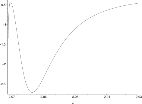
Figure 3: Oscillations of $f=Na^{2}$ near the singularity inside the black hole solution shown in figure 2, plotted vs. $z=r-r_{h}$ in units with $M=1$.

From this graph it is clear that $f$ smoothly turns over at least once more before the singularity. Although the number of oscillations before the singularity appears finite, it is possible that the numerical integration employed is not capable of resolving additional or even infinitely more oscillations. More information may be obtained in the future by improved numeric methods or analytic methods around $r=0$.

5.2.4 Curvature singularity

There appears to be a spacelike curvature singularity at or near $r=0$, as in the Schwarzschild solution of GR. In Figure 2, the approach of $N$ to negative infinity near $r=0$ suggests a singularity. In Figure 4 the logarithm of the Kretschmann scalar $K=R_{abcd}R^{abcd}$ is plotted vs. $\ln r$ for the ae-theory solution together with its value in the corresponding Schwarzschild solution with the same mass. In the latter case $K=48/r^{6}$ in units with $M=1$, so $\log K=-6\ln r+\ln 48$. The rate $d\ln K/d\ln r$ for the ae-theory solution seems to alternate between roughly $-6$ and $-4.5$. The location of the transitions may be correlated with the oscillations discussed above.

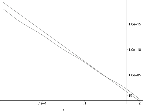
Figure 4: Plot of $\ln R_{abcd}R^{abcd}$ vs. $\ln r$ for $c_{1}=0.3$ ae-theory black hole (wiggly curve) and Schwarzschild black hole (stright line) of the same mass, in units with $M=1$. $r$ is plotted on a logarithmic scale. The slope for the GR case is $-6$, while for the ae-theory case it alternates between roughly $-6$ and $-4.5$.

The location of the singularity seems to be at $r=0$ for all the values of $c_{1}$, although our numerical solutions do not permit a determination of the exact location.

5.2.5 Aether congruence

The aether field defines a congruence of radial timelike curves at rest at infinity and flowing into the black hole. It is interesting to compare this with the static frame and with the congruence of freely falling radial geodesics with 4-velocity $v^{a}$ that are also at rest at infinity. Being unit vector fields, at each point $u^{a}$ and $v^{a}$ can be fully characterized by their Killing energy, i.e. their inner product with the Killing vector. The free-fall congruence has a conserved energy that is equal to one if the Killing vector is normalized to one at infinity. The aether does not fall as quickly outside the black hole. In fact it remains rather aligned with the Killing vector up until quite close to the horizon.

To characterize and contrast the free-fall and aether congruences we plot in Figure 5 the derivative $dr/d\tau$ of radius with respect to proper time along each congruence. Let us call this the quantity the “proper velocity”.

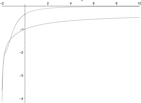
Figure 5: Radial proper velocity $dr/d\tau$ of free-fall (lower, solid curve) and aether (upper, dashed curve) vs. $z=r-r_{h}$, in units with $M=1$, for $c_{1}=0.3$. In contrast to the free-falling geodesics, the aether does not begin to fall significantly inward until close to the horizon.

The aether and free-fall are both at rest at infinity, but only as the horizon is approached is the aether finally pulled away from the Killing direction. As close as $r=3r_{h}$ ($z\approx 4$), the proper velocity of the aether is still about fifteen times smaller than that of free-fall. Inside the horizon the aether proper velocity is equal to the free-fall one around $z=-1.3$, but the 4-velocities do not agree there. The aether is still going inward faster, but its proper time is “running slower” so it can have the same proper velocity.

To compare the aether and free-fall motions inside the horizon we plot in Figure 6 the inward 3-velocity of the aether with respect to the free-falling frame.

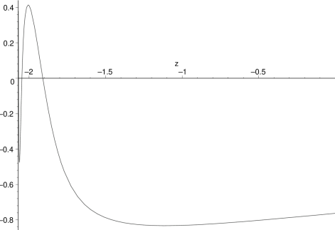
Figure 6: Inward 3-velocity of the aether relative to free-fall inside the horizon for $c_{1}=0.3$. The velocity is initially negative and the aether lags behind the free-fall. Near the singularity the velocity oscillates between between faster and slower than free-fall.

The relative velocity is initially negative, meaning that the aether is not falling in as fast as the the free-fall frame. It is clear from this plot at around $z=-1.3$ the aether still lags well behind free-fall. However, around $z=-1.9$ the relative velocity is zero, and after that it oscillates a couple of times (at least) before reaching the singularity.

5.2.6 Surface gravity and the first law of black hole mechanics

The laws of black hole mechanics have been shown to apply to a wide class of generally covariant metric theories of gravity coupled to matter [19]. There appears to be no straightforward extension of the first law and the concept of black hole entropy to ae-theory however [17], a difficulty that is tied to the fact that there is no smooth extension of the aether to the bifurcation surface of the Killing horizon. Moreover, it is not clear to which horizon the law should apply, in a theory with multiple characteristic surfaces. For example, in the solutions considered in this section, the spin-2 horizon is inside the spin-1 horizon which is inside the joint spin-0 and metric horizon. One might imagine that the relevant horizon is always the Killing horizon, but recall that by a field redefinition we can make any one of these horizons be the Killing horizon. We shall not try to shed any light on these puzzling issues here. Rather, we just briefly examine the variational relation between mass, surface gravity and area of the spin-0 horizon, for possible future use.

The first law of black hole mechanics for spherically symmetric neutral black holes in GR takes the form

$$\delta M=\alpha\frac{\kappa\delta A}{8\pi G},$$ (37)

where $A=4\pi r_{h}^{2}$ is the horizon area, $\kappa$ is the surface gravity, and $\alpha=1$. By dimensional analysis such a variational relation must also hold in ae-theory, with some value for the dimensionless constant $\alpha$ that depends on the dimensionless coupling coefficients $c_{i}$. Presumably for $M$ we should put the total energy $E$ of the spacetime, and for $``G"$ we should put the Newton constant $G_{N}$ governing the attractive force between distant bodies. Alternatively one might use the ADM mass $M_{ADM}$ and the constant $G$ appearing in the ae-theory action (3). As discussed in section 5.2.1, $GM_{ADM}=G_{N}E=r_{0}/2$, so these two choices actually yield identical “first laws”. If we express the mass and area in terms of $r_{0}$ and $r_{h}$ respectively, (37) thus becomes

$$\delta r_{0}=2\alpha\kappa r_{h}\delta r_{h}.$$ (38)

As pointed out in section 5.2.1, $r_{0}$ and $r_{h}$ are proportional, so we infer that $\alpha$ is determined by the dimensionless combination

$$\alpha=\frac{r_{0}}{2\kappa r_{h}^{2}},$$ (39)

which depends on the coefficients $c_{i}$ defining the theory.

5.2.7 Black hole properties for different values of $c_{1}$

Various properties of the black hole solutions for different values of $c_{1}$ are displayed in Table 1. The other coupling coefficients have the values $c_{3}=c_{4}=0$ and $c_{2}$ is given by (35). For each $c_{1}$ there is a one-parameter family of black hole solutions with regular spin-0 horizon, labeled by horizon radius. For the values in the table we compare black holes with the same horizon radius, and adopt units with $r_{h}=1$. The Killing vector which enters the definition of $\kappa$ and $\alpha$ is normalized to unity at spatial infinity.

Table 1: Properties of black hole solutions for several $c_{1}$ values, in units with $r_{h}=1$.

• $c_{1}$	$f^{\prime}(r_{h})$	$\gamma=u^{a}v_{a}$	$r_{0}$	$\kappa$	$\alpha$
  0.1	2.096	1.619	0.990	0.507	0.976
  0.2	2.072	1.608	0.979	0.517	0.947
  0.3	2.039	1.592	0.966	0.528	0.914
  0.4	1.997	1.568	0.951	0.543	0.876
  0.5	1.941	1.535	0.933	0.562	0.830
  0.6	1.867	1.490	0.911	0.588	0.787
  0.7	1.767	1.429	0.881	0.625	0.704

The values of $f^{\prime}(r_{h})$ that yield asymptotically flat solutions for different choices of $c_{1}$ are displayed in the 2nd column. These values decrease as $c_{1}$ grows. For $c_{1}=0.8$ and larger we could not find a $f^{\prime}(r_{h})$ that yielded an asymptotically flat solution. The third column shows the gamma factor between the aether and free-fall velocity at the horizon. The fourth column shows $r_{0}=2GM_{ADM}$. This is equal to $r_{h}$ for $c_{1}=0$ (a Schwarzschild black hole), and decreases by 12% as $c_{i}$ increases up to 0.7. Conversely, for a given mass the black hole horizon is larger for larger $c_{1}$. The fifth column shows the surface gravity, which for $c_{1}=0$ is $1/2r_{h}$ and increases by 25% as $c_{1}$ increases up to $0.7$. The last column is the dimensionless ratio (39) appearing in the first law (37), which is unity for $c_{1}=0$ and decreases by 30% as $c_{1}$ increases to 0.7.

6 Discussion

In this paper we considered the meaning of a black hole in Einstein-Aether theory, arguing that the fastest wave mode must be trapped if the configuration is to qualify as a causal black hole. Regularity at the spin-0 horizon was identified as a key property of black holes in ae-theory. It was found that, for generic values of the coupling constants $c_{i}$, regularity at a metric horizon imposes no restrictions on spherically symmetric, static local solutions but regularity at a spin-0 horizon imposes one condition. At least for a class of coupling constants, there is a one parameter family of asymptotically flat black hole solutions with all horizons (metric and spin-0,1,2) regular.

From an astrophysical point of view an essential question is what happens when matter collapses. It is a plausible conjecture that nonsingular spherically symmetric initial data will evolve to one of the regular black holes whose existence has been demonstrated here, but this has certainly not been shown. It would be very interesting to answer this question by numerical evolution of the time-dependent field equations. To do so, one could add scalar matter to form a collapsing pulse, but this is likely not necessary since the aether itself has a spherically symmetric radial tilt mode that can serve the purpose. This would correspond to formation of a black hole by an imploding spherical aether wave.

We examined several properties of regular black hole solutions for a special class of coupling coefficients defining the ae-theory. A complete classification of the solutions for different coefficients remains an open research problem, as does the study of non-black hole solutions and negative mass solutions, which strangely enough could include black holes. Oscillating behavior approaching the internal singularity has been identified, but not studied in detail. Finally, only the static, spherically symmetric case was examined; the question of rotating black hole solutions remains untouched.

References

References

- [1] Eling C, Jacobson T and Mattingly D 2006 Einstein-aether theory Deserfest ed J Liu, M J Duff, K Stelle, and R P Woodard (Singapore: World Scientific) (Preprint gr-qc/0410001).
- [2] Kostelecky V A 2004 Gravity, Lorentz violation, and the standard model Phys. Rev. D 69 105009 (Preprint hep-th/0312310).
- [3] Bailey Q G and Kostelecky V A 2006 Signals for Lorentz violation in post-Newtonian gravity Phys. Rev. D, to appear (Preprint gr-qc/0603030).
- [4] Eling C and Jacobson T 2004 Static post-Newtonian equivalence of GR and gravity with a dynamical preferred frame Phys. Rev. D 69 064005 (Preprint gr-qc/0310044).
- [5] Graesser M L, Jenkins A and Wise M B 2005 Spontaneous Lorentz violation and the long-range gravitational preferred-frame effect Phys. Lett. B 613 5 (Preprint hep-th/0501223).
- [6] Foster B Z and Jacobson T 2006 Post-Newtonian parameters and constraints on Einstein-aether theory Phys. Rev. D 73, 064015 (Preprint gr-qc/0509083).
- [7] Jacobson T and Mattingly D 2004 Einstein-aether waves Phys. Rev. D 70 024003 (Preprint gr-qc/0402005).
- [8] Lim E A 2005 Can we see Lorentz-violating vector fields in the CMB? Phys. Rev. D71 063504 (Preprint astro-ph/0407437)
- [9] Eling C 2006 Energy in the Einstein-aether theory Phys. Rev. D 73 084026 (Preprint gr-qc/0507059).
- [10] Foster B Z 2006 Radiation damping in Einstein-aether theory Phys. Rev. D 73 104012 (Preprint gr-qc/0602004).
- [11] Elliott J W, Moore G D and Stoica H 2005 Constraining the new aether: Gravitational Cherenkov radiation JHEP 0508, 066 (Preprint hep-ph/0505211).
- [12] Carroll S M and Lim E A Lorentz-violating vector fields slow the universe down 2004 Phys. Rev. D 70 123525 (Preprint hep-th/0407149).
- [13] Eling C and Jacobson T 2006 Spherical Solutions in Einstein-Aether Theory: Static Aether and Stars Class. Quantum Grav. , to appear (Preprint gr-qc/0603058).
- [14] Courant R and Hilbert D 1962 Methods of Mathematical Physics, (New York: Interscience Publishers).
- [15] Racz I and Wald R M 1996 Global extensions of space-times describing asymptotic final states of black holes Class. Quantum Grav. 13 539 (Preprint gr-qc/9507055).
- [16] Foster B Z 2005 Metric redefinitions in Einstein-aether theory Phys. Rev. D 72 044017 (Preprint gr-qc/0502066).
- [17] Foster B Z 2006 Noether charges and black hole mechanics in Einstein-aether theory Phys. Rev. D 73 024005 (Preprint gr-qc/0509121).
- [18] Donets E E, Galtsov D V and Zotov M Y 1997 Internal structure of Einstein Yang-Mills black holes Phys. Rev. D 56 3459 (Preprint gr-qc/9612067).
- [19] Wald R M 2001 The thermodynamics of black holes Living Rev. Rel. 4 6 (Preprint gr-qc/9912119).