Weaker Gravity at Submillimetre Scales in Braneworld Models

Abstract

Braneworld models typically predict gravity to grow stronger at short distances. In this paper, we consider braneworlds with two types of additional curvature couplings, a Gauss-Bonnet (GB) term in the bulk, and an Einstein-Hilbert (EH) term on the brane. In the regime where these terms are dominant over the bulk EH term, linearized gravity becomes weaker at short distances on the brane. In both models, the weakening of gravity is tied to the presence of ghosts in the graviton mass spectrum. We find that the ordinary coupling of matter to gravity is recovered at low energies/long wavelengths on the brane. We give some implications for cosmology and show its compatibility with observations. We also discuss the stability of compact stars.

I Introduction

Current measurements of gravity do not deviate from Newton’s law at distances greater than $0.2$mm Hoyle:2000cv , leaving open the possibility that gravity might be modified at shorter length scales. The potential observation that gravity is weaker at small distances would be a serious challenge to current high energy theories, forcing us to develop unconventional ideas. In this spirit, we shall consider a class of examples framed within braneworld models where gravity can be weaker than Newton’s law at small distances. For a review on theoretical models predicting a deviation from Newton’s inverse-square law, and on experimental tests, see Ref. Adelberger:2003zx .

In braneworld scenarios, gravity on the brane is expected to be modified at distances of order of the size of the extra-dimension ADD , or the bulk curvature scale Randall:1999vf . The measurement of gravity at submillimeter scales might therefore provide a way to test braneworld scenarios. In particular, the Randall-Sundrum (RS) model Randall:1999vf , gives rise to a modification of gravity which appears stronger at short distances Garriga:1999yh ; Callin:2004py . This is due to the presence of massive Kaluza-Klein (KK) modes which contribute negatively to the gravitational potential on the brane. In any braneworld model, the presence of the KK modes of the graviton will typically modify the gravitational potential generated by a source of mass $M$ in the following way

$$V(r)=-MG_{4}\left(\frac{1}{r}+\int_{0}^{\infty}\mathrm{d}m\,\frac{e^{-mr}}{r}\rho(m)\right),$$ (1)

a result which follows from the Kallen-Lehmann spectral representation of the propagator. Here $\rho(m)$ measures the influence of the KK modes of mass $m$ on the brane . For gravity to appear weaker in any regime, the spectral density $\rho(m)$ should be negative for some range of $m$. However, unitarity (absence of ghosts) usually requires $\rho(m)\geq 0$.

This result is generic to many modifications of gravity, for instance if there are additional gravitational strength interactions mediated by other massive spin-0 or spin-2 particles, (see for instance Ref. Callin:2005wi ). However, there are exceptions, for instance it has been proposed that the graviton is a composite particle, ie. has some finite size Sundrum:2003jq ; Sundrum:2003tb , and that the force of gravity would be naturally cut of at this size. In Ref. Biswas:2005qr , higher derivative modifications to the gravitational action were considered making it ‘asymptotically safe’, also providing a cutoff to the force of gravity at small distances. A less radical proposal would be an additional weakening from the exchange of massive spin-1 bosons which would give a repulsive Yukawa modification to Newton’s law Adelberger:2003zx . These new gauge fields could be propagating in the bulk of any typical braneworld scenario, and could mediate a force of the same order of magnitude as gravity. Such gauge fields would necessarily violate the Equivalence Principle and the gauge coupling to ordinary matter would be strongly constrained by experiments Smith:1999cr .

In the examples that follow we shall consider the possibility that $\rho(m)<0$, signalling the presence of ghosts. Ghosts in a theory are typically a problem for two reasons: Firstly they suggest the presence of a classical instability, the significance of which needs to be addressed in the context of a specific model. Secondly they signal the breakdown of unitarity, or of a quantum instability due to their carrying negative energy, see Ref. Cline:2003gs . However, if conventional gravity is recovered at low energies, as will be the case in our examples, unitarity is expected to be restored in that limit. In what follows we shall simply assume that the usual notions of quantum field theory do not apply to gravitation at least at submillimetre scales, and that some unusual notion of quantum gravity resolves this issue Hawking:2001yt .

In this work, we consider the potential corrections arising on a brane embedded in a five-dimensional space-time. Although the preceding argument suggests the presence of instabilities, we show how these models are nonetheless classically viable, and are consistent with cosmological observations.

As a first example, we consider the extension of the RS model to the case when GB terms are present in the bulk Wheeler:1985qd ; Neupane:2001st ; Deruelle:2003tz ; Maeda:2003vq ; Neupane:2001kd ; Cho:2001nf ; Bronnikov:2006jy . In this work, we explore the possibility that these terms have a contribution of the same order of magnitude as the EH term. Such a regime is not usually taken into account in the literature, where the GB terms are usually thought to arise from quantum/string corrections (see Ref. Boulware:1985wk ) and are therefore small. In a five-dimensional spacetime, the GB terms are the unique functions of the metric that do not alter the Cauchy problem Meissner:2000dy . This implies that there are no new degrees of freedom and the equations of motion have no higher than second order time derivatives Deruelle:2003ck ; Kakushadze:2001bd . Once the GB terms are important, nothing allows us a priori to ignore the higher-order corrections terms. We shall however assume a large hierarchy between the GB term and other higher order corrections. Hierarchy problems are common to gravity, naively one would expect the cosmological constant to be of order of magnitude $10^{120}$ times more than its actual observed value. It is not clear then that our usual notions of naturalness apply to gravity, and we will therefore explore this possibility in what follows.

We find in this example that the contribution from the KK corrections actually reverses sign, leading to weaker gravity at short distances. The expected instability associated with this mechanism can be understood when we study the response to bulk matter. In this regime, the gravity part in the five-dimensional action reverses sign, leading to a “wrong” coupling between gravity and bulk matter. There is however no instability associated with matter on the brane, and the theory on the brane is stable, at least at the classical level.

Motivated by this result, we consider an alternative scenario, where the gravitational response to matter on the bulk will be stable. We introduce a negative EH term into the brane action and imagine that matter on the brane couples with the “wrong sign” action. In that case gravity will respond the correct way to bulk matter far away from the brane, and the correct way to any matter confined on the brane. The theory is therefore stable, at least classically and the theory on the brane presents all the general features necessary to explain the cosmological behaviour of our Universe. Gravity will however appear weaker on short scales.

This work is organized as follows. We start by reviewing the RS model in presence of GB terms in section II. After presenting the background spacetime behaviour, we study the response of gravity to a static source on the brane and show that gravity appears weaker at short-distances. We then discuss the implications for cosmology, and show that at low-energy the four-dimensional behaviour is recovered. The stability of this model is then studied and the response to bulk matter is shown to be unstable. We then focus on an alternative model in section III, where no GB terms are present in the bulk, but instead a EH term on the brane action which we take with a negative sign. The consequences for cosmology are explored and the gravity is shown to be weaker at short scales. We show that both the weak and null energy conditions are satisfied for the effective energy density provided it is satisfied by the matter field confined on the brane. Finally we present other physical implications of these two models in section IV. In particular we discuss the implications of weaker gravity on the stability of massive stars. For weaker gravity at short distances, we show that the stability of compact stars is improved.

In what follows, we use the index notation that Roman indices are fully five-dimensional, while Greek indices are four dimensional, labeling the transverse $x^{\mu}$ direction along the brane. Roman fonts $\mathrm{R},\mathrm{G}$, designate quantities with respect to the five-dimensional metric, whereas normal fonts $R,G$ designate quantities evaluated with respect to the induced metric on the brane.

II Weaker gravity from GB braneworld model

II.1 GB braneworld model

Our starting point is the five-dimensional action

$$S^{(\text{5d})}=\frac{1}{2\kappa_{5}^{2}}\int\mathrm{d}^{5}x\sqrt{-g}\left[\mathrm{R}-2\Lambda+\frac{\beta\ell^{2}}{4}\,\mathcal{R}_{2}\right]+S^{(\text{4d})}_{b},$$ (2)

where $\Lambda$ is the bulk cosmological constant. In general $\Lambda$ is considered to be negative so that the bulk vacuum geometry is Anti-de Sitter (AdS), but as we shall see this condition can be relaxed for some values of the coefficient $\beta$ of the GB terms $\mathcal{R}_{2}$. The AdS length scale of our chosen vacuum is denoted as $\ell$, and the GB term $\mathcal{R}_{2}$ is the trace of

$$\mathcal{R}^{\,A}_{2\,B} = \mathrm{R}\,\mathrm{R}^{A}_{B}-2\,\mathrm{R}^{A}_{C}\,\mathrm{R}^{C}_{B}-2\mathrm{R}^{CD}\,\mathrm{R}^{A}_{\ \ CBD}$$

$$+\mathrm{R}^{A}_{\ \ DEF}\,\mathrm{R}_{B}^{\ \ DEF},$$

where $\mathrm{R}^{A}_{\ \ BCD}$ is the five-dimensional Riemann tensor. Finally the term $S^{(\text{4d})}_{b}$ in (2) is the four dimensional action for the brane:

$$S^{(\text{4d})}_{b}=\int_{\text{brane}}\mathrm{d}^{4}x\sqrt{-q}\left(Q+\mathcal{L}_{m}-\lambda\right),$$ (4)

where $Q$ gives us the generalization of the Gibbon-Hawking’s boundary terms Gibbons:1976ue ; Myers:1987yn :

$$Q=2K+\beta\ell^{2}\left(J-2G^{\mu}_{\nu}K^{\nu}_{\mu}\right),$$ (5)

$K^{\mu}_{\,\nu}$ being the extrinsic curvature on the brane, $G^{\mu}_{\,\nu}$ being the Einstein tensor on the brane and

$$J^{\mu}_{\,\nu}=-\frac{2}{3}K^{\mu}_{\alpha}K^{\alpha}_{\beta}K^{\beta}_{\nu}+\frac{2}{3}K\,K^{\mu}_{\alpha}K^{\alpha}_{\nu}+\frac{1}{3}K^{\mu}_{\,\nu}(K^{\alpha}_{\beta}K^{\beta}_{\alpha}-K^{2}).$$ (6)

In the brane action, we separate the brane tension $\lambda$ from the brane matter fields Lagrangian $\mathcal{L}_{m}$.

In the five-dimensional bulk, the Einstein equations are

$$\mathcal{G}^{A}_{B}=\mathrm{G}^{A}_{B}+\frac{1}{2}\beta\ell^{2}\mathcal{R}^{\,A}_{2\,B}-\frac{1}{8}\beta\ell^{2}\mathcal{R}_{2}\,\delta^{A}_{B}+\Lambda\delta^{A}_{B}=0.$$ (7)

For pedagogical reasons, let us consider the case that the bulk is AdS with length scale $\ell$, so that the metric is

$$\mathrm{d}s^{2}=\mathrm{d}y^{2}+e^{-2y/\ell}\eta_{\mu\nu}\mathrm{d}x^{\mu}\mathrm{d}x^{\nu},$$ (8)

in flat slicing. Then the Einstein equation (7) implies the relation between $\beta$, $\ell$ and $\Lambda$.

$$\mathcal{G}^{A}_{B}=\frac{1}{\ell^{2}}\left(6-3\beta+\ell^{2}\Lambda\right)\delta^{A}_{B}=0.$$ (9)

The AdS length scale is therefore related to the bulk cosmological constant

$$\Lambda=-\frac{6}{\ell^{2}}+\frac{3\beta}{\ell^{2}}.$$ (10)

In the absence of GB terms, ($\beta=0$), we recover the usual canonical RS tuning Randall:1999vf . In the presence of GB terms, the bulk can hold an AdS solution without the presence of any bulk cosmological constant if $\beta$ takes the specific value $\beta=2$, as already pointed out in Deser:1987uk ; Deser:1989jm ; Crisostomo:2000bb ; Corradini:2004qr . There is an AdS solution in the presence of a positive bulk cosmological constant when $\beta>2$. In this paper we explore the possibility of having relatively large GB terms, ie. $\beta\gtrsim 1$, but not necessarily $\beta>2$.

The boundary conditions on the brane is given by the analogue of the Israël matching conditions Israel:1966rt in presence of GB terms Myers:1987yn ; Davis:2002gn :

$$K^{\mu}_{\nu}+\frac{\beta\ell^{2}}{3}\left(\frac{9}{2}J^{\mu}_{\nu}-J\delta^{\mu}_{\nu}-3P^{\mu}_{\ \ \alpha\nu\beta}K^{\alpha\beta}+P^{\rho}_{\ \ \alpha\rho\beta}K^{\alpha\beta}\delta^{\mu}_{\,\nu}\right)$$

$$=-\frac{\kappa_{5}^{2}}{6}\lambda\delta^{\mu}_{\,\nu}-\frac{\kappa_{5}^{2}}{2}\left(T^{\mu}_{\,\nu}-\frac{1}{3}T\delta^{\mu}_{\,\nu}\right),\hskip 8.0pt$$ (11)

where

$$P^{\mu}_{\ \ \alpha\nu\beta} = \left(R^{\mu}_{\beta}q_{\alpha\nu}+R_{\alpha\nu}\delta^{\mu}_{\beta}-R_{\alpha\beta}\delta^{\mu}_{\nu}-R^{\mu}_{\,\nu}q_{\alpha\beta}\right)$$

$$+R^{\mu}_{\ \ \alpha\nu\beta}-\frac{1}{2}R\left(\delta^{\mu}_{\beta}q_{\alpha\nu}-q_{\alpha\beta}\delta^{\mu}_{\,\nu}\right),$$

$R^{\mu}_{\ \ \alpha\nu\beta}$ being the four-dimensional Riemann tensor induced on the brane. $T^{\mu}_{\,\nu}$ represents the four-dimensional stress-energy tensor associated with the matter fields confined on the brane $\mathcal{L}_{m}$.

As for the normal RS model, a brane moving through a pure AdS bulk will undergo a flat Friedmann-Robertson-Walker (FRW) expansion or contraction in the induced geometry. In this case the extrinsic curvature is $K^{i}_{j}=k\delta^{i}_{j}$, with $k=-\frac{1}{\ell}\sqrt{1+\ell^{2}H^{2}}$, $H$ being the Hubble parameter on the brane. We have as well $\frac{9}{2}J^{i}_{j}-J\delta^{i}_{j}=-k^{3}\delta^{i}_{j}$ and $-3P^{i}_{\ \ \alpha j\beta}K^{\alpha\beta}+P^{\rho}_{\ \ \alpha\rho\beta}K^{\alpha\beta}\delta^{i}_{j}=3H^{2}k\delta^{i}_{j}$. For spatially flat cosmologies the boundary condition (11) simplifies considerably:

$$k\left(1+\beta\ell^{2}\left(H^{2}-\frac{1}{3}k^{2}\right)\right)=-\frac{\kappa_{5}^{2}}{6}\left(\lambda+\rho\right),$$ (13)

$\rho$ being the energy density of the matter fields located on the brane. The modified Friedmann equation on the brane is therefore given by the solution of:

$$\sqrt{1+\ell^{2}H^{2}}\left[1+\frac{1}{3}\beta\left(-1+2\ell^{2}H^{2}\right)\right]=\frac{\ell\kappa_{5}^{2}}{6}\left(\lambda+\rho\right).$$ (14)

In particular, if the brane is empty for the background, $\rho=0$, and if the brane tension $\lambda$ is fine-tuned to its canonical value:

$$\lambda=\frac{6}{\kappa_{5}^{2}\,\ell}\left(1-\frac{1}{3}\beta\right),$$ (15)

the brane geometry becomes Minkowski spacetime ($H=0$) and the brane position remains static.

II.2 Linearized Gravity

We now consider linear perturbations around the background AdS geometry (8). In particular we will consider the brane (at $y=0$) to be empty for the background and to have a fine-tuned tension (15). We wish to study the metric perturbations sourced by matter confined on the brane with stress-energy tensor $T^{\mu}_{\,\nu}$. In RS gauge, the perturbed metric is:

$$\mathrm{d}s^{2}=\mathrm{d}y^{2}+\left(e^{-2|y|/\ell}\eta_{\mu\nu}+h_{\mu\nu}\right)\mathrm{d}x^{\mu}\mathrm{d}x^{\nu}$$ (16)

$$\text{with }h^{\mu}_{\mu}=0\text{ and }h^{\mu}_{\,\nu}{}_{,\mu}=0,$$

where indices are raised with respect to $\eta^{\mu\nu}$. In this gauge, the Einstein equation in the bulk is:

$$\left(1-\beta\right)\left[e^{2y/\ell}\Box+\partial_{y}^{2}-\frac{4}{\ell^{2}}\right]h^{\mu}_{\,\nu}=0,$$ (17)

where $\Box$ is the four-dimensional Laplacian in flat spacetime $\Box=\eta^{\mu\nu}\partial_{\mu\nu}$. In this gauge, the brane location is no longer fixed. We denote by $\delta y$ its deviation from $y=0$. We hence work in the Gaussian Normal (GN) gauge where the brane is “static”:

$$\bar{y} = y-\delta y(x^{\mu}),$$ (18)

$$\bar{x}^{\mu} = x^{\mu}-\left(\frac{\ell}{2}\left(e^{2y/\ell}-1\right)+\frac{2}{\ell\Box}\right)\eta^{\mu\nu}\delta y_{,\nu}.$$ (19)

In this new gauge, the perturbed metric is:

$$\bar{h}_{\mu\nu}(\bar{y}) = h_{\mu\nu}(y)-\ell(1-e^{-2y/\ell})\delta y_{,\mu\nu}$$

$$-\frac{2}{\ell}e^{-2y/\ell}\left(\eta_{\mu\nu}+\frac{2}{\Box}\partial_{\mu\nu}\right)\delta y.$$

We choose the remaining degrees of freedom in the GN gauge such that on the brane, the induced metric perturbation $\bar{h}_{\mu\nu}(0)$ is in de Donder gauge, hence $R^{\mu}_{\,\nu}=-\frac{1}{2}\Box\bar{h}^{\mu}_{\,\nu}(0)$. Using this relation, the boundary conditions becomes

$$\left(1-\beta\right)\delta K^{\mu}_{\,\nu}+\frac{\ell}{2}\beta\left(\Box\bar{h}^{\mu}_{\,\nu}-\frac{1}{6}\Box\bar{h}\delta^{\mu}_{\,\nu}\right)$$ (21)

$$=-\frac{\kappa_{5}^{2}}{2}\left(T^{\mu}_{\,\nu}-\frac{1}{3}T\delta^{\mu}_{\,\nu}\right),$$

where $\delta K^{\mu}_{\,\nu}=\frac{1}{2}\left[\partial_{y}+\frac{2}{\ell}\right]\bar{h}^{\mu}_{\,\nu}$. The boundary condition in RS gauge is summarized as:

$$\left(1-\beta\right)\left[\partial_{y}+\frac{2}{\ell}\right]h^{\mu}_{\,\nu}+\beta\ell\Box h^{\mu}_{\,\nu}=-\kappa_{5}^{2}\Sigma^{\mu}_{\,\nu},$$ (22)

where $\Sigma^{\mu}_{\,\nu}$ is a traceless and transverse tensor associated with the stress-energy tensor $T^{\mu}_{\,\nu}$:

$$\Sigma^{\mu}_{\,\nu}=T^{\mu}_{\,\nu}-\frac{1}{3}T\delta^{\mu}_{\,\nu}+\frac{1}{3\Box}\eta^{\mu\alpha}T_{,\alpha\nu},$$ (23)

and the perturbation of the brane location is $\delta y=-\frac{\kappa_{5}^{2}}{6\left(1+\beta\right)\Box}T$.

Solving the bulk Eq. of motion (17) with the boundary condition and the requirement that the perturbations die off at infinity, one has the solution:

$$h_{\mu\nu}(y)=\kappa_{5}^{2}\hat{F}\Sigma_{\mu\nu},$$ (24)

with

$$\hat{F}=\frac{1}{\sqrt{-\Box}}\frac{K_{2}\left(\sqrt{-\Box}\ell e^{y/\ell}\right)}{\left(1-\beta\right)K_{1}\left(\sqrt{-\Box}\ell\right)+\beta\sqrt{-\Box}\ell K_{2}\left(\sqrt{-\Box}\ell\right)},\hskip 5.0pt$$ (25)

where $K_{n}$ is the Bessel function. We may decompose this expression into the zero mode and the infinite tower of KK corrections for the induced metric perturbation on the brane:

$$\bar{h}_{\mu\nu}=-\frac{2\kappa_{5}^{2}}{\ell(1+\beta)\Box}\left(T_{\mu\nu}-\frac{1}{2}T\eta_{\mu\nu}\right)\hskip 90.0pt$$

$$+\frac{1-\beta}{1+\beta}\frac{K_{0}\left(\sqrt{-\Box}\ell\right)}{(1+\beta)K_{1}\left(\sqrt{-\Box}\ell\right)+\beta\sqrt{-\Box}\ell K_{0}\left(\sqrt{-\Box}\ell\right)}\frac{\kappa_{5}^{2}}{\sqrt{-\Box}}\Sigma_{\mu\nu}.$$ (26)

It is therefore clear from this result, that when $\beta<1$, the KK tower gives a positive correction to the zero mode which makes gravity stronger at short distances, whereas when $\beta>1$, the KK corrections will make gravity weaker at short distances. When $\beta=1$, linearized gravity appears purely four-dimensional on the brane (ie. without any KK correction) Crisostomo:2000bb .

To make this argument more precise, we consider a point-like source of mass $M$ on the brane: $T_{00}=M\delta(r)$, $T_{ij}=0$. This local source generates the following metric perturbations:

$$\bar{h}_{00} = \kappa_{5}^{2}M\left(\frac{1}{2}V_{0}+\frac{2}{3}V_{KK}\right)$$ (27)

$$\bar{h}_{ij} = \kappa_{5}^{2}M\left(\frac{1}{2}V_{0}+\frac{1}{3}V_{KK}\right)\delta_{ij}$$ (28)

where the contribution $V_{0}$ from the zero mode is

$$V_{0}=\int_{0}^{\infty}\mathrm{d}k\frac{k\sin kr}{2\pi^{2}r}\frac{2}{\ell(1+\beta)k^{2}}=\frac{1}{2\ell(1+\beta)\pi r},$$ (29)

and the contribution from the KK modes is (Cf. Appendix A and Eq. (66))

$$V_{KK}=\frac{1-\beta}{\left(1+\beta\right)^{2}}\frac{\ell}{4\pi r^{3}}+\mathcal{O}\left(\ell^{3}/r^{5}\right).$$ (30)

The total gravitational potential generated by a source point of mass $M$ on the brane is therefore of the form:

$$V(r) = -\frac{\kappa_{5}^{2}M}{2}\left(V_{0}+V_{KK}\right)$$ (31)

$$= -\frac{\kappa_{5}^{2}M}{4\pi\ell(1+\beta)r}\left(1+\frac{1}{2}\frac{1-\beta}{1+\beta}\frac{\ell^{2}}{r^{2}}+\cdots\right).$$

This result, already obtained in Ref. Neupane:2001st is completely valid even if $\beta>1$. When $\beta=1$, we recover the previous result that $V_{KK}=0$, but for $\beta>1$, the KK terms give a negative contribution to the zero mode, and gravity hence appears weaker at short distances. This can be seen in the numerical results from Ref. Deruelle:2003tz . One can evaluate the expression (63) for $V_{KK}$ numerically to understand how the gravitational potential behaves as a function of $\beta$,

$$V(r)=-\frac{\kappa_{5}^{2}M}{4\pi\ell(1+\beta)r}\left(1+\int_{0}^{\infty}\mathrm{d}m\ e^{-mr}\rho_{\beta}(m\ell)\right),$$ (32)

where we write

$$\rho_{\beta}(x)=\frac{1+\beta}{1-\beta}\frac{2}{x\pi^{2}}\ \frac{1}{\tilde{J}_{\beta}(x)^{2}+\tilde{Y}_{\beta}(x)^{2}},$$ (33)

using the same notation as in appendix A. The integral in (32) is always negative for $\beta>1$ but remains greater than $-1$, for any value of $\beta$ and any distance $r$. It is therefore clear that gravity is weaker for $\beta>1$ but remains attractive.

Writing $L=\ell(1+\beta)$, the four-dimensional gravitational coupling constant can be expressed in terms of the fifth one as $\kappa_{4}^{2}=\kappa_{5}^{2}/L$. $L$ is usually assumed to be of order of $0.1$mm or smaller. We indeed expect to observe a deviation from four-dimensional gravity at distances of order of $L$, but the Eöt-Wash Short-range experiment has measured the strength of gravity for distances slightly smaller than $0.2$mm and have not observed any deviation from the Newton’s law. Recent experiments are still testing gravity at sub-millimeter scales Hoyle:2000cv . In terms of this fundamental scale, the gravitational potential generated by a source of mass $M$ is

$$V(s)=-\frac{\kappa_{4}^{2}M}{2\pi Ls}\left(1+\int_{0}^{\infty}\!\!\mathrm{d}x\,e^{-x(1+\beta)s}\rho_{\beta}(x)\right),$$ (34)

where $s$ is the distance to the source measured in units of $L$: $s=r/L$. The integral in (34) vanishes in the large GB term limit, $\beta\rightarrow\infty$, (if we take the limit $\beta\rightarrow\infty$, before taking the limit $s\rightarrow 0$), leading to purely four-dimensional gravity in that limit. In order to understand the effect of the KK corrections, we integrate the integral numerically. Fig. 1 represents the ratio of the gravitational potential to the four-dimensional one for different values of $\beta$. Gravity does indeed appear stronger than usual four-dimensional gravity for $\beta<1$, and weaker if $\beta>1$.

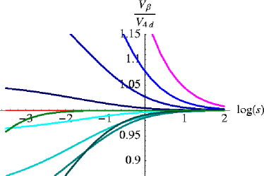
Figure 1: Ratio of the gravitational potential to the 4d one $V_{\beta}/V_{4d}$ as a function of $\log(s)=\log(r/L)$. The pink curve (top one) represents the pure RS case ($\beta=0$), and the blue curves (the ones below) are for $\beta=0.3,0.6,0.9$. The horizontal red curve represents the purely 4d case $\beta=1$, and the green curves below (from lightest to darkest) are for $\beta=1.1,1.5,2,100$. The curve with $\beta=100$ differs from the 4d only at very short distances $s\sim 10^{-3}$.

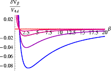
Figure 2: Relative departure of the gravitational potential to the 4d one $\left(V_{\beta}-V_{4d}\right)/V_{4d}$ as a function of the parameter $\beta$, for different values of $s$. The red horizontal curve is the purely 4d case and the curves below from red to blue (or from top to bottom) are evaluated at $s=0.25,0.5,1,2$.

As can be seen from Fig. 1, gravity can only be mildly weakened by the presence of GB terms with $\beta>1$, and in particular there is an upper bound on the modification of gravity, as is more clear in Fig. 2 where the ratio of the correction to the four-dimensional potential is represented as a function of $\beta$, for different distances $s$ to the point source.

Near the source, relative to the fundamental scale $L$, the integral in (34) goes as

$$\int_{0}^{\infty}\mathrm{d}x\rho_{\beta}(x)=-\frac{1-\beta}{2\beta},$$ (35)

for $\beta>0$, so that very close to the source, the gravitational potential is

$$V(r)\xrightarrow{r\rightarrow 0}-\frac{\kappa_{4}^{2}M}{2\pi r}\frac{1}{2\beta}.$$ (36)

Near the source, the gravitational potential therefore becomes four-dimensional again, but with a coefficient which is now changed. We recover the usual coefficient when $\beta=1$, and we see that as $\beta\rightarrow 0$, ie. in the RS limit, the coefficient diverges and the behaviour would be completely different from the case $\beta\neq 0$.

II.3 Implications for Cosmology

We now study the implications of a GB braneworld with $\beta\geq 1$ for cosmology. Previous works have studied the consequences of the GB term in cosmology Nojiri:2000gv ; Dufaux:2004qs ; Tsujikawa:2004dm , but most of these studies have focused on the regime where $\beta\ll 1$, as one would expect if this term arose from quantum/string corrections.

From the boundary condition (13) in the background, the modified Friedmann equation is:

$$H^{2}=\left\{\begin{array}[]{ll}\frac{1}{\ell^{2}\beta}\left[|1-\beta|\cosh\frac{2}{3}\chi-1\right]&\text{if}\ \beta\neq 1\\ \frac{1}{\ell^{2}}\left[\left(1+\frac{\rho}{\lambda}\right)^{2/3}-1\right]&\text{if}\ \beta=1,\end{array}\right.$$ (39)

with

$$\sinh\chi=\frac{\ell\kappa_{5}^{2}\lambda}{2}\sqrt{\frac{\beta}{2(1-\beta)^{3}}}\left(1+\frac{\rho}{\lambda}\right)\ \ \text{for }\beta<1$$ (40)

$$\cosh\chi=\frac{\ell\kappa_{5}^{2}\lambda}{2}\sqrt{\frac{\beta}{2(\beta-1)^{3}}}\left(1+\frac{\rho}{\lambda}\right)\ \ \text{for }\beta>1,$$ (41)

which generalizes the result in Dufaux:2004qs ; Tsujikawa:2004dm to more general cases of $\beta$.

II.3.1 Low-energy regime

At low energies compared with the brane tension, $\rho\ll\lambda$, the Friedmann equation (39) recovers a four-dimensional behavior: $H^{2}\simeq\frac{\kappa_{4}^{2}}{3}\rho$, and the higher-dimensional nature of the theory won’t affect the cosmological evolution within this range of energy. This approximation is valid as long as $\rho\ll\rho_{\lambda}$, where $\rho_{\lambda}=\frac{2(3-\beta)}{\ell\kappa_{5}^{2}}=2(3-\beta)(1+\beta)\left(L\kappa_{4}\right)^{-2}$. Assuming that $L=\left(1+\beta\right)\ell$ is of the order of $0.1$mm, the critical density is then of order $\rho_{\lambda}\simeq 2(3-\beta)(1+\beta)M^{4}_{\text{EW}}$, where $M_{\text{EW}}$ is the electroweak scale. For $\beta\sim 1$, this takes an order of magnitude of $\rho_{\lambda}\simeq 8M^{4}_{\text{EW}}$.

However one might be worried here that this low-energy effective theory is never a good approximation when the parameter $\beta$ is such that $\lambda=0$ (ie. when $\beta\simeq 3$). This is however never the case. Expanding the expression (39) for small $\rho$, we get

$$H^{2}=\frac{\kappa_{5}^{2}}{3}\rho+\frac{1}{36}\frac{1-3\beta}{\left(1+\beta\right)^{3}}L^{2}\kappa_{4}^{4}\rho^{2}+\mathcal{O}\left(L^{4}\kappa_{4}^{6}\rho^{3}\right),$$ (42)

so that the low-energy effective-theory is actually a good approximation as long as $\rho\ll\rho_{c}$, where $\rho_{c}=\frac{12\left(1+\beta\right)^{3}}{\left(3\beta-1\right)L^{2}\kappa_{4}^{2}}\sim\frac{12\left(1+\beta\right)^{3}}{\left(3\beta-1\right)}M^{4}_{\text{EW}}$. Such that when $\beta=1$, the real bound is $\rho_{c}\sim 48M^{4}_{\text{EW}}$ and when the brane tension vanishes, $\beta\simeq 3$, $\rho_{c}\sim 96M^{4}_{\text{EW}}$. The low-energy effective limit is therefore obtained even before what would be expected from the requirement that $\rho\ll\lambda$, if $\beta>1$.

In order to recover four-dimensional behavior right after inflation, we need the reheating temperature to be much smaller than this critical scale. Typical inflationary models occur at energies much larger than this scale, but there exist models which occur at energy scales of order of the electroweak scale, such as Ref. vanTent:2004rc . In this specific model, the reheating temperature is of order $T_{\text{Re}}\sim 0.43M_{\text{EW}}$, so the energy scale at the end of inflation is $\rho_{\text{Re}}\sim 0.03M^{4}_{\text{EW}}$. At the end of this inflationary model, the energy scale will be of order $\rho_{\text{Re}}\sim 7.10^{-4}\rho_{c}$, if $\beta\sim 1$. However, it might still be possible to imagine reheating mechanisms that could accomodate this modification of the standard Friedmann equation. The only real constraint is therefore that nucleosynthesis begins at energies below this critical scale. The energy scale at the beginning of nucleosynthesis is usually taken to be of order $\rho_{n}\sim 10^{-28}M^{4}_{\text{EW}}$, which is clearly much below the critical value.

The low-energy regime will therefore be a good approximation and the presence of the extra-dimension or the GB terms won’t affect cosmology at scales after inflation. We therefore argue that having large GB terms in the bulk is not incompatible with observations.

Furthermore, it has been shown that the presence of these GB terms might actually help to resurrect steep inflation driven by an exponential potential, as pointed out in Tsujikawa:2004dm , as well as quadratic and quartic potential inflationary models. The presence of $\rho^{2}$ terms in the Friedmann equation of the RS model, have raised the possibility of having a steep inflation scenario on the brane Maartens:1999hf . In the present case, we find at high energies

$$H^{2}\approx\frac{1}{\ell^{2}}\left(\frac{\ell\kappa_{5}^{2}}{4\beta}\rho\right)^{2/3}\ll\frac{\kappa_{5}^{2}}{4\beta\ell}\rho.$$ (43)

It is therefore less steep than normal inflation. The model of steep inflation will hence be invalid in this case.

II.3.2 Gravitational waves

To finish this section on cosmological consequences, we comment on the behaviour of gravitational waves during inflation. It has been shown in Ref. Dufaux:2004qs , that the presence of GB terms lead to a modified amplitude for the tensor perturbations. In particular, their amplitude is shown to first increase with energy scale, just as in the RS scenario, but as second stage, to decrease asymptotically. Using the same notation as in Dufaux:2004qs , the tensor amplitude is indeed shown to be of the form

$$A_{T}^{2} = \kappa_{4}^{2}\left(\frac{H^{2}}{2\pi}\right)^{2}F_{\beta}^{2}\left(\ell H\right)$$ (44)

$$F_{\beta}^{-2}(x) = \sqrt{1+x^{2}}-\left(\frac{1-\beta}{1+\beta}\right)x^{2}\sinh^{-1}\frac{1}{x}.$$ (45)

In the usual four-dimensional theory, the second term in the expression for $F_{\beta}^{-2}$ vanishes, and $F^{2}$ decreases monotonically as a function of the energy. In the RS case, however, $F_{0}^{2}$ increases monotonically. This behaviour is perturbed by the presence of GB terms, which usually follow the same behaviour as for RS at low-energy, before starting to decrease as in the four-dimensional case. The gravitational waves therefore increase above standard level before decreasing asymptotically as mentioned in Dufaux:2004qs . However, if the GB are important enough, in particular if $\beta>1$, they won’t have time to follow the RS behaviour before adopting the four-dimensional one, and the usual behaviour pointed out in Dufaux:2004qs will no longer be valid. The ratio of tensor to scalar perturbations amplitude will therefore remain close to the four-dimensional one within this regime.

II.4 Stability

When $-1<\beta<1$, no ghosts are present in the theory, see Ref. Cho:2001su . It has been shown in Deser:1987uk ; Maeda:2003vq , that in absence of any cosmological constant, EH-GB theories in more than four dimensions admit an AdS solution, beside the flat-Minkowski solution. This is indeed precisely the behaviour we get in (10) when $\beta=2$. Although this solution seems a priori well-defined and follows from a consistent theory of gravity, it has been shown in Ref. Deser:1989jm , that it corresponds to a gravitationally unstable solution. The ADM mass of any massive object living in the five-dimensional bulk will be negative which signals an instability Gleiser:2006yz ; Cai:2001dz , although interesting work in Ref. Gibbons:2004au has suggested that even a negative ADM mass object could be stable with suitable boundary conditions. Writing $\alpha=\beta\,\ell^{2}$, the equation relating the AdS length scale to the bulk cosmological constant is then quadratic in $\ell^{2}$: $\Lambda=-6/\ell^{2}+3\alpha/\ell^{4}$ such that there are two kind of solutions for $\ell^{2}$:

$$\ell^{2}=-\frac{3}{\Lambda}\left(1\pm\sqrt{1+\frac{\alpha\Lambda}{3}}\right),$$ (46)

the solution with the upper sign corresponds to the solution for which we recover the RS limit when $\alpha=0$. This represents the gravitationally stable branch. In order to recover the self-interacting AdS solution in absence of the cosmological constant, one should however consider the solution with the lower minus sign such that $\ell^{2}=\alpha/2$.

Any solution with $\beta>2$, ie. with $\Lambda>0$, must come from the solution with the lower sign, ie. the unstable solution. For $\Lambda<0$ (ie. for $\beta<2$), the maximum value $\alpha$ can take in any of the two branches is $\alpha<\alpha_{c}=-3/\Lambda$. This translates into a maximal value for the parameter $\beta$: $\beta<\beta_{c}=\left(1\pm\sqrt{1+\alpha\Lambda/3}\right)^{-1}$. Any solution with $\beta>1$ must therefore have originated from the branch with the lower sign (unless $\alpha<0$) which appears gravitationally unstable when positive matter is introduced in the bulk, as mentioned in Deser:1989jm . This can easily be understood from the Einstein equation (17). If some matter with stress-energy $\tau^{b}_{\mu\nu}$ was introduced in the bulk, the right hand side of the Einstein equation would be of the form $\left(1-\beta\right){}^{(5)\!}\Box h_{\mu\nu}=-2\kappa_{5}^{2}\tau^{b}_{\mu\nu}$. When $\beta>1$, matter will couple to gravity with the wrong sign, leading to naked singularities. When $\beta>1$, one should therefore consider matter to be introduced with the opposite sign in the bulk, for the theory to make sense gravitationally. We may note that the back-reaction from bulk gravitational waves won’t produce any instability, since they will enter with the correct sign in the modified Einstein equation.

In what follows, we take a slightly different approach, and present an alternative model where the bulk action remains the conventional EH one, with the conventional sign for gravity in the bulk. Instead, the price to pay will be to invert the contribution from the brane action. Despite this, conventional gravity is recovered on the brane at low energies.

III Alternative approach

III.1 EH-RS model

We consider in what follows the alternative approach, where the bulk gravitational action is the same as in the RS model, but the boundary action is unconventional:

$$S^{(\text{5d})} = \frac{1}{2\kappa_{5}^{2}}\int\mathrm{d}^{5}x\sqrt{-g}\Bigl{[}\mathrm{R}-2{\Lambda}\Bigr{]}-S^{(\text{4d})}_{b}$$ (47)

$$S^{(\text{4d})}_{b} = \int_{\text{brane}}\mathrm{d}^{4}x\sqrt{-q}\left[\frac{\tilde{\beta}}{2\tilde{\kappa}^{2}}R+\mathcal{L}_{m}+{\tilde{\lambda}}-2K\right],$$

where we take $\tilde{\kappa}^{2}=\kappa_{5}^{2}/\ell$, and we consider $\tilde{\beta}>0$. We consider the brane tension to be fine-tuned to the canonical value ${\tilde{\lambda}}=6/\kappa_{5}^{2}\ell$. This can be seen as a combination of the RS model and the Dvali-Gabadadze-Porrati (DGP) one Dvali:2000rv (although we do not concentrate on the self-accelerating branch of the DGP model), with the “wrong” sign for the brane action. For a realization of this model from string theory, see Ref. Antoniadis:2002tr .

We can analyze this model in the same manner as the RS model by replacing the usual four-dimensional stress-energy tensor for matter field by:

$$T^{\text{RS}}_{\mu\nu}\rightarrow-T_{\mu\nu}+\frac{\tilde{\beta}}{\tilde{\kappa}^{2}}G_{\mu\nu},$$ (48)

where now $T_{\mu\nu}$ is the stress-energy of matter field on the brane: $T_{\mu\nu}=-\frac{2}{\sqrt{-q}}\frac{\delta}{\delta q^{\mu\nu}}\sqrt{-q}\mathcal{L}_{m}$.

The low-energy effective theory in the RS model is $G_{\mu\nu}=\tilde{\kappa}^{2}T^{\text{RS}}_{\mu\nu}$, and therefore gets replaced by

$$G_{\mu\nu}=\frac{\tilde{\kappa}^{2}}{\tilde{\beta}-1}T_{\mu\nu}$$ (49)

in the new theory (47). The parameter $\tilde{\beta}$ should therefore satisfy $\tilde{\beta}>1$, for matter to couple to gravity the right way. In the IR regime, this theory will therefore be completely consistent.

Considering a homogeneous and isotropic background, the Israël matching condition in the RS case is $\rho^{\text{RS}}={\tilde{\lambda}}\left(\sqrt{1+\ell^{2}H^{2}}-1\right)$. Using the transformation $\rho^{\text{RS}}\rightarrow-\rho+{\tilde{\lambda}}\ell^{2}H^{2}/2$, this equation becomes quadratic for $H^{2}$, and as pointed out in the DGP model, there are therefore two branches for the solution:

$$H^{2}=\frac{2(\tilde{\beta}-1)}{\tilde{\beta}^{2}\ell^{2}}\left[-1+\frac{\tilde{\beta}}{\tilde{\beta}-1}\frac{\rho}{{\tilde{\lambda}}}\pm\sqrt{1+2\frac{\tilde{\beta}}{(\tilde{\beta}-1)^{2}}\frac{\rho}{{\tilde{\lambda}}}}\right].$$ (50)

The branch with the upper sign is the one that recovers the usual four-dimensional Friedmann equation at low-energy, $\rho\ll{\tilde{\lambda}}$. The other solution, presents a self-accelerating behaviour at low-energy $\ell^{2}H^{2}\simeq 4(1-\tilde{\beta})/\tilde{\beta}^{2}$, and has been pointed out in Dvali:2000rv , as a potential explanation for the cosmological constant problem (note that this solution could only be possible here if $\tilde{\beta}<1$, which is not the case we consider here). Recent arguments confirm the instability of this branch, see Ref. Koyama:2005tx ; Charmousis:2006pn for recent reviews on the subject.

III.2 Linearized Gravity

In what follows, we concentrate on the solution (50) with the upper sign, and study linearized gravity around the five-dimensional AdS, with $\rho=0$. We follow the same procedure as in section II.2, using the same notation. We study the perturbations generated by the presence of some matter source $T_{\mu\nu}$ on the brane. In the RS model, the presence of this source generates the induced perturbations on the brane:

$$\bar{h}_{\mu\nu}^{\text{RS}} = \frac{\kappa_{5}^{2}}{\sqrt{-\Box}}\frac{K_{2}\left(\sqrt{-\Box}\ell\right)}{K_{1}\left(\sqrt{-\Box}\ell\right)}\left(T_{\mu\nu}^{\text{RS}}-\frac{1}{3}T^{\text{RS}}\eta_{\mu\nu}+\frac{1}{3\Box}T^{\text{RS}}_{,\mu\nu}\right)$$ (51)

$$-\frac{\tilde{\kappa}^{2}}{3\Box}\left(T^{\text{RS}}\eta_{\mu\nu}+\frac{2}{\Box}T^{\text{RS}}_{,\mu\nu}\right),$$

in de Donder gauge Garriga:1999yh ; deRham:2004yt . Using this result, and performing the transformation

$$T^{\text{RS}}_{\mu\nu} \rightarrow -T_{\mu\nu}+\frac{\tilde{\beta}}{\tilde{\kappa}^{2}}\left(R_{\mu\nu}-\frac{1}{2}R\eta_{\mu\nu}\right)$$ (52)

$$= -T_{\mu\nu}+\frac{\tilde{\beta}}{2(\tilde{\beta}-1)}T\eta_{\mu\nu}-\frac{\tilde{\beta}}{2\tilde{\kappa}^{2}}\Box\bar{h}_{\mu\nu},$$

we obtained the induced perturbations on the brane

$$\bar{h}_{\mu\nu}=-\frac{2\tilde{\kappa}^{2}}{(\tilde{\beta}-1)}\Biggl{[}\frac{1}{\Box}\left(T_{\mu\nu}-\frac{1}{2}T\,\eta_{\mu\nu}\right)+\frac{\ell\hat{K}_{\tilde{\beta}}}{\sqrt{-\Box}}\Sigma_{\mu\nu}\Biggr{]}$$ (53)

where

$$\hat{K}_{\tilde{\beta}}=\frac{K_{0}\left(\sqrt{-\Box}\ell\right)}{2(\tilde{\beta}-1)K_{1}\left(\sqrt{-\Box}\ell\right)+\tilde{\beta}\sqrt{-\Box}\ell K_{0}\left(\sqrt{-\Box}\ell\right)},$$ (54)

and $\Sigma_{\mu\nu}$ as defined in (23).

At low energies, we therefore recover the four-dimensional behaviour as expected, with $\kappa_{4}^{2}=\tilde{\kappa}^{2}/(\tilde{\beta}-1)$. This theory only makes sense if $\tilde{\beta}>1$, in which case the KK corrections in (53), come with a negative sign, similarly as in (26), giving rise to a weaker gravity at small scales.

This theory will therefore behave similarly at small scales as the GB-RS theory described previously, in the regime where $\tilde{\beta}>1$. Far away from the brane, this theory will however appear well-defined, and will not present the instabilities pointed out before.

III.3 Brane energy conditions

In this section we demonstrate that the brane satisfies, in certain limits, the usual energy conditions. We define the total energy of the brane to be the sum of the canonical brane tension ${\tilde{\lambda}}$ and contributions from the EH term and brane matter:

$$T^{\text{tot}}_{\mu\nu} = \frac{2}{\sqrt{-q}}\frac{\delta\sqrt{-q}}{\delta q^{\mu\nu}}\left(\frac{\tilde{\beta}}{2\tilde{\kappa}^{2}}R+\mathcal{L}_{m}+{\tilde{\lambda}}\right)$$ (55)

$$= \frac{\tilde{\beta}}{\tilde{\kappa}^{2}}G_{\mu\nu}-T_{\mu\nu}-{\tilde{\lambda}}\,q_{\mu\nu}.$$ (56)

First of all, at low energies the total brane stress energy is equal to the brane tension plus a term proportional to the stress energy of matter. Using the relation (49), valid at low energies, we have

$$T^{\text{tot}}_{\mu\nu}=-{\tilde{\lambda}}\,q_{\mu\nu}+\frac{1}{\tilde{\beta}-1}T_{\mu\nu}.$$ (57)

If the brane matter $T_{\mu\nu}$ satisfied either the weak or null energy conditions, then it is immediately clear that $T^{\text{tot}}_{\mu\nu}$ satisfies the same conditions. We can also see what happens at high energies, but at long wavelengths using the separate universes approach Guth:1982ec ; Starobinsky:1986fx whereby long wavelength perturbations are modeled locally as a FRW universe with curvature. Then the null energy condition amounts to $p+\rho\geq 0$ and the weak energy condition has the additional constraint $\rho\geq 0$. Using the effective Friedmann equation for the brane (50) we can infer the total energy density on the brane

$$\rho_{\text{tot}} = \frac{3\tilde{\beta}}{\tilde{\kappa}^{2}}H^{2}-\rho+{\tilde{\lambda}}$$ (58)

$$= \frac{{\tilde{\lambda}}}{\tilde{\beta}}+{\tilde{\lambda}}\frac{(\tilde{\beta}-1)}{\tilde{\beta}}\sqrt{1+2\frac{\tilde{\beta}}{(\tilde{\beta}-1)^{2}}\frac{\rho}{{\tilde{\lambda}}}}\ .$$

It is clear that $\rho_{\text{tot}}$ satisfies $\rho_{\text{tot}}\geq{\tilde{\lambda}}/{\tilde{\beta}}$ and so provided $\rho$ satisfies the null energy condition then $\rho_{\text{tot}}$ satisfies the weak and null energy conditions.

We can extend this argument by considering the effect of taking the bulk to be Schwarzschild-AdS with either a positive or negative ADM mass. In this case we recover a similar result as long as the brane is sufficiently far away from the bulk black hole (ie. outside the Schwarzschild radius of this object if its ADM mass is positive).

III.4 Implications for Cosmology

As mentioned previously, provided we consider the stable branch of the solution (50), the usual four-dimensional Friedmann equation is recovered at low-energy $H^{2}=\kappa_{4}^{2}/3\,\rho$, when $\rho\ll 2(1-\tilde{\beta})^{2}{\tilde{\lambda}}$, where the four-dimensional gravitational coupling constant is as defined previously $\kappa_{4}^{2}=\tilde{\kappa}^{2}/(\tilde{\beta}-1)$. This low-energy will therefore be satisfied as long as $\rho\ll 12(\tilde{\beta}-1)\left(\ell\kappa_{4}\right)^{-2}$, so that if $(\tilde{\beta}-1)\sim 1$, this constraint will be satisfied for $\rho\ll 12M_{\text{EW}}^{4}$. Similarly as in section II.3.1, this low-energy regime, will be consistent with scenarios of inflation with a very small reheating temperature, such as the one proposed in Ref. vanTent:2004rc . However, this model also recovers a four-dimensional behaviour at high-energy $H^{2}\simeq 2\tilde{\kappa}^{2}/{\tilde{\beta}}\,\rho$, when $\rho\gg{\tilde{\lambda}}\sim M_{\text{EW}}^{4}$. Within this limit, cosmology will not be perturbed, and the expression for the slow-roll parameters will remain very similar to the usual four-dimensional ones

$$\epsilon=-\frac{\dot{H}}{H^{2}}\simeq\frac{\tilde{\beta}}{2\tilde{\kappa}^{2}}\frac{V^{\prime}{}^{2}}{V^{2}},\hskip 20.0pt\eta=\frac{V^{\prime\prime}}{3H^{2}}\simeq\frac{\tilde{\beta}}{\tilde{\kappa}^{2}}\frac{V^{\prime\prime}}{V}.$$ (59)

In the limit $\tilde{\beta}\rightarrow 0$, the relations are no longer valid since the Friedmann equation becomes linear at high-energy $H^{2}\sim\rho^{2}/{\tilde{\lambda}}^{2}$ in the pure RS model. We therefore have a similar conclusion that the scenario of steep inflation as is usually possible in the pure RS model will no longer give a consistent scenario for inflation in this model.

IV Stability of compact stars

The astrophysical implications of the modification of gravity at small scales in typical braneworld models have been studied in particular in Germani:2001du ; Wiseman:2001xt . Although the vacuum solution around a massive object confined in four-dimensions is no longer the Schwarzschild metric Germani:2001du , neutron stars do not seem to be affected by the higher order corrections in the brane according to the numerical studies of Wiseman:2001xt . In what follows, we give some brief comments on how the stability of white dwarf and neutron stars can be improved by the presence of GB terms in the bulk, or in the alternative scenario presented in the previous section.

Following the many-body analysis of Ref. Azam:2005dw , when gravity on the brane is modified, the Chandrasekhar ground state (see Ref. Chandrasekhar:1984 ) does not seem to be affected by the RS corrections. However, a more precise analysis performed very recently, shows the existence of another unbounded minimum of the energy functional at very small radius, when RS corrections are present Azam:2006pk . The existence of this unbounded minimum makes the Chandrasekhar minimum metastable, although the tunneling probability to the new ground state is exponentially suppressed (see Ref. Azam:2006pk for details of the argument and the computation), and it is not clear whether the argument makes sense within the Schwazschild radius of the star.

In what follows, we review the argument when the KK modes bring a negative correction to the zero mode and gravity becomes weaker at short distances. For that we follow closely the analysis of Azam:2006pk and use the same notation. In particular $M_{0}$ and $R_{0}$ are the typical mass and radius of helium white dwarfs. We consider a star with mass $M=\bar{M}M_{0}$ and radius $r=\bar{r}R_{0}$. We write $x_{F}=\bar{M}^{1/3}/\bar{r}$.

In the pure RS scenario, the first order correction to the gravitational potential, leads to a short range correction of the energy functional $\Xi_{c}$, going like $\ell^{2}/r^{3}$. We write this correction $\gamma_{0}x_{F}^{3}$, with $\gamma_{0}\sim\ell^{2}/R_{0}^{2}$, the exact coefficient in the expression of $\gamma_{0}$ depends on the star parameters, but is of order $1$, and is always positive in the RS model, since the KK corrections give positive correction to the zero mode and make gravity stronger at short-distances. The modified energy functional is then of the form

$$\Xi_{c}=\frac{3\pi^{2}\bar{\mathcal{E}}(x_{F})}{x_{F}^{3}}-1-\bar{M}^{2/3}x_{f}-\gamma_{0}x_{F}^{3},$$ (60)

where the two first terms are related to the kinetic energy of the free Fermi electron gas, and the function $\bar{\mathcal{E}}(x_{F})$ is such that, for very small radius, $x_{F}>>1$, $\frac{3\pi^{2}\bar{\mathcal{E}}(x_{F})}{x_{F}^{3}}\rightarrow\frac{3}{4}x_{F}$. The third term represents the contribution from the Newton gravitational potential and the last term the leading correction from the KK modes in the RS scenario.

Below some critical mass, this energy functional has a unique minimum which is the Chandrasekhar ground state, if the mass $\bar{M}$ is below some critical value. However, for very small radius, the energy functional is

$$\Xi_{c}\xrightarrow{x_{F}\gg 1}\left(\frac{3}{4}-\bar{M}^{2/3}\right)x_{F}-1-\gamma_{0}x_{F}^{3},$$ (61)

such that in presence of RS corrections, ($\gamma_{0}>0$), the functional goes to infinite negative values as the radius goes to zero, the Chandrasekhar vacuum is then no longer the ground state, and is metastable. This is a simple consequence of the fact that gravity becomes stronger at short distances in that model, and the kinetic energy is no longer able to compensate the increased gravitational potential. However the situation is different if gravity is weaker at short distances, and as one would expect, the stability of the star is then increased in such a situation.

We now examine the same situation when GB terms are included in the bulk (the situation in the alternative scenario III, is completely analogous). In both scenarios, when $\beta>1$ (or $\tilde{\beta}>1$), gravity is indeed weaker at short distances and we don’t expect the previous situation to occur. The sign of the leading correction to the gravitational potential is indeed negative as we have shown in (31). The leading correction in (60), will therefore have the opposite sign since the corrections will now be modified to: $\gamma_{\beta}\,x_{F}^{3}=\left(1-\beta\right)/\left(1+\beta\right)\gamma_{0}x_{F}^{3}\sim\left(1-\beta\right)/\left(1+\beta\right)\ell^{2}/r^{3}$, such that when $\beta>1$, $\gamma_{\beta}$ is now negative. In that case, the argument presented above will no longer be valid. To be more precise, we explore the same situation in the limit $x_{F}\gg 1$ when GB terms are present. As pointed out in (36), the modification to the gravitational potential will recover a $r^{-1}$ behaviour, such that the corrections will now be of the form $\gamma_{\beta}x_{F}$. The energy functional will therefore be

$$\Xi_{c}\xrightarrow{x_{F}\gg 1}\left(\frac{3}{4}+\frac{\beta-1}{\beta+1}\gamma_{0}-\bar{M}^{2/3}\right)x_{F}-1.$$ (62)

When the contribution from the GB terms is below a critical value $\beta<\beta_{c}<1$, where $\beta_{c}$ is such that the term in bracket in (62) vanishes, the situation is similar to the one pointed out in Azam:2006pk , and the Chandrasekhar vacuum is therefore metastable. However, when $\beta$ is important, $\beta>\beta_{c}>1$, there is no longer any unbounded minimum and the Chandrasekhar vacuum remains the ground state of the theory. The presence of important GB terms can therefore help recovering a four-dimensional behaviour which can be broken in a pure RS scenario. The same argument will be valid when the alternative approach of section III is instead considered.

V Summary

The observation of weaker gravity at short scales could present a real challenge to theoretical physics. Having a gravitational potential which falls off slower than $1/r$ is usually hard to obtain without the presence of ghosts in the theory, or considering the exchange of massive spin-1 bosons which are highly constrained by experiments on the Equivalence Principle. Braneworld models usually lead to a gravitational potential which is stronger at short distances, due to the additional contribution from the KK modes. In this work we presented two possible models where the KK modes contribute with an opposite sign to the usual four-dimensional potential, leading to weaker gravity at short distances. This comes at the price of introducing instabilities in the theory which may no longer be quantized the same way as ordinary four-dimensional gravity at high-energy. However, at low-energy on the brane, we recover a four-dimensional behaviour and the theory remains well-defined in that regime. As a test of the proposed models, we studied the implications for cosmology and showed that no distinctions from four-dimensional cosmology will be observed after the beginning of nucleosynthesis. Within these models, the stability of white dwarfs and neutron stars against gravitational collapse is typically improved since the gravitational potential is weaker near the center of the star.

Appendix A Contribution from the KK modes

Using the result from (26), the contribution of the KK modes to the gravitational potential is

$$V_{KK}=\frac{1-\beta}{1+\beta}\int\mathrm{d}k\frac{k\sin kr}{2\pi^{2}r}\frac{K_{0}\left(k\ell\right)}{k\left((1+\beta)K_{1}\left(k\ell\right)+\beta k\ell K_{0}\left(k\ell\right)\right)}.$$ (63)

We can either evaluate this integral numerically using some regularization scheme, or use the following property

$$\frac{1}{k}\frac{\left(1-\beta\right)^{2}}{\left(1+\beta\right)}\frac{K_{0}(kl)}{(1+\beta)K_{1}(kl)+kl\beta K_{0}(kl)}=\int_{0}^{\infty}\mathrm{d}m\frac{4}{\pi^{2}ml\left(m^{2}+k^{2}\right)}\frac{1}{\tilde{J}_{\beta}(ml)^{2}+\tilde{Y}_{\beta}(ml)^{2}},$$ (64)

where $Y_{n}$ and $J_{\alpha}$ are the Bessel functions and we use the notation:

$$\tilde{Z}_{\beta}(x)=Z_{1}(x)+\frac{\beta}{1-\beta}\,xZ_{2}(x).$$ (65)

Using this relation, we therefore have:

$$V_{KK} = \frac{1}{2\pi^{2}r(1-\beta)}\int\mathrm{d}m\ \frac{4}{\pi^{2}ml}\frac{1}{\tilde{J}_{\beta}(ml)^{2}+\tilde{Y}_{\beta}(ml)^{2}}\int\mathrm{d}k\frac{k\sin kr}{m^{2}+k^{2}}$$ (66)

$$= \frac{1}{4\pi r(1-\beta)}\int\mathrm{d}m\ e^{-mr}\frac{4}{\pi^{2}ml}\frac{1}{\tilde{J}_{\beta}(ml)^{2}+\tilde{Y}_{\beta}(ml)^{2}}$$

$$\simeq \frac{1}{4\pi r(1-\beta)}\int\mathrm{d}m\ e^{-mr}ml\left(\frac{1-\beta}{1+\beta}\right)^{2}\left[1-m^{2}\ell^{2}\left(\frac{1}{2}-\frac{1-\beta}{1+\beta}\left(\gamma-\log\frac{2}{m\ell}\right)\right)+\cdots\right]$$

$$\simeq \frac{1}{4\pi r}\frac{1-\beta}{\left(1+\beta\right)^{2}}\left[\frac{\ell}{r^{2}}+\frac{2\ell^{3}}{r^{4}}\left(\frac{4-7\beta}{1+\beta}-3\frac{1-\beta}{1+\beta}\log\frac{2r}{l}\right)\cdots\right].$$

References

- (1) C. D. Hoyle, U. Schmidt, B. R. Heckel, E. G. Adelberger, J. H. Gundlach, D. J. Kapner and H. E. Swanson, Phys. Rev. Lett. 86 (2001) 1418 [arXiv:hep-ph/0011014]; E. G. Adelberger [EOT-WASH Group], arXiv:hep-ex/0202008; C. D. Hoyle, D. J. Kapner, B. R. Heckel, E. G. Adelberger, J. H. Gundlach, U. Schmidt and H. E. Swanson, Phys. Rev. D 70, 042004 (2004) [arXiv:hep-ph/0405262]; E. G. Adelberger, Prepared for 3rd Meeting on CPT and Lorentz Symmetry (CPT 04), Bloomington, Indiana, 4-7 Aug 2004
- (2) E. G. Adelberger, B. R. Heckel and A. E. Nelson, Ann. Rev. Nucl. Part. Sci. 53, 77 (2003) [arXiv:hep-ph/0307284].
- (3) N. Arkani-Hamed, S. Dimopoulos and G. R. Dvali, Phys. Lett. B 429, 263 (1998) [arXiv:hep-ph/9803315]; I. Antoniadis, N. Arkani-Hamed, S. Dimopoulos and G. R. Dvali, ibid. 436, 257 (1998) [arXiv:hep-ph/9804398].
- (4) L. Randall and R. Sundrum, Phys. Rev. Lett. 83, 4690 (1999) [arXiv:hep-th/9906064].
- (5) J. Garriga and T. Tanaka, Phys. Rev. Lett. 84, 2778 (2000) [arXiv:hep-th/9911055].
- (6) P. Callin and F. Ravndal, Phys. Rev. D 70, 104009 (2004) [arXiv:hep-ph/0403302]; P. Callin, arXiv:hep-ph/0407054.
- (7) P. Callin and C. P. Burgess, arXiv:hep-ph/0511216.
- (8) R. Sundrum, Phys. Rev. D 69, 044014 (2004) [arXiv:hep-th/0306106].
- (9) R. Sundrum, Nucl. Phys. B 690, 302 (2004) [arXiv:hep-th/0310251].
- (10) T. Biswas, A. Mazumdar and W. Siegel, arXiv:hep-th/0508194.
- (11) G. L. Smith, C. D. Hoyle, J. H. Gundlach, E. G. Adelberger, B. R. Heckel and H. E. Swanson, Phys. Rev. D 61, 022001 (2000).
- (12) J. M. Cline, S. Jeon and G. D. Moore, Phys. Rev. D 70, 043543 (2004) [arXiv:hep-ph/0311312].
- (13) S. W. Hawking and T. Hertog, Phys. Rev. D 65, 103515 (2002) [arXiv:hep-th/0107088].
- (14) J. T. Wheeler, Nucl. Phys. B 273, 732 (1986).
- (15) I. P. Neupane, Phys. Lett. B 512, 137 (2001) [arXiv:hep-th/0104226].
- (16) N. Deruelle and M. Sasaki, Prog. Theor. Phys. 110, 441 (2003) [arXiv:gr-qc/0306032].
- (17) K. i. Maeda and T. Torii, Phys. Rev. D 69, 024002 (2004) [arXiv:hep-th/0309152].
- (18) I. P. Neupane, Class. Quant. Grav. 19, 5507 (2002) [arXiv:hep-th/0106100].
- (19) Y. M. Cho and I. P. Neupane, Int. J. Mod. Phys. A 18, 2703 (2003) [arXiv:hep-th/0112227].
- (20) K. A. Bronnikov, S. A. Kononogov and V. N. Melnikov, arXiv:gr-qc/0601114.
- (21) D. G. Boulware and S. Deser, Phys. Rev. Lett. 55, 2656 (1985).
- (22) K. A. Meissner and M. Olechowski, Phys. Rev. Lett. 86, 3708 (2001) [arXiv:hep-th/0009122], K. A. Meissner and M. Olechowski, Phys. Rev. D 65, 064017 (2002) [arXiv:hep-th/0106203].
- (23) N. Deruelle and J. Madore, arXiv:gr-qc/0305004.
- (24) Z. Kakushadze, JHEP 0110, 031 (2001) [arXiv:hep-th/0109054].
- (25) G. W. Gibbons and S. W. Hawking, Phys. Rev. D 15, 2752 (1977).
- (26) R. C. Myers, Phys. Rev. D 36, 392 (1987).
- (27) S. Deser, Class. Quant. Grav. 4, L99 (1987).
- (28) S. Deser and Z. Yang, Class. Quant. Grav. 6, L83 (1989).
- (29) J. Crisostomo, R. Troncoso and J. Zanelli, Phys. Rev. D 62, 084013 (2000) [arXiv:hep-th/0003271].
- (30) O. Corradini, Mod. Phys. Lett. A 20, 2775 (2005) [arXiv:hep-th/0405038].
- (31) W. Israel, Nuovo Cim. B 44S10, 1 (1966) [Erratum-ibid. B 48 (1967 NUCIA,B44,1.1966) 463].
- (32) S. C. Davis, Phys. Rev. D 67, 024030 (2003) [arXiv:hep-th/0208205]; E. Gravanis and S. Willison, Phys. Lett. B 562, 118 (2003) [arXiv:hep-th/0209076].
- (33) S. Nojiri and S. D. Odintsov, JHEP 0007, 049 (2000) [arXiv:hep-th/0006232]; M. Cvetic, S. Nojiri and S. D. Odintsov, Nucl. Phys. B 628, 295 (2002) [arXiv:hep-th/0112045]; S. Nojiri, S. D. Odintsov and S. Ogushi, Int. J. Mod. Phys. A 17, 4809 (2002) [arXiv:hep-th/0205187].
- (34) J. F. Dufaux, J. E. Lidsey, R. Maartens and M. Sami, Phys. Rev. D 70, 083525 (2004) [arXiv:hep-th/0404161].
- (35) S. Tsujikawa, M. Sami and R. Maartens, Phys. Rev. D 70, 063525 (2004) [arXiv:astro-ph/0406078].
- (36) B. van Tent, J. Smit and A. Tranberg, JCAP 0407, 003 (2004) [arXiv:hep-ph/0404128].
- (37) R. Maartens, D. Wands, B. A. Bassett and I. Heard, Phys. Rev. D 62, 041301 (2000) [arXiv:hep-ph/9912464]; E. J. Copeland, A. R. Liddle and J. E. Lidsey, Phys. Rev. D 64, 023509 (2001) [arXiv:astro-ph/0006421]; M. Sami, N. Dadhich and T. Shiromizu, Phys. Lett. B 568, 118 (2003) [arXiv:hep-th/0304187].
- (38) Y. M. Cho, I. P. Neupane and P. S. Wesson, Nucl. Phys. B 621, 388 (2002) [arXiv:hep-th/0104227].
- (39) R. J. Gleiser and G. Dotti, arXiv:gr-qc/0604021.
- (40) R. G. Cai, Phys. Rev. D 65, 084014 (2002) [arXiv:hep-th/0109133].
- (41) G. W. Gibbons, S. A. Hartnoll and A. Ishibashi, Prog. Theor. Phys. 113, 963 (2005) [arXiv:hep-th/0409307].
- (42) G. R. Dvali, G. Gabadadze and M. Porrati, Phys. Lett. B 484, 112 (2000) [arXiv:hep-th/0002190]; G. R. Dvali, G. Gabadadze and M. Porrati, Phys. Lett. B 485, 208 (2000) [arXiv:hep-th/0005016]; G. R. Dvali and G. Gabadadze, Phys. Rev. D 63, 065007 (2001) [arXiv:hep-th/0008054]; C. Deffayet, G. R. Dvali and G. Gabadadze, Phys. Rev. D 65, 044023 (2002) [arXiv:astro-ph/0105068].
- (43) I. Antoniadis, R. Minasian and P. Vanhove, Nucl. Phys. B 648, 69 (2003) [arXiv:hep-th/0209030].
- (44) K. Koyama, Phys. Rev. D 72, 123511 (2005) [arXiv:hep-th/0503191].
- (45) C. Charmousis, R. Gregory, N. Kaloper and A. Padilla, arXiv:hep-th/0604086.
- (46) C. de Rham, Phys. Rev. D 71, 024015 (2005) [arXiv:hep-th/0411021].
- (47) A. H. Guth and S. Y. Pi, Phys. Rev. Lett. 49, 1110 (1982); S. W. Hawking, Phys. Lett. B 115, 295 (1982); A. A. Starobinsky, Phys. Lett. B 117 (1982) 175.
- (48) A. A. Starobinsky, JETP Lett. 42, 152 (1985) [Pisma Zh. Eksp. Teor. Fiz. 42, 124 (1985)]; D. S. Salopek, Phys. Rev. D 52, 5563 (1995) [arXiv:astro-ph/9506146].
- (49) C. Germani and R. Maartens, Phys. Rev. D 64, 124010 (2001) [arXiv:hep-th/0107011].
- (50) T. Wiseman, Phys. Rev. D 65, 124007 (2002) [arXiv:hep-th/0111057].
- (51) M. Azam and M. Sami, Phys. Rev. D 72, 024024 (2005) [arXiv:gr-qc/0502026].
- (52) S. Chandrasekhar, Rev. Mod. Phys. 56, 137 (1984); E. H. Lieb and H. T. Yau, Commun. Math. Phys. 112, 147 (1987).
- (53) M. Azam and M. Sami, arXiv:astro-ph/0603525.