On the Pionner Anomaly

Abstract

In this paper an explanation of the Pioneer anomaly is given, using the hypothesis of the time dependent gravitational potential. The implications of this hypothesis on the planetary orbits and orbital periods are given in section 2. In sections 3 and 4 we give a detailed explanation of the Pioneer anomaly, which corresponds to the observed phenomena.

1 Introduction

In 1998 an interesting paper by Anderson et al. (1998) was published, with indication that there is an unexplained frequency shift in the navigation of the spacecraft Pioneer 10 and 11. Namely, the detailed analysis of the frequencies of the round-trip signals from the spacecraft Pioneer 10 and Pioneer 11, yield to a slight disagreement with the expected frequencies. This small shift of the frequencies accumulates in time. Later a very detailed analysis of this phenomena was given by Anderson et al.(2002). Firstly, we give a short history about this effect, following the references (Anderson et al. 1998, 2002; Turyshev et al. 2004, 2005, 2006).

The spacecraft Pioneer 10 was launched on 1972 March 2, while Pioneer 11 was launched on 1973 April 5, and their aim was to explore the outer Solar System (Turyshev et al. 2006). They are the first spacecrafts that left the Solar System. The mentioned phenomena was detected in 1980 for the spacecraft Pioneer 10 for the first time, when it was about 20 AU far from the Sun, and the influence of the neighboring planets was negligible on the detected shift frequency. This phenomena was well examined for Pioneer 10 on the heliocentric distances 20-70 AU. Similar results were also obtained for the spacecraft Pioneer 11, but, unfortunately, after 1995 November the contact with Pioneer 11 was lost, and the research with Pioneer 11 was stopped. The last signal from Pioneer 10 was obtained in April 2002, when it was about 80 AU from the Sun.

The unexplained blue shift of the frequency is denoted by $a_{P}$ and it is introduced by the formula (15) in (Anderson et al. 2002), i.e.

$$[\nu_{obs}(t)-\nu_{model}(t)]_{DSN}=-\nu_{0}\frac{2a_{P}t}{c},\qquad\nu_{model}=\nu_{0}\Bigl{[}1-2\frac{v_{model}(t)}{c}\Bigr{]},$$

where $\nu_{0}$ is the reference frequency, the factor 2 is because of the two way data, $v_{model}$ is the modeled velocity of the spacecraft due to the gravitational and other forces and $\nu_{obs}$ is frequency of the re-transmitted signal observed by DSN antennae. Since $a_{P}$ is in the same units as the acceleration, it is also called anomaly acceleration and it is interpreted as if there is an acceleration toward the Sun of magnitude $a_{P}\approx(8.74\pm 1.33)\times 10^{-8}$cm s^-2. The existence of such an acceleration is almost impossible, because it would change the planetary orbits, while the astronomical observations do not show such change (Iorio 2006). So it would be more convenient to say ”Pioneer anomaly” than ”anomaly acceleration”. It is mentioned in (Anderson et al. 1998, 2002) that without using the acceleration $a_{P}$, the anomalous frequency shift can be interpreted as a ”clock acceleration” $-a_{t}=-2.8\times 10^{-18}$s s^-2.

There are several attempts to explore the possible sources of the Pioneer anomaly. The original efforts, including classical explanations (effects from sources external to the spacecraft, study of the on-board systematics and computational systematics) of this anomaly are not strong enough to explain the observed Doppler shift (Turyshev et al. 2006). So, the question of a possible new physics arises. There are several attempts to explore the possible sources of the Pioneer anomaly via non-classical Newtonian mechanics and general relativity. The ideas are quite different and here we mention some of them: Newtonian gravity as a long wavelength excitation of a scalar condensate inducing electroweak symmetry breaking (Consoli & Siringo 1999), time dependence of the gravitational constant $G$ (Sidharth 2000), higher order (or Yukawa-like) corrections to the Newtonian potential (Anderson et al. 1998), a scalar-tensor extension to the standard gravitational model (Clachi Novati et al. 2000), interaction of the spacecraft with a long-range scalar field coupled to gravity (Mbelek & Lachièze-Rey 1999; Cadoni 2004), a length or momentum scale-dependent cosmological term in the gravitational action functional (Modanese 1999), a local solar system curvature for light-like geodesics arising from the cosmological expansion (Rosales & Sánchez-Gomez 1999), influence of the cosmological constant at the scale of the Solar System (Nottale 2003), a 5-dimensional cosmological model with a variable extra dimensional scale-factor and static external space (Belayev 2001), a superstrong interaction of photons or massive bodies with the graviton background yielding a constant acceleration proportional to the Hubble constant (Ivanov 2001), using an expanded PPN formalism (Ostvang 2002), explanation using the Brans-Dicke theory of gravity (Capozzielo et al. 2001), explanation using braneworld theories (Bertolami & Páramos 2004), and so on (Foot & Volkas 2001; Guruprasad 1999, 2000; Wood & Moreau 2001; Crawford 1999; Ingersoll et al. 1999; Milgrom 2001; Munyaneza & Viollier 1999; Rañada 2005).

In this paper, we give new arguments and we upgrade the papers (Trenčevski 2005a, 2006) concerning the hypothesis the time dependent gravitational potential. In section 2 we give some results about the time dependent gravitational potential and in section 3 we will return to the Pioneer anomaly. The mathematical calculations will be shortened, while the physical interpretation will be emphasized.

2 Time dependent gravitational potential

In the recent paper (Trenčevski 2005a) and also in (Trenčevski 2006), an idea about linear change of the gravitational potential in the universe was developed. This linear (or almost linear) change is probably a consequence of the change of the density of the dark matter in the universe, but we shall consider only the consequence of this phenomena, not its origin. It can be interpreted in this way: the whole universe is inside of a shielded laboratory which falls freely in a gravitational field. Then, for a small time interval, the change of the gravitational potential can be considered to be almost linear. For simpler interpretation of the induced effects, we shall consider two observers: observer A in the shielded laboratory, where the gravitational potential changes linearly, and observer B outside the shielded laboratory, far from the gravitational field, where the gravitational potential is constant. Thus the proper time for the observer B is uniform, i.e. not accelerated.

The coefficient of the linear change of the gravitational potential is uniquely determined, so the observer A measures the Hubble redshift: The light signal, which starts from a distant galaxy, comes to the observer A after a long period, when the time is much faster, and so A observes a redshift.

If a light signal starts from a star with a frequency $\nu_{0}$, then, according to the general relativity, after a period $t=\frac{R}{c}$ its frequency will be

$$\nu=\nu_{0}\Bigl{(}1+\frac{R}{c^{3}}\frac{\partial V}{\partial t}\Bigr{)}.$$

It is assumed here that the sign of the gravitational potential $V$ is such that the gravitational potential $V$ is larger near the massive bodies. In comparison with the Hubble law,

$$\nu=\nu_{0}\Bigl{(}1-\frac{RH}{c}\Bigr{)},$$

where $H$ is the Hubble constant, $H\approx 70$ km s^-1 Mpc^-1, we obtain that

$$\frac{\partial V}{\partial t}=-c^{2}H\approx-2\times 10^{3}{\hbox{cm}^{2}}\;{\hbox{s}^{-3}}.$$

Notice that this linear change of the gravitational potential in the universe is the same as the change of the Earth’s gravitational potential in a lift which moves toward the high floors, with velocity 2 cm s^-1.

Now, accepting this linear change given by (2.1), the simplest application is the explanation of the Hubble redshift. Thus, the main reason for the Hubble redshift is the linear change of the gravitational potential, while the Doppler effect has a minor role.

Further, we shall consider the influence to the planetary orbits and orbital periods (Trenčevski 2005a, 2006).

Let us denote by $X,Y,Z,T$ the coordinates in the shielded laboratory observed by the observer B, and let us denote by $x,y,z,t$ the coordinates observed by the same observer B but in his close neighborhood. This can be interpreted in the following way. Assume that in the shielded laboratory there is motion of a particle around a body under the gravitation. Then $X,Y,Z$ are functions of $T$ on the trajectory. Assume that, simultaneously, the same happens out of the shielded laboratory in a close neighborhood of the observer $B$. Then, for this simultaneous trajectory, $x,y,z$ will be functions of $t$. The observer $B$ is in a good position to compare these two trajectories.

The coordinates $x,y,z,t$ will be called ”normed coordinates”, because the time is uniform and the dimensions of objects in a neighborhood of $B$ are static. According to the general relativity (GR), up to the first postnewtonian approximation we accept that

$$dx=\Bigl{(}1+\frac{V}{c^{2}}\Bigr{)}^{-1}dX=\Bigl{(}1+tH\Bigr{)}dX,$$

$$dy=\Bigl{(}1+\frac{V}{c^{2}}\Bigr{)}^{-1}dY=\Bigl{(}1+tH\Bigr{)}dY,$$

$$dz=\Bigl{(}1+\frac{V}{c^{2}}\Bigr{)}^{-1}dZ=\Bigl{(}1+tH\Bigr{)}dZ,$$

$$dt=\Bigl{(}1-\frac{V}{c^{2}}\Bigr{)}^{-1}dT=\Bigl{(}1-tH\Bigr{)}dT.$$

Assuming that (2.2), (2.3), (2.4), and (2.5) are satisfied, it is not necessary to speak about the time dependent gravitational potential. Indeed, if we accept (2.2), (2.3), (2.4), and (2.5) as axioms, and neglect $H^{2}$, then $tH$ can be replaced by $TH$, $(1+tH)^{-1}=1-tH$, and so on. Further on, the Hubble redshift is a direct consequence from (2.5).

From (2.2), (2.3), (2.4), and (2.5) we obtain

$$\Bigl{(}\frac{dX}{dT},\frac{dY}{dT},\frac{dZ}{dT}\Bigr{)}=\Bigl{(}\frac{dx}{dt},\frac{dy}{dt},\frac{dz}{dt}\Bigr{)}(1-2tH)$$

and by differentiating this equality by $T$ we get

$$\Bigl{(}\frac{d^{2}X}{dT^{2}},\frac{d^{2}Y}{dT^{2}},\frac{d^{2}Z}{dT^{2}}\Bigr{)}=$$

$$=\Bigl{(}\frac{d^{2}x}{dt^{2}},\frac{d^{2}y}{dt^{2}},\frac{d^{2}z}{dt^{2}}\Bigr{)}-3tH\Bigl{(}\frac{d^{2}x}{dt^{2}},\frac{d^{2}y}{dt^{2}},\frac{d^{2}z}{dt^{2}}\Bigr{)}-2H\Bigl{(}\frac{dX}{dT},\frac{dY}{dT},\frac{dZ}{dT}\Bigr{)}.$$

In normed coordinates $x,y,z,t$ there is no acceleration caused by the time dependent gravitational potential, i.e. we can put there $H=0$. Thus, according to the coordinates $X,Y,Z,T$ there is an additional acceleration

$$-3tH\Bigl{(}\frac{d^{2}x}{dt^{2}},\frac{d^{2}y}{dt^{2}},\frac{d^{2}z}{dt^{2}}\Bigr{)}-2\Bigl{(}H\frac{dX}{dT},H\frac{dY}{dT},H\frac{dZ}{dT}\Bigr{)}.$$

It is very important to notice that the right sides of (2.2), (2.3) and (2.4) are not total differentials, so there does not exist a functional dependence between the ”coordinates” $x,y,z,t$ and $X,Y,Z,T$. This shows that we deal with unholonomic coordinates. The required functional dependence between $x,y,z,t$ and $X,Y,Z,T$ can exist only along a chosen curve, and it will depend on the choice of the curve. This yields to a violation of the strong equivalence principle, i.e. to one part of it, but on the other hand we shall see that the previous equations (2.2-5) yield to results compatible with the experimental measurements. The violation of the strong equivalence principle is explained in more details in (Trenčevski 2005b).

In order to see the influence of the constant $H$ to the planetary orbits, we are looking for a functional dependence of the form

$$x=(1+\lambda tH)X,\;y=(1+\lambda tH)Y,\;z=(1+\lambda tH)Z,\;dt=(1-\mu tH)dT,$$

$\lambda=const.$ and $\mu=const.$, that will lead to the same equality (2.7). As a consequence from (2.8) it is

$$\Bigl{(}\frac{d^{2}X}{dT^{2}},\frac{d^{2}Y}{dT^{2}},\frac{d^{2}Z}{dT^{2}}\Bigr{)}=$$

$$=(1-(\lambda+2\mu)TH)\Bigl{(}\frac{d^{2}x}{dt^{2}},\frac{d^{2}y}{dt^{2}},\frac{d^{2}z}{dt^{2}}\Bigr{)}-(2\lambda+\mu)H\Bigl{(}\frac{dX}{dT},\frac{dY}{dT},\frac{dZ}{dT}\Bigr{)}.$$

Comparing (2.7) and (2.9) we obtain $\lambda=\frac{1}{3}$ and $\mu=\frac{4}{3}$. Now we give the main consequences. In order to distinguish the influence of the time dependent gravitational potential, we assume Keplerian orbits for $H=0$.

1. From (2.8) it follows that the quotient $\Theta_{2}:\Theta_{1}$ of two consecutive orbital periods observed from B is equal to $1+\mu\Theta H=1+\frac{4}{3}\Theta H$. This shows that each next orbit has a prolonged period for a factor $1+\frac{4}{3}\Theta H$. But according to the same observer B, the time $\Theta$ for the observer $A$ in the shielded laboratory is prolonged for a factor $1+\Theta H$ according to (2.5). Thus, according to the observer A, each next orbit is prolonged for the coefficient

$$\Theta_{2}:\Theta_{1}=\frac{1+\frac{4}{3}\Theta H}{1+\Theta H}=1+\frac{1}{3}\Theta H.$$

This is a consequence of the unholonomic coordinates. Formula (2.10) can be verified for the orbital periods of double stars (Trenčevski 2006). From (2.10) we obtain

$$\dot{P}_{b}=\frac{1}{3}P_{b}H,$$

where $P_{b}$ is the orbital period of the pulsar in a binary system. Formula (2.11) is tested for the binary pulsars B1885+09 (Kaspi et al. 1994) and B1534+12 (Stairs et al. 1998, 2002). which have very stable timings, and the results are satisfactory. Indeed, formula (2.11) together with the influence of decay of the orbital period caused by the gravitational radiation and a non-gravitational influence of kinematic nature in the galaxy, yield together to the measured value of $\dot{P}_{b}$ (Trenčevski 2005a, 2006). Notice that if we neglect the influence from the equation (2.11), then the change of the orbital period caused by the gravitational radiation would not fit with the experiments.

2. According to the observer $B$, the distance of any planet to the Sun does not change according to the Keplerian law, but at each moment the Keplerian distance to the Sun should be multiplied by the factor $1-\lambda HT=1-\frac{1}{3}HT$. On the other side each distance in the shielded laboratory is observed by B to be shortened for the coefficient $1-HT$. Thus, at each moment the Keplerian distance to the Sun is observed by A as multiplied by the coefficient $\frac{1-\lambda HT}{1-HT}=1+\frac{2}{3}HT$. Here, the distances are assumed to be measured via laser signals, as for the LLR.

3. The planetary orbits are not axially symmetric and according to the observer B (Trenčevski 2006) the angle from the perihelion to the aphelion is $\pi-\frac{\lambda H\Theta\sqrt{1-e^{2}}}{e\pi}$= $\pi-\frac{H\Theta\sqrt{1-e^{2}}}{3e\pi}$, while the angle from the aphelion to the perihelion is $\pi+\frac{\lambda H\Theta\sqrt{1-e^{2}}}{e\pi}$ =$\pi+\frac{H\Theta\sqrt{1-e^{2}}}{3e\pi}$, where $\Theta$ is the orbital period and $e$ is the eccentricity of the orbit. This follows from (2.8). Indeed, this happens according to the observer B who observes that the distances are shorter for coefficient $1-\frac{1}{3}HT$. But according to the observer A, who observes that the distances are increasing for the coefficient $1+\frac{2}{3}HT$, the angle from the perihelion to the aphelion is equal to $\pi+\frac{2H\Theta\sqrt{1-e^{2}}}{3e\pi}$, while the angle from the aphelion to the perihelion is equal to $\pi-\frac{2H\Theta\sqrt{1-e^{2}}}{3e\pi}$.

4. Using (2.8), or the previous discussion, the time dependent gravitational potential has no influence on the perihelion precession.

5. In (Trenčevski 2006) are also considered the increasing of the orbital period of the Moon, the distance to the Moon and the change of the average Earth’s angular velocity. These quantities depend on tidal dissipation and also on the time dependent gravitational potential. Including the influence of the time dependent gravitational potential, the discrepancies among the previous three changes become much smaller (Trenčevski 2006).

3 The Pioneer anomaly

Now we shall see how the time dependent gravitational potential can explain the Pioneer anomaly. Firstly we raise some questions of such kind, that any viable theory that gives an explanation of the Pioneer anomaly should give answers.

1. Why the considered anomaly is detected only for hyperbolic trajectories?

2. Why the anomaly becomes observable only for heliocentric distances larger than 10 AU?

3. Why $a_{P}$ on small distances (Pioneer 11) is much smaller than its value on distances larger than 20 AU, where it is almost a constant?

4. Why the induced ”anomaly acceleration” toward the Sun is found only for spacecrafts, but not for the trajectories of planets?

We shall find the frequency $\nu=\nu_{obs}$ of the re-transmitted signal received by the DSN antennae. It will be calculated according to observers $A$ and $B$. Let us denote by $R$ the distance from the spacecraft to the Sun.

The required frequency caused by the motion of the spacecraft, i.e. the Doppler effect, observed by the observer B is given by

$$\nu=\nu_{0}\Bigl{[}1-2\frac{\frac{dR}{dT}}{c}\Bigr{]},$$

where $\nu_{0}$ is the initial frequency. This is just the Doppler redshift for the outside motion of the spacecraft. Here $dR$ is the increment observed from $B$, and according to (2.2), (2.3), and (2.4),

$$dR=(1-tH)dr,$$

and $dT=(1+tH)dt$ according to (2.5). According to the observer $A$ (concerning the Doppler effect), $dt$ should be replaced by $dt(1+\frac{1}{3}tH)$ because of the following reason. The frequency $\nu_{obs}$ in (1.1) is modeled as a function of time and there is a dilation of the orbital time for coefficient $1+\frac{1}{3}tH$ observed from $A$, which also has influence on $a_{P}$. This is equivalent to the statement that the time $dT$ in (3.1) is the ”trajectory time”, i.e. the time needed for the spacecraft to move from one point to a close neighboring point on the trajectory, which is given by

$$dT=\Bigl{(}1+\frac{4}{3}Ht\Bigr{)}dt.$$

Now, substituting the values of $dR$ and $dT$ from (3.2) and (3.3) into (3.1), according to the observer A (3.1) takes the form

$$\nu=\nu_{0}\Bigl{[}1-2\frac{\frac{dr}{dt}}{c}\Bigl{(}1-\frac{7}{3}Ht\Bigr{)}\Bigr{]}.$$

Moreover, according to the observer A, in (3.4) will appear, also, an additional expression $\frac{-2HR}{c}$ which is analogous to the redshift observed from the distant galaxies. Indeed, the time which passes the light signal in two directions is just $\frac{2R}{c}$. Hence

$$\nu=\nu_{0}\Bigl{[}1-2H\frac{R}{c}-2\frac{\frac{dr}{dt}}{c}\Bigl{(}1-\frac{7}{3}Ht\Bigr{)}\Bigr{]}.$$

Note that in this expression $H^{2}$ is neglected. Also, the relativistic corrections can be neglected here, because the unmodeled shift frequency is free of the relativistic corrections.

Notice that the Pioneer anomaly is modeled without implementing the Hubble constant $H$ and also the measurements are performed according to the observer A, for whose point of view the time dependent gravitational potential is applied. Instead of this formula, $\nu_{obs}$ is modeled by putting $H=0$, and according to (1.1), the unmodeled value $a_{P}$ appears. There, for the round-trip time period $t=\frac{2R}{c}$ of the signal, we obtain

$$\nu=\nu_{0}\Bigl{[}1+2a_{P}\frac{R}{c^{2}}-2\frac{\frac{dr}{dt}}{c}\Bigr{]}.$$

Both formulae (3.5) and (3.6) are deduced according to the observer A. Comparing them, we obtain

$$a_{P}=cH\Bigl{(}\frac{7}{3}\frac{dR}{dT}\frac{T}{R}-1\Bigr{)},$$

which gives the required expression for $a_{P}$. Notice that for an arbitrary initial value of the time T (or t), $a_{P}\rightarrow\frac{4}{3}cH$.

At this moment it is undetermined what is the initial value for $t$ (or $T$). This problem will be considered in the following section.

4 Possible values of the initial time values

There is no global determination of the initial value of $t$, i.e. of $T$, because the physical laws must be independent of that choice. Still, we may consider different cases and make suitable choices. If the spacecraft moves on an elliptical orbit, the independence of the physical laws from the initial value of the time can be interpreted in the following way. Suppose that the orbital period of the spacecraft is $\Theta$. Then after time $t+\Theta$, from (3.5), we obtain

$$\nu=\nu_{0}\Bigl{[}1-2H\frac{R}{c}-2\frac{\frac{dr}{dt}}{c}\Bigl{(}1-\frac{7}{3}H(t+\Theta)\Bigr{)}\Bigr{]}.$$

Now, in comparison with (3.5), we obtain that after the period $\Theta$ when the spacecraft reaches the considered initial position - distance $R$ to the Sun with the same velocity $\frac{dr}{dt}$ at that position, a small blueshift will appear, such that

$$\Delta\nu=\frac{14}{3}\frac{\frac{dr}{dt}}{c}\Theta H\nu_{0}.$$

But, a good interpretation for hyperbolic trajectories, without periodicity, is much more difficult to find. The interpretation in that case is given only by (3.7), but the biggest problem comes from the determining of $\nu_{model}$.

Now let us calculate $R$, $T$, and $\frac{dR}{dt}$ as functions of one variable ($R$ or $T$). It is sufficient to solve the problem within Newtonian mechanics. If the hyperbola of motion is given by $\frac{x^{2}}{a^{2}}-\frac{u^{2}}{b^{2}}=1$, then we choose $u$ as a parameter and obtain in final form

$$R(u)=\sqrt{\Bigl{(}a\sqrt{1+\frac{u^{2}}{b^{2}}}-a\epsilon\Bigr{)}^{2}+u^{2}},$$

$$T(u)=\frac{a}{C}\Bigl{(}\epsilon u-b\cdot\ln\frac{u+\sqrt{u^{2}+b^{2}}}{b}\Bigr{)}+\frac{K}{C},$$

$$\frac{dR}{dT}(u)=u\frac{C}{a}\frac{1+\frac{a^{2}}{b^{2}}-\epsilon\frac{a^{2}}{b}\frac{1}{\sqrt{u^{2}+b^{2}}}}{\sqrt{\Bigl{(}a\sqrt{1+\frac{u^{2}}{b^{2}}}-a\epsilon\Bigr{)}^{2}+u^{2}}\Bigl{(}\epsilon-\frac{b}{\sqrt{u^{2}+b^{2}}}\Bigr{)}},$$

where $\epsilon$ is the eccentricity of the hyperbolic trajectory, $C=R^{2}\frac{d\varphi}{dt}=const$, and $K$ is the required constant. Substituting $R$, $T$ and $\frac{dR}{dT}$ from (4.1), (4.2), and (4.3) into (3.7) we obtain $a_{P}$ as function of $u$ (and hence $R$) and the unknown constant $K$. Notice that $a_{P}$ does not depend on the constant $C$ and thus we may put $C=1$. Namely, we obtain

$$a_{P}=\Bigl{\{}\frac{7}{3}u\cdot\frac{\Bigl{(}1+\frac{a^{2}}{b^{2}}-\epsilon\frac{a^{2}}{b}\frac{1}{\sqrt{u^{2}+b^{2}}}\Bigr{)}\Bigl{(}\epsilon u-b\cdot\ln\frac{u+\sqrt{u^{2}+b^{2}}}{b}\Bigr{)}}{\Bigl{[}\Bigl{(}a\sqrt{1+\frac{u^{2}}{b^{2}}}-a\epsilon\Bigr{)}^{2}+u^{2}\Bigr{]}\Bigl{(}\epsilon-\frac{b}{\sqrt{u^{2}+b^{2}}}\Bigr{)}}-1\Bigr{\}}cH+$$

$$+K\frac{7}{3}\frac{u}{a}\cdot\frac{1+\frac{a^{2}}{b^{2}}-\epsilon\frac{a^{2}}{b}\frac{1}{\sqrt{u^{2}+b^{2}}}}{\Bigl{[}\Bigl{(}a\sqrt{1+\frac{u^{2}}{b^{2}}}-a\epsilon\Bigr{)}^{2}+u^{2}\Bigr{]}\Bigl{(}\epsilon-\frac{b}{\sqrt{u^{2}+b^{2}}}\Bigr{)}}cH.$$

Notice that $K=0$ means that measuring the time starts when the spacecraft reaches the perihelion position, while $K>0$ means that measuring the time starts before the spacecraft reaches the perihelion position. The values of $K$ may be different for Pioneer 10 and Pioneer 11. Moreover, $K$ may depend also on the interval where $a_{P}$ is considered. Indeed, these values are hidden in the complicated calculations of modeling $\nu_{model}$. Probably $K$ corresponds to a such value, that $a_{P}$ seems to be almost a constant in the chosen interval.

The values of $a$, $b$ and eccentricity $\epsilon$ for Pioneer 10 are given by (Anderson et al. 2002)

$a=1033394633$ km, $b=1463395947$ km, $\epsilon=1.73359601$

and the values for Pioneer 11 are given by (Anderson et al. 2002)

$a=1218489295$ km, $b=2316289260$ km, $\epsilon=2.147933251$

The values of $u$ and $R$ are given in AU. Notice also that if we take $C=23.2609876$ for Pionner 10 and $C=33.906372$ for Pioneer 11, then the values of $t$ are given in years. The values of $a_{P}$ of Pioneer 10 for $K=15$ are given on figure 1, and the values of Pioneer 11 for $K=30,45,60$ are given on figure 2. Notice that for Pioneer 10 $K=15$ means that measuring the time started 235.5 days before the spacecraft was at the perihelion. Notice that for this value of $K$, $a_{P}=1.18(1\pm 1.34\%)cH$ while the spacecraft was between 20 AU and 70 AU. Moreover, assuming that the mean value of $a_{P}$ is $8.74$ cm s^-2, then it corresponds to $H=76.2$ km s^-1 Mpc^-1. This is in accordance of the observed values of $a_{P}$, its deviations and the measured value of $H$, having in mind that about $10\%$ of the observed value of $a_{P}$ may be caused by another minor reasons mentioned in section 1. For Pioneer 11 we have a similar situation. For $K=45$ it means that measuring the time started 485 days before the spacecraft Pioneer 11 was at the perihelion. For this value of $K$ we have $a_{P}=1.1725(1\pm 5.3\%)cH$. Analogously to Pioneer 10, this corresponds to $H=76.7$ km s^-1 Mpc^-1. Notice that the previous determinations of the initial values for $T=0$, corresponds with the time when each of Pioneer 10 and 11 begun to follow the hyperbolic orbits. Indeed, after Pioneer 10 passed Jupiter and Pioneer 11 passed Saturn, the two spacecrafts followed escape hyperbolic orbits (see (Turyshev et al. 2004) and Fig. 2 there).

Since $\frac{dR}{dt}\approx 0$ in case of elliptic orbits, the Pioneer anomaly almost disappears in this case. Moreover, $a_{P}$ changes its sign for almost circular orbits. For hyperbolic trajectories $\frac{dR}{dt}$ is much larger. This gives the answer to the question 1 from section 3.

At about 9.5 AU heliocentric distance $a_{P}$ changes its sign (for K=0) and increases very quickly for Pioneer 11, and at about 5.5 AU heliocentric distance (for K=0) $a_{P}$ changes its sign and increases very quickly for Pioneer 10 (but this early value of $a_{P}$ is not explored). This is the answer to the question 2 from section 3.

The answer to the question 3 follows also just from the figures 1 and 2.

Finally, the answer of the question 4 is the following. The formula (3.5) is deduced only for the frequencies obtained from the re-transmitted radio signal to the antennae, but not for an anomalous acceleration. We saw that the anomalous acceleration studied in section 2 yields to the following result about the change the distances to the planets. The distances to the planets (measured via a laser signal like the distance to the Moon) increase for the coefficient $1+\frac{2}{3}tH$. This change is not sufficient to be detected for the planets. For the distance Earth-Moon it is 1.83 cm per year, while the measured increment is 3.8 cm per year. The rest part of 1.97 cm per year is a result of the tidal dissipation. About the other measurements in the Earth-Moon system and the explanation according to the time dependent gravitational potential see (Trenčevski 2006).

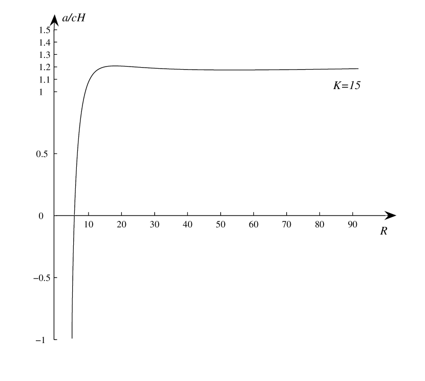
Figure 1: Represents the function $a_{p}/cH$ for Pioneer 10 as a function of the distance R measured in AU. K=15 corresponds that measuring the time started 235.5 days before the spacecraft was at the perihelion.

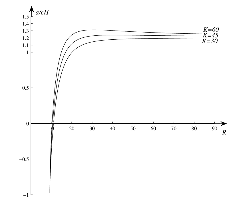
Figure 2: Represents the function $a_{p}/cH$ for Pioneer 11 as a function of the distance R measured in AU. K=30, 45, 60 corresponds that measuring the time started 323, 485, 647 days before the spacecraft was at the perihelion.

References

- Anderson et al. (1998) Anderson, J. D., Laing, P. A., Lau, E. L., Liu, A. S., Nieto, M. M., & Turyshev, S. G. 1998, Phys. Rev. Lett., 81, 2858, eprint: gr-qc/9808081.
- Anderson et al. (2002) Anderson, J. D., Laing, P. A., Lau, E. L., Liu, A. S., Nieto, M. M., & Turyshev, S. G. 2002, Phys. Rev. D, 65, 082004, eprint: gr-qc/0104064.
- Belayev (2001) Belayev, W. B. 2001, Space Subst., 7, 63, eprint: gr-qc/0110099.
- Bertolami et al. (2004) Bertolami, O., & Páramos, J. 2004, Class. & Quant. Grav., 21, 3309, eprint: gr-qc/0310101.
- Cadoni (2004) Cadoni, M. 2004, Gen. Rel. Grav., 36, 2681, eprint: gr-qc/0312054.
- Calchi et al. (2000) Calchi Novati, S., Capozziello, S., & Lambiase, G. 2000, Grav. Cosmol., 6, 173
- Capozzielo et al. (2001) Capozzielo, S., De Martino, S., De Siena, S., & Illuminati, F. 2001, Mod. Phys. Lett. A, 16, 693
- Consoli et al. (1999) Consoli, M., & Siringo, F. 1999, eprint: hep-ph/9910372.
- Crawford (1999) Crawford, D. F. 1999, Phys. Rev. Lett., submitted, eprint: astro-ph/9904150.
- Foot et al. (2001) Foot, R., & Volkas, R. R. 2001, Phys. Lett. B, 517, 13, eprint: gr-qc/0108051.
- Guruprasad (1999,2000) Guruprasad, V. 1999, eprint: astro-ph/9907363, 1999, eprint: gr-qc/0005014, 2000, eprint: gr-qc/0005090.
- Ingersoll et al. (1999) Ingersoll, P., Johnson, T. V., Kargel, J., Kirk, R., Didon, D. I. N., Perchoux, J., & Courtens, E. 1999, Preprint Universitée de Montpellier
- Iorio (2006) Iorio, L. 2006, New Astronomy, in press, eprint: gr-qc/0601055.
- Ivanov (2001) Ivanov, M. A. 2001, Gen. Rel. Grav., 33 479, eprint: astro-ph/0005084.
- Kaspi et al. (1994) Kaspi, V. M., Taylor, J. H., & Ryba, M. F. 1994, ApJ, 428, 713
- Mbelek et al. (1999) Mbelek, J. P., & Lachièze-Rey, M. 1999, Phys. Rev. D, submitted, eprint: gr-qc/9910105.
- Milgrom (2001) Milgrom, M. 2001, Acta Phys. Pol. B, 32, 3613
- Modanese (1999) Modanese, G. 1999, Nucl. Phys. B, 556, 397, eprint: gr-qc/9903085.
- Manyaneza et al. (1999) Munyaneza, F., & Viollier, R. D. 1999, eprint: astro-ph/9910566.
- Nottale (2003) Nottale, L. 2003, eprint: gr-qc/0307042.
- Ostvang (2002) Ostvang, D. 2002, Class. & Quant. Grav., 19, 4131, eprint: gr-qc/9910054.
- Ranada (2005) Rañada, A. F. 2005, Found. Phys., 34, 1955, eprint: gr-qc/0403013, gr-qc/0410084.
- Rosales et al. (1999) Rosales, J. L., & Sánchez-Gomez, J. L. 1999, eprint: gr-qc/9810085.
- Sidharth (2000) Sidharth, B. G. 2000, Nuovo Cim. B, 115, 151, eprint: astro-ph/9905052.
- Stairs et al. (1998) Stairs, I. H., Arzoumanian, Z., Camilo, F., Lyne, A. G., Nice, D. J., Taylor, J. H., Thorsett, S. E., & Wolszczan, A. 1998, ApJ, 505, 352, eprint: astro-ph/9712296.
- Stairs et al. (2002) Stairs, I. H., Thorsett, S. E., Taylor, J. H., & Wolszczan, A. 2002, ApJ, 581, 501, eprint: astro-ph/0208357.
- Trencevski (2005a) Trenčevski, K. 2005a, Gen. Rel. Grav., 37 (3), 507, eprint: gr-qc/0402024, gr-qc/0403067.
- Trencevski (2005b) Trenčevski, K. in Int. Conf. on Geometry and Related Topics, Belgrade, June 26 - July 2, 2005b, in press
- Trencevski (2006) Trenčevski, K. 2006, in Trends in Pulsar Research, ed. J.A.Lowry (New York: Nova Science), in press
- Turyshev et al. (2006) Turyshev, S. G., Toth, V. T., Kellog, L. R., Lau, E. L., & Lee, K. J. 2006, Int. J. Mod. Phys. D, 15, 1, eprint: gr-qc/0512121.
- Turyshev et al. (2004) Turyshev, S. G., Nieto, M. M., & Anderson, J. D. 2004, in The XXII Texas Symposium on Relativistic Astrophysics, Stanford Univ., December 13-17, 2004, eprint: gr-qc/0503021.
- Turyshev et al. (2005) Turyshev, S. G., Nieto, M. M., & Anderson, J. D. in XXIst IAP Colloquium on ”Mass Profiles and Shopes of Cosmological Structures”, Paris, July 4-9, 2005, eprint: gr-qc/0510081.
- Wood et al. (2001) Wood, J., & Moreau, W. 2001, eprint: gr-qc/0102056.