Half century of black-hole theory:
from physicists’ purgatory to mathematicians’ paradise.

Abstract: Although implicit in the discovery of the Schwarzschild solution 40 years earlier, the issues raised by the theory of what are now known as black holes were so unsettling to physicists of Einstein’s generation that the subject remained in a state of semiclandestine gestation until his demise. That turning point – just half a century after Einstein’s original foundation of relativity theory, and just half a century ago today – can be considered to mark the birth of black hole theory as a subject of systematic development by physicists of a new and less inhibited generation, whose enthusastic investigations have revealed structures of unforeseen mathematical beauty, even though questions about the physical significance of the concomitant singularities remain controversial.

1. Introduction: Schwarzschild’s unwelcome solution.

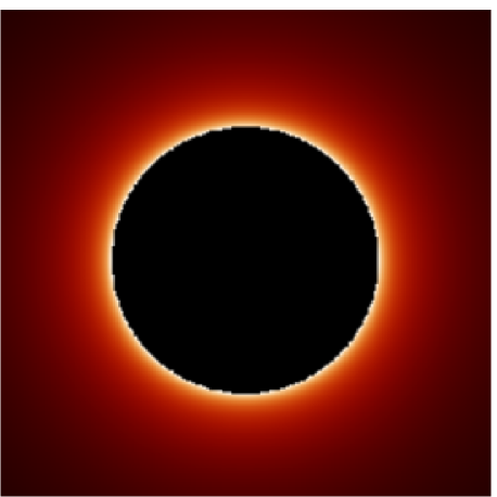
Figure 1: Numerically simulated view of (isolated) spherical black hole illuminated only by uniform distant sky background from which light is received only for viewing angle ${\color[rgb]{0.8,0.2,0}\alpha}>{\color[rgb]{0.8,0.2,0}\beta}$ where, for an observer falling radially from rest at large distance, the angle ${\color[rgb]{0.8,0.2,0}\beta}$ subtended by the hole will be given by the formula (45) obtained in the appendix.

This illustrated review is intended to provide a brief overview of the emergence, during the last half century, of the theory of ordinary (macroscopic 4-dimensional) black holes, considered as a phenomenon that (unlike the time reversed phenomenon of white holes) is manifestly of astrophysical importance in the real world. The scope of this review therefore does not cover quantum aspects such as the Bekenstein-Hawking particle creation effect, which is far too weak to be significant for the macroscopic black holes that are believed to actually exist in the observable universe. Nor does it cover the interesting mathematics of higher dimensional generalisations, a subject that is (for the time being) so far from relevance to the known physical world (in which – according to the second law of thermodynamics – the distinction between past and future actually matters) that its practitioners have formed a subculture in which the senior members seem to have forgotten (and their juniors seem never to have been aware of have been aware of) the distinction between black and white holes, as they have adopted a regretably misleading terminology whereby the adjective “black” is abusively applied to any brane system that is hollow – including the case of an ordinary (black or white) hole, which, to be systematic, should be classified as a (black or white) hollow zero brane of codimension 3.

The rapid general acceptance of the reality and importance of the positrons whose existence was implied by Dirac’s 1928 theory of the electron is in striking contrast with the widespread resistance to recognition of the reality and importance of the black holes whose existence was implied by Einstein’s 1915 theory of gravity. It is symptomatic that black holes were not even named as such until more than half a century later. The sloth with which the subject has been developed over the years is illustrated by the fact that although the simplest black hole solution was already discovered (by Schwarzschild) in 1916, the simulation in Figure 1 of the present review (80 years later) provides what seems to the first serious reply to the very easy question of what it would actually look like, all by itself, with no illumination other than that from a uniform sky background.

Much of the responsibility for the delay in the investigation of the consequences of his own theory is attributable [1] to Einstein himself. Although his work had revolutionary implications, Einstein’s instincts tended to be rather conservative. It was as a matter of necessity (to provide an adequate account first of electromagnetism and then of gravitation) rather than preference that Einstein introduced the radically new paradigms involved first in his theory of special relativity, just a hundred years ago, and then in the work on general relativity that came to fruition ten years later. When cherished prejudices were undermined by the consequences, Einstein was as much upset as any of his contempory colleagues. It could have been said of Albert Einstein (as it was said of his illustrious and like minded contempory, Arthur Eddington) that he was always profound, but sometimes profoundly wrong.

The most flagrant example was occasionned by Friedmann’s prescient 1922 discovery of what is now known as the “big bang” solution of the general relativity equations, which Einstein refused to accept because it conflicted with his unreasonable prejudice in favor of a cosmological scenario that would be not only homogeneous (as actually suggested by subsequently available data) but also static (as commonly supposed by earlier generations) despite the incompatibility (in thermal disequilibrium) of these alternative simplifications with each other and with the obvious observational consideration (known in cosmologically minded circles as the Cheseaux-Olbers paradox) that – between the stars – the night sky is dark. Einstein’s incoherent attitude (reminiscent of the murder suspect who claimed to have an alibi as well as the excuse of having acted in self defense) lead him not only to tamper with his own gravitation equations by inclusion of the cosmological constant, but anyway to presume without checking that Friedmann’s (actually quite valid) solution of the original version must have been mathematically erroneous.

Compared with his tendency to obstruct progress in cosmology, Einstein’s conservatism was rather more excusible in the not so simple case of what are now known as black holes. It is understandable that (like Eddington) he should have been unwilling to explore the limitations on the validity of his theory that are indicated by the weird and singular – or as Thorne [1] puts it “outrageous” – features that emerge when strong field solutions of the general relativity equations are extrapolated too far into the non linear regime.

Figure 2: John Wheeler with Robert Dicke (Princeton 1971).

At the outset Einstein’s interest in the spherical vacuum solution of his 1915 gravitational field equations was entirely restricted to the weak field regime, far outside the “horizon” at ${\color[rgb]{0,0.6,0.2}r}=2{\color[rgb]{0.6,0.2,0.0}m}$ in the simple exact solution

$${\rm d}s^{2}={\color[rgb]{0,0.6,0.2}r}^{2}({\rm d}{\color[rgb]{0.8,0.2,0}\theta}^{2}+{\rm sin}^{2}{\color[rgb]{0.8,0.2,0}\theta}\,{\rm d}{\color[rgb]{0.3,0.0,0.8}\phi}^{2})+{\rm d}{\color[rgb]{0,0.6,0.2}r}^{2}/(1\!-\!{2{\color[rgb]{0.6,0.2,0.0}m}}/{{\color[rgb]{0,0.6,0.2}r}})-(1\!-\!{2{\color[rgb]{0.6,0.2,0.0}m}}/{{\color[rgb]{0,0.6,0.2}r}}){\rm d}{\color[rgb]{0.3,0.0,0.8}t}^{2}\!\,,$$ (1)

that was obtained within a year, but that was immediately orphanned by the premature death of its discoverer, Karl Schwarszschild, after which its embarrassing physical implications were hardly taken seriously by anyone – with the notable exception of Oppenheimer [2] – until the topic was taken up by a less inhibited generation subsequent to the death of Einstein himself, just half a century ago, at Princeton in 1955. It was only then (and there) that John Wheeler inaugurated the systematic development of the subject – for which he coined the name “black hole” theory – in a series of pionnering investigations that started [3] by addressing the crucial question of stability, while not long afterwards, on the other side of the “iron curtain” another nuclear arms veteran, Yacob Zel’dovich, initiated an independent approach [4] to the same problem (using the alternative name “frozen star” which in the end did not catch on).

2. Outcome of stellar evolution: Chandra’s unwelcome limit.

The question of gravitational trapping of light had been raised in the eighteenth century by Michel and Laplace, whose critical mass ${\color[rgb]{0.6,0.2,0.0}m}\approx{\color[rgb]{0.6,0.2,0.0}\rho}^{-1/2}$ assumed the standard mass density that is understood (on the basis of quantum theory as developped by 1930) to result in hadronic matter from balance between Fermi repulsion and electrostatic attraction which (in Planck units, with proton and electron masses ${\color[rgb]{0.6,0.2,0.0}m}_{\rm p}\approx 10^{-19}$ , ${\color[rgb]{0.6,0.2,0.0}m}_{\rm e}\approx 10^{-22}$ gives ${\color[rgb]{0.6,0.2,0.0}\rho}\approx{\color[rgb]{0.6,0.2,0.0}m}_{\rm p}{\color[rgb]{0,0.6,0.2}n}$ with ${\color[rgb]{0,0.6,0.2}n}\approx\lambda^{-3}$ for the Bohr radius $\lambda\approx{\color[rgb]{0.8,0.2,0}e}^{2}/{\color[rgb]{0.6,0.2,0.0}m}_{\rm e}$ with ${\color[rgb]{0.8,0.2,0}e}^{2}\simeq 1/137$ . However most theorists refused to face the issue of gravitational collapse even after progress in quantum theory lead to Chandrasekhar’s 1931 discovery of the maximum mass ${\color[rgb]{0.6,0.2,0.0}m}\approx{\color[rgb]{0.6,0.2,0.0}m}_{\rm p}^{-2}$ for cold body – which is attained when relativistic gas pressure ${\color[rgb]{0.6,0.2,0.0}P}\approx{\color[rgb]{0,0.6,0.2}n}/\lambda\approx{\color[rgb]{0,0.6,0.2}n}^{4/3}$ provides the support required by virial condition ${\color[rgb]{0.6,0.2,0.0}P}\approx{\color[rgb]{0.6,0.2,0.0}m}_{\rm p}^{2/3}{\color[rgb]{0.6,0.2,0.0}\rho}^{4/3}$ .

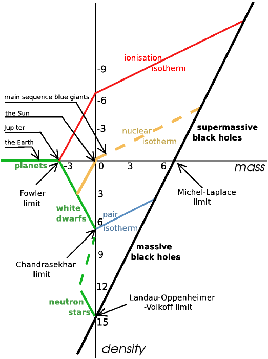
Figure 3: Logarithmic plot of density versus mass

For a lower mass ${\color[rgb]{0.6,0.2,0.0}m}\mathrel{\hbox to0.0pt{\lower 3.0pt\hbox{$\mathchar 536\relax$}\hss}\raise 2.0pt\hbox{$\mathchar 316\relax$}}{\color[rgb]{0.6,0.2,0.0}m}_{\rm p}^{-2}$ , stellar evolution at finite temperature ${\color[rgb]{0.8,0.4,0.0}\Theta},$ with gas pressure ${\color[rgb]{0.6,0.2,0.0}P}\approx{\color[rgb]{0,0.6,0.2}n}{\color[rgb]{0.8,0.4,0.0}\Theta}$ subject to ${\color[rgb]{0.6,0.2,0.0}\rho}\approx{\color[rgb]{0.8,0.4,0.0}\Theta}^{3}/{\color[rgb]{0.6,0.2,0.0}m}_{\rm p}^{\,3}{\color[rgb]{0.6,0.2,0.0}m}^{2}$ , can terminate in cold equilibrium supported by non-relativistic Fermi pressure ${\color[rgb]{0.6,0.2,0.0}P}\approx{\color[rgb]{0,0.6,0.2}n}^{5/3}/{\color[rgb]{0.6,0.2,0.0}m}_{\rm e}$ giving ${\color[rgb]{0.6,0.2,0.0}\rho}\approx{\color[rgb]{0.6,0.2,0.0}m}_{\rm e}^{\,3}{\color[rgb]{0.6,0.2,0.0}m}_{\rm p}^{\,5}{\color[rgb]{0.6,0.2,0.0}m}^{2}$ for a white dwarf, or ${\color[rgb]{0.6,0.2,0.0}P}\approx{\color[rgb]{0,0.6,0.2}n}^{5/3}/{\color[rgb]{0.6,0.2,0.0}m}_{\rm p}$ giving ${\color[rgb]{0.6,0.2,0.0}\rho}\approx{\color[rgb]{0.6,0.2,0.0}m}_{\rm p}^{\,8}{\color[rgb]{0.6,0.2,0.0}m}^{2}$ for neutron star, as shown in Figure 3.

However a self gravitating mass of hot gas will be radiation dominated with ${\color[rgb]{0.6,0.2,0.0}P}\approx{\color[rgb]{0.8,0.4,0.0}\Theta}^{4}$ , whenever its mass exceeds the Chandrasekhar limit, ${\color[rgb]{0.6,0.2,0.0}m}\mathrel{\hbox to0.0pt{\lower 3.0pt\hbox{$\mathchar 536\relax$}\hss}\raise 2.0pt\hbox{$\mathchar 318\relax$}}{\color[rgb]{0.6,0.2,0.0}m}_{\rm p}^{-2},$ so that, as first understood by Chandra’s Cambridge research director, Arthur Eddington, its condition for (thermally supported) equilibrium will be given by ${\color[rgb]{0.6,0.2,0.0}\rho}\approx{\color[rgb]{0.8,0.4,0.0}\Theta}^{3}/{\color[rgb]{0.6,0.2,0.0}m}^{1/2}.$ What Chandra could never get Eddington to accept is that, for such a large mass, no cold equilibrium state will be available, so after exhaustion of fuel for thermonuclear burning (at ${\color[rgb]{0.8,0.4,0.0}\Theta}\approx{\color[rgb]{0.8,0.2,0}e}^{4}{\color[rgb]{0.6,0.2,0.0}m}_{\rm p}$ ) gravitational collapse will become inevitable.

3. Spherical collapse past the horizon

Eddington’s example shows how, as has described in detail by Werner Israel [5] (and in striking contrast with the open mindedness of Michel and Laplace a century and a half earlier) physicists of Einstein’s generation tried to convince themselves that nature would never allow compacification within a radius comparable to the Schwarzschild value. While Einstein lived, even after Chandrasekhar’s discovery had shown that such a fate might often be difficult to avoid, the implications were taken seriously only by Oppenheimer and his colleagues, who showed [2] how, as shown in Figure 4, the solutions of Schwarzschild and Friedmann could be combined to provide a complete description of the collapse of a homogeneous spherical body through what is now called its event horizon all the way to a terminal singularity.

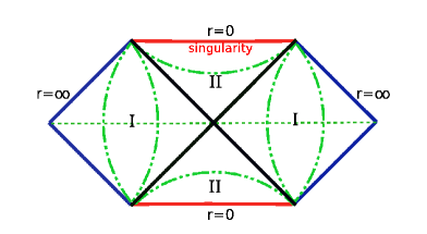
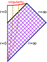
Figure 4: Conformal Projection diagrams showing firstly the combined black and white hole geometry obtained (belatedly [6] in 1960, by Wheeler in collaboration with Kruskal) as the artificial analytic (vacuum) extension of the Schwarzschild solution, and secondly a more astrophysically natural extension with homogeneous interior (found in 1939 [2] by Oppenheimer in collaboration with Sneyder) in which the shaded egion is the “domain of outer communications” and the unshaded region is the prototype example of a hole qualifiable as black in the strict sense.

Despite the persuasion of such experienced physicists as Wheeler and Zel’dovich, and the mathematical progress due to younger geometers such as Robert Boyer and particularly Roger Penrose, the astrophysical relevance of the region near and within the horizon continued to be widely disbelieved until (and even after) the 1967 discovery [7] by Israel of the uniqueness of the Schwarzschild geometry as a static solution: many people (for a while including Israel himself [5]) still supposed (wrongly) that the horizon was an unstable artefact of exact spherical symmetry. It is therefore not surprising that the question of what such a black hole would actually look like was not addressed until much more recently, particularly considering that nothing would be seen at all without some source of illumination.

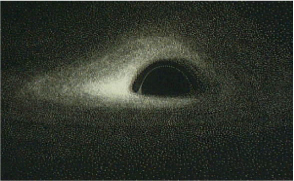
Figure 5: First realistic simulation of distant view of spherical black hole with thin accretion disc by Jean-Pierre Luminet, 1978.

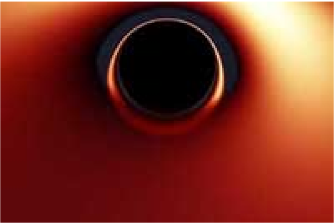
Figure 6: Simulation of close up view of spherical black hole with thin accretion disc by Jean Alain Marck, 1996.

The realisation that many spectacular astrophysical phenomena ranging in scale from supermassive quasars in distant parts of the universe down to stellar mass X ray sources within our own galaxy may be attributed to accretion discs [8, 9, 10] round more or less massive black holes has however provided the motivation for increasingly realistic numerical simulations (Figures 5 and 6) of what would be seen from outside in the presence of an illuminating source of this kind [11, 12].

As the most easily calculable example, I have shown in the appendix how to work out the case shown in Figure 1 of an isolated spherical black hole for which the only source of illumination is a uniform distant sky background, viewed as a function of proper time,

$$\tau=-\frac{4{\color[rgb]{0.6,0.2,0.0}m}}{3}\left(\frac{{\color[rgb]{0,0.6,0.2}r}}{2{\color[rgb]{0.6,0.2,0.0}m}}\right)^{3/2}\,,$$ (2)

by a (doomed) observer falling towards the singularity inside the black hole, with zero energy and angular momentum.

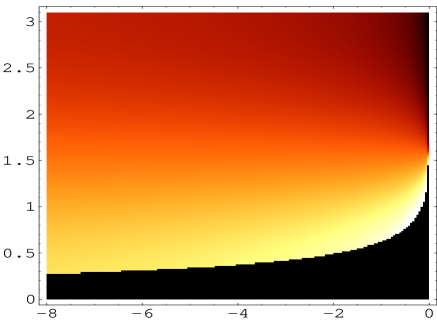
Figure 7: Plot of reception angle ${\color[rgb]{0.8,0.2,0}\alpha}$ against countdown proper time $\tau$ for arrival at singularity of radially falling zero-energy observer in units such that $2{\color[rgb]{0.6,0.2,0.0}m}=\sqrt{2/3}$ so that null orbit radius ${\color[rgb]{0,0.6,0.2}r}=3{\color[rgb]{0.6,0.2,0.0}m}$ is crossed when $\tau=-1.$ Constant brightness contours indicate intensity of light received from uniform background, which will be inversely proportional to 4th power of redshift factor $(1+Z)$ , having unshifted value for rays arriving at angle $\pi/2$ .

In such a case the redshift $Z$ determining the observed energy ${\color[rgb]{0.6,0.2,0.0}{\cal E}}/(1+Z)$ of a photon emitted from the sky background with the uniform average energy ${\color[rgb]{0.6,0.2,0.0}{\cal E}}$ say will be given by the formula

$$Z=-\frac{{\rm cos}\,{\color[rgb]{0.8,0.2,0}\alpha}}{\sqrt{{\color[rgb]{0,0.6,0.2}r}/2{\color[rgb]{0.6,0.2,0.0}m}}}\,,\hskip 28.45274pt{\color[rgb]{0.8,0.2,0}\alpha}>{\color[rgb]{0.8,0.2,0}\beta}\,,$$ (3)

where ${\color[rgb]{0.8,0.2,0}\alpha}$ is the apparent angle of reception, which must of course excede the apparent angle ${\color[rgb]{0.8,0.2,0}\beta}$ subtended by the black hole. This means that the redshift will be positive (so that the sky will appear darker than normal) due to the Doppler effect, for photons coming in from behind the observer (with ${\color[rgb]{0.8,0.2,0}\alpha}>\pi/2$ ). However photons received in the range ${\color[rgb]{0.8,0.2,0}\beta}<{\color[rgb]{0.8,0.2,0}\alpha}<\pi/2$ will be blueshifted by an amount that will diverge, as shown in Figure 7, as the singularity is approached.

4. Discovery of horizon stability and of Kerr solution

Following the demise of Einstein (and the development of nuclear weapons) a new (less inhibited) generation of physicists, lead by Wheeler and Zel’dovich, came to recognise the likelihood – and need in any case for testing – of stability with respect to non-spherical perturbations of what was termed a “black hole”. Work by Vishweshwara [13], Price [14], and others confirmed that “anything that can be radiated away will be radiated away” – leaving a final equilibrium state characterised only by mass and angular momentum. The (still open) mathematical question of the extent to which this remains true (with singularities hidden inside horizon) for very large deviations from sphericity was raised by the “cosmic censorship” conjecture formulated by Roger Penrose [15, 16] but in any case the relevance of black holes for astrophysical phenomena (notably quasars) was generally accepted in astronomical circles from 1970 onwards.

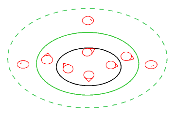
Figure 8: Sketch showing projections of null cones in equatorial space section of Kerr metric. The pale curve marks the “ergosurface” bounding the region where stationary motion is allowed, and the heavy black curve marks the horizon bounding the trapped “black hole” region.

The generic form of what was afterwards recognised to be the final black hole equilibrium state state in question was discovered in 1963, when Roy Kerr announced [17, 18] that “among the solutions … there is one which is stationary … and also axisymmetric. Like the Schwarzschild metric, which it contains, it is type D … ${\color[rgb]{0.6,0.2,0.0}m}$ is a real constant … The metric is

$${\rm d}s^{2}=({\color[rgb]{0,0.6,0.2}r}^{2}+{\color[rgb]{0.6,0.2,0.0}a}^{2}{\rm cos}^{2}{\color[rgb]{0.8,0.2,0}\theta})({\rm d}{\color[rgb]{0.8,0.2,0}\theta}^{2}+{\rm sin}^{2}{\color[rgb]{0.8,0.2,0}\theta}\,{\rm d}{\color[rgb]{0.3,0.0,0.8}\phi}^{2})+2({\rm d}{\color[rgb]{0.3,0.0,0.8}u}+{\color[rgb]{0.6,0.2,0.0}a}\,{\rm sin}^{2}{\color[rgb]{0.8,0.2,0}\theta}\,{\rm d}{\color[rgb]{0.3,0.0,0.8}\phi})({\rm d}{\color[rgb]{0,0.6,0.2}r}+{\color[rgb]{0.6,0.2,0.0}a}\,{\rm sin}^{2}{\color[rgb]{0.8,0.2,0}\theta}\,{\rm d}{\color[rgb]{0.3,0.0,0.8}\phi})$$

$$-\!\left(1-\!\frac{2{\color[rgb]{0.6,0.2,0.0}m}{\color[rgb]{0,0.6,0.2}r}}{{\color[rgb]{0,0.6,0.2}r}^{2}\!+\!{\color[rgb]{0.6,0.2,0.0}a}^{2}{\rm cos}^{2}{\color[rgb]{0.8,0.2,0}\theta}}\right)\!({\rm d}{\color[rgb]{0.3,0.0,0.8}u}+{\color[rgb]{0.6,0.2,0.0}a}\,{\rm sin}^{2}{\color[rgb]{0.8,0.2,0}\theta}\,{\rm d}{\color[rgb]{0.3,0.0,0.8}\phi})^{2}\,,$$ (4)

where ${\color[rgb]{0.6,0.2,0.0}a}$ is a real constant. This may be transformed to an asymptotically flat coordinate system … we find that ${\color[rgb]{0.6,0.2,0.0}m}$ is the Schwarzschild mass and ${\color[rgb]{0.6,0.2,0.0}m}{\color[rgb]{0.6,0.2,0.0}a}$ the angular momentum ”.

Since the black hole concept had still not been clearly formulated then, it was at first (wrongly) supposed that the physical relevance of this vacuum solution would be as the exterior to a compact self gravitating body like a neutron star, as suggested by Kerr’s (off the mark) conclusion [17] that it would be “desirable to calculate an interior solution.”

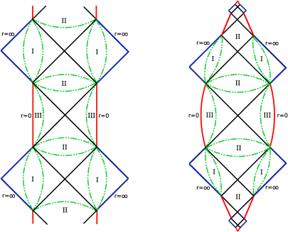
Figure 9: Representation of equatorial space-time section of Kerr metric by Conformal Projection diagrams. (Such C.P. diagrams were originally developed for this purpose.) The second version achieves complete compactifiction by letting scale for successive universes tend to zero at extremities of chain.

What actually makes the Kerr metric so important however, as can be see from Figure 9 (using C.P. diagrams, which were originally developed for this purpose) is the feature first clearly recognised [19, 20] by Bob Boyer in 1965, which is that for ${\color[rgb]{0.6,0.2,0.0}a}^{2}\leq{\color[rgb]{0.6,0.2,0.0}m}^{2}$ the distant sky limit known as “asymptopia” is both visible and accessible only in a non-singular “domain of outer communications” bounded by past and future null (outer) horizons, on which ${\color[rgb]{0,0.6,0.2}\Delta}=0,$ where

$${\color[rgb]{0,0.6,0.2}r}={\color[rgb]{0.6,0.2,0.0}m}+{\color[rgb]{0.6,0.2,0.0}c}\,,\hskip 28.45274pt{\color[rgb]{0.6,0.2,0.0}c}=\sqrt{{\color[rgb]{0.6,0.2,0.0}m}^{2}-{\color[rgb]{0.6,0.2,0.0}a}^{2}}$$ (5)

.

The topology within the black (and white) hole regions was first elucidated [21] in terms of Conformal Projections on the symmetry axis in 1966 and then completely [22, 23, 24] by Boyer, Lindquist and myself in 1967 and 1968 – the year when the much needed term “black hole” was finally introduced by Wheeler to describe the region from which light cannot escape to “asymptopia”. (A “white hole” region would be one that could not receive light from“asymptopia”.) In the generic rotating case (unlike the static Schwarzschild limit) the well behaved domain outside the black hole horizon includes an “ergosphere” region where, as shown in Figure 8, the Killing vector generating the stationarity symmetry becomes spacelike, so that (globally defined) particle energies can be negative.

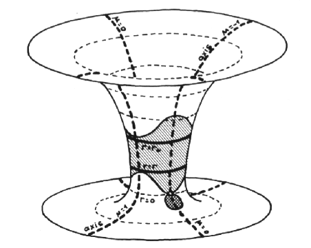
Figure 10: Reproduction from 1972 Les Houches notes [24]: sketch of $\{{\color[rgb]{0,0.6,0.2}r},{\color[rgb]{0.8,0.2,0}\theta}\}$ section through ring singularity at junction between heavily shaded region responsible for causality violation where axisymmetry generator is spacelike, and lightly shaded ergo region where time summetry generator is spacelike.

In contrast with the good behavior of the outer region, ${\color[rgb]{0,0.6,0.2}r}>{\color[rgb]{0.6,0.2,0.0}m}+{\color[rgb]{0.6,0.2,0.0}c},$ I found that, as well as having the irremovable ring shaped curvature singularity already noticed by Kerr where ${\color[rgb]{0,0.6,0.2}r}^{2}\!+\!{\color[rgb]{0.6,0.2,0.0}a}^{2}{\rm cos}^{2}{\color[rgb]{0.8,0.2,0}\theta}\!\rightarrow\!0,$ , the inner parts of the rotating Kerr solutions would always be causally pathological, due to the existence near the ring singularity of a small region (see Figure 10) where the axial symmetry generating Killing vector becomes timelike[23, 25]. This feature gives rise to a causality violating “time machine region” (a feature so “outrageous” as to be unmentionable even by Thorne [1]) that would extend all the way out to “asymptopia” (meaning ${\color[rgb]{0,0.6,0.2}r}\rightarrow+\infty$ ) in the – presumably unphysical – case for which ${\color[rgb]{0.6,0.2,0.0}a}^{2}>{\color[rgb]{0.6,0.2,0.0}m}^{2}$ . (I would emphasize that this kind of time machine, like those recently considered by Ori [32], would survive even if one takes the covering space, unlike a time machine of the wormhole kind discussed by Thorne [1] which is merely an artefact of multiply connected space time topology).

In so far as the (physically relevant) black hole cases characterised by ${\color[rgb]{0.6,0.2,0.0}a}^{2}\leq{\color[rgb]{0.6,0.2,0.0}m}^{2}$ are concerned, the good news [23, 25] (for believers in causality) is that the closed timelike lines are all contained within the inner region ${\color[rgb]{0,0.6,0.2}r}<{\color[rgb]{0.6,0.2,0.0}m}-{\color[rgb]{0.6,0.2,0.0}c}.$ The boundary of the time machine region is constituted by the “inner horizon”, where ${\color[rgb]{0,0.6,0.2}r}={\color[rgb]{0.6,0.2,0.0}m}-{\color[rgb]{0.6,0.2,0.0}c}.$ which acts as a Cauchy hypersuface from the point of view of inital data for formation of the black hole by gravitational collapse. Unlike the outer horizon ${\color[rgb]{0,0.6,0.2}r}={\color[rgb]{0.6,0.2,0.0}m}+{\color[rgb]{0.6,0.2,0.0}c},$ whose stability throughout the allowed range $0\leq{\color[rgb]{0.6,0.2,0.0}a}^{2}<{\color[rgb]{0.6,0.2,0.0}m}^{2}$ has been even confirmed by Whiting [26], it was to be expected [27, 28] that a Cauchy horizon of the kind occurring at ${\color[rgb]{0,0.6,0.2}r}={\color[rgb]{0.6,0.2,0.0}m}-{\color[rgb]{0.6,0.2,0.0}c}$ would be unstable, and it has been shown that outcome is likely to be the formation of a curvature singularity of the weak kind designated by the term “mass inflation” [29, 30, 31].

5. Seductive mathematical features of Kerr type metrics

In his original 1963 letter [17], and with Alfred Schild [18] in a sequel, Kerr obtained the useful alternative form

$${\rm d}s^{2}=g_{\mu\nu}\,{\rm d}x^{\mu}{\rm d}x^{\nu}=\eta_{\mu\nu}+2({\color[rgb]{0.6,0.2,0.0}m}/{\color[rgb]{0.4,0,0.4}U}){\color[rgb]{0.4,0,0.4}n}_{\mu}{\color[rgb]{0.4,0,0.4}n}_{\nu}$$ (6)

with null covector ${\color[rgb]{0.4,0,0.4}n}_{\mu}{\rm d}x^{\mu}\!={\rm d}{\color[rgb]{0.3,0.0,0.8}u}+{\color[rgb]{0.6,0.2,0.0}a}\,{\rm sin}^{2}{\color[rgb]{0.8,0.2,0}\theta}\,{\rm d}{\color[rgb]{0.3,0.0,0.8}\phi}\,,$ for ${\color[rgb]{0.4,0,0.4}U}=({\color[rgb]{0,0.6,0.2}r}^{2}+{\color[rgb]{0.6,0.2,0.0}a}^{2}{\rm cos}^{2}{\color[rgb]{0.8,0.2,0}\theta})/{\color[rgb]{0,0.6,0.2}r}\,,$ in a flat background. The latter was obtained in the Minkowski form,

$$\eta_{\mu\nu}\,{\rm d}x^{\mu}{\rm d}x^{\nu}={\rm d}\bar{\color[rgb]{0.4,0,0.4}x}^{2}\!+\!{\rm d}\bar{\color[rgb]{0.4,0,0.4}y}^{2}\!+\!{\rm d}\bar{\color[rgb]{0.4,0,0.4}z}^{2}\!-{\rm d}\bar{\color[rgb]{0.3,0.0,0.8}t}^{2}\,,$$ (7)

by setting $\bar{\color[rgb]{0.3,0.0,0.8}t}={\color[rgb]{0.3,0.0,0.8}u}-{\color[rgb]{0,0.6,0.2}r}\,,$ $\bar{\color[rgb]{0.4,0,0.4}z}={\color[rgb]{0.6,0.2,0.0}a}\,{\rm cos}\,{\color[rgb]{0.8,0.2,0}\theta}\,,$ $\bar{\color[rgb]{0.4,0,0.4}x}+i\bar{\color[rgb]{0.4,0,0.4}y}=({\color[rgb]{0,0.6,0.2}r}-i{\color[rgb]{0.6,0.2,0.0}a}){\rm e}^{i{\color[rgb]{0.3,0.0,0.8}\phi}}{\rm sin}\,{\color[rgb]{0.8,0.2,0}\theta}\,,$ which gave

$${\color[rgb]{0.4,0,0.4}n}_{\mu}{\rm d}x^{\mu}\!={\rm d}\bar{\color[rgb]{0.3,0.0,0.8}t}+\!\frac{\bar{\color[rgb]{0.4,0,0.4}z}{\rm d}\bar{\color[rgb]{0.4,0,0.4}z}}{{\color[rgb]{0,0.6,0.2}r}}\!+\frac{({\color[rgb]{0,0.6,0.2}r}\bar{\color[rgb]{0.4,0,0.4}x}\!-\!{\color[rgb]{0.6,0.2,0.0}a}\bar{\color[rgb]{0.4,0,0.4}y}){\rm d}\bar{\color[rgb]{0.4,0,0.4}x}\!+\!({\color[rgb]{0,0.6,0.2}r}\bar{\color[rgb]{0.4,0,0.4}y}\!+\!{\color[rgb]{0.6,0.2,0.0}a}\bar{\color[rgb]{0.4,0,0.4}x}){\rm d}\bar{\color[rgb]{0.4,0,0.4}y}}{{\color[rgb]{0,0.6,0.2}r}^{2}+{\color[rgb]{0.6,0.2,0.0}a}^{2}}\,.$$ (8)

(This form of pure vacuum solution was generalised to higher dimensions by Myers and Perry[33]. It is perhaps of greater current cosmological interest – in view of the evidence that the expansion of the universe is accelerating – that this form has also beeen extended to include a cosmological constant in a 4 dimensional De Sitter background by myself [24, 34], while further generalisations to a De Sitter background in 5 and higher dimensions [35, 36] have been obtained more recently.)

As well as time and axial symmmetry, the Kerr solution has a discrete PT symmetry that was predictable from Papapetrou’s “circularity” theorem [37], and made manifest in 1967 [22] by the Boyer Lindquist transformation

$${\rm d}{\color[rgb]{0.3,0.0,0.8}t}={\rm d}{\color[rgb]{0.3,0.0,0.8}u}-({\color[rgb]{0,0.6,0.2}r}^{2}+{\color[rgb]{0.6,0.2,0.0}a}^{2}){\color[rgb]{0,0.6,0.2}\Delta}^{-1}{\rm d}{\color[rgb]{0,0.6,0.2}r}\,,\ \ {\rm d}{\color[rgb]{0.3,0.0,0.8}\varphi}=-{\rm d}{\color[rgb]{0.3,0.0,0.8}\phi}+{\color[rgb]{0.6,0.2,0.0}a}\,{\color[rgb]{0,0.6,0.2}\Delta}^{-1}{\rm d}{\color[rgb]{0,0.6,0.2}r}\,,$$ (9)

with

$${\color[rgb]{0,0.6,0.2}\Delta}={\color[rgb]{0,0.6,0.2}r}^{2}-2{\color[rgb]{0.6,0.2,0.0}m}{\color[rgb]{0,0.6,0.2}r}+{\color[rgb]{0.6,0.2,0.0}a}^{2}\,.$$ (10)

This gives Kerr’s null form as

$${\color[rgb]{0.4,0,0.4}n}_{\mu}{\rm d}x^{\mu}\!={\rm d}{\color[rgb]{0.3,0.0,0.8}t}-{\color[rgb]{0.6,0.2,0.0}a}\,{\rm sin}^{2}{\color[rgb]{0.8,0.2,0}\theta}\,{\rm d}{\color[rgb]{0.3,0.0,0.8}\varphi}+{\color[rgb]{0.4,0,0.4}\varrho}^{2}{\color[rgb]{0,0.6,0.2}\Delta}^{-1}{\rm d}{\color[rgb]{0,0.6,0.2}r}\,,\hskip 28.45274pt{\color[rgb]{0.4,0,0.4}\varrho}\!=\!\sqrt{\!{\color[rgb]{0,0.6,0.2}r}^{2}\!+\!{\color[rgb]{0.6,0.2,0.0}a}^{2}{\rm cos}^{2}{\color[rgb]{0.8,0.2,0}\theta}},.$$ (11)

The metric itself is thereby obtained in the convenient form

$${\rm d}s^{2}={\color[rgb]{0.4,0,0.4}\varrho}^{2}\left(\frac{{\rm d}{\color[rgb]{0,0.6,0.2}r}^{2}}{{\color[rgb]{0,0.6,0.2}\Delta}}+{\rm d}{\color[rgb]{0.8,0.2,0}\theta}^{2}\right)+({\color[rgb]{0,0.6,0.2}r}^{2}+{\color[rgb]{0.6,0.2,0.0}a}^{2}){\rm sin}^{2}{\color[rgb]{0.8,0.2,0}\theta}\,{\rm d}{\color[rgb]{0.3,0.0,0.8}\varphi}^{2}+\frac{2{\color[rgb]{0.6,0.2,0.0}m}{\color[rgb]{0,0.6,0.2}r}}{{\color[rgb]{0.4,0,0.4}\varrho}^{2}}({\rm d}{\color[rgb]{0.3,0.0,0.8}t}-{\color[rgb]{0.6,0.2,0.0}a}\,{\rm sin}^{2}{\color[rgb]{0.8,0.2,0}\theta}\,{\rm d}{\color[rgb]{0.3,0.0,0.8}\varphi})^{2}\!-{\rm d}{\color[rgb]{0.3,0.0,0.8}t}^{2}\,,$$ (12)

in which there are cross terms involving the non-ignorable differentials, ${\rm d}{\color[rgb]{0,0.6,0.2}r}$ and ${\rm d}{\color[rgb]{0.8,0.2,0}\theta}\,,$ but – as the price for this simplification – if ${\color[rgb]{0.6,0.2,0.0}a}^{2}\leq{\color[rgb]{0.6,0.2,0.0}m}^{2}$ there will be a removable coordinate singularity on the null “horizon” where ${\color[rgb]{0,0.6,0.2}\Delta}$ vanishes.

Whereas the possibility of making the foregoing simplification was predictable in advance, there was no reason to anticipate the discovery [23, 38] that, in addition to the ordinary “circular” symmetry generated by Killing vectors, ${\color[rgb]{0.3,0.0,0.8}k}^{\mu}\partial/\partial x^{\mu}=\partial/\partial{\color[rgb]{0.3,0.0,0.8}t}$ and ${\color[rgb]{0.3,0.0,0.8}h}^{\mu}\partial/\partial x^{\mu}=\partial/\partial{\color[rgb]{0.3,0.0,0.8}\varphi}\,,$ the Kerr metric would turn out to have the hidden symmetry that is embodied in the canonical tetrad

$$g_{\mu\nu}\!=\sum_{{}_{i=1}}^{\,{}_{3}}{\color[rgb]{0.4,0,0.4}\vartheta}^{\hat{i}}_{\,\mu}{\color[rgb]{0.4,0,0.4}\vartheta}^{\hat{i}}_{\nu}-\!{\color[rgb]{0.4,0,0.4}\vartheta}^{\hat{{}^{0}}}_{\mu}{\color[rgb]{0.4,0,0.4}\vartheta}^{\hat{{}^{0}}}_{\nu}\!$$ (13)

specified by

$${\color[rgb]{0.4,0,0.4}\vartheta}^{\hat{{}^{1}}}_{\mu}{\rm d}x^{\mu}\!=\!(\!{\color[rgb]{0.4,0,0.4}\varrho}/\sqrt{\!{\color[rgb]{0,0.6,0.2}\Delta}}){\rm d}{\color[rgb]{0,0.6,0.2}r}\,,\hskip 28.45274pt{\color[rgb]{0.4,0,0.4}\vartheta}^{\hat{{}^{2}}}_{\mu}{\rm d}x^{\mu}\!={\color[rgb]{0.4,0,0.4}\varrho}\,{\rm d}{\color[rgb]{0.8,0.2,0}\theta},$$ (14)

$$\frac{{\color[rgb]{0.4,0,0.4}\vartheta}^{\hat{{}^{3}}}_{\mu}{\rm d}x^{\mu}\!}{{\rm sin}\,{\color[rgb]{0.8,0.2,0}\theta}}=\frac{({\color[rgb]{0,0.6,0.2}r}^{2}\!+\!{\color[rgb]{0.6,0.2,0.0}a}^{2}){\rm d}{\color[rgb]{0.3,0.0,0.8}\varphi}\!-\!{\color[rgb]{0.6,0.2,0.0}a}{\rm d}{\color[rgb]{0.3,0.0,0.8}t}}{{\color[rgb]{0.4,0,0.4}\varrho}}\,,\ \ \frac{{\color[rgb]{0.4,0,0.4}\vartheta}^{\hat{{}^{0}}}_{\mu}{\rm d}x^{\mu}\!}{\sqrt{\color[rgb]{0,0.6,0.2}\Delta}}=\frac{{\rm d}{\color[rgb]{0.3,0.0,0.8}t}\!-\!{\color[rgb]{0.6,0.2,0.0}a}\,{\rm sin}^{2}{\color[rgb]{0.8,0.2,0}\theta}\,{\rm d}{\color[rgb]{0.3,0.0,0.8}\varphi}}{{\color[rgb]{0.4,0,0.4}\varrho}}\,.$$ (15)

In terms of this canonical tetrad, the Kerr-Schild form of the metric is expressible as

$$g_{\mu\nu}=\eta_{\mu\nu}\!+\!2{\color[rgb]{0.6,0.2,0.0}m}{\color[rgb]{0,0.6,0.2}r}({\color[rgb]{0.4,0,0.4}\vartheta}^{\hat{{}^{0}}}_{\mu}\!+\!{\color[rgb]{0.4,0,0.4}\vartheta}^{\hat{{}^{1}}}_{\mu})({\color[rgb]{0.4,0,0.4}\vartheta}^{\hat{{}^{0}}}_{\nu}\!+\!{\color[rgb]{0.4,0,0.4}\vartheta}^{\hat{{}^{1}}}_{\nu})\,,$$ (16)

while the Killing-Yano 2-form brought to light by Roger Penrose and his coworkers is expressible as

$${\color[rgb]{0.3,0.0,0.8}f}_{\mu\nu}=2{\color[rgb]{0.6,0.2,0.0}a}\,{\rm cos}\,{\color[rgb]{0.8,0.2,0}\theta}\,{\color[rgb]{0.4,0,0.4}\vartheta}^{\hat{{}^{1}}}_{[\mu}{\color[rgb]{0.4,0,0.4}\vartheta}^{\hat{{}^{0}}}_{\nu]}-2{\color[rgb]{0,0.6,0.2}r}\,{\color[rgb]{0.4,0,0.4}\vartheta}^{\hat{{}^{2}}}_{[\mu}{\color[rgb]{0.4,0,0.4}\vartheta}^{\hat{{}^{3}}}_{\nu]}\,.$$ (17)

The property of being a Killing-Yano 2-form means that it is such as to satisfy the very restrictive condition condition

$$\nabla_{\!\mu}{\color[rgb]{0.3,0.0,0.8}f}_{\nu\rho}=\nabla_{\![\mu}{\color[rgb]{0.3,0.0,0.8}f}_{\nu\rho]}\,,$$ (18)

thus providing a symmetric solution

$${\color[rgb]{0.3,0.0,0.8}K}_{\mu\nu}={\color[rgb]{0.3,0.0,0.8}f}_{\mu\rho}{\color[rgb]{0.3,0.0,0.8}f}^{\rho}_{\ \nu}\,,\hskip 28.45274pt\nabla_{\!(\mu}{\color[rgb]{0.3,0.0,0.8}K}_{\nu\rho)}=0\,,$$ (19)

of the Eisenhart type Killing tensor equation, as well as secondary and primary solutions $\tilde{\color[rgb]{0.3,0.0,0.8}k}{{}^{\mu}}={\color[rgb]{0.3,0.0,0.8}K}^{\mu}_{\ \nu}{\color[rgb]{0.3,0.0,0.8}k}^{\nu}=\!{\color[rgb]{0.6,0.2,0.0}a}^{2}{\color[rgb]{0.3,0.0,0.8}k}^{\mu}\!+\!{\color[rgb]{0.6,0.2,0.0}a}{\color[rgb]{0.3,0.0,0.8}h}^{\mu}$ and ${\color[rgb]{0.3,0.0,0.8}k}^{\mu}=\frac{{}_{1}}{{}^{6}}\varepsilon^{\mu\nu\rho\sigma}\nabla_{\!\nu}{\color[rgb]{0.3,0.0,0.8}f}_{\rho\sigma}$ of the ordinary Killing vector equation $\nabla_{\!(\mu}{\color[rgb]{0.3,0.0,0.8}k}_{\nu)}=0\,.$

For affine geodesic motion, ${\color[rgb]{0.8,0.4,0.0}p}^{\nu}\nabla_{\!\nu}{\color[rgb]{0.8,0.4,0.0}p}^{\mu}\!=\!0,$ one thus obtains (energy and axial angular momentum) constants ${\color[rgb]{0.6,0.2,0.0}{\cal E}}\!=\!{\color[rgb]{0.3,0.0,0.8}k}^{\nu}{\color[rgb]{0.8,0.4,0.0}p}_{\nu}$ and ${\color[rgb]{0.6,0.2,0.0}{\cal M}}=\!{\color[rgb]{0.3,0.0,0.8}h}^{\nu}{\color[rgb]{0.8,0.4,0.0}p}_{\nu},$ while the Killing tensor gives the constant ${\color[rgb]{0.6,0.2,0.0}{\cal K}}={\color[rgb]{0.3,0.0,0.8}K}^{\mu\nu}{\color[rgb]{0.8,0.4,0.0}p}_{\mu}{\color[rgb]{0.8,0.4,0.0}p}_{\nu}={\color[rgb]{0.6,0.2,0.0}\ell}_{\mu}{\color[rgb]{0.6,0.2,0.0}\ell}^{\nu}\ ,$ with (angular momentum) ${\color[rgb]{0.6,0.2,0.0}{\cal J}}_{\mu}={\color[rgb]{0.3,0.0,0.8}f}_{\mu\nu}{\color[rgb]{0.8,0.4,0.0}p}^{\mu}$ obeying ${\color[rgb]{0.8,0.4,0.0}p}^{\nu}\nabla_{\!\nu}{\color[rgb]{0.6,0.2,0.0}\ell}_{\mu}=0.$

There will also [40] be corresponding (self adjoint) operators

$${\color[rgb]{0.6,0.2,0.0}{\cal E}}\!=\!i{\color[rgb]{0.3,0.0,0.8}k}^{\nu}\nabla_{\!\nu}\,,\hskip 28.45274pt{\color[rgb]{0.6,0.2,0.0}{\cal M}}\!=\!i{\color[rgb]{0.3,0.0,0.8}h}^{\nu}\nabla_{\!\nu}\,,\hskip 28.45274pt{\color[rgb]{0.6,0.2,0.0}{\cal K}}=\nabla_{\!\mu}{\color[rgb]{0.3,0.0,0.8}K}^{\mu\nu}\nabla_{\!\nu}\,,$$ (20)

whose action on a scalar field commute with that of the the Dalembertian $\square=\nabla^{\nu}\nabla_{\!\nu}$ : in other words $[{\color[rgb]{0.6,0.2,0.0}{\cal E}},\square]=0,$ $[{\color[rgb]{0.6,0.2,0.0}{\cal M}},\square]=0,$ and (consistently with the integrability condition ${\color[rgb]{0.3,0.0,0.8}K}^{\rho}{{}_{[\mu}}R_{\nu]\rho}=0$ ) also $[{\color[rgb]{0.6,0.2,0.0}{\cal K}},\square]=0$ .

The ensuing integrability of the geodesic equation [23] and of the scalar wave equation is equivalent to their solubility by separation of variables[23, 38]. The possibility of extending these rather miraculous separability properties to the neutrino equation [41] and even to the massive spin 1/2 field [42, 43] as governed by the Dirac operator ${\color[rgb]{0,0,0}{\cal D}}=\gamma^{\mu}\nabla_{\!\mu}$ is attributable to corresponding spinor operator conservation laws

$$[{\color[rgb]{0.6,0.2,0.0}{\cal E}},{\color[rgb]{0,0,0}{\cal D}}]=0\,,\hskip 28.45274pt[{\color[rgb]{0.6,0.2,0.0}{\cal M}},{\color[rgb]{0,0,0}{\cal D}}]=0\,,\hskip 28.45274pt[{\color[rgb]{0.6,0.2,0.0}{\cal J}},{\color[rgb]{0,0,0}{\cal D}}]=0\,,$$ (21)

of energy, axial angular momentum, and (unsquared) total angular momentum, as respectively given [44] by

$${\color[rgb]{0.6,0.2,0.0}{\cal E}}\!=\!i{\color[rgb]{0.3,0.0,0.8}k}^{\nu}\nabla_{\!\nu}\!+\!\frac{{}_{1}}{{}^{4}}i(\nabla_{\!\mu}{\color[rgb]{0.3,0.0,0.8}k}_{\nu})\gamma^{\mu}\gamma^{\nu}\,,\hskip 28.45274pt{\color[rgb]{0.6,0.2,0.0}{\cal M}}\!=\!i{\color[rgb]{0.3,0.0,0.8}h}^{\nu}\nabla_{\!\nu}\!+\!\frac{{}_{1}}{{}^{4}}i(\nabla_{\!\mu}{\color[rgb]{0.3,0.0,0.8}h}_{\nu})\gamma^{\mu}\gamma^{\nu}\,,$$ (22)

and

$${\color[rgb]{0.6,0.2,0.0}{\cal J}}=i\gamma^{\mu}(\gamma^{{}_{5}}{\color[rgb]{0.3,0.0,0.8}f}_{\!\mu}^{\ \nu}\nabla_{\!\nu}-{\color[rgb]{0.3,0.0,0.8}k}_{\mu})\,.$$ (23)

Such a neat commutation formulation is not (yet?) available for Teukolsky’s extension [45, 46] of solubility by separation of variables to massless spin 1 and spin 2 fields representing electromagnetic and gravitation perturbations – of which the latter are particularly important for Bernard Whiting’s demonstration [26] of stability. An even more difficult problem is posed by the charged generalisation [47] of the Kerr black hole metric, which retains many of its convenient properties (and is noteworthy for having the same gyromagnetic ratio as the Dirac electron [23, 48]) but which gives rise to a system of coupled electromagnetic and gravitational perturbations that has so far been found to be entirely intractible.

6. No hair and uniqueness theorems for black hole equilibrium

The overwhelming importance of Kerr solution derives from its provision of the generic representation of the final outcome of gravitational collapse, as was made fairly clear in 1971 by the prototype no-hair theorem [49, 50] proving that no other vacuum black hole equilibrium state can be obtained by continuous axisymmetric variation from the spherical Schwarzschild solution that had been shown by the earlier work of Israel [7] (before the generic definition of a black hole was available) to be only static possibility.

Conceivable loopholes (such as doubts about the axisymmetry assumption) in the reasonning leading to this conclusion (which was rapidly – perhaps too uncritically – accepted in astronomical circles) were successively dealt with by the subsequent mathematical work of Stephen Hawking [51], David Robinson [52] and other more recent contributors [53, 54, 55] to what has by now become a rather complete and watertight uniqueness theorem for pure vaccum black hole solutions in 4 spacetime dimensions. It should however be remarked [56] that there are some mathematical loose ends (concerning assumptions of analyticity and causality) that still need to be tidied up.

The demonstration uses ellipsoidal coordinates for the 2-dimensonal space metric ${\rm d}\hat{s}^{2}={\rm d}\lambda^{2}/({\color[rgb]{0,0.6,0.2}\lambda}^{2}\!-\!{\color[rgb]{0.6,0.2,0.0}c}^{2})+{\rm d}{\color[rgb]{0.8,0.2,0}\mu}^{2}/(1\!-\!{\color[rgb]{0.8,0.2,0}\mu}^{2}),$ in terms of which the generic stationary axisymmetric asymptotically flat vacuum metric is known from the work of Papapetrou [37] to be expressible in the form

$${\rm d}s^{2}={\color[rgb]{0.4,0,0.4}\varrho}^{2}{\rm d}\hat{s}^{2}+{\color[rgb]{0.4,0,0.4}X}({\rm d}{\color[rgb]{0.3,0.0,0.8}\varphi}-{\color[rgb]{0.4,0,0.4}\omega}\,{\rm d}{\color[rgb]{0.3,0.0,0.8}t})^{2}-({\color[rgb]{0,0.6,0.2}\lambda}^{2}\!-\!{\color[rgb]{0.6,0.2,0.0}c}^{2})(1\!-\!{\color[rgb]{0.8,0.2,0}\mu}^{2}){\rm d}{\color[rgb]{0.3,0.0,0.8}t}^{2}\,.$$ (24)

for which, by the introduction of an Ernst [57] type potential given by ${\color[rgb]{0.4,0,0.4}X}^{2}\partial{\color[rgb]{0.4,0,0.4}\omega}/\partial{\color[rgb]{0,0.6,0.2}\lambda}=(1\!-\!{\color[rgb]{0.8,0.2,0}\mu}^{2})\partial{\color[rgb]{0.4,0,0.4}Y}/\partial{\color[rgb]{0.8,0.2,0}\mu},$ the relevant Einstein equations will be obtainable from the (positive definite) action $\int{\rm d}{\color[rgb]{0,0.6,0.2}\lambda}\,{\rm d}{\color[rgb]{0.8,0.2,0}\mu}\,(|\hat{\nabla}{\color[rgb]{0.4,0,0.4}X}|^{2}+|\hat{\nabla}{\color[rgb]{0.4,0,0.4}Y}|^{2})/{\color[rgb]{0.4,0,0.4}X}^{2}.$

The black hole equilibrium problem is thus [49, 24, 50] reduced to a non linear 2 dimensional elliptic boundary value problem for the scalars ${\color[rgb]{0.4,0,0.4}X},{\color[rgb]{0.4,0,0.4}Y},$ subject to conditions of regularity on the horizon (with rigid angular velocity ${\color[rgb]{0.6,0.2,0.0}\Omega}$ ) where ${\color[rgb]{0,0.6,0.2}\lambda}={\color[rgb]{0.6,0.2,0.0}c}$ and to appropriate boundary conditions on the axis where ${\color[rgb]{0.8,0.2,0}\mu}=\pm 1$ and at large radius ${\color[rgb]{0,0.6,0.2}\lambda}\rightarrow\infty$ in terms of angular momentum ${\color[rgb]{0.6,0.2,0.0}m}{\color[rgb]{0.6,0.2,0.0}a}\,.$

The uniqueness theorem states that this 2 dimensional boundary problem has no solutions other that those given given (with ${\color[rgb]{0,0.6,0.2}\lambda}={\color[rgb]{0,0.6,0.2}r}-{\color[rgb]{0.6,0.2,0.0}m},$ ${\color[rgb]{0.8,0.2,0}\mu}={\rm cos}\,{\color[rgb]{0.8,0.2,0}\theta})$ by the Kerr solution having mass ${\color[rgb]{0.6,0.2,0.0}m}=\sqrt{{\color[rgb]{0.6,0.2,0.0}c}^{2}+{\color[rgb]{0.6,0.2,0.0}a}^{2}}$ and horizon angular velocity ${\color[rgb]{0.6,0.2,0.0}\Omega}={\color[rgb]{0.6,0.2,0.0}a}/2{\color[rgb]{0.6,0.2,0.0}m}({\color[rgb]{0.6,0.2,0.0}m}+{\color[rgb]{0.6,0.2,0.0}c})\ .$ The proof is obtained from an identity equating a quantity that is a positive definite function of the relevant deviation (of some other hypothetical solution from the Kerr value) to a divergence whose surface integral can be seen to vanish by the boundary conditions.

The original no-hair theorem (applying just to the small deviation limit) was based on an infinitesimal divergence identity that I obtained by a hit and miss method [49] that was generalised by Robinson [52] to the finite difference divergence identity that was needed to complete the proof in the pure vacuum case. For the electromagnetic (Einstein Maxwell) generalisation, the analogous step from an infinitesimal no-hair theorem[58] to a fully non-linear uniquenes theorem was more difficult, and was not obtained until our hit and miss approach was superceded by the more sophisticated methods that were developed later on by Mazur [59, 60] and Bunting [61, 62].

6. Further developments

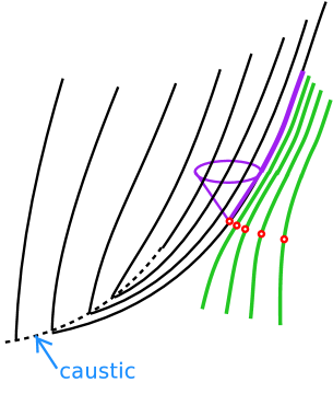
Figure 11: Sketch (in plot of time against space) of segment of black hole horizon showing how a null generator (obtained as limit of escaping timelike curves) can begin (on a caustic) but can never end towards the future.

After it had become clear that (in the framework of Einstein’s theory) the Kerr solutions (with ${\color[rgb]{0.6,0.2,0.0}a}\leq{\color[rgb]{0.6,0.2,0.0}m}$ ) are the only vacuumm black hole equilibrium states, the next thing to be investigated was the way the black holes will evolve when the equilibrium is perturbed. A particularly noteworthy result, based on concepts (see Figure 11 ) developed in collaboration with Penrose [63] was the demonstration by Stephen Hawking [64, 51] that the area of a black hole horizon (which is proportional to what Christodoulou [65] had previously identified as irreducible mass) can never decrease. More particularly it was shown [66] that the area would grow, not only when the hole swallowed matter but more generally whenever the null generators of the horizon were subjected to shear. It was remarked that this effect could be described in terms of an effective viscosity and that the horizon could also be characterised [67, 68] by an effective resistivity.

Later astrophysical developments were concerned more with surrounding or infalling matter – for example in accretion discs – than with the black hole as such, at least until recently. However the prospect of detecting gravitational radiation in the foreseeable future has encouraged a resurgence of interest in purely gravitational effects, particularly those involved in binary coalescence. The climax of a coalescence is too complicated to be dealt with except by advanced methods of numerical computation, but the quasi stationary preliminary stages are more amenable [69, 70, 71, 72, 73, 74], as also are the final stages of ringdown, which can be analysed in terms of quasi normal modes (and their superpositions in power law tails of the kind first described by Price [14]) which have been the subject of considerable attention, particularly concerning the influence of rotation [75, 76, 77, 78, 79].

Appendix: null geodesics in spherical case.

Although it would be insufficient for the complete Kruskal (black and white hole) extension, in order to cover a purely black hole (Oppenheimer Sneyder type) extension of the Schwarzschild solution, it will suffice to use an outgoing null coordinate patch of the kind introduced for the Kerr metric (4) for which, when ${\color[rgb]{0.6,0.2,0.0}a}=0,$ the metric will be given in terms of $x^{{}_{0}}={\color[rgb]{0.3,0.0,0.8}u},$ $x^{{}_{1}}={\color[rgb]{0,0.6,0.2}r},$ $x^{{}_{2}}={\color[rgb]{0.8,0.2,0}\theta},$ $x^{{}_{3}}={\color[rgb]{0.3,0.0,0.8}\phi},$ , simply by

$${\rm d}s^{2}=-\!\left(1-\!{2{\color[rgb]{0.6,0.2,0.0}m}/{\color[rgb]{0,0.6,0.2}r}}\right){\rm d}{\color[rgb]{0.3,0.0,0.8}u}^{2}+2\,{\rm d}{\color[rgb]{0.3,0.0,0.8}u}\,{\rm d}{\color[rgb]{0,0.6,0.2}r}+{\color[rgb]{0,0.6,0.2}r}^{2}{\rm d}{\color[rgb]{0.8,0.2,0}\theta}^{2}+{\rm sin}^{2}{\color[rgb]{0.8,0.2,0}\theta}\,{\rm d}{\color[rgb]{0.3,0.0,0.8}\phi}^{2}\,.$$ (25)

Within such a system, an observer falling in freely from a large distance with zero energy and angular momentum will have a geodesic trajectory characterised by fixed values of the angle coordinates ${\color[rgb]{0.8,0.2,0}\theta}$ and ${\color[rgb]{0.3,0.0,0.8}\phi}$ and by a radial coordinate ${\color[rgb]{0,0.6,0.2}r}$ that is given implicitly as a monotonically decreasing function of proper time by (2) and as a monotonically decreasing function of the ignorable coordinate ${\color[rgb]{0.3,0.0,0.8}u}$ by the relation

$$\frac{{\color[rgb]{0.3,0.0,0.8}u}_{0}-{\color[rgb]{0.3,0.0,0.8}u}}{2{\color[rgb]{0.6,0.2,0.0}m}}=\frac{2}{3}\sqrt{\frac{{\color[rgb]{0,0.6,0.2}r}}{2{\color[rgb]{0.6,0.2,0.0}m}}}\left(\frac{{\color[rgb]{0,0.6,0.2}r}}{2{\color[rgb]{0.6,0.2,0.0}m}}+3\right)-\frac{{\color[rgb]{0,0.6,0.2}r}}{2{\color[rgb]{0.6,0.2,0.0}m}}-2\,{\rm ln}\left\{1+\sqrt{\frac{{\color[rgb]{0,0.6,0.2}r}}{2{\color[rgb]{0.6,0.2,0.0}m}}}\right\}\,,$$ (26)

in which ${\color[rgb]{0.3,0.0,0.8}u}_{0}$ is a constant of integration specifying the value of ${\color[rgb]{0.3,0.0,0.8}u}$ for which the trajectory terminates at the singular limit ${\color[rgb]{0,0.6,0.2}r}\rightarrow 0$ . For such a trajectory the (future oriented) timelike unit tangent vector will be given by

$$e_{{}_{(0)}}^{\ {}_{0}}=\left(1+\sqrt{2{\color[rgb]{0.6,0.2,0.0}m}/{\color[rgb]{0,0.6,0.2}r}}\right)^{-1}\,,\hskip 28.45274pte_{{}_{(0)}}^{\ {}_{1}}=-\sqrt{2{\color[rgb]{0.6,0.2,0.0}m}/{\color[rgb]{0,0.6,0.2}r}}\,,$$ (27)

and the tetrad specifying a corresponding local reference frame can be completed in a natural manner by using the associated (outward oriented) orthogonal spacelike unit vector, which will be given by

$$e_{{}_{(1)}}^{\ {}_{0}}=\left(1+\sqrt{2{\color[rgb]{0.6,0.2,0.0}m}/{\color[rgb]{0,0.6,0.2}r}}\right)^{-1}\,,\hskip 28.45274pte_{{}_{(1)}}^{\ {}_{1}}=1\,,$$ (28)

together with two other horizontally oriented unit vectors whose specification will not matter for the present purpose because of the rotation symmetry of the system.

Let us consider the observation of photon that arrives with trajectory deviating by an angle ${\color[rgb]{0.8,0.2,0}\alpha}$ say from the outward radial direction. The first two components of its (null) momentum vector, ${\color[rgb]{0.8,0.4,0.0}p}^{\mu}$ say, will evidently be given in terms of its energy $\tilde{\color[rgb]{0.6,0.2,0.0}{\cal E}}$ with respect to such a frame by

$${\color[rgb]{0.8,0.4,0.0}p}^{\,i}=\tilde{\color[rgb]{0.6,0.2,0.0}{\cal E}}(e_{{}_{(0)}}^{i}+{\rm cos}\,{\color[rgb]{0.8,0.2,0}\alpha}\,e_{{}_{(1)}}^{i})\,,$$ (29)

for $i=0,1$ . This locally observed energy is to be compared with the globally defined photon energy (as calibrated with respect to the asympotic rest frame at large distance) that will be given in terms of the timelike Killing vector with components ${\color[rgb]{0.3,0.0,0.8}k}^{\mu}=\delta_{{}_{0}}^{\mu}$ by

$${\color[rgb]{0.6,0.2,0.0}{\cal E}}=-{\color[rgb]{0.3,0.0,0.8}k}_{\mu}{\color[rgb]{0.8,0.4,0.0}p}^{\mu}=\left(1-\!{2{\color[rgb]{0.6,0.2,0.0}m}/{\color[rgb]{0,0.6,0.2}r}}\right){\color[rgb]{0.8,0.4,0.0}p}^{{}_{0}}-{\color[rgb]{0.8,0.4,0.0}p}^{{}_{1}}\,,$$ (30)

the important feature of the latter being that it is conserved by the affine transport of the momentum vector along the null geodesic photon trajectory to which it is tangent. It can thus be seen that the corresponding locally observed energy $\tilde{\color[rgb]{0.6,0.2,0.0}{\cal E}}$ will be related to the globally defined energy constant ${\color[rgb]{0.6,0.2,0.0}{\cal E}}$ by

$${\color[rgb]{0.6,0.2,0.0}{\cal E}}=\tilde{\color[rgb]{0.6,0.2,0.0}{\cal E}}(1+Z)\,,$$ (31)

with the redshift $Z$ given by (3), and that the associated component ratio will be given by

$$\frac{{\color[rgb]{0.8,0.4,0.0}p}^{\,{}_{1}}}{{\color[rgb]{0.8,0.4,0.0}p}^{\,{}_{0}}}=(1+\sqrt{2{\color[rgb]{0.6,0.2,0.0}m}/{\color[rgb]{0,0.6,0.2}r}})\left(\frac{{\rm cos}\,{\color[rgb]{0.8,0.2,0}\alpha}-\sqrt{2{\color[rgb]{0.6,0.2,0.0}m}/{\color[rgb]{0,0.6,0.2}r}}}{{\rm cos}\,{\color[rgb]{0.8,0.2,0}\alpha}+1}\right)\,.$$ (32)

As the (unsurprising) spherical limit of the (still rather mysterious) separability of Kerr’s rotating generalisation, the evolution of the relevant affinely transported momentum components will be given in terms of the energy constant ${\color[rgb]{0.6,0.2,0.0}{\cal E}}$ and the associated squared angular momentum constant ${\color[rgb]{0.6,0.2,0.0}{\cal K}}$  [23] (using a dot for differentiation with respect to the affine parameter) by

$${\color[rgb]{0.8,0.4,0.0}p}^{\,{}_{0}}=\dot{\color[rgb]{0.3,0.0,0.8}u}=\frac{\pm\sqrt{\color[rgb]{0,0.6,0.2}{\cal R}}+{\color[rgb]{0,0.6,0.2}{\cal P}}}{{\color[rgb]{0,0.6,0.2}r}^{2}-2{\color[rgb]{0.6,0.2,0.0}m}{\color[rgb]{0,0.6,0.2}r}}\,,\hskip 28.45274pt{\color[rgb]{0.8,0.4,0.0}p}^{{}_{1}}=\dot{\color[rgb]{0,0.6,0.2}r}=\frac{\pm\sqrt{\color[rgb]{0,0.6,0.2}{\cal R}}}{{\color[rgb]{0,0.6,0.2}r}^{2}}\,,$$ (33)

where

$${\color[rgb]{0,0.6,0.2}{\cal P}}={\color[rgb]{0.6,0.2,0.0}{\cal E}}{\color[rgb]{0,0.6,0.2}r}^{2}\,,\hskip 28.45274pt{\color[rgb]{0,0.6,0.2}{\cal R}}={\color[rgb]{0,0.6,0.2}{\cal P}}^{2}-{\color[rgb]{0.6,0.2,0.0}{\cal K}}({\color[rgb]{0,0.6,0.2}r}^{2}-2{\color[rgb]{0.6,0.2,0.0}m}{\color[rgb]{0,0.6,0.2}r})\,.$$ (34)

We thereby obtain

$$\frac{{\color[rgb]{0.8,0.4,0.0}p}^{\,{}_{0}}}{{\color[rgb]{0.8,0.4,0.0}p}^{\,{}_{1}}}=\frac{{\rm d}{\color[rgb]{0.3,0.0,0.8}u}}{{\rm d}{\color[rgb]{0,0.6,0.2}r}}=(1-2{\color[rgb]{0.6,0.2,0.0}m}/{\color[rgb]{0,0.6,0.2}r})^{-1}\left(1\pm\frac{{\color[rgb]{0,0.6,0.2}{\cal P}}}{\sqrt{{\color[rgb]{0,0.6,0.2}{\cal R}}}}\right)\,,$$ (35)

and hence, by comparison with (32),

$$\pm\frac{\sqrt{{\color[rgb]{0,0.6,0.2}{\cal R}}}}{{\color[rgb]{0,0.6,0.2}{\cal P}}}=\sqrt{{\color[rgb]{0,0.6,0.2}r}/2{\color[rgb]{0.6,0.2,0.0}m}}\left(\frac{{\rm cos}\,{\color[rgb]{0.8,0.2,0}\alpha}-\sqrt{2{\color[rgb]{0.6,0.2,0.0}m}/{\color[rgb]{0,0.6,0.2}r}}}{\sqrt{{\color[rgb]{0,0.6,0.2}r}/2{\color[rgb]{0.6,0.2,0.0}m}}-{\rm cos}\,{\color[rgb]{0.8,0.2,0}\alpha}}\right)\,.$$ (36)

This expression can be used to evaluate the squared angular momentum constant as a function of the locally defined energy $\tilde{\color[rgb]{0.6,0.2,0.0}{\cal E}}$ and angle ${\color[rgb]{0.8,0.2,0}\alpha}$ in the form

$${\color[rgb]{0.6,0.2,0.0}{\cal K}}={\color[rgb]{0,0.6,0.2}r}^{2}\tilde{\color[rgb]{0.6,0.2,0.0}{\cal E}}{{}^{2}}{\rm sin}^{2}{\color[rgb]{0.8,0.2,0}\alpha}$$ (37)

in which the variable $\tilde{\color[rgb]{0.6,0.2,0.0}{\cal E}}$ will itself be given via (31) in terms of the globally defined energy constant ${\color[rgb]{0.6,0.2,0.0}{\cal E}}$ by the – red or blue – shift formula (3) so that for the square of the constant ratio of angular momentum to energy one obtains

$$\frac{{\color[rgb]{0.6,0.2,0.0}{\cal K}}}{{\color[rgb]{0.6,0.2,0.0}{\cal E}}^{2}}=\left(\frac{{\color[rgb]{0,0.6,0.2}r}\,{\rm sin}\,{\color[rgb]{0.8,0.2,0}\alpha}}{1-\sqrt{2{\color[rgb]{0.6,0.2,0.0}m}/{\color[rgb]{0,0.6,0.2}r}}\,{\rm cos}\,{\color[rgb]{0.8,0.2,0}\alpha}}\right)^{2}\,.$$ (38)

With respect to an unconventional affine parameter orientation condition to the effect that the energy should always be non-negative, ${\color[rgb]{0.6,0.2,0.0}{\cal E}}\geq 0\,,$ it can be seen (in view of the consideration that the squared angular momentum constant must necessarily be non-negative, ${\color[rgb]{0.6,0.2,0.0}{\cal K}}\geq 0$ ) that a null geodesic segment will be appropriately be describable as “incoming” or “outgoing” according to whether the upper or lower of the sign possibilities $\pm$ is applicable, i.e. according to whether the right hand side of (36) is positive or strictly negative. It is however to be remarked that this convention will be consistent with the usual requirement that the affine parameter orientation be future oriented, giving $\dot{\color[rgb]{0.3,0.0,0.8}u}\geq 0$ , only outside the horizon and for “ingoing” null segments within the horizon, where ${\color[rgb]{0,0.6,0.2}r}<2{\color[rgb]{0.6,0.2,0.0}m}\,,$ but that for “outgoing” null segments within the horizon it would entail the opposite orientation convention, giving $\dot{\color[rgb]{0.3,0.0,0.8}u}\leq 0$ . With respect to the usual parameter orientation condition giving $\dot{\color[rgb]{0.3,0.0,0.8}u}\geq 0$ the “outgoing” null segments within the horizon will need to be parametrised the other way round, which means that they will be characterised by negative energy ${\color[rgb]{0.6,0.2,0.0}{\cal E}}<0$ and by the upper of the sign possibilities $\pm$ .

Whichever convention is used, it can be seen that within the horizon the radius ${\color[rgb]{0,0.6,0.2}r}$ will aways be a decreasing function of ${\color[rgb]{0.3,0.0,0.8}u}$ , even for the (relatively) “outgoing” null segments, and that only an “incoming” null segment can cross the horizon at a finite value of ${\color[rgb]{0.3,0.0,0.8}u}$ . It can be seen from (36) that outside the horizon (i.e. for ${\color[rgb]{0,0.6,0.2}r}>2{\color[rgb]{0.6,0.2,0.0}m}$ ) the criterion for a null segment to be classified as “incoming” is that it should have ${\rm cos}\,{\color[rgb]{0.8,0.2,0}\alpha}\leq\sqrt{2{\color[rgb]{0.6,0.2,0.0}m}/{\color[rgb]{0,0.6,0.2}r}}$ and that the corresponding requirement within the horizon is ${\rm cos}\,{\color[rgb]{0.8,0.2,0}\alpha}\leq\sqrt{{\color[rgb]{0,0.6,0.2}r}/2{\color[rgb]{0.6,0.2,0.0}m}}\,.$

It can be deduced from the expression (34) that the function ${\color[rgb]{0,0.6,0.2}{\cal R}}$ will remain positive wherever ${\color[rgb]{0,0.6,0.2}r}$ is positive if ${\color[rgb]{0.6,0.2,0.0}{\cal K}}/{\color[rgb]{0.6,0.2,0.0}{\cal E}}^{2}\leq 27{\color[rgb]{0.6,0.2,0.0}m}^{2}$ . In such a case, the null geodesic will either be permanently “incoming”, proceding all the way from “infinity” (i.e. the limit ${\color[rgb]{0,0.6,0.2}r}\rightarrow\infty$ ) down to the internal singularity (i.e. the limit ${\color[rgb]{0,0.6,0.2}r}\rightarrow 0$ ), or else it will be permanently “outgoing”, proceding all the way to the singularity or to infinity depending on whether it inside or outside the finite horizon radius value ${\color[rgb]{0,0.6,0.2}r}=2{\color[rgb]{0.6,0.2,0.0}m}$ to which it extends in the infinite past, i.e. as ${\color[rgb]{0.3,0.0,0.8}u}\rightarrow-\infty$ . As well the such “ingoing” and permanently “outgoing” possibilities, the critical case

$${\color[rgb]{0.6,0.2,0.0}{\cal K}}/{\color[rgb]{0.6,0.2,0.0}{\cal E}}^{2}=27{\color[rgb]{0.6,0.2,0.0}m}^{2}$$ (39)

includes also the exceptional possibility of a marginally outgoing – effectively “trapped” – null trajectory with fixed radius ${\color[rgb]{0,0.6,0.2}r}=3{\color[rgb]{0.6,0.2,0.0}m}\,.$

When the angular momentum exceeds this critical value, i.e. if ${\color[rgb]{0.6,0.2,0.0}{\cal K}}/{\color[rgb]{0.6,0.2,0.0}{\cal E}}^{2}>27{\color[rgb]{0.6,0.2,0.0}m}^{2}\,,$ there will be a forbidden range ${\color[rgb]{0,0.6,0.2}r}_{-}<{\color[rgb]{0,0.6,0.2}r}<{\color[rgb]{0,0.6,0.2}r}_{+}$ of values of ${\color[rgb]{0,0.6,0.2}r}$ for which ${\color[rgb]{0,0.6,0.2}{\cal R}}<0$ . It can be seen from 34 that relevant limits are explicitly obtainable, as the non negative solutions of the cubic equation

$${\color[rgb]{0.6,0.2,0.0}{\cal E}}^{2}{\color[rgb]{0,0.6,0.2}r}_{\pm}^{3}-{\color[rgb]{0.6,0.2,0.0}{\cal K}}({\color[rgb]{0,0.6,0.2}r}_{\pm}-2{\color[rgb]{0.6,0.2,0.0}m})=0\,,$$ (40)

in the form

$${\color[rgb]{0,0.6,0.2}r}_{\pm}=2\sqrt{{{\color[rgb]{0.6,0.2,0.0}{\cal K}}}/{3{\color[rgb]{0.6,0.2,0.0}{\cal E}}^{2}}}\,{\rm cos}\,\{\psi_{\pm}/3\}\,,$$ (41)

with

$$\psi_{\pm}={\pi}\mp\,{\rm arcsin}\sqrt{1-{27{\color[rgb]{0.6,0.2,0.0}{\cal E}}^{2}{\color[rgb]{0.6,0.2,0.0}m}^{2}}/{{\color[rgb]{0.6,0.2,0.0}{\cal K}}}}\,,$$ (42)

which evidently entails the conditions $2{\color[rgb]{0.6,0.2,0.0}m}<{\color[rgb]{0,0.6,0.2}r}_{-}<3{\color[rgb]{0.6,0.2,0.0}m}<{\color[rgb]{0,0.6,0.2}r}_{+}\,.$

This means that for a value of ${\color[rgb]{0.6,0.2,0.0}{\cal K}}/{\color[rgb]{0.6,0.2,0.0}{\cal E}}^{2}$ above the critical bound (39) the possible null trajectories will be classifable as “free” or “trapped”. The “free” geodesics are initially “incoming” from “infinity” but become “outgoing” after reaching the inner bound at ${\color[rgb]{0,0.6,0.2}r}={\color[rgb]{0,0.6,0.2}r}_{+}$ so as to remain in the range ${\color[rgb]{0,0.6,0.2}r}\geq{\color[rgb]{0,0.6,0.2}r}_{+}$ . The “trapped” geodesics are either permanently “ingoing” within the horizon or else are initially “outgoing” from just outside the horizion but become “ingoing” after reaching the outer bound ${\color[rgb]{0,0.6,0.2}r}={\color[rgb]{0,0.6,0.2}r}_{-}$ so as to remain within the range ${\color[rgb]{0,0.6,0.2}r}\leq{\color[rgb]{0,0.6,0.2}r}_{-}$ .

For a position in the range ${\color[rgb]{0,0.6,0.2}r}\leq 3{\color[rgb]{0.6,0.2,0.0}m}$ the only kinds of “bright” geodesic, meaning those coming from the distant sky at “infinity”, are of the permanently “incoming” kind characterised by ${\color[rgb]{0.6,0.2,0.0}{\cal K}}/{\color[rgb]{0.6,0.2,0.0}{\cal E}}^{2}\leq 27{\color[rgb]{0.6,0.2,0.0}m}^{2}\,.$ whereas for a position in the range ${\color[rgb]{0,0.6,0.2}r}\leq 3{\color[rgb]{0.6,0.2,0.0}m}$ there will also be “bright” geodesics of the “free” kind characterised by ${\color[rgb]{0.6,0.2,0.0}{\cal K}}/{\color[rgb]{0.6,0.2,0.0}{\cal E}}^{2}>27{\color[rgb]{0.6,0.2,0.0}m}^{2}\,.$ Apart from the special case of the circular null geodesics at ${\color[rgb]{0,0.6,0.2}r}=3{\color[rgb]{0.6,0.2,0.0}m}\,,$ all the other kinds of null geodesic can be classified as “dark” since they can be seen to have emerged from near the horizon limit radius ${\color[rgb]{0,0.6,0.2}r}\rightarrow 2{\color[rgb]{0.6,0.2,0.0}m}$ in the distant past (the limit ${\color[rgb]{0.3,0.0,0.8}u}\rightarrow-\infty)$ and so can be interpreted as trajectories of very highly redshifted radiation from the infalling matter that be presumed to originally formed the black hole whose static final state is under consideration here.

It can be seen that the ratio ${\color[rgb]{0.6,0.2,0.0}{\cal K}}/{\color[rgb]{0.6,0.2,0.0}{\cal E}}^{2}$ specified as a function of ${\rm cos}\,{\color[rgb]{0.8,0.2,0}\alpha}$ by (38) will be monotonically increasing in the “incoming” range, i.e. for $-1\leq{\rm cos}\,{\color[rgb]{0.8,0.2,0}\alpha}<\sqrt{2{\color[rgb]{0.6,0.2,0.0}m}/{\color[rgb]{0,0.6,0.2}r}}$ where ${\color[rgb]{0,0.6,0.2}r}>2{\color[rgb]{0.6,0.2,0.0}m}$ and for $-1\leq{\rm cos}\,{\color[rgb]{0.8,0.2,0}\alpha}<\sqrt{{\color[rgb]{0,0.6,0.2}r}/2{\color[rgb]{0.6,0.2,0.0}m}}$ where ${\color[rgb]{0,0.6,0.2}r}<2{\color[rgb]{0.6,0.2,0.0}m}$ . At the upper end of this “incoming” range the ratio ${\color[rgb]{0.6,0.2,0.0}{\cal K}}/{\color[rgb]{0.6,0.2,0.0}{\cal E}}^{2}$ the tends to a maximum that will be finite – with value ${\color[rgb]{0,0.6,0.2}r}^{3}/({\color[rgb]{0,0.6,0.2}r}-2{\color[rgb]{0.6,0.2,0.0}m})$ – outside the horizon, but that will be infinite inside the black hole. The ratio ${\color[rgb]{0.6,0.2,0.0}{\cal K}}/{\color[rgb]{0.6,0.2,0.0}{\cal E}}^{2}$ will then decrease monotonically for the higher “outgoing” part of the range of ${\rm cos}\,{\color[rgb]{0.8,0.2,0}\alpha}\,.$

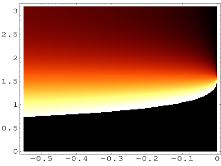
Figure 12: As in Figure 7 but with higher time resolution, showing just final stages after observer passes horizon at ${\color[rgb]{0,0.6,0.2}r}=2{\color[rgb]{0.6,0.2,0.0}m}$ (which occurs when $\tau=-(2/3)^{3/2}\simeq 0.54$ in units used here) as the black hole’s apparent angular radius ${\color[rgb]{0.8,0.2,0}\beta}$ increases towards its upper limit $\pi/2$ when ${\color[rgb]{0,0.6,0.2}r}\rightarrow 0$ .

The critical value (39) will be attained for two values of ${\rm cos}\,{\color[rgb]{0.8,0.2,0}\alpha}\,,$ of which the lower one, ${\rm cos}\,{\color[rgb]{0.8,0.2,0}\alpha}={\color[rgb]{0.8,0.2,0}{\cal X}}_{{}_{-}}$ say, will be in the “incoming” range, and the higher one, ${\rm cos}\,{\color[rgb]{0.8,0.2,0}\alpha}={\color[rgb]{0.8,0.2,0}{\cal X}}_{{}_{+}}$ will be in the “outgoing” range. It can be seen from (38) that these values will be obtainable as the upper and lower roots of

$${\color[rgb]{0,0.6,0.2}r}^{2}(1-{\color[rgb]{0.8,0.2,0}{\cal X}}_{{}_{\pm}}^{\,2})=27{\color[rgb]{0.6,0.2,0.0}m}^{2}(1-\sqrt{2{\color[rgb]{0.6,0.2,0.0}m}/{\color[rgb]{0,0.6,0.2}r}}\,{\color[rgb]{0.8,0.2,0}{\cal X}}_{{}_{\pm}})^{2}\,,$$ (43)

which will be real and distinct except at ${\color[rgb]{0,0.6,0.2}r}=3{\color[rgb]{0.6,0.2,0.0}m}$ where they will coincide.The range of angles characterising the “bright” geodesics will therefore be given by

$$-1\leq{\rm cos}\,{\color[rgb]{0.8,0.2,0}\alpha}<{\rm cos}\,{\color[rgb]{0.8,0.2,0}\beta}$$ (44)

(so that ${\color[rgb]{0.8,0.2,0}\beta}$ will be interpretable as the apparent angular radius of the black hole) with a bounding value ${\rm cos}\,{\color[rgb]{0.8,0.2,0}\beta}$ that will be given by ${\rm cos}\,{\color[rgb]{0.8,0.2,0}\beta}={\color[rgb]{0.8,0.2,0}{\cal X}}_{{}_{-}}\,,$ within the radius of the circular null trajectory, i.e. for ${\color[rgb]{0,0.6,0.2}r}<3{\color[rgb]{0.6,0.2,0.0}m}\,,$ while in the outer regions for which ${\color[rgb]{0,0.6,0.2}r}>3{\color[rgb]{0.6,0.2,0.0}m}$ it will be given by ${\rm cos}\,{\color[rgb]{0.8,0.2,0}\beta}={\color[rgb]{0.8,0.2,0}{\cal X}}_{{}_{+}}\,.$

The required solutions of (43) are expressible in terms of the dimensionless variable $\bar{\color[rgb]{0,0.6,0.2}r}={\color[rgb]{0,0.6,0.2}r}/2{\color[rgb]{0.6,0.2,0.0}m}$ by ${\color[rgb]{0.8,0.2,0}{\cal X}}_{{}_{\pm}}=\left(27\sqrt{\bar{\color[rgb]{0,0.6,0.2}r}}\pm|2\bar{\color[rgb]{0,0.6,0.2}r}^{2}-3\bar{\color[rgb]{0,0.6,0.2}r}|\sqrt{\bar{\color[rgb]{0,0.6,0.2}r}^{2}+3\bar{\color[rgb]{0,0.6,0.2}r}}\right)/(4\bar{\color[rgb]{0,0.6,0.2}r}^{3}+27).$ It can thus be seen that (for the freely falling observer) the apparent angular size ${\color[rgb]{0.8,0.2,0}\beta}$ of the black hole – as shown in the simulation of Figure 1, and as plotted against the proper time (2) in Figure 7 and Figure 12 – will be given as a function of the dimensionless radial variable $\bar{\color[rgb]{0,0.6,0.2}r}={\color[rgb]{0,0.6,0.2}r}/2{\color[rgb]{0.6,0.2,0.0}m}$ by the analytic formula

$${\rm cos}\,{\color[rgb]{0.8,0.2,0}\beta}=\frac{27\sqrt{\bar{\color[rgb]{0,0.6,0.2}r}}+(2\bar{\color[rgb]{0,0.6,0.2}r}^{2}-3\bar{\color[rgb]{0,0.6,0.2}r})\sqrt{\bar{\color[rgb]{0,0.6,0.2}r}^{2}+3\bar{\color[rgb]{0,0.6,0.2}r}}}{4\bar{\color[rgb]{0,0.6,0.2}r}^{3}+27}\,.$$ (45)

.

References

- [1] K.S. Thorne, Black holes and time warps, Einstein’s outrageous legacy, (Norton, New York, 1994).
- [2] J.R. Oppenheimer, H. Snyder, “On continued gravitational contraction”, Phys. Rev. 56 (1939) 455-459.
- [3] T. Regge, J.A. Wheeler, “Stability of a Schwarzschild singularity”, Phys. Rev. 108 (1957) 1063-1069.
- [4] I.D. Novikov, Ya.B. Zel’dovich, “Physics of Rlativistic collapse”, Nuovo Cimento, Supp. bf 4 (1966) 810, Add. 2.
- [5] W. Israel, “Dark stars: the evolution of an idea”, in 300 years of gravitation, ed S.W. Hawking, W. Israel (Cambridge U.P., 1987) 199-276.
- [6] M.D. Kruskal, “Minimal extension of the Schwarzschild metric” Phys. Rev. 119 (1960) 1743.
- [7] W. Israel, “Event horizons in static vacuum spacetimes”, Phys.Rev 164 (1967) 1776-79.
- [8] J.M. Bardeen, “Rapidly rotating stars, disks, and black holes”, in Black Holes (Les Hoches72) ed. B. and C. DeWitt (Gordon and Breach, New York, 1973) 241-289.
- [9] I.D. Novikov, K.S. Thorne,, “Astrophysics of black holes”, in Black Holes (Les Hoches72) ed. B. and C. DeWitt (Gordon and Breach, New York, 1973) 343-450.
- [10] D.N. Page, K.S. Thorne, “Disk accretion onto a black hole. I Time averaged structure of accretion disk”, Astroph. J. 191 (1974) 499-506.
- [11] J.P. Luminet, “Image of a spherical black hole with thin accretion disk”, Astron. Astroph. 75 (1979) 228-235.
- [12] J.A. Marck, “Short cut method of solution of geodesic equations for Schwarzschild black hole”, Class. Quantum Grav. 13 (1996) 393-402. [gr-qc/9505010]
- [13] C.V. Vishveshwara, “Stability of the Schwarschild metric”, Phys. Rev. D1 (1970) 2870-2879.
- [14] R.H. Price, “Nonspherical perturbations of relativistic gravitational collapse”, Phys. Rev. D5 (1972) 2419-2454.
- [15] R. Penrose, “Gravitational collapse and spacetime singularities”, Phys. Rev. Lett. 14 (1965) 57-59.
- [16] R. Penrose, “Gravitational collapse: the role of general relativity”, Nuovo Cimento 1 (1969) 252-276.
- [17] R. Kerr, “Gravitational field of a spinning mass as an example of algebraically special metrics”, Phys. rev. Let. 11 (1963) 237-238.
- [18] R.P. Kerr and A. Schild, “Some algebraically degenerate solutions of Einstein’s gravitational field equations”, Proc. Symp. Appl. Math. 17, (1965) 199.
- [19] R.H. Boyer, T.G. Price, “An interpretation of the Kerr metric in General Relativity”, Proc. Camb.Phil.Soc. 61 (1965) 531-34.
- [20] R.H. Boyer, “Geodesic orbits and bifurcate Killing horizons”, Proc. Roy. Soc. Lond A311, 245-52 (1969).
- [21] B. Carter, “Complete Analytic Extension of Symmetry Axis of Kerr’s Solution of Einstein’s Equations”, Phys. Rev. 141 (1966), 1242-1247.
- [22] R.H. Boyer, R.W. Lindquist, “Maximal analytic extension of the Kerr metric”, J. Math. Phys. 8 (1967) 265-81.
- [23] B. Carter, “Global Structure of the Kerr Family of Gravitational Fields”,Phys. Rev. 174 (1968) 1559-71.
- [24] B. Carter, “Black hole equilibrium states”, in Black Holes (1972 Les Houches Lectures), eds. B.S. DeWitt and C. DeWitt (Gordon and Breach, New York, 1973) 57-210.
- [25] B. Carter, “Domains of Stationary Communications in Space-Time”, B. Carter, Gen. Rel. and Grav. 9, pp 437-450 (1978).
- [26] B. Whiting, “Mode stability of the Kerr blackhole”, J. Math. Phys. 30 (1989) 1301-05.
- [27] M. Simpson, R. Penrose, Int. J. Th. Phys. 7 (173) 183.
- [28] S. Chandrasekha, J.B. Hartle, Proc R. Soc. Lond. A284 (1982) 301.
- [29] E. Poisson, W. Israel, “Internal structure of black holes”, Phys. Rev. D41 (1990) 1796-1809.
- [30] A. Ori, “Structure of the singularity inside a realistic rotating black hole” Phys. Rev. Lett 68 (1992) 2117-2120.
- [31] A. Ori, E.E. Flanaghan, “How generic are null spacetime singularities?” Phys. Rev. D53 (1996) 1754-1758. [gr-qc/9508066]
- [32] A. Ori, “A class of time-machine solutions with compact vacuum core”, Phys. Rev. Lett. 95 (2005) 021101. [gr-qc/0503077]
- [33] R.C. Myers and M.J. Perry, “Black holes in higher dimensional space-times”, Ann. Phys. 172 (1986) 304.
- [34] G.W. Gibbons, S.W. Hawking “Cosmological event horizons, thermodynamics, and particle creation”, Phys.Rev. D15 (1977) 2738-2751.
- [35] S.W. Hawking, C.J. Hunter and M.M. Taylor-Robinson, “Rotation and the AdS/CFT correspondence”, Phys. Rev. D59 (1999) 064005. [hep-th/9811056]
- [36] G.W. Gibbons, H. Lu, D.N. Page, C.N. Pope, “Rotating Black Holes in Higher Dimensions with a Cosmological Constant”, Phys. Rev. Lett. 93 (2004) 171102. [hep-th/0409155]
- [37] A. Papapetrou, “Champs gravitationnels stationnaires à symmetrie axiale”, Ann. Inst. H. Poincaré 4 (1986) 83-85.
- [38] B. Carter, “Hamilton-Jacobi and Schrodinger Separable Solutions of Einstein’s Equations”,Commun. Math. Phys. 10 (1968) 280-310.
- [39] R. Penrose, “Naked Singularities”, Ann. N.Y. Acad. Sci. 224 (1973) 125-134
- [40] B. Carter, “Killing Tensor Quantum Numbers and Conserved Quantities in Curved Space”, Phys. Rev. D16 (1977) 3395-3414.
- [41] W. Unruh, “Separability of the neutrino equation in a Kerr background”, Phys. Rev. Lett. 31 (1973) 1265-1267.
- [42] S. Chandrasekhar, “The solution of Dirac’s equation in Kerr geometry” Proc. Ror. Soc. Lond. A349 (1976) 571-575.
- [43] D. Page, “Dirac equation around a charged rotating black hole”, Phys. Rev. D14 (1976) 1509-1510.
- [44] B. Carter, R.G. McLenaghan, “Generalised Total Angular Momentum Operator for the Dirac Equation in Curved Space-Time”, Phys. Rev. D19 (1979) 1093-1097.
- [45] S.A. Teukolsky, “Perturbations of a rotating black hole, I: Fundamental equations for gravitational and electromagnetic perturbations ”, Astroph. J. 185 (1973) 635-47.
- [46] W.H. Press, S.A. Teukolsky, “Perturbations of a rotating black hole, II: Dynamical stability of the Kerr metric ”, Astroph. J. 185 (1973) 649-73.
- [47] E. Newman, E. Couch, K. Chinnapared, A. Exton, A. Prakash, R. Torrence, “Metric of a rotating charged mass”, J. Math. Phys. 6 (1965) 918-919.
- [48] C. Reina, A. Treves, “Gyromagnetic ratio of Einstein-Maxwell fields”, Phys. Rev. D11 (1975) 3031-3032.
- [49] B. Carter, “An Axisymmetric Black Hole has only Two Degrees of Freedom”, B. Carter, Phys. Rev. Letters 26 (1971) 331-33.
- [50] B. Carter, “Mechanics and equilibrium geometry of black holes, membranes, and strings”, in Black Hole Physics, (NATO ASI C364) ed. V. de Sabbata, Z. Zhang (Kluwer, Dordrecht, 1992) 283-357. [hep-th/0411259]
- [51] S.W. Hawking “Black holes in General Relativity”, Commun. Math. Phys. 25 (1972) 152-56.
- [52] D.C. Robinson, “Uniqueness of the Kerr black hole”, Phys, Rev. Lett.34 (1975) 905-06.
- [53] D. Sudarsky, R.M. Wald, “Mass formulas for stationary Einstein-Yang-Mills black holes and a simple proof of two staticity theorems”, Phys. Rev. D47 (1993) 5209-13. [gr-qc/9305023]
- [54] P.T Chrusciel, R.M. Wald, “Maximal hypersurfaces in stationary asymptotically flat spacetimes”, Comm. Math. Phys. 163 (1994) 561-604. [gr-qc/9304009]
- [55] P.T. Chrusciel, R.M. Wald, “On the topology of stationary black holes”, Class. Quantum Grav. 11 (1994) L147-52 . [gr-qc/9410004]
- [56] B. Carter, “Has the black hole equilibrium problem been solved?” in General Relativity, Gravitation, and Relativistic Field Theories, ed. T. Piran (World Scientific, Singapore, 1999) 136-165. [gr-qc/9712 028]
- [57] F.J. Ernst, “New formulation of the axially symmetric gravitational field problem”, Phys. Rev. 167 (1968) 1175-1178.
- [58] D.C. Robinson, “Classification of black holes with electromagnetic fields”, Phys, Rev. D10 (1974) 458-60.
- [59] P.O. Mazur, “Proof of uniqueness of the Kerr-Newman black hole solution”, J. Phys. A15 (1982) 3173-80.
- [60] P.O. Mazur, “Black hole uniqueness from a hidden symmetry of Einstein’s gravity”, Gen. Rel Grav. 16 (1984) 211-15.
- [61] G. Bunting, “Proof of the Uniqueness Conjecture for Black Holes,”(Ph.D. Thesis, Univ. New England, Armadale N.S.W., 1983).
- [62] B. Carter, “The Bunting Identity and Mazur Identity for non-linear Elliptic Systems including the Black Hole Equilibrium Problem”, Commun. Math. Phys. 99 (1985) 563-91.
- [63] S.W. Hawking, R. Penrose, “The singularities of gravitational collapse and cosmology”, Proc. R. Soc. Lond. A314 (1969) 529-528.
- [64] S.W. Hawking “Gravitational radiation from colliding black holes”, Phys. Rev. Lett. 26 (1971) 1344-1346.
- [65] D. Christodoulou, “Reversible and irreversible transformations in black hole physics”, Phys. Rev. Lett. 25 (1970) 1596-1597.
- [66] S.W. Hawking, J.B. Hartle, “Energy and angular momentum flow into a black hole”, Commun. Math. Phys. —bf 27 (1972) 283-290.
- [67] T. Damour, “Black hole eddy currents”, Phys. Rev. D18 (1978) 3598-3604.
- [68] R.L. Znajek, “Charged current loops around Kerr holes”, Mon. Not. R. Ast. Soc. 182 (1978) 639-646.
- [69] A.D. Kulkarney, L.C. Shepley, J.W. York, “Initial data for black holes”, Phys. Lett. A96 (1983) 228-230.
- [70] P. Marronetti, R.A. Matzner, “Solving the initial value problem of two black holes”, Phys. Rev. Lett. 85 (2000) 5500-5503.
- [71] G.B. Cook, “Initial data for binary black hole collisions”, Phys. Rev. D44 (1991) 2983-3000.
- [72] H.P. Pfeiffer, S.A. Teukolsky, G.B. Cook, “Quasi-circular Orbits for Spinning Binary Black Holes”, Phys. Rev. D62 (2000) 104018.
- [73] P. Grandclément, E. Gourgoulhon, S. Bonazzola, “Binary black holes in circular orbits.” Phys. Rev. D65 (2002) 044020, 044021. [gr-qc/0106016]
- [74] G.B. Cook, “Corotating and irrotational binary black holes in quasicircular orbits”, Phys. Rev. D65 (2002) 084003. [gr-qc/0108076]
- [75] E.W. Leaver, “An analytic representation for the quasi-normal modes of Kerr black holes”, Proc. R. Soc. Lond. A402 (1985) 285-298.
- [76] E. Seidel, S. Iyer, “Black hole normal modes: A WKB approach. IV Kerr black holes”, Phys. Rev. D41 (1990) 374-382.
- [77] K.D. Kokkotas, “Normal modes of the Kerr black hole”, Class. Quantum Grav. 8 (1991) 2217-2224.
- [78] H. Onozawa, “Detailed study of quasinormal frequencies of the Kerr black hole”, Phys. Rev. D55 (1997) 3593-3602. [gr-qc/9610048].
- [79] W. Krivan, P. Laguna, P. Papadopoulos, N. Andersson, “Dynamics of perturbations of rotating black holes”, Phys. Rev. D56 (1997) 3395-3404.