A template bank to search for gravitational waves from inspiralling compact binaries I: physical models

Abstract

Gravitational waves from coalescing compact binaries are searched using the matched filtering technique. As the model waveform depends on a number of parameters, it is necessary to filter the data through a template bank covering the astrophysically interesting region of the parameter space. The choice of templates is defined by the maximum allowed drop in signal-to-noise ratio due to the discreteness of the template bank. In this paper we describe the template-bank algorithm that was used in the analysis of data from the Laser Interferometer Gravitational Wave Observatory (LIGO) and GEO 600 detectors to search for signals from binaries consisting of non-spinning compact objects. Using Monte-Carlo simulations, we study the efficiency of the bank and show that its performance is satisfactory for the design sensitivity curves of ground-based interferometric gravitational wave detectors GEO 600, initial LIGO, advanced LIGO and Virgo. The bank is efficient to search for various compact binaries such as binary primordial black holes, binary neutron stars, binary black holes, as well as a mixed binary consisting of a non-spinning black hole and a neutron star.

I Introduction

Long baseline interferometric gravitational wave detectors are either already taking sensitive data (LIGO LIGO , GEO 600 GEO600 and TAMA TAMA ) or will be ready to do so in the near future (Virgo VIRGO ). The most promising candidates for these detectors are coalescing binaries consisting of compact objects such as neutron stars (NS) and/or black holes (BH) in close orbit, losing energy and angular momentum through the emission of gravitational radiation.

In the past decade a lot of research has been carried out in modelling the late-time dynamics of compact binaries and the emitted radiation. To this end post-Newtonian (hereafter PN) approximation has been used in which all the relevant physical quantities are expressed as a perturbative series in the parameter $v$ which is a measure of the relative velocity of the two component masses of the binary. The approximation is now available to a rather high order $v^{7}$ in PN theory BDIWW ; BDI95 ; BIWW96 ; BFIJ ; LB ; BDEI04 . These models are definitely accurate enough to serve as faithful templates for matched filtering the radiation from binary neutron stars (hereafter, BNS) and binaries consisting of primordial black holes (hereafter, PBHs) NakamuraEtAl . This is because both BNS and binary PBHs merge outside the sensitive band of current ground-based instruments and strong relativistic effects that come into play at the time of merger but not properly modelled by the PN theory are unimportant for their observation. In the case of binary black holes (BBH), however, PN models are not quite accurate since these systems will be ultra-relativistic ($v\sim 0.2$-$0.4$) when their frequencies enter the band where the detectors are most sensitive and some of the BBH systems would even coalesce at frequencies where the detectors have the best sensitivity. There are now models that go beyond the PN theory to predict the waveform given out by these systems and the different models for the binary dynamics predict significantly different waveforms.

I.1 Signal models used in the search

Current searches for gravitational waves from inspiralling compact binaries employ template waveforms that are based on the adiabatic, non-adiabatic and phenomenological models. The adiabatic waveforms are obtained by using the PN expansions of the conserved energy $E$ and flux $\cal F$ and solving the energy balance equation $dE/dt=-\cal F,$ which in turn leads to an evolution equation for the angular velocity $\omega(t)$ and hence the phasing of gravitational waves $\varphi(t)=(2\pi)^{-1}\int\omega(t)dt.$ An implicit assumption made in writing the energy balance equation is that $E$ does not change (appreciably) over an orbital timescale. There has been significant amount of activity to understand the poor behaviour Poisson ; DIS1 of the PN scheme resulting in new improved models that are based on the use of re-summation methods to accelerate the convergence of the PN expansions. The Padé re-summation method DIS1 uses rational polynomial approximations of the original Taylor expansions to improve the convergence of the PN series. The non-adiabatic models directly integrate the equations of motion (as opposed to using the energy balance equation) and there is no implicit conservation of energy that is used in the orbital dynamics as, for instance, in the effective-one-body (EOB) approach EOB1 ; EOB2 ; EOB3 ; DIS2 . The EOB maps the real two-body conservative dynamics onto an effective one-body problem wherein a test mass moves in an effective background metric.

The PN, Padé and EOB models produce physical waveforms, as opposed to the phenomenological waveforms BCV1 ; phenomenological templates ; Kalogera . The latter waveforms capture the main features of the physical waveforms but use unphysical parameters. Nevertheless the phenomenological waveforms themselves fit very well with both the adiabatic and non-adiabatic models, because the scheme uses greater number of free parameters and the parameters are extended to vary over a wider range than that which is physically allowed.

I.2 Matched filtering and template banks

Generally speaking, since the signal from a coalescing binary can be modelled reasonably well we can employ matched filtering, which is the optimal strategy to search for signals buried in stationary, Gaussian noise. However, real interferometer noise is neither stationary nor Gaussian, and we have to use additional consistency checks, such as the $\chi^{2}$-test Ballen ; Babak , to discriminate true events from broadband transients of instrumental or environmental origin.

The matched filtering performs a phase-coherent correlation of the data with a template which is a copy of the model waveform weighted down by the expected power spectral density of the data. The gravitational wave signal depends on a set of continuous parameters such as the amplitude, the masses $m_{1},\,m_{2},$ and spins of the stars and a fiducial reference time (taken to be either “time-of-arrival” $t_{0}$ or “epoch-of-coalescence” $t_{C}$) and the corresponding orbital phase $\phi_{0}$. The parameters describing the inclination of the binary orbit and the location of the source on the sky are degenerate with other parameters, and are therefore, ignored in the search problem, although they can be deduced once the response of three or more non-co-located detectors to a gravitational wave event is known. The eccentricity may also be ignored, since it is expected to be negligible (due to orbital circularization) by the time the gravitational radiation enters the frequency band (10-1000 Hz) of a ground-based detector. In this paper we will only concentrate on non-spinning systems for which the dimension of the search is restricted to 4 parameters ($m_{1},\,m_{2},$, $t_{C}$ and $\phi_{0}$ ) excluding the additional 8 parameters to be used in a spinning system search (angular momentum of the system and the spin orientation of each object).

Since the parameters of an incoming gravitational wave signal will not be known a priori, the data must be searched with a set of templates, called a template bank, designed to cover the whole parameter space. The distance between the templates in the parameter space is governed by the trade-off between computational power and loss in detection rate due to the discrete nature of the template bank. The spacing should be chosen so that the loss in signal-to-noise ratio due to the mis-match of the template with the signal does not deprecate the detectability of these sources.

We employ a geometrical approach SD91 ; DS92 ; BSD95 ; Owen96 ; OwenSathyaprakash98 in constructing a template bank, namely we define a metric on the parameter space and use local flatness theorem to place templates at equal distances. The template bank could be seen naively as a uniform grid in the parameter space. However, to emphasize that this is not, in general a trivial task, we suggest to consider placing dots on a sphere at equal distances. Placing templates on the parameter space depends upon two crucial things: (i) geometrical properties of the signal manifold, whether it is flat or curved, and (ii) the coordinates chosen for template placement, which could be curvilinear even when the manifold is flat, or “almost flat”. Indeed, we need to choose a “Lorentzian-like” (or close to it) coordinate frame. The second point is similar to the problem of laying a regular grid on the plane using either Cartesian or polar coordinates. The situation is even more complicated because the metric, in general, depends on the waveform model and the PN order one chooses.

I.3 Filtering with physical and phenomenological templates

The different PN models differ significantly from each other in their prediction of the phasing of the waves, making it necessary to search for binary black holes and neutron stars by using not one but all the different families of waveforms currently available. Luckily enough, as we will show in this paper and an accompanying paper BCS2 , it turns out that we can use a single bank for all the different physical waveforms explored thus far. This bank is currently used by the GEO 600 and LIGO detectors to search for BNS, binary PBHs and BBH LIGOS2bns ; LIGOS2bbh ; LIGOS2PBH . The signal from a BNS sweeps through the detector bandwidth and the two neutron stars can even merge outside the sensitive bandwidth of the current ground-based detectors and the waveforms corresponding to different physical models agree reasonably well among each other (with overlaps very close to unity). For higher mass systems, e.g. BBH, the situation changes, the deviation between the various models getting more significant in the sensitive bandwidth of the detectors.

Since for BBH the model waveforms from different families do not agree well with each other, a template bank that employs one PN family of templates will not be efficient to detect signals from another family. One solution is to filter the data through a number of banks with templates based on all the different models. If the reasonable assumption that at least one of the available PN models is close to the true gravitational wave signal bears out then our bank consisting of templates from all the different PN families should be efficient enough in capturing the coalescence events. Unexpectedly, we have found that the bank works well as long as the template and signal are both from the same family meaning a single template bank might suffice to filter the data through different PN families.

Another approach to this problem is to use a single template bank of phenomenological waveforms BCV1 . Buonanno, Chen and Vallisneri have designed phenomenological waveforms that are motivated by the structure of the PN signal in the Fourier domain which, for high mass systems, has good overlaps with all the known models. They are able to do this by (a) introducing (in the case of non-spinning binaries) two more parameters than are necessary in the case of physical waveforms and (b) allowing the parameters to vary over a wider, and in some cases unphysical, range than in the case of physical waveforms. The advantage in using the phenomenological templates is that they have been designed to give a good fit not only to known models but also to waveforms which could be “in between” these models. However, there is also a disadvantage in using these waveforms as they are very poor in estimating the physical parameters of the emitting system. Moreover, using two filters instead of one increases the computational cost and the threshold to be used. It produces more false alarm due to larger size of the corresponding template bank. So we might want to filter the data with candidate events through a bank of physical templates for the sake of parameter estimation.

In a companion paper we shall define and study the efficiency of a phenomenological template bank to capture different physical models of gravitational wave signals using designed and real sensitivity curves of the various interferometers. We have verified that such a template bank performs well with the minimal expected (or higher) efficiency for signals from BBH systems with total mass in the range $6$-$40\,M_{\odot}$ for designed sensitivity. For sensitivity seen during the second Science run of the LIGO interferometers the bank covers the parameter space with good efficiency in the same range of the total mass and a lower frequency cutoff of 40 to 100 Hz.

I.4 Organisation of the paper

In the rest of this paper we will discuss only issues related to the physical template bank where both signals and templates are based on the physical models of the gravitational waveform from an inspiralling binary. In Sec. II and III we briefly review, respectively, the Fourier-domain representation of the signal and the technique of matched filtering in a geometrical language, with the aim of introducing the notation and language used in Section IV to construct a template bank. Section IV constructs a generic template bank to search for binary inspirals from sources with a wide range of masses and applicable to any interferometer. The template bank specifically targets equal mass binaries but it is suitable for binaries with a small mass ratio as long as the precessional effects due to the spin of the larger body are unimportant. Section V discusses the results of Monte-Carlo simulations performed with different design sensitivity curves from a variety of interferometers. Section VI summarizes the main results of this paper and discusses the application of the template bank introduced in this paper to capture other target models to be presented in a separate publication.

II Inspiral signal in the stationary phase approximation

For the purpose of the template bank design it suffices to use a simple model of the signal. We shall use the Fourier representation of the standard PN waveform in the so-called restricted PN approximation. In this approximation, one neglects the PN corrections to the amplitude of the signal while the corrections to the phase are fully taken into account to the highest order possible/available.

Let us begin with the time-domain representation of the waveform. The response of an interferometric gravitational wave detector to arbitrarily polarized waves from an inspiralling binary of total mass $M=m_{1}+m_{2},$ mass ratio $\eta=m_{1}m_{2}/M^{2}$, at a distance $D$ is given by

$$h(t)=\frac{4A\eta M}{D}\left[\pi Mf(t)\right]^{2/3}\cos[\varphi(t)+\varphi_{C}],$$ (1)

where it is assumed that the detector’s motion is unimportant during the time when the signal sweeps across its bandwidth. Here, $f(t)$ is the (invariant) instantaneous frequency of the signal measured by a remote observer, the phase of the signal $\varphi(t)=2\pi\int^{t_{C}}f(t)dt$ is defined so that it is zero when the binary coalesces at time $t=t_{C},$ $\varphi_{C}$ is the phase of the signal at $t_{C}$ and $A$ is a numerical constant whose value depends on the relative orientations of the interferometer and the binary orbit which when averaged over all angles is 2/5 DIS2 .

One can compute the Fourier transform $\tilde{h}(f)$ of the waveform given in Eq. (1) using the stationary phase approximation BDI95 ; BSD95 :

$$\tilde{h}(f) = \frac{AM^{5/6}}{D\pi^{2/3}}\sqrt{\frac{5\eta}{24}}f^{-7/6}\exp\left[i\Psi(f;\,t_{C},\,\varphi_{C},\,\lambda_{k})+i\frac{\pi}{4}\right]$$ (2)

$$\Psi(f) = 2\pi ft_{C}+\varphi_{C}+\sum_{k}\lambda_{k}f^{(k-5)/3}.$$ (3)

The parameters $\varphi_{C}$ and $t_{C}$ are the so-called extrinsic, or kinematic, parameters and they are defined by the relative orientation and position of the source and the detector and a fiducial time-of-coalescence of the binary. Intrinsic parameters $\lambda_{k}$ are the chirp parameters related to the two masses of the binary. At the 2PN order there are four non-zero chirp parameters, $\lambda_{0},\lambda_{2},\lambda_{3},\lambda_{4}$ ($\lambda_{1}=0$ owing to the fact that there is no 0.5PN term in the PN expansion), given by

$$\lambda_{0} = \frac{3}{128\eta(\pi M)^{5/3}},\ \ \lambda_{2}=\frac{5}{96\pi\eta M}\left(\frac{743}{336}+\frac{11}{4}\eta\right),\ \ \lambda_{3}=\frac{-3\pi^{1/3}}{8\eta M^{2/3}},$$

$$\lambda_{4} = \frac{15}{64\eta(\pi M)^{1/3}}\left(\frac{3058673}{1016064}+\frac{5429}{1008}\eta+\frac{617}{144}\eta^{2}\right).$$ (4)

The chirp parameters are all functions of the two mass parameters – the total mass $M$ and the symmetric mass ratio $\eta$. Instead of the masses we can choose any two of the chirp parameters to characterize the signal. The choice $(\lambda_{0},\,\lambda_{3}),$ in particular, is convenient since the masses can be computed explicitly in terms of these two parameters:

$$M=\frac{-\lambda_{3}}{16\pi^{2}\lambda_{0}},\ \ \eta=\frac{3}{4\lambda_{0}}\left(\frac{-2\pi\lambda_{0}}{\lambda_{3}}\right)^{5/3}.$$ (5)

Often, it is convenient to use chirptimes $\tau_{0}$ and $\tau_{3},$ in lieu of chirp parameters $\lambda_{k},$ given by

$$\tau_{0}=\frac{5}{256\pi f_{L}\eta}\left(\pi Mf_{L}\right)^{-5/3},\ \ \tau_{3}=\frac{1}{8f_{L}\eta}\left(\pi Mf_{L}\right)^{-2/3},$$ (6)

where $f_{L}$ is the lower-cutoff frequency at which the generation of the templates starts. The value assigned to $f_{L}$ should be chosen carefully: while a low value increases the size of the template bank a high value decreases the signal-to-noise ratio. Section IV.2 discusses how to optimally determine the lower frequency cutoff. Finally, the chirptimes can also be inverted in terms of the masses Mohanty :

$$M=\frac{5}{32\pi^{2}f_{L}}\frac{\tau_{3}}{\tau_{0}},\ \ \eta=\frac{1}{8\pi f_{L}\tau_{3}}\left(\frac{32\pi\tau_{0}}{5\tau_{3}}\right)^{2/3}.$$ (7)

The correspondence between the two sets of parameters $(m_{1}\,,m_{2})$ and $(\tau_{0},\,\tau_{3})$ is illustrated in Fig. 2

III Matched filtering search for inspirals

A matched filter is an optimal linear filter to detect a signal of known shape in stationary, Gaussian noise. It can be introduced in several ways and here we shall follow the geometrical formalism BSD95 ; Owen96 of signal analysis which is most convenient for the construction of a template bank Owen96 . The geometrical picture is more easily motivated by considering the detector output as a discrete time-series rather than a continuous function. Without loss of generality we shall follow this standard procedure in summarizing the basic results from differential geometric approach to signal analysis but often we shall also write the equivalent formulas obtained in the continuum limit. Although the signal is considered as a discrete series in time, it will be treated as a continuous function of the signal parameters, which we shall denote as $\vartheta^{\mu}.$ The notation and language followed here closely resembles that in Refs.  CutlerAndFlanagan ; Owen96 ; OwenSathyaprakash98 .

III.1 A Geometric approach to signal analysis

The output $x(t)$ of a detector is not recorded continuously; it is sampled discretely, usually at equal intervals $\Delta t,$ chosen so as to obey the sampling theorem (see e.g., Ref. PercivalWaldon ). Thus, the detector output lasting for a time $T$ and sampled at a rate $f_{s}$ ($f_{s}\equiv(\Delta t)^{-1}$) is a time-series consisting of $N$-samples, $N=T/\Delta t.$ The set of all possible detector outputs forms an $N$-dimensional vector space. A gravitational wave signal characterized by a set of $p$ parameters $\vartheta^{\mu},$ $\mu=0,1,\ldots,p-1,$ sampled in a similar way is also an $N$-dimensional vector. However, the set of all signal vectors don’t form a vector space, although they do form a manifold (a $p$-dimensional surface in an $N$-dimensional vector space), with the parameters serving as a coordinate system.

Further structure can be developed on this manifold by defining a metric. It turns out that the statistic of matched filtering naturally leads to the definition of a scalar product between vectors, which can then be used to induce a metric on the signal manifold. We shall now turn to a brief discussion of the matched filtering in geometrical language.

Let $x_{k}=n_{k}+s_{k}$ [$x(t)=n(t)+s(t)$] denote the output of a stationary detector consisting of instrumental and environmental noise background $n_{k}$ [$n(t)$] and a possible deterministic signal $s_{k}$ [$s(t)$]. We treat $n_{k}$ as a random time-series drawn from a large ensemble whose statistical properties are those of the detector noise. We use $\left<n_{k}\right>$ to denote the average over the ensemble and assume that $n_{k}$ is a stationary Gaussian random process with zero mean. In the frequency domain we denote these quantities as : $\tilde{x}_{m}=\tilde{n}_{m}+\tilde{s}_{m}$ [$\tilde{x}(f)=\tilde{n}(f)+\tilde{s}(f)$], where Fourier series $\tilde{s}_{m}$ [$\tilde{s}(f)$] of the time series $s_{k}$ [$s(t)$] is defined by

$$\tilde{s}_{m}=\sum_{k=0}^{N-1}s_{k}e^{-2\pi imk/N},\ \ \ \ \tilde{s}(f)=\int_{-\infty}^{\infty}s(t)e^{-2\pi ift}dt.$$ (8)

Next, let us introduce the Hermitian inner product of vectors. Given vectors $g$ and $h$ their inner product, denoted $(g,h),$ is defined as

$$(g,h)=2\sum_{k=0}^{N-1}\frac{\tilde{g}_{k}^{*}\tilde{h}_{k}+\tilde{g}_{k}\tilde{h}^{*}_{k}}{S_{hk}},\ \ \ \ (g,h)=2\int_{0}^{\infty}\frac{\tilde{g}(f)^{*}\tilde{h}(f)+\tilde{g}(f)\tilde{h}(f)^{*}}{S_{h}(f)}df.$$ (9)

Here “$*$” denotes the complex conjugate and $S_{h}$ is the one-sided noise power spectral density (PSD) given by

$$\left<\tilde{n}_{k}\tilde{n}^{*}_{m}\right>=\frac{1}{2}S_{hk}\delta_{km},\ \ \ \ \left<\tilde{n}(f_{1})\tilde{n}^{*}(f_{2})\right>=\frac{1}{2}S_{h}(f_{1})\delta(f_{1}-f_{2}).$$ (10)

The inner product naturally leads to the concept of the norm $||h||$ of a vector $h:$ $||h||=\sqrt{(h,h)}$. A vector $h$ is said to be normalized if its norm is equal to unity. If the vector $h$ is to begin with not normalized then we can define a vector with unit norm by

$$\hat{h}=\frac{h}{\sqrt{(h,h)}}.$$ (11)

It follows from the theory of hypothesis testing that in order to detect a known signal, but with an unknown set of parameters $\vartheta^{\mu},$ in stationary Gaussian background noise $n$ one must construct the statistic $\xi$ given by

$$\xi=2\sum_{k=0}^{N-1}\frac{\tilde{x}_{k}^{*}\tilde{h}_{k}(\vartheta^{\mu})+\tilde{x}_{k}\tilde{h}^{*}_{k}(\vartheta^{\mu})}{S_{hk}}=\left(x,h(\vartheta^{\mu})\right)$$ (12)

and maximize it over the parameters $\vartheta^{\mu}.$ Here $h$ is the template and $q\equiv h/S_{h}$ is the optimal filter. However, the terms template and optimal filter are often used interchangeably to mean either of $h$ or $q.$ Writing the above equation in terms of $q$ we see that the statistic $\xi$ is the cross-correlation of the detector output with the optimal filter $q$ and not just with the template $h.$ Although at first this seems strange, upon closer inspection one can see why the optimal filter is not just a copy of the signal we are looking for but the signal divided by the noise PSD. The noise PSD weighs the correlation differently at different frequencies, making greater contribution to the region of the spectrum where the sensitivity is larger (i.e., $S_{h}$ is smaller) and smaller contribution where the sensitivity is weaker (i.e., $S_{h}$ is larger).

The signal-to-noise ratio (SNR) $\rho$ is the mean of the statistic $\xi$ divided by the square-root of its variance given by

$$\rho=\frac{\left<\xi\right>}{\sqrt{\left<\xi^{2}\right>-\left<\xi\right>^{2}}}=\frac{\left<(x,h)\right>}{\sqrt{\left<(x,h)^{2}\right>-\left<(x,h)\right>^{2}}}=\frac{(s,h)}{\sqrt{(h,h)}},$$ (13)

where the last equality follows from Eq. (10) and our assumption that the noise is a stationary random process with zero mean. Thus, the effect of filtering a signal $s$ with a template $h$ is equivalent to projecting the signal $s$ in the direction of $h,$ i.e. $\rho=(s,\hat{h}).$ This projection is, obviously, the greatest when $h=s$ (the matched filter theorem), giving $\rho=\sqrt{(s,s)}.$ When the template is not the same as the signal the SNR is less than the optimal value. That is, in general $\rho\leq\sqrt{(s,s)}.$

III.2 The mis-match metric

We can use the inner product Eq. (9) to induce a metric on the signal manifold. In the rest of this Section we shall assume that our templates are normalized, that is $(h,h)=1.$ The distance between two infinitesimally separated normalized templates on the signal manifold is given by

$$||h(\vartheta^{\mu}+d\vartheta^{\mu})-h(\vartheta^{\mu})||^{2} = \left|\left|h_{\mu}d\vartheta^{\mu}\right|\right|^{2}$$ (14)

$$= \left(h_{\mu},h_{\nu}\right)\,d\vartheta^{\mu}d\vartheta^{\nu}$$

$$\equiv g_{\mu\nu}d\vartheta^{\mu}d\vartheta^{\nu},$$

where $h_{\mu}$ is the partial derivative of the signal $h$ with respect to the parameter $\vartheta^{\mu}$ and Einstein’s convention of summation over repeated indices is assumed. The quadratic form $g_{\mu\nu}\equiv(h_{\mu},\,h_{\nu})$ defines the metric induced on the signal manifold. This metric is the same as the mismatch metric defined in Ref. Owen96 ; OwenSathyaprakash98 . Let $\mathcal{O}(\vartheta^{\mu},\vartheta^{\mu}+\delta\vartheta^{\mu})$ denote the overlap between two infinitesimally separated vectors $h(\vartheta^{\mu})$ and $h(\vartheta^{\mu}+\delta\vartheta^{\mu}),$ that is

$$\mathcal{O}(\vartheta^{\mu},\vartheta^{\mu}+\delta\vartheta^{\mu})\equiv(h(\vartheta^{\mu}+\delta\vartheta^{\mu}),h(\vartheta^{\mu})).$$ (15)

Since our templates are normalized we have $\mathcal{O}(\vartheta^{\mu},\vartheta^{\mu})=1.$ For vectors that are infinitesimally close to each other we can expand the overlap about its maximum value of 1 ($\delta\vartheta^{\mu}\rightarrow 0$):

$$\mathcal{O}(\vartheta^{\mu},\vartheta^{\mu}+d\vartheta^{\mu})=1-\left.M_{\mu\nu}\right|_{\vartheta^{\alpha}}\delta\vartheta^{\mu}\delta\vartheta^{\nu}+\ldots,$$ (16)

where $M_{\mu\nu}=-\frac{1}{2}\frac{\partial^{2}{\cal O}}{\partial\vartheta^{\mu}\partial\vartheta^{\nu}}.$ The mismatch $M$ between the two vectors is $M\equiv 1-\mathcal{O}(\vartheta^{\mu},\vartheta^{\mu}+d\vartheta^{\mu})=g_{\mu\nu}\delta\vartheta^{\mu}\delta\vartheta^{\nu}.$ Thus, the metric on the manifold can be equivalently constructed using either of the following formulas Porter :

$$g_{\mu\nu} = (h_{\mu},h_{\nu})$$ (17)

$$= -\frac{1}{2}\frac{\partial^{2}{\cal O}}{\partial\vartheta^{\mu}\partial\vartheta^{\nu}}.$$ (18)

Next, we introduce the concept of the minimal match $MM$ SD91 ; Owen96 ; OwenSathyaprakash98 . In searching for a signal of known shape but unknown parameters one filters the data through a bank of templates. The templates in the bank are copies of the signal corresponding to a set of values $\vartheta_{i}^{\mu},$ $i=1,2\,\ldots$. The parameters $\vartheta_{i}^{\mu}$ are chosen in such a manner that (a) the bank of templates has at least an overlap of $MM$ with any signal whose parameters are in a given range

$$\min_{\vartheta^{\mu}}\max_{\vartheta^{\mu}_{i}}(h(\vartheta^{\mu}),h(\vartheta^{\mu}_{i}))\geq MM,$$ (19)

and (b) the number of templates is the smallest for the chosen value of $MM.$ The quantity $MM$ is a very important notion in constructing a bank of templates. Indeed, if we assume that the incoming gravitational wave signal $s(\vartheta^{\nu})$ is reproduced exactly by our model, so that $s(\vartheta^{\nu})=A\hat{h}(\vartheta^{\nu})$, then we could have a drop in the SNR due to the coarseness of the template bank. Indeed, if the template nearest to the signal is $\hat{h}(\vartheta^{\nu}_{i})$ then the SNR is given by

$$\rho=\max_{h_{i}}(s,\hat{h_{i}})=A\mathcal{O}(\vartheta^{\mu},\vartheta^{\mu}_{i})\geq A\times MM.$$ (20)

In reality, however, the overlap between the template and the signal can be smaller than the minimal match since our template may not be an accurate representation of the signal. Recall that our templates are based on the solution to a PN expansion of the Einstein’s equations. Thus, our template might not be sufficiently accurate in describing the fully general relativistic gravitational wave signal emitted by a binary during the final stages of the coalescence of two compact objects. A lot of effort in the last 15 years has been focused on improving the PN templates by (a) working out the expansion to higher orders, and (b) employing re-summation techniques that accelerate the convergence of the PN expansion. Current searches for gravitational waves deploy several families of template banks representing the different classes of the signal models. If the signal $s$ and the template $h$ are from different families then an important notion that will be useful in studying the efficiency of the template bank is the so-called fitting factor introduced in Ref. Apostolatos and defined as:

$$FF(s,h(\vartheta^{\mu}_{i}))=\max_{\vartheta^{\mu}_{i}}(\hat{s},\hat{h}(\vartheta^{\mu}_{i}))$$ (21)

The fitting factor incorporates the degree of faithfulness of our templates in detecting the expected signal $s$.

Finally, given the minimal match and the metric on the parameter space one can estimate the number of templates required to cover the desired range of parameters using Owen96

$$N_{b}[g,MM]=\left(2\sqrt{\frac{1-MM}{p}}\right)^{-p}\int\sqrt{|g|}d\vartheta^{\mu},$$ (22)

where $p$ is the number of independent parameters.

Strictly speaking, thequadratic approximation used in Eq. 16 is valid for $\delta\vartheta^{\mu}\rightarrow 0$ Owen96 but for practical purposes the approximation is valid for $MM=90\%-95\%$.

III.3 Application to binary inspirals

Let us now apply the geometrical language of the previous Section to the case of binary inspirals. Our aim is to derive an explicit expression for the metric and then use it to set up a bank of templates. The discussion in the previous Section illustrated the general method for obtaining the metric on a signal manifold whose dimension is equal to the number of parameters characterising the signal. It might at first, therefore, seem as though we would need templates in the full multi-dimensional signal parameter space. We need a bank of templates since we would not know before hand what the parameters of the signal are and have to construct the detection statistic for different possible values of the signal parameters, such that at least one template in our bank is close enough to any possible signal so as not to lose more than, say 5% of the SNR. However, templates are not always explicitly needed to maximize the SNR (as shown by Schutz SchutzInBlair ) in the case of the extrinsic parameters $t_{C}$ and $\varphi_{C},$ thereby greatly reducing the problem of having to filter the data through a large template bank. Indeed, data analysts are always looking for ways to reduce the effective dimensionality of the template space.

The maximization over the phase $\varphi_{C}$ is achieved via the decomposition of the signal into its quadratures: two templates with a $\pi/2$ phase difference, e.g. $\varphi_{C}=0$ and $\varphi_{C}=\pi/2$ SchutzInBlair ; SD91

$$\max_{\varphi_{C}}\rho=\max_{\varphi_{C}}(x,\hat{h}_{i}(\varphi_{C}))=\sqrt{(x,\hat{h}_{i}(0))^{2}+(x,\hat{h}_{i}(\pi/2))^{2}}.$$ (23)

Thus, we need only two templates to search in the $\varphi$-dimension. Similarly, the search for the fiducial time $t_{C}$ at which the binary merges can be efficiently found in practice via the fast Fourier transform

$$\max_{t_{C}}\rho=\max_{t_{C}}\rho(t_{C}),\ \ \ \ \rho(t_{C})=\sum_{m}\frac{\tilde{x}^{*}_{m}\hat{h^{\prime}}_{m}}{S_{hm}}e^{2\pi imt_{C}}.$$ (24)

Thus, we need the metric and the templates only in the two-dimensional space of intrinsic parameters, which are taken to be the chirp parameters $\tau_{0}$ and $\tau_{3}$ instead of the masses $m_{1}$ and $m_{2}$ of the binary. However, it is more convenient to begin with the metric in the three-dimensional space of $(t_{C},\tau_{0},\tau_{3})$ and then project out the coordinate $t_{C}.$

In practice, we can also work with the chirp parameters $\theta_{1}$ and $\theta_{2}$ :

$$\theta_{1}=2\pi f_{L}\tau_{0},\ \ \ \ \theta_{2}=2\pi f_{L}\tau_{3}.$$ (25)

We can use either of Eqs.(17) or (18) to work out the metric. Owen Owen96 used Eq. (18) and maximized the metric over the phase $\varphi_{C}$ to obtain an explicit expression for the metric $\gamma_{\alpha\beta}$ in the three-dimensional space of $(t_{C},\theta_{1},\theta_{2}):$

$$\gamma_{\alpha\beta}=\frac{1}{2}\left(\mathcal{J}[\psi_{\alpha}\psi_{\beta}]-\mathcal{J}[\psi_{\alpha}]\mathcal{J}[\psi_{\beta}]\right),$$ (26)

where $\psi_{\alpha}$ is the derivative of the Fourier phase of the inspiral waveform with respect to the parameter $\theta^{\alpha},$ that is $\psi_{\alpha}\equiv\partial\Psi/\partial\theta_{\alpha},$ and ${\mathcal{J}}$ is the moment functional PoissonAndWill of the noise PSD. For any function $a(x)$ the moment functional $\mathcal{J}$ is defined as,

$$\mathcal{J}[a]\equiv\frac{1}{I(7)}\int^{x_{\rm U}}_{x_{\rm L}}\frac{a(x)\,x^{-7/3}}{S_{h}(x)}\,dx.$$ (27)

where $I(q)$ is the $q$th moment of the noise PSD defined by,

$$I(q)\equiv S_{h}(f_{0})\int^{x_{\rm U}}_{x_{\rm L}}\frac{x^{-q/3}}{S_{h}(x)}\,dx.$$ (28)

Here $x\equiv f/f_{0}$ (also $x_{\rm U}\equiv f_{\rm U}/f_{0}$ and $x_{\rm L}\equiv f_{\rm L}/f_{0}$), $f_{0}$ is a fiducial frequency chosen to control the range of numerical values of the functions entering the integrals, $f_{\rm L}>0$ is the lower-cutoff chosen so that the contribution to the integrals from frequencies smaller than $f_{\rm L}$ is negligible and $f_{\rm U}$ is the upper frequency cutoff corresponding to the system’s last stable orbit frequency. The metric $g_{mk}$ on the subspace of just the masses (equivalently, chirp times) is given by projecting out the coalescence time $t_{C}$:

$$g_{mk}=\gamma_{mk}-\frac{\gamma_{0m}\gamma_{0k}}{\gamma_{00}}.$$ (29)

We shall now derive an explicit formula for the metric on the sub-space of masses by using the chirp parameters $\theta_{1}$ and $\theta_{2}$ from Eq. (25) as our coordinates.

The starting point of our derivation is the Fourier domain phase Eq. (3). By writing the $\lambda_{k}$’s in terms of $\theta_{1}$ and $\theta_{2}$ we get

$$\Psi(f;t_{C},\theta_{1},\theta_{2}) = 2\pi ft_{C}+a_{01}\theta_{1}x^{-5/3}+\left[a_{21}\frac{\theta_{1}}{\theta_{2}}+a_{22}\left(\theta_{1}\theta_{2}^{2}\right)^{1/3}\right]x^{-1}+a_{31}\theta_{2}x^{-2/3}$$ (30)

$$+ \left[a_{41}\frac{\theta_{1}}{\theta_{2}^{2}}+a_{42}\left(\frac{\theta_{1}}{\theta_{2}}\right)^{1/3}+a_{43}\left(\frac{\theta_{2}^{4}}{\theta_{1}}\right)^{1/3}\right]x^{-1/3},$$

where the constants $a_{km}$ are given by:

$$a_{01}=\frac{3}{5},\ \ a_{21}=\frac{11\pi}{12},\ \ a_{22}=\frac{743}{2016}\left(\frac{25}{2\pi^{2}}\right)^{1/3},\ \ a_{31}=-\frac{3}{2},$$

$$a_{41}=\frac{617}{384}\pi^{2},\ \ a_{42}=\frac{5429}{5376}\left(\frac{25\pi}{2}\right)^{1/3},\ \ a_{43}=\frac{15293365}{10838016}\left(\frac{5}{4\pi^{4}}\right)^{1/3}.$$ (31)

The gradients $\psi_{0}=\partial\Psi/\partial t_{C},$ $\psi_{m}=\partial\Psi/\partial\theta_{m}$ enter the moment functionals which can be computed from the foregoing expression for the Fourier phase

$$\psi_{0}=2\pi f,\ \ \ \ \psi_{m}=\sum_{k=0}^{n}\Psi_{mk}x^{(k-5)/3},$$ (32)

where $n$ is the PN order up to which the phase is known, or the PN order at which the metric is desired. Expansion coefficients $\Psi_{mk}$ can be considered to be a $(2\times n)$ matrix, which to 2PN order is given by:

$$\Psi=\left[\begin{matrix}a_{01}&0&{a_{21}}/{\theta_{2}}+({a_{22}}/{3})\left({\theta_{2}}/{\theta_{1}}\right)^{2/3}&0&{a_{41}}/{\theta_{2}^{2}}+{a_{42}}/\left({3\left(\theta_{1}^{2}\theta_{2}\right)^{1/3}}\right)-({a_{43}}/{3})\left({\theta_{2}}/{\theta_{1}}\right)^{4/3}\cr 0&0&-{a_{21}\theta_{1}}/{\theta_{2}^{2}}+(2{a_{22}}/{3})\left({\theta_{1}}/{\theta_{2}}\right)^{1/3}&a_{31}&-{2a_{41}\theta_{1}}/{\theta_{2}^{3}}-({a_{42}}/{3})\left({\theta_{1}}/{\theta_{2}^{4}}\right)^{1/3}+({4a_{43}}/{3})\left({\theta_{2}}/{\theta_{1}}\right)^{1/3}\end{matrix}\right].$$ (33)

It is useful to note that the moment functional of polynomial functions $a(x)=\sum a_{k}x^{k}$ are given by

$$\mathcal{J}\left[\sum_{k}a_{k}x^{k}\right]=\sum_{k}a_{k}J(7-3k),$$ (34)

where $J(q)$ is the normalized moment given by $J(q)=I(q)/I(7).$ Using the definition of the metric in Eq. (26) and projecting out the parameter $t_{C}$, we find

$$g_{ml}=\frac{1}{2}\sum_{k,j=0}^{N}\Psi_{mk}\Psi_{lj}\left\{J(17-k-j)-J(12-k)J(12-j)-\frac{\left[J(9-k)-J(4)J(12-k)\right]\left[J(9-j)-J(4)J(12-j)\right]}{\left[J(1)-J(4)^{2}\right]}\right\}.$$ (35)

IV Template bank based on SPA model

In this Section we will discuss the problem of constructing a bank of templates based on the geometric formalism introduced earlier. To this end we shall use the specific signal model of an inspiral binary discussed in Sec. II. This model uses a restricted PN approximation in which the PN amplitude corrections containing higher order harmonics are neglected. The end result of the construction of the template bank is a set of points in the parameter space of chirptimes or, equivalently, the masses. Each point is associated with a template built from a specific signal model.

In principle, there is nothing in the construction of the bank that forbids us to use as our templates a model that is different from the one discussed in Sec. II. Indeed, we shall show in a companion paper that although we have used a specific signal model in the construction of the bank, the same bank works for a wide variety of other signal models. In this paper we shall mainly focus on the SPA model, and only as an introduction to a more exhaustive study we shall present one case of a physical model based on the time domain Taylor model at 2PN, restricted to the BNS search.

We validate the performance of our template bank and quantify its efficiency (see Sec. V for a precise definition) using Monte Carlo simulations in which a number of signals, with their parameters chosen randomly, are generated and their best overlap with the bank of templates is computed. The algorithm described here is implemented in the LIGO Algorithms Library (LAL) LAL , and currently used by the LIGO Scientific Collaboration (LSC) to search for BNS, BBH and binary PBHs LIGOS2bns ; LIGOS2bbh ; LIGOS2PBH .

IV.1 Effective dimensionality of the parameter space

In order to construct the template bank we will start with the metric defined in Eq. (14). As argued in Sec. III the extrinsic parameters $t_{C}$ and $\varphi_{C}$ do not need to be searched with a template bank. One can analytically maximize the overlap with respect to these parameters locally at each point in the space of masses. Thus, we project $\varphi_{C}$, $t_{C}$ onto the two-dimensional space of masses in which the chirptimes ($\tau_{0},\tau_{3})$ defined by Eq. (6) serve as coordinates. Instead of $(\tau_{0},\tau_{3})$ we can equivalently take any two of the $\tau_{k}$’s to be independent parameters to characterize the signal. The choice ($\tau_{0},\tau_{3}$), is particularly attractive because their relationship to the masses is analytically invertible Mohanty [cf. Eqs. (5) and (6)]. In addition, as we will argue later, the metric in these coordinates is a slowly varying function TanakaTagoshi .

IV.2 Lower frequency cutoff

Before presenting an algorithm to place templates in the parameter space let us discuss how one can choose the lower frequency cutoff $f_{L},$ which essentially determines the size of the parameter space of chirptimes and plays a crucial role in the computational resources required to process the data through the template bank.

The initial fiducial frequency $f_{L}$ defines the range of values of the chirptimes and is not itself a parameter to search for. However, it affects the length of the signals (therefore, the parameter space to be covered) and the SNR extracted. For example, the Newtonian chirptime $\tau_{0}\propto f_{L}^{-8/3};$ thus, lower values of $f_{L}$ give longer templates with the immediate consequence of enhancing both the required storage space for templates and the computational cost to filter the data through the template bank. Furthermore, the number of cycles in a template increases as $N_{\rm cyc}\propto({\cal M}f_{L})^{-5/3},$ affecting both the overlap between different templates and the number of templates in the bank.

What is really important, both for signal recovery and the number of templates required in the bank, is the effective number of cycles DIS2 which depends not only on the lower frequency cutoff but also on the noise PSD of the detector. The reason for this is the following: while the signal power increases with decreasing lower-cutoff as $f_{L}^{-7/3},$ the noise PSD $S_{h}(f)$ increases much faster below a certain frequency determined by the various noise backgrounds. Thus, there will be negligible contribution to the SNR integral and noise moments $J(q)$ from frequencies below a certain lower cutoff. As a consequence, choosing the lower cutoff frequency to be smaller than a certain value has no advantage; on the contrary it has the undesirable effect of increasing the number of templates and the computational cost of the analysis.

The constant minimal match $MM$ has also to be set and we decided to chose a value $MM=95\%$. This value is large enough so that Eq. 16 is still valid and small enough so that the number of templates (Eq. 22) is not too large with respect to computational cost.

Table 1 summarizes the number of templates at a constant minimal match of $MM=95\%$ as a function of $f_{L}$. We can immediately see that for the different PSDs considered, the number of templates evolves significantly as $f_{L}$ is reduced but stabilizes after reaching a certain value. Our aim is to choose the lower frequency cutoff small enough so that it has negligible effect on signal recovery.

Table 1: The number of templates required to search for BNS versus the lower cutoff frequency $f_{L}$ at a minimal match $MM=95\%$. As the cutoff is lowered the number of templates initially increases sharply but stabilizes after reaching a certain value depending on the noise characteristics of the detector in question. The last row gives the lower cutoff frequency that was chosen in our simulations by demanding that the loss in SNR due to this choice is not more than 1%. Note that the number of templates converges at smaller values of $f_{L},$ but we don’t gain in SNR by choosing $f_{L}$ to be that at which the number of templates converge.

f_L(Hz)	GEO 600	LIGO-I	Advanced LIGO	Virgo
$10$	$6085$	$4382$	$18692$	$30650$
$15$	$6099$	$4412$	$12782$	$22068$
$20$	$6113$	$4449$	$9425$	$15992$
$25$	$6129$	$4408$	$7086$	$12027$
$30$	$6145$	$4312$	$5469$	$9140$
$35$	$6002$	$3783$	$4312$	$6958$
$40$	$4914$	$3121$	$3527$	$5504$
$45$	$3768$	$2577$	$2885$	$4358$
$50$	$3017$	$2271$	$2289$	$3458$
Chosen f_L(Hz)	$40$	$40$	$20$	$20$

Choosing the lower frequency cutoff too high leads to a loss in the SNR because, as evident from Eq. (2), there is greater power in the signal at lower frequencies, with the power spectrum of the signal falling with frequency as $f^{-7/3}.$ However, the increase in signal power at lower frequencies does not help beyond a certain point because the SNR integrand is weighted down by the noise PSD of the instrument. Current generation of interferometers are dominated at frequencies below about $30$-$40$ Hz by seismic noise. For instance, in the case of the Virgo interferometer the noise PSD raises as $f^{-4.8}$ at frequencies below about $30\rm Hz$ thereby dictating that setting $f_{L}\sim 30\rm Hz$ might be a reasonable choice.

Essentially, there are two opposing choices for $f_{L}$ and one must make an arbitrary but optimal choice. In this paper, the lower frequency cutoff is chosen as large as possible with the constraint that no more than 1% of the overlap is lost as a result of choosing $f_{L}$ to be different from 0. The choice of $f_{L}$ would then depend, in principle, on the masses of the stars in the binary. This is because the templates are shutoff when the binary reaches the innermost circular orbit, making the bandwidth available to integrate the signal smaller, and forcing to choose a lower cutoff that is smaller for higher masses. However, again because of the steep increase in the seismic noise below a certain frequency, signals from binaries of total mass greater than $\sim 100M_{\odot}$ will not be visible in the first generation instruments.

In Fig. 1 we plot the highest value of lower cutoff as a function of the total mass of the binary by requiring that the loss in the SNR is no more than 1%. The different curves in the plot correspond to the noise PSD expected in various ground-based interferometers. There is no need to make these plots for systems with different mass ratios since, at the level of approximation we are using, the cutoff depends only on the total mass and not on the mass ratio of the system. The left panel plots the lower cutoff frequency, which gives a loss in SNR of 1%, as a function of the total mass when the ending frequency of the system is set at the last stable orbit (LSO). The right panel shows the same result when the upper frequency is set at the light ring (EOB models at 2PN). Our choice of lower frequency cutoff is summarized in Table 1.

There is subtlety OwenPrivate in the choice of the lower-frequency cutoff. The optimal SNR is only sensitive to the lower-frequency cutoff but not the parameters of the template and the signal because they are both assumed to be the same. When filtering the data through a template bank, however, we have no optimal templates but for a set of measure zero signals. Consequently, what is important is not the behaviour of the SNR (which only depends on the moment $J[7]$) but that of the metric (which is sensitive to the difference in the parameter values of neighbouring templates). The metric is highly sensitive to the moment $J[17],$ which converges rather slowly as a function of the lower-cutoff. We have chosen the easier approach described above in choosing the lower-cutoff, as that is less sensitive to the parameters of the system. The real justification comes from the fact that our choice of the lower-cutoff does not seem to have severely affected the efficiency of the template bank as we shall see later in this paper.

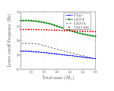
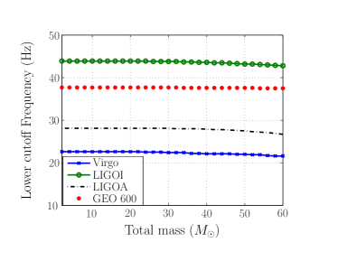
Figure 1: The four curves in each plot show the lower frequency cutoff that corresponds to a loss of SNR of 1%, respectecly for the GEO 600, LIGO-I, Advanced LIGO and Virgo, using the ending frequency of the binary to be the last stable orbit (left panel) and the light ring (right panel).

IV.3 Template placement algorithm

The templates are chosen in the parameter space such it is guaranteed that for every signal in the region of interest there will be at least one template in the bank with an overlap larger than or equal to the minimal match. In addition to the templates within the parameter space of the search a layer of templates might also be required just outside the boundary of the parameter space to assure the chosen minimal match for all signals within the parameter space. This happens because some of the templates that lie outside the boundary have coverage within the parameter space; without them signals with their parameters near the boundary might not have the desired minimal match OwenPrivate .

The template placement algorithm consists of two steps: the first step deals with placing templates along a chosen curve in the parameter space, specifically along the equal-mass curve, while the second step deals with the placement of templates within and outside the boundary of the parameter space.

The preference of chirptimes (or chirp parameters) over masses as coordinates on the signal manifold is dictated by the fact that these variables are almost Cartesian. This is clearly seen when considering the 1PN model for which the metric $g_{\mu\nu}\equiv\left(h_{\mu},\,h_{\nu}\right)$ is a constant, i.e. independent of the chirptimes, while the same metric expressed in $(M,\eta)$ or $(m_{1},m_{2})$ coordinates is not a constant. Thus, the signal manifold at 1PN order is not only flat, the chirptimes are Cartesian-like coordinates. When we go to higher PN orders, the multi-dimensional signal manifold, in which all chirptimes are considered to be independent of one another, is again a flat manifold but the physical chirp manifold (i.e. the manifold formed by signals expected from the inspiral of black hole binaries) is only a two-dimensional manifold that is obtained by imposing the constraints $\tau_{3}=\tau_{3}(\tau_{0},\tau_{1})$, $\tau_{4}=\tau_{4}(\tau_{0},\tau_{1})$, and so on. This physical manifold, could, in principle, be a curved manifold but the curvature is not likely to be large since the absolute value and range of higher order chirptimes is small compared to the most dominant chirptimes. Hence the constraints are unlikely to result in a large curvature. We shall, therefore, assume that the metric is essentially constant in the local vicinity (on the scale defined by mismatch) of every point on the manifold.

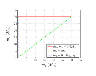
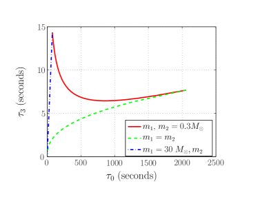
Figure 2: The left panel shows an example of the range of masses covered by the template bank while the right panel shows the corresponding region in the space of chirptimes $\tau_{0}$-$\tau_{3}.$ The shape of the detector’s PSD does not enter in the definition of the chirptimes but the lower frequency cutoff does and is taken to be $f_{L}=20$ Hz. The individual mass range is chosen to be [0.3, 30]$M_{\odot}$ including the BNS, BBH and PBHs binary systems.

In this work we shall specifically choose $(\tau_{0},\,\tau_{3})$ to be the coordinate system. As we also mentioned above, the masses are analytically invertible in terms of this pair of chirptimes [cf. Eq. (5)]. The range of masses accessible to various interferometers is shown in Fig. 2 together with the corresponding space of chirptimes. Note that since $\eta\leq 1/4$ not all of the $M$-$\eta$ or $\tau_{0}$-$\tau_{3}$ space is physically meaningful. In the $M$-$\eta$ space the region above $\eta=1/4$ is forbidden while in the space of $\tau_{0}$-$\tau_{3}$ the region below the curve marked $m_{1}=m_{2}$ is forbidden. As we do not wish to place templates in this forbidden region (although this is, in principle, perfectly possible) the loss in SNR will be more than the minimal match if we do not place templates along the equal-mass curve. Imagine starting from the boundary on the left of the space of chirptimes and placing templates along the $\tau_{3}=\rm const.$ line. Eventually, the algorithm would take us beyond the boundary on the right and a proper coverage of the parameter space would require us to place a template in the forbidden region. Placing this last template on the equal-mass curve is not a solution as this could create a “hole” in the parameter space. For signals in the “hole” the overlap obtained will be less than the minimal match.

Thus, our template placement algorithm consists of two steps: After computing the minimum and maximum chirp-times corresponding to the search space, namely $(\tau_{0}^{\rm min},\tau_{0}^{\rm max})$ and $(\tau_{3}^{\rm min},\tau_{3}^{\rm max}),$ the algorithm chooses a lattice of templates along the equal mass curve, lays a grid of templates in the rectangular region defined by the minimum and maximum values of the chirptimes and rejects the lattice point if the point itself lies outside the parameter space and none of the vertices of the rectangle inscribed within ambiguity ellipse lie within the parameter space.

IV.3.1 Templates along the $\eta=1/4$-curve

In the first stage, templates are built along the equal mass (that is, $\eta=1/4$) curve starting from the minimum value of the Newtonian chirp-time and stopping at its maximum value. The algorithm is illustrated in Fig. 3: given the $n$-th template at $O$ with parameters $(\tau_{0}^{n},\tau_{3}^{n}),$ and the distance $(\delta\tau_{0}^{n},\delta\tau_{3}^{n})$ between templates in our preferred coordinates, consider lines $\tau_{0}=\tau_{0}^{n}+\delta\tau_{0}^{n}$ ($QA$ in Fig. 3) and $\tau_{3}=\tau_{3}^{n}+\delta\tau_{3}^{n}$ ($PB$ in Fig. 3). The template next to $(\tau_{0}^{n},\tau_{3}^{n}),$ on the equal mass curve, must lie either along $PB$ or along $QA$ (cf. Fig. 3) in order that all the signals that may lie on $OAB$ are spanned by at least one of the two templates. Clearly, if we were to place the $(n+1)$-th template at $B$ there will be a gap and some of the signals will not have the required minimal match; placing it at $A$ meets our requirement.

Note, however, that there is no guarantee that this will always work; it would indeed fail if the curve along which templates are being laid is a rapidly varying function. However, there is no danger of this happening in the case of the $\eta=1/4$ curve. Indeed, for increments $\delta\tau_{0}$ equal to the distance between templates expected at a minimal match of 0.95 we can assume the curve to be a straight line: $\tau_{3}\approx\tau_{3}^{0}+\dot{\tau}_{3}^{0}\delta\tau_{0},$ where $\dot{\tau}_{3}$ is the derivative with respect to $\tau_{0}$ along the $\eta=1/4$ curve. Therefore, the above algorithm will never fail in our case.

To locate the $(n+1)$-th template we compute the following pairs of chirptimes:

$$\tau_{0}^{n+1}=\tau_{0}^{n}+\delta\tau_{0}^{n},\ \ \tau_{3}^{n+1}=4A_{3}\left(\frac{\tau_{0}^{n+1}}{4A_{0}}\right)^{2/5}$$

$$\tau_{3}^{n+1}=\tau_{3}^{n}+\delta\tau_{3}^{n},\ \ \tau_{0}^{n+1}=4A_{0}\left(\frac{\tau_{3}^{n+1}}{4A_{3}}\right)^{5/2},$$ (36)

where

$$A_{0}=\frac{5}{256(\pi f_{L})^{8/3}},\ \ A_{3}=\frac{\pi}{8(\pi f_{L})^{5/3}}.$$ (37)

Of the two pairs, the required pair is the one that is closer to the starting point $(\tau_{0}^{n},\tau_{3}^{n}).$

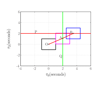
Figure 3: Algorithm sketching the placement of templates along the $\eta=1/4$ curve. The placement uses the rectangle inscribed in the ambiguity ellipse around each point of the parameter space considered.

IV.3.2 Templates in the rest of the parameter space

In the second stage, the algorithm begins again at the point $(\tau_{0}^{\rm min},\tau_{3}^{\rm min}),$ with the corresponding distance between templates $(\delta\tau_{0}^{\rm min},\delta\tau_{3}^{\rm min}),$ and chooses a rectangular lattice of templates in the region defined by $(\tau_{0}^{\rm min},\tau_{3}^{\rm min})$ $(\tau_{0}^{\rm max},\tau_{3}^{\rm min})$ $(\tau_{0}^{\rm max},\tau_{3}^{\rm max})$ and $(\tau_{0}^{\rm min},\tau_{3}^{\rm max})$. A template is accepted either if its coordinate is within the parameter space of search or if its span, for the given minimal match, has an overlap with the parameter space. It is this latter requirement that allows for a layer of templates just outside the boundary of the parameter space. These templates will have overlaps larger than or equal to $MM$ for some signals within the parameter space of interest; leaving them out would cause ‘holes’ in the template bank where the match achieved by the template bank will be smaller than the minimal match.

The implementation of the algorithm along the equal mass curve and in a rectangular lattice in the rest of the parameter space is plotted in Fig. 4 where the chosen templates are represented as points and the ellipses around the points. The ellipses define the regions where the overlap is greater than or equal to the minimal match. A sketch of the implementation of the algorithm is given in Appendix References for both the placement along the equal mass curve and the rest of the parameter space.

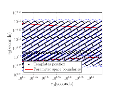
Figure 4: Algorithm sketching the construction of a rectangular lattice of templates. Using the placement algorithm as shown in Fig. 3, the parameter space can be spanned with ellipses using their inscribed rectangles.

In summary, the following parameters are required to compute the grid in the parameter space:

• minimum mass of the component stars,

• maximum total mass of the binary system,

• minimal match which defines the distance between the nearby templates in the parameter space,

• noise power spectral density $S_{h}(f)$ of the detector in question,

• lower and upper frequency cutoffs used in computing the moments of the noise PSD.

V Validation of the template bank

We have carried out Monte-Carlo simulations to study the efficiency of the template bank described in the previous Section. By efficiency we mean the ability of the bank to capture signals with the loss in SNR no more than the one defined by $MM$, the minimal match. The Monte-Carlo simulations consist in generating a number $N_{s}$ of random normalised signals $\hat{s}$ and finding the fitting factor $FF$ between the signal and the bank of templates. We use $\hat{s}$ to denote the signal in order to distinguish it from the template $\hat{h}$ used in the bank. The models used to generate $\hat{s}$ and $\hat{h}$ are based on the SPA model at 2PN described in the Section II. We randomize the parameters ($m_{1},m_{2}$) in the range covered by the template bank as well as the initial phase $\varphi_{C}$. Another issue is the randomization of the mass parameters, for which there are several choices: one choice could be to have a uniform distribution of component masses. However, this choice will not probe our template bank properly; indeed, the corresponding distribution of the total mass will be under-populated in the small or the large total mass range. In fact, in order to properly test a template bank, we should inject signals using uniform distribution of the parameters used to design the bank. Namely the set $(\tau_{0},\tau_{3})$. But again such a choice will over-populate the lower-end of the physical masses. We found it more convenient to inject signals with a uniform distribution in the total mass of the binary, although this choice is not necessarily astrophysical. Moreover, the total mass determines the frequency at which the PN waveform terminates and it would, therefore, be helpful in choosing our injections based on a uniform distribution in the total mass. Such a distribution would emphasize any problems with the efficiency of the template bank associated with waveforms that terminate in the sensitive bandwidth of the detector and/or have short duration.

V.1 Figures of merit

From the results of the Monte-Carlo simulations we construct several figures of merit (FOMs) that are relevant in validating the template bank. First, we define the efficiency of the template bank by a vector $\mathcal{E}$ defined by

$$\mathcal{E}_{N_{s}}\left(\mathcal{\chi}_{s},\mathcal{\chi}_{h}\right)=\left\{FF\left(\hat{s}_{i}(\vartheta^{s}),h(\vartheta^{h})\right)\right\}_{i=1..N_{s}}$$ (38)

where $\vartheta^{s}$ and $\vartheta^{h}$ are vectors corresponding to the parameters of the injected signals and the templates, $\chi_{s}$ and $\chi_{h}$ are the models used in the generation of the signal and template, respectively. In all the simulations, we set $\vartheta^{s}=\{m_{1},m_{2},\varphi_{C}\},$ but as mentioned earlier we can analytically maximise over the orbital phase $\varphi_{C}$ and, therefore, $\vartheta^{h}=\{m_{1},m_{2}\}$. Moreover, we fix $\chi_{s}=\chi_{h}=\rm{SPA}$ model.

From the efficiency vector $\mathcal{E}$ and the injection parameter vector $\vartheta^{s}$, we can derive several FOMs

1. $\mathcal{E}$ versus the total mass. This is an important FOM which shows (1) if any injection has a value of $FF$ less than the specified $MM$ and (2) if so, for which range of total mass it occurs (see Fig. 6).

2. A drawback of the first FOM is that it hides the information about the mass ratio $\eta$ and its relationship to the efficiency. Although not important in the BNS case, where the minimum value of $\eta$ is equal to 0.1875, it can be interesting in other cases to look at the dependency of the efficiency on the $\eta$ parameter. For instance, in the case of a binary consisting of a black hole and a neutron star (BH-NS) or BBH where $\eta$ can be significantly different from its maximum value of 1/4.

3. A third interesting FOM is the cumulative distribution of $\mathcal{E}$ as in Fig. 7. This is interesting since we can see how quickly the distribution drops when $FF$ is close to the minimal match. If it drops sharply then it is a good sign telling us that the bank has the desired properties. However, a smooth drop is a warning of the coarseness of the bank or the presence of holes in it. Indeed the distribution is expected to be quadratic.

Finally, let us introduce a quantity called safeness defined as

$$\mathcal{S}\left(\mathcal{\chi}_{s},\mathcal{\chi}_{h}\right)=\min\mathcal{E}(\chi_{s},\chi_{h}).$$ (39)

Since we can perform only a finite number of simulations, we have to take into account the quantity $N_{s}$:

$$\mathcal{S}_{N_{s}}\left(\mathcal{\chi}_{s},\mathcal{\chi}_{h}\right)=\min_{N_{s}}\mathcal{E}_{N_{s}}(\chi_{s},\chi_{h}).$$ (40)

This is the minimal $FF$ found among the $N_{s}$ injections. Higher the $N_{s}$ the more confident we are with the value of the safeness. For instance, if $N_{s}$ is set to 1 000, we might miss some holes in the template placement that might appear with a higher number of injections. If this quantity is less than the $MM$ then the bank is under-efficient with respect to the minimal match chosen. Conversely, if the $\mathcal{S}\mathrel{\hbox to0.0pt{\raise 2.20013pt\hbox{$>$}\hss}{\lower 2.20013pt\hbox{$\sim$}}}MM,$ then the bank is said to be efficient. The safeness is also dependant on the mass range considered. For instance, a bank can be efficient in a subset $S$ of the mass range considered and under-efficient in its complement $S^{C}$. Any mass range in which the template bank is under-efficient should be considered separately and investigated more carefully.

V.2 Simulation parameters

The parameter of each simulations are

• The mass range as defined by the minimum and maximum masses of the individual components of the binary. Although the parameter space as a whole need not be split into different categories, we found it convenient to study four different cases: BNS, BBH, BH-NS and binary PBHs, each having different number of templates and efficiencies. Our placement algorithm has been independently verified in the case of binary PBHs by D. Brown LIGOS2PBH ; BrownThesis and found to be efficient. The mass ranges used in the different cases are

  • Binary PBHs: [0.3-1]$M_{\odot}$. In principle, we can choose the lower limit to be a value smaller than 0.3 $M_{\odot},$ but in practice it implies a significant increase in the number of templates than we can handle. For example, in the case of LIGO-I, decreasing the lower limit to 0.2 $M_{\odot}$ and 0.1 $M_{\odot}$ leads to roughly 130 000 and 950 000 templates, respectively.

  • BNS : [1-3]$M_{\odot}$.

  • BBH : [3-30]$M_{\odot}$. We choose the upper limit to be 30 $M_{\odot}.$ The upper limit can be extended depending on $f_{L};$ in the case of advanced LIGO or Virgo, we can expect to go up to 50 $M_{\odot}$. However, in our simulations we have chosen the same value for all the detectors.

  • BH-NS [1-30] $M_{\odot}$ : we fix one of the component masses to be in the range [1-3] $M_{\odot}$ and the other to be in the range [3-30] $M_{\odot}$.

• Design sensitivity curves are GEO 600, LIGO-I, advanced LIGO and VIRGO as in Ref. DIS2 have been used in our simulations. Since PSDs used are design sensitivity curves, the number of templates in each simulation remains the same as opposed to a Monte Carlo simulation involving real data (where the noise PSD would change from one data segment to the next hence changing the number of templates and their location in the parameter space).

• The minimal match $MM$ is set at 95% in all simulations. $MM$ parameter directly affects the number of templates in the bank [cf. Eq. (22]. Table 2 summarizes the number of templates in the bank for each detector and search.

• For each combination of design sensitivity curve and type of search (BBH, BNS, …) we carry out $N_{s}=10\,000$ injections.

• The sampling frequency is fixed at 4 kHz in all cases and, therefore, the templates and signals are shut-off either at the last stable orbit or the Nyquist frequency, whichever is smaller.

Table 2: The size of the template bank for the different searches and detectors. The BH-NS case includes here the BBH and BNS. See Fig. 5 for a graphical representation.

Bank size versus detector	GEO 600	LIGO-I	Advanced LIGO	Virgo
BBH	1219	774	2237	4413
BH-NS	9373	9969	67498	74330
BNS	5317	3452	9742	17763
Binary PBHs	56145	39117	115820	212864

V.3 Results and discussion

Although the simulations we performed were split into 4 sub-categories, there is nothing which forbids us to cover the whole parameter space in a single category. However, in practice this has two major implications. First, for the full range of masses there are far too many templates. For instance, if we allow the template bank to cover the range defined by both binary PBHs and BBH then the number of templates become very large (160,000 in LIGO-I design sensitivity curve). Second, splitting the template bank into sub-banks allows us to cover more extensively each specific binary and to tune the parameters used in each search. For instance, we can decrease the sampling frequency of the BBH search from 4 kHz to 2 kHz without any loss in the SNR because the signals in this region have an ending frequency below 1kHz.

It is not always intuitive to translate the parameter space into number of templates by looking only at the mass range. While scaling-laws for the number of templates in terms of chirp times and lower-frequency cutoff do exist OwenSathyaprakash98 , the boundary effects are far too important when the parameter space volume is not too large compared to the volume coverage of each template. This is especially important towards the lower-end of the mass range where the two curves given by $\eta=1/4$ and $m_{1}=m_{min}$ (cf. dashed and solid curves in Fig. 2), meet and the template space is almost one-dimensional. For instance, extending the mass range of black holes from 30 $M_{\odot}$ to say 40 $M_{\odot}$ does not involve a significant increase in the number of templates. On the other hand, decreasing the lower mass of the binary PBH search has a deep implication: in the case of LIGO-I design sensitivity curve, the BBH mass range [3-30] $M_{\odot}$ is covered with 774 templates; extending the range to 40 $M_{\odot}$ changes the number of templates to 851. In the case of binary PBHs, going down from 0.3 $M_{\odot}$ to 0.1 $M_{\odot}$ increases the number of templates by a factor of 30. In Fig. 5 we have shown the mass range for different astrophysical sources (LIGO PSD) and the number of template needed to have a 95% minimal match. The number of templates needed to cover the BBH area is of the order of a thousand. BNS and BHNS is four times more. And the PBHs case implies ten times more templates than the BNS case.

We can extend the parameter to any possibility including hypothetical cases such as a binary composed of a PBH and a neutron star. The squares show binaries made of similar compact objects (BBH, BNS, binary PBHs) whereas the rectangles show cases where the component stars are different such as BH-NS, NS-PBH and BH-PBH binaries. The following simulations do not include the last two cases but we believe that our bank will work for these cases as well.

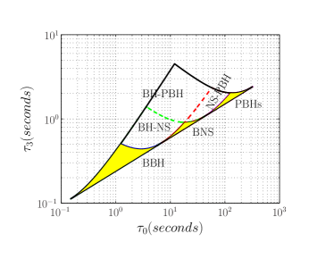
Figure 5: The parameter space of the search can be split into sub-spaces corresponding to astrophysically interesting binary sources. The left panel shows the parameter space of masses of the component stars for various astrophysically interesting systems while the right panel shows the same in the space of chirptimes. The properties of the compact object and the number of templates needed to cover these sub-spaces are quite different. The solid triangles on the left plot show sub-spaces where both the objects are of the same type and in the same mass range. The dashed squares show binary systems in which the two objects belong to different ranges of mass and are possibly of different type. While binary PBHs, BNS, BBH and BH-NS are all astrophysically possible, binaries where one of the components is a PBH and the other is a neutron star or a black hole probably don’t exist and need not be searched in the first instance. Note that in the space of chirptimes, where the area is proportional to the number of templates, these rather unrealistic systems occupy quite a large area and by excluding them in a search we can save significantly on the number of templates.

V.3.1 BNS case

First, we focus on the BNS case in which the mass range is set to 1-3 $M_{\odot}$. We plot bank efficiencies versus the total mass in Fig. 6. In these plots, we have combined the results of the 4 simulations involving GEO 600, LIGO-I, advanced LIGO and Virgo. In Fig. 7, we have separated the 4 results by plotting the cumulative histogram of the efficiencies. We can see that in all cases the safeness is above the minimal match: $\mathcal{S}_{10^{4}}=0.966,$ therefore the bank is efficient for the search of BNS. Furthermore, the cumulative histogram drops quickly while reaching the safeness. This is an indicator of the good behaviour of the bank. This also indicates that the bank is over-efficient and it is partly due to our choice of a rectangular, as opposed to a hexagonal, grid and partly due to the extra templates along the equal-mass curve.

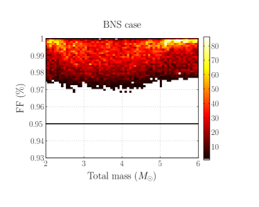
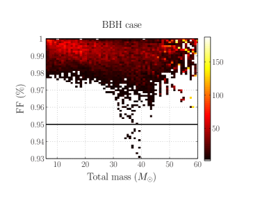
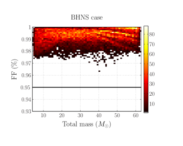
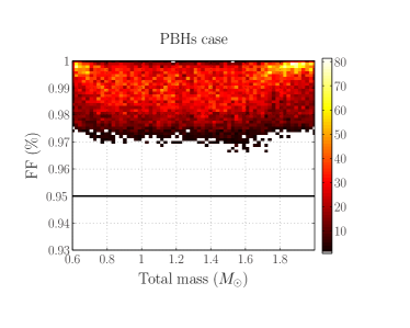
Figure 6: Distribution of the efficiency vectors versus total mass. The color bar on the right of each plot shows the number of recovered signals with given values of fitting factor and total mass.

V.3.2 Binary PBHs

The main difference compared to the BNS case is the number of templates. Indeed, we restrict the mass range to $[0.3-1]M_{\odot}$ and, therefore, the number of templates increases by a factor of 10. Results are summarised in Fig. 6 and Fig. 7. The conclusions are very similar to the BNS case. The safeness parameter is $\mathcal{S}_{10^{4}}=0.962$ and therefore the bank is efficient for the search of binary PBHs.

V.3.3 BBH case

The BBH search requires far fewer templates than in the case of binary PBHs or BNS. However, it is important to recall that the duration of the signal decreases as the chirp mass increases and there is a critical mass above which no signal enters the detector bandwidth. In the following simulations we restrict the upper mass to be 30 $M_{\odot}$.

By studying the results in Fig. 6 and 7 and Table 3, it is clear that the bank is efficient in the case of GEO 600, advanced LIGO and Virgo detectors, with the safeness equal to 0.973, 0.955 and 0.976, respectively, but in the LIGO-I case $\mathcal{S}<MM.$ From Fig. 6 we see that there are fewer than 1% of the injections that have a fitting factor below $MM.$ However, these few injections do have an overlap larger than 0.930. The injections that fail to achieve the required match are all concentrated in a specific region of the parameter space with their total mass between 30 and 40 $M_{\odot}$ as seen from Fig. 8. This is the region where the approximation that the signal manifold is flat breaks down and causes a “small hole” in template placement; but the effect is insignificant and does not deserve a fix. In any case, it is possible to use a larger $MM$ of the bank so as to capture these signals with the desired match. The increase in the number of templates is not a major issue since the number of templates in the BBH search is quite small compared to binary PBHs or BNS.

Table 3: Safeness parameter derived from the bank simulations.

Safeness $\mathcal{S}_{10^{4}}$ versus detector	GEO 600	LIGO-I	Advanced LIGO	VIRGO	all
BBH	0.973	0.931	0.955	0.976	0.931
BH-NS	0.977	0.964	0.972	0.970	0.964
BNS	0.970	0.972	0.968	0.966	0.966
Binary PBHs	0.968	0.968	0.969	0.962	0.962

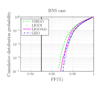
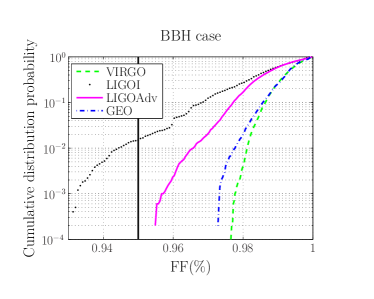
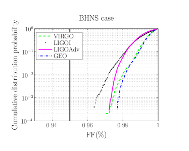
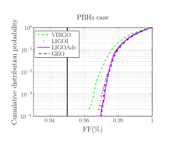
Figure 7: Panels from top-left to bottom-right summarize the cumulative distribution probability of the efficiency vector $\mathcal{E}$ for the different ranges of masses considered (namely, BNS, BBH, BH-NS and binary PBHs). Each panel has results from all the different detectors. While BNS, BH-NS and binary PBHs show a quadratic drop when FF drops closer to the minimal match, the BBH case shows a slower drop in the case of LIGO-I and advanced LIGO, with some values below the minimal match.

V.3.4 BH-NS case

Finally, we look at the BH-NS case. Here the component masses can take values in the range $[1-30]M_{\odot}$. There is an important issue here related to both the injections and ranges of masses in the template bank. First, since the BNS and BBH cases have already been studied independently, we do not need to look again at BBH or BNS systems. Therefore, we restrict $m_{1}\in[1-3]M_{\odot}$ and $m_{2}\in[3-60]M_{\odot}$. Second, the bank has to be extended up to 63 $M_{\odot},$ which is the sum of the maximum mass of the two objects. The safeness in this case is above the minimal match with a value $\mathcal{S}_{10^{4}}=0.964,$ which means that the proposed bank is efficient for the BH-NS search as well.

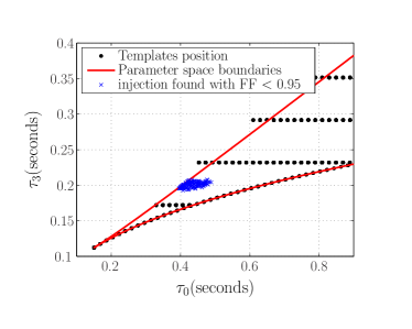
Figure 8: The bank designed for the LIGO-I design sensitivity curve covers the mass range [3-30] $M_{\odot},$ but there is a ‘hole’ in the parameter space corresponding to the total mass in the range $[30,\,40]M_{\odot}$. Black dots are where the templates are placed and crosses are the positions of the injected signals that have a fitting factor below the minimal match; majority of the injections are found with $FF>MM$ and are not plotted for the sake of clarity.

V.4 Taylor models

Finally, we perform two simulations, in the BBH and BNS case using only LIGO-I design sensitivity curve, in which both the templates and signals are based on the standard time-domain post-Newtonian model at 2PN order DIS2 . The parameters of the simulation are exactly the same as above. The results are shown in Fig. 9. As one can see, the recovered fitting factors are all above the $MM$ for both BNS and BBH, which means that the bank designed in this paper using the SPA models can be used for physical models based on Taylor approximants as well.

V.5 Computational cost

The algorithm presented in this paper is relatively fast. The computation time required to generate a template bank is of the order of a second to a few tens of seconds on any standard computer, depending on the parameters considered. Table 4 summarizes the computational cost needed to generate different template banks on a Linux Atlhon 1.6 GHz machine. The parameters used in these examples are similar to those in Ref. beauville , that is $F_{L}=30$ Hz, $f_{s}=4096$ Hz and $MM=0.95$ and a VIRGO PSD. The Table shows that a BBH template bank is created in a second while a template bank with $m_{\textrm{min}}=0.5M_{\odot}$ and $m_{\textrm{max}}=30M_{\odot}$ (more than 180,000 templates) required only 28 seconds. The number of templates quoted in Table 4 and in Ref. beauville are in very good agreement if we take into account a 30% effect coming from the fact that we used a square lattice instead of an hexagonal one.

Let us now consider our BBH template bank. The cost of matched filtering (to process 128 seconds of data through 2422 templates) is of the order of 50 minutes while the template bank generation costs 1 second. It is obvious that the template bank generation is a small fraction of the total cost.

Table 4: Computational cost for different template banks.

$m_{\textrm{min}}$	$m_{\textrm{max}}$	N	Time(s)
0.5	30	182137	28.0
1	3	10188	4.5
1	30	34905	6.0
3	30	2422	1.0

Since the placement uses a square lattice the number of templates is expected to be an extra 30% more in comparison to an hexagonal grid and the computational cost is larger by the same factor. Nowadays, analysing a month of gravitational wave data through $\approx 2000$ templates take a couple of days only depending on the number of computers used.

Decreasing the number of templates is, therefore, interesting especially in the BNS and PBH cases where the number of templates is large although this is not a major issue in the BBH case where it might even be safer to use a square lattice (see Sec. V.3.3). We provide an improvement of the algorithm presented in this paper by incorporating an hexagonal placement in a future work BCS2 .

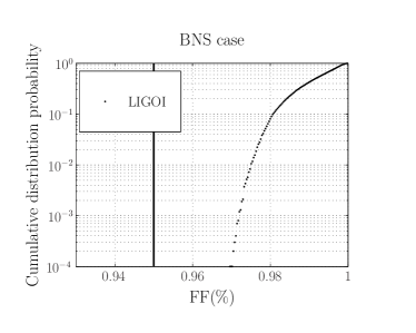
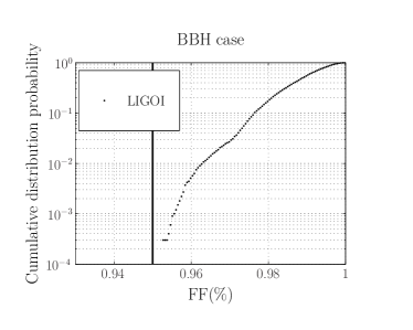
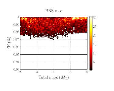
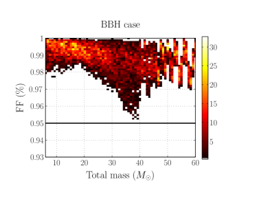
Figure 9: Cumulative distribution probability of the efficiency vectors $\mathcal{E}$ in the LIGO-I design sensitivity curve using a Taylor model instead of SPA both for templates and injected signals (top figures) and $\mathcal{E}$ distribution versus the total mass (bottom).

VI conclusion

In this paper we have used a geometrical method for constructing a template bank to search for gravitational waves from binary coalescences. The bank design is based on the Fourier-domain representation of the expected signal and the templates are placed on a square lattice. We have shown that the bank performs well with respect to its efficiency and safeness in the case of BNS, BH-NS and binary PBHs and for the 4 detectors considered and even over-efficient as expected since a square lattice has been used.

The proposed bank is also efficient in the case of BBH when the total mass is in the range [6-30] $M_{\odot}$. It remains efficient above 30 $M_{\odot}$ up to 60 in the case of VIRGO, advanced LIGO and GEO 600 detectors, the only problem being the case of LIGO-I in a specific total mass range of [30-40] $M_{\odot}$. This particular case has been investigated and correspond to the largest masses considered where the length of the signal is very short. Increasing the minimal match from 0.95 to 0.97 in the area which gives low match cures the problem. Therefore, we conclude that the square bank proposed is efficient for all the PSDs and searches we studied in this paper. We remind here that this bank has been used by the LIGO Scientific Collaboration to search for binary PBHs and BNS in four science runs LIGOS2bns ; LIGOS2bbh ; LIGOS2PBH .

Finally, it is important to emphasize that though we have been using signals and templates based on the SPA model, there is no restriction in using the same bank but for different models of signals and templates. Indeed, we have found that the current bank is efficient even when the signals and templates are both based on Taylor, Padé or EOB models (see Ref. DIS2 for model classification) as shown in a companion paper BCS2 ; in this paper we have also obtained a fast algorithm to construct a template bank on an hexagonal lattice with the number of templates reduced by $\approx 30\%$ (useful for the case of BNS and PBH searches where the number of templates could be very large).

Appendix A Placement algorithm

In this appendix we provide the algorithm used for the template placement described in Sec. IV. The algorithm is split into two distinct parts depending on the position in the parameter space.

In a nut-shell, the algorithm to lay templates along the equal-mass curve is as follows:

         Begin at $\tau_{0}=\tau_{0}^{\rm min}$
         do while $(\tau_{0}<\tau_{0}^{\rm max})$
         {
                 $\tau_{0}^{A}=\tau_{0}+\delta\tau_{0},\ \ \tau_{3}^{A}=4A_{3}\left({\tau_{0}^{A}}/{4A_{0}}\right)^{2/5}$
                 $\tau_{3}^{B}=\tau_{3}+\delta\tau_{3},\ \ \tau_{0}^{B}=4A_{0}\left({\tau_{3}^{B}}/{4A_{3}}\right)^{5/2}$
                 if ($(\tau_{0}^{A},\tau_{3}^{A})$ is closer to $(\tau_{0},\tau_{3})$ than $(\tau_{0}^{B},\tau_{3}^{B})$)
                 {
                          $\tau_{0}=\tau_{0}^{A},\tau_{3}=\tau_{3}^{A}$
                 }
                 else
                 {
                          $\tau_{0}=\tau_{0}^{B},\tau_{3}=\tau_{3}^{B}$
                 }
                 Add $(\tau_{0},\tau_{3})$ to InspiralTemplateList
                 numTemplates++
                 Compute metric at $(\tau_{0},\tau_{3})$
                 Compute distance between templates at new point:$(\delta\tau_{0},\delta\tau_{3})$
         }

The algorithm to lay templates in the rest of the parameter space is as follows:

         Begin at $\tau_{0}=\tau_{0}^{\rm min},\tau_{3}=\tau_{3}^{\rm min}$
         Compute metric at $(\tau_{0},\tau_{3})$
         Compute distance between templates at new point:$(\delta\tau_{0},\delta\tau_{3})$
         Add $(\tau_{0},\tau_{3})$ to InspiralTemplateList
         numTemplates++
         do while ($\tau_{3}<=\tau_{3}^{\rm max}$)
         {
                 Begin at $\tau_{0}=\tau_{0}^{\rm min}$
                 do while ($\tau_{0}<=\tau_{0}^{\rm max}$)
                 {
                          if ($(\tau_{0},\tau_{3})$ is inside the parameter space)
                          {
                                   Compute metric at ($\tau_{0},\tau_{3}$)
                                   Compute distance between templates at new point:($\delta\tau_{0},\delta\tau_{3}$)
                                   Add ($\tau_{0},\tau_{3}$) to InspiralTemplateList
                                   numTemplates++
                          }
                          Increment $\tau_{0}:$ $\tau_{0}=\tau_{0}+\delta\tau_{0}$
                 }
                 Increment $\tau_{3}:$ $\tau_{3}=\tau_{3}+\delta\tau_{3}$
                 Get next template along $\tau_{3}={\rm const.}$:$(\tau_{0},\tau_{3})$
         }

This algorithm is very simple to implement: except for the metric computation, the code is based on loops over simple calculations. It is a fast and robust algorithm amenable to easy implementation.

References

- (1) A. Abramovici et al., Science 256, 325 (1992); B. Abbott, et al., Nuclear Inst. and Methods in Physics Research, A 517/1-3 154 (2004).
- (2) H. Lück et al., Class. Quantum Grav. 14, 1471 (1997); ibid, 23, S71 (2006);
- (3) K. Tsubono, in First Edoardo Amaldi Conference on Gravitational Wave Experiments, (World Scientific, Singapore) p 112 (1995); K. Tsubono, et al., TAMA project, in The Ninth Marcel Grossman Meeting – Recent developments in theoretical and experimental general relativity, gravitation and relativistic field theories, (Eds. V.G. Gurzadyan, R.T. Jantzen and R. Ruffini) 145-154.
- (4) B. Caron et al., Class. Quantum Grav. 14, 1461 (1997); F. Acernese et al., The Virgo detector, Prepared for 17th Conference on High Energy Physics (IFAE 2005) (In Italian), Catania, Italy, 30 Mar-2 Apr 2005, AIP Conf. Proc. 794, 307-310 (2005).
- (5) L. Blanchet, T. Damour, B.R. Iyer, C.M. Will and A.G. Wiseman, Phys. Rev. Lett. 74, 3515 (1995).
- (6) L. Blanchet, T. Damour and B.R. Iyer, Phys. Rev. D 51, 5360 (1995).
- (7) L. Blanchet, G. Faye, B.R. Iyer, Jouguet, Phys. Rev. D 65, 061501(R) (2002).
- (8) L. Blanchet, B.R. Iyer, C.M. Will and A.G. Wiseman, Class. Quantum Grav. 13, 575, (1996).
- (9) L. Blanchet Living Rev. Rel. 5 (2003) gr-qc/0202016.
- (10) L. Blanchet, T. Damour, G. Esposito-Farese and B.R. Iyer Phys. Rev. Lett. 93 091101 (2004).
- (11) L.S. Finn, gr-qc/9609027; T. Nakamura, M. Sasaki, T. Tanaka, K.S. Thorne, Astrophys.J. 487, L139 (1997).
- (12) E. Poisson, Phys. Rev. D 52, 5719, (1995).
- (13) T. Damour, B. R. Iyer and B. S. Sathyaprakash Phys. Rev. D 57 885 (1998).
- (14) A. Buonanno and T. Damour Phys. Rev. D 59 084006 (1999).
- (15) A. Buonanno and T. Damour 62 064015 (2000).
- (16) T. Damour, P. Jaranowski and G. Schäfer Phys. Rev. D 62 084011 (2000).
- (17) T. Damour, B. R. Iyer and B. S. Sathyaprakash Phys. Rev. D 63 044023 (2001); Erratum-ibid, D 72 029902 (2005).
- (18) A. Buonanno, Y. Chen and M. Vallisneri, Phys. Rev. D 67 024016 (2003).
- (19) A. Buonanno, Y. Chen and M. Vallisneri, Phys. Rev. D 67 104025 (2003); Y. Pan, A. Buonanno, Y. Chen and M. Vallisneri, Phys. Rev. D 69 104017 (2004); A. Buonanno, Y. Chen, Y. Pan and M. Vallisneri, Phys. Rev. D 70 104003 (2004); A. Buonanno, Y. Chen, Y. Pan, H. Tagoshi and M. Vallisneri, Phys. Rev. D 72 084027 (2005);
- (20) P. Grandclement, V. Kalogera Phys. Rev. D 67 082002 (2003).
- (21) B. Allen, Phys. Rev. D 71 062001 (2005)
- (22) S. Babak, H. Grote, M. Hewitson, H. Lück, K.A. Strain, Phys. Rev. D72 022002 (2005)
- (23) B.S. Sathyaprakash and S.V. Dhurandhar, Phys. Rev. D 44, 3819 (1991).
- (24) S.V. Dhurandhar and B.S. Sathyaprakash, Phys. Rev. D 49, 1707 (1994).
- (25) R. Balasubramanian, B.S. Sathyaprakash, S.V. Dhurandhar Phys. Rev. D 53 3033 (1996); Erratum-ibid. D 54, 1860 (1996).
- (26) B. Owen, Phys. Rev. D53, 6749 (1996).
- (27) B. Owen, B. S. Sathyaprakash 1998 Phys. Rev. D 60 022002 (1998).
- (28) S. Babak, T. Cokelaer, B.S. Sathyaprakash, A. Sengupta, A template placement algorithm for the search of gravitational waves from inspiraling compact binaries II, in preparation.
- (29) B. Abbott et al., Phys. Rev. D72, 082001 (2005).
- (30) B. Abbott et al., Phys. Rev. D 73, 062001 (2006).
- (31) B. Abbott et al., Phys. Rev. D 72, 082002 (2005).
- (32) S.D. Mohanty, Phys. Rev. D 54, 7108 (1996).
- (33) C. Cutler and E.E. Flanagan, Phys. Rev. D 49, 2658 (1994).
- (34) D. Percival & A. Waldon Spectral analysis for physical applications, Cambridge University Press (1993).
- (35) E. Porter, Class. Quantum Grav. 19, 4343 (2002).
- (36) T.A. Apostalatos, Phys. Rev. D 52, 605 (1995).
- (37) B.F. Schutz, Data processing, analysis and storage for interferometric antennas, in The detection of gravitational waves edited by D.G. Blair, Cambridge University Press, 1991.
- (38) E. Poisson and C.M. Will, Phys. Rev. D 52, 848 (1995).
- (39) LSC Algorithm Library LAL , http://www.lsc-group.phys.uwm.edu/daswg/projects/lal.html
- (40) F. Beauville et al, Class. Quant. Grav. 22, 4285, (2005).
- (41) T. Tanaka and H. Tagoshi, Phys. Rev. D 62, 082001 (2000).
- (42) A. Lazzarini, S3 Best Strain Sensitivities, LIGO Document G040023-00-E.
- (43) B.J. Owen, private communication.
- (44) D. Brown, PhD Thesis, University of Wisconsin-Milwaukee (2004) (unpublished).