Cosmo-dynamics and dark energy with a quadratic EoS:
anisotropic models, large-scale perturbations and cosmological singularities

Abstract

In standard general-relativistic cosmology, for fluids with a linear equation of state (EoS) $P=w\rho$ or scalar fields, the high isotropy of the universe requires special initial conditions: singularities are velocity dominated and anisotropic in general. In brane world effective 4-dimensional cosmological models an effective term, quadratic in the energy density, appears in the evolution equations, which has been shown to be responsible for the suppression of anisotropy and inhomogeneities at the singularity under reasonable assumptions. Thus in the brane world isotropy is generically built in, and singularities are matter dominated. There is no reason why the effective EoS of matter should be linear at the highest energies, and an effective non-linear EoS may describe dark energy or unified dark matter (Paper I AB ). In view of this, here we investigate the effects of a quadratic EoS in homogenous and inhomogeneous anisotropic cosmological models in general relativity, in order to understand if in this standard context the quadratic EoS can isotropize the universe at early times. With respect to Paper I AB , here we use the simplified EoS $P=\alpha\rho+\rho^{2}/\rho_{c}$, which still allows for an effective cosmological constant and phantom behavior, and is general enough to analyze the dynamics at high energies. We first study homogenous and anisotropic Bianchi I and V models, focusing on singularities. Using dynamical systems methods, we find the fixed points of the system and study their stability. We find that models with standard non-phantom behavior are in general asymptotic in the past to an isotropic fixed point IS, i.e. in these models even an arbitrarily large anisotropy is suppressed in the past: the singularity is matter dominated. Using covariant and gauge invariant variables, we then study linear anisotropic and inhomogeneous perturbations about the homogenous and isotropic spatially flat models with a quadratic EoS. We find that, in the large scale limit, all perturbations decay asymptotically in the past, indicating that the isotropic fixed point IS is the general asymptotic past attractor for non phantom inhomogeneous models with a quadratic EoS.

I Introduction

Observations of large scale structure (LSS) LSS and cosmic microwave background radiation (CMBR) CMBR ; spergel ; WMAP3 indicate that the universe is highly homogenous and isotropic on large scales. Under standard assumptions on the matter content, in the standard general relativistic cosmological models isotropy is a special feature, requiring a high degree of fine tuning (a special set of initial conditions) in order to reproduce the observed universe. Specifically, in the set of spatially homogeneous cosmological models with a fluid which satisfy the energy conditions $\rho\geq|P|$ and $P\geq 0$, those which approach isotropy at late times is of measure zero CH . In these models the anisotropy dominates the dynamics in the neighborhood of the singularity, while the effect of matter is negligible: thus the singularity can be said to be velocity dominated ELS . In general anisotropic models do not isotropize sufficiently as they evolve into the future (models do not evolve towards a Friedmann-Robertson-Walker universe rapidly enough). This problem is known as the isotropy problem and can be solved by inflation. Many investigations on this issue show that a large class of models evolve towards a homogenous and isotropic model when under the influence of inflationary matter. This means that even models with initially high levels of anisotropy can evolve into the universe we observe today. A large body of work exists relating specifically to the study of spatially homogenous and anisotropic Bianchi cosmological models. In a classical paper, Wald showed that initially expanding Bianchi models with a cosmological constant asymptotically approach a de Sitter state (hence a spatially homogenous and isotropic model), except for the Bianchi type IX mixmaster models which may re-collapse RW . In the case of inhomogeneous models it is not so clear cut and in order for inflation to begin, sufficiently homogenous initial conditions are required (see e.g. KT ; BMP ). As far as singularities in general relativity are concerned, it is widely accepted Garfinkle that the Belinskii, Khalatnikov and Lifshitz (BKL) BKL ; LL picture is correct: for fluids with linear EoS $P=w\rho$ ($w<1$) or scalar fields, when the singularity of generic inhomogeneous anisotropic cosmological models is approached, the dynamics is asymptotically that of the mixmaster model, the singularity is thus velocity dominated and the effect of matter is negligible Ashtekar .

More recently various theories of gravity that go beyond general relativity have been considered. For instance, high energy modifications of gravity could come from extra dimensions (as required in string theory). In the brane world SMS ; BMW ; DL ; RM scenario the extra dimensions produce a term quadratic in the energy density in the 4-dimensional effective energy-momentum tensor, i.e. this quadratic term appears in the 4-d evolution and constraint equations on the brane. Under the reasonable assumption of neglecting 5-d Weyl tensor contributions in these equations, this quadratic term has the very interesting effect of suppressing anisotropy at early enough times, as the singularity is approached. In the case of a Bianchi I brane-world cosmology containing a scalar field with a large kinetic term the initial expansion is quasi-isotropic MSS . In this scenario, the initial anisotropy provides increased damping in the scalar field equation of motion, thus resulting in an extended period of inflation. The rapid decay of the anisotropy results in the class of initial conditions allowed by observations to be greatly increased. Under the same assumptions, Bianchi I and Bianchi V brane-world cosmological models containing standard cosmological fluids with linear equation of state (EoS) ($P/\rho=w>0$) also behave in a similar manner CS . The same is also true for more general homogeneous models coley1 ; coley2 and even some inhomogeneous exact solutions coley3 . Finally, within the limitations of a perturbative treatment, the quadratic-term-dominated isotropic brane-world models have been shown to be local past attractors in the larger state space of inhomogeneous and anisotropic models DGBC ; GDCB . More precisely, again assuming that the 5-d Weyl tensor contribution to the brane can be neglected, large-scale perturbations of the isotropic models vanish in the past, approaching the singularity. Large scale perturbations $\lambda\gg H^{-1}$ are the only type relevant to this kind of analysis for non-inflationary matter, because for any given $\lambda$ there is always an early enough time such that $\lambda\gg H^{-1}$ is satisfied. Thus in the brane scenario the observed high isotropy of the universe is built in, i.e. the natural outcome of generic initial conditions, unlike in general relativity where general cosmological models with a linear EoS are highly anisotropic in the past, approaching the singularity a-la BKL, i.e. with mixmaster dynamics BKL ; LL ; Ashtekar .

It would therefore be interesting to see if the behavior of the anisotropy at the singularity found in the brane scenario is recreated in the general relativistic context if we consider a quadratic term in the EoS. That is, do we have a scenario where, in general relativity, the generic asymptotic attractor in the past is an isotropic model, thanks to a non-linear EoS. This is the question we aim to investigate, for the specific case of the EoS $P=\alpha\rho+\rho^{2}/\rho_{c}$. This is a simplified version of that used in Paper I AB , where the focus was on using a quadratic EoS to represent a dark energy component or unified dark matter. It is general enough to analyze the high energy dynamics we are interested here, while still allowing for an effective cosmological constant and phantom behavior.

The paper is organized as follows. In section II we outline the setup of the models under investigation, defining three classes, one of which represents a fluid with phantom behavior. Using dynamical system methods WE ; AP , in section III we consider the anisotropic Bianchi I and V class of homogenous models containing a perfect fluid with quadratic EoS, showing how models with standard non-phantom matter are asymptotic in the past to an isotropic fixed point IS. Using covariant and gauge invariant variables EB ; BDE ; VEE , in section IV we give the linearized evolution and constraint equations for generic inhomogeneous and anisotropic perturbations about a flat Friedmann model with a quadratic EoS. We solve the equations in the large scale limit $\lambda\gg H^{-1}$ and show that the perturbations vanish as the singularity is approached, indicating that the isotropic model IS is the generic past attractor. We then finish with some concluding remarks and discussion in section V.

II The model

We begin with a summary of the most relevant points that can be derived mostly from an analysis of energy conservation alone. More details can be found in Section II in Paper I AB .

The energy conservation equation for a cosmological model containing a perfect fluid is:

$$\dot{\rho}=-3H(\rho+P),$$ (1)

where $\rho$ is the energy density, $P$ the isotropic pressure and $H$ is the Hubble expansion scalar. An average scale factor $a$ is defined, at least locally, by $\dot{a}/{a}\equiv H$. Through this relation solutions of Eq. (1) can be found in terms of $a$, but first an EoS must be specified. Usually this is taken to be a linear function of the energy density of the form $P=w\rho$, with $w=constant$. In this case Eq. (1) gives:

$$\rho = \rho_{o}\left(\frac{a}{a_{o}}\right)^{-3(w+1)}.$$ (2)

In the case of the homogenous and anisotropic Bianchi I cosmological models, the amplitude of the shear scales as:

$$\sigma^{2} = \sigma_{o}^{2}\left(\frac{a}{a_{o}}\right)^{-6}.$$ (3)

This example shows how the shear can decay rapidly in an expanding model, growing larger for smaller $a$. If the dynamics of the model is such that $a\rightarrow 0$, both $\rho$ and $\sigma$ blow up, and the model has a physical singularity. In the case $w<-1$, the so called “phantom” fluid Caldwell , the energy density counter intuitively decays (grows) in the past (future) and therefore any shear component always comes to dominate at the initial “Big Bang” singularity. In the case when $-1\leq{\it w}<1$ the energy density decays during expansion, but at a slower rate than the shear, so that once again the shear component dominates at the singularity. In approaching these singularities matter with linear EoS $w<1$ is un-influential, therefore these singularities may be termed velocity dominated ELS . It is only in the case when $w>1$ (“super-stiff” fluid) that the energy density is dominant in the past and therefore the initial singularity is isotropic. This indicates that as the initial singularity is approached in the standard homogenous model with $w<1$, any residual anisotropy will generally come to dominate near the singularity. The anisotropy is a generic feature of these models and the initial singularity is in general anisotropic and velocity dominated.

As discussed earlier, motivated by the results in the brane-world models, we aim to investigate the effects of introducing a non-linear EoS on the behavior of anisotropic models. The EoS we propose is quadratic in the energy density (we neglect the constant pressure term introduced in Paper I AB as in general this only modifies late time behavior):

$$P=\alpha\rho+\frac{\epsilon\rho^{2}}{\rho_{c}}.$$ (4)

The discrete parameter $\epsilon$ denotes the sign of the quadratic term, $\epsilon\in\{-1,1\}$, and $\rho_{c}>0$ sets the energy scale above which this term becomes relevant. The energy conservation equation (1) can now be integrated to give the scaling of the energy density as a function of the scale factor (except for $\alpha=-1$).

$$\rho = \frac{A(\alpha+1)\rho_{c}}{a^{3(\alpha+1)}-\epsilon A},$$ (5)

$$A = \frac{\rho_{o}a_{o}^{3(\alpha+1)}}{(\alpha+1)\rho_{c}+\epsilon\rho_{o}}.$$ (6)

where $\rho_{o}$, $a_{o}$ represent the energy density and scale factor at an arbitrary time $t_{o}$. This is valid for all values of $\epsilon$, $\rho_{c}$ and $\alpha$ ($\alpha\neq-1$). Defining

$$\rho_{\Lambda}\equiv-\epsilon(1+\alpha)\rho_{c}$$ (7)

the fluid admits an effective positive cosmological constant point, $\rho_{\Lambda}>0$, only if $\epsilon(1+\alpha)<0$. As shown in Paper I AB , in the case of $\epsilon=-1$ the fluid generally behaves either in a phantom manner or is asymptotic to a finite energy density in the past, the effective cosmological constant $\rho_{\Lambda}$, for all open and flat models. In this scenario, the initial singularity is going to be dominated by anisotropic expansion as seen in the standard linear EoS case, due to the sub-dominance of the energy density at early times; therefore we do not consider the $\epsilon=-1$ case further.

In the case of $\epsilon=+1$, the expression (5) for the energy density $\rho(a)$ is conveniently rewritten in three different ways, defining $a_{\star}=|A|^{1/3(\alpha+1)}$ and assuming $\rho>0$.

A: $(1+\alpha)>0$, $\rho_{\Lambda}<0$,

$$\rho=\frac{(1+\alpha)\rho_{c}}{\left(\frac{a}{a_{\star}}\right)^{3(1+\alpha)}-1}.$$ (8)

In this case $a_{\star}<a<\infty$, with $\infty>\rho>0$. The past singularity is similar to certain future singularities found in dark energy models NOT ; barrow and is referred to as Type III singularities:

• For $t\to t_{\star}$, $a\to a_{\star}$, $\rho\to\infty$ and $|P|\to\infty$

Where $t_{\star}$ and $a_{\star}$ are constants with $a_{\star}\neq 0$ (we reach $a_{*}$ at a finite $t_{*}$). The main difference is that in our case the singularity occurs in the past. At late times the fluid behaves in a similar manner to a fluid with a linear EoS and $w=\alpha$.

B: $(1+\alpha)<0$, $0<\rho_{\Lambda}<\rho$,

$$\rho=\frac{\rho_{\Lambda}}{1-\left(\frac{a}{a_{\star}}\right)^{3(1+\alpha)}}.$$ (9)

In this case $a_{\star}<a<\infty$, with $\infty>\rho>\rho_{\Lambda}$. As in case A, the fluid approaches a Type III singularity in the past, but now approaches an effective cosmological constant at late times.

C: $(1+\alpha)<0$, $0<\rho<\rho_{\Lambda}$,

$$\rho=\frac{\rho_{\Lambda}}{1+\left(\frac{a}{a_{\star}}\right)^{3(1+\alpha)}}.$$ (10)

In this case $0<a<\infty$, with $0<\rho<\rho_{\Lambda}$. The fluid behaves in a phantom manner but tends to an effective cosmological constant at late times.

In the cases A and B, as we approach the past singularity the energy density approaches infinity, in fact the singularity occurs at a finite scale factor, that is for the energy density one has $\rho\to\infty$ as $a\to a_{\star}$. The cosmological model emerges at a finite scale factor $a_{\star}$, with infinite energy density and infinite isotropic pressure $P$. The model emerges from a curvature singularity, infinitely decelerates and asymptotically approaches a standard flat Friedmann model with a linear EoS (case A) or a de Sitter model (case B). In the case C, the fluid behaves in a phantom manner and approaches $\rho_{\Lambda}$ at late times. In this case the energy density is sub-dominant at early times and the anisotropy will dominate as we will show in the proceeding sections. In cases A and B, we have the possibility that the energy density could be the dominant component in the past, forcing the singularity to be isotropic. This would result in isotropic expansion at early times as seen in the brane-world model, with the fluid also approaching a non super-stiff EoS at late times. We will now proceed with the analysis of anisotropic cosmological models containing a fluid with a quadratic EoS.

III Dynamics of Bianchi models

We now study the dynamics of homogeneous and anisotropic Bianchi cosmological models. In particular we investigate the Bianchi I and V classes of models that contain the flat and open Friedmann models. The matter content will be modeled by a non-tilted (that is the fluid flow remains orthogonal to the group orbits) perfect fluid with a quadratic EoS.

We make use of the orthonormal frame formalism which results in a system of first-order evolution equations. We have adopted a notation consistent with that used in WE (Greek indices run from $\alpha=1,\ldots,3$ and Latin indices run from $i=0,\ldots,3$). The orthonormal frame formalism is a 1+3 decomposition of the Einstein field equations into evolution and constraint equations. The decomposition is carried out relative to the time-like vector field ${\bf{e}}_{0}$ of a given orthonormal frame $\{{\textbf{e}}_{i}\}$. In the case of models which admit an isometry group, ${\bf{e}}_{0}$ is chosen to be the normal (${\bf u}$) to the space-like group orbits. The Bianchi models are such cosmological models, they admit a three dimensional group of isometries which act simply and transitively on the space-like hyper-surfaces (surfaces of homogeneity). The orthonormal frame $\{{\bf u},{\bf e}_{\alpha}\}$, is such that:

$$\textbf{u}\cdot\textbf{u}=-1,\qquad\textbf{u}\cdot{\textbf{e}}_{\alpha}=0,\qquad{\textbf{e}}_{\alpha}\cdot{\textbf{e}}_{\beta}=\delta_{\alpha\beta}.$$ (11)

The dynamics can then be described in terms of the spatial commutation functions, the kinematical quantities and the matter variables. The spatial commutation functions, $\gamma^{\alpha}{}_{{\beta}{\mu}}$, are defined by the commutation relations between the spatial basis vectors such that:

$$[{\textbf{e}}_{\alpha},{\textbf{e}}_{\beta}]=\gamma^{\mu}{}_{{\alpha}{\beta}}{\textbf{e}}_{\mu}.$$ (12)

The spatial commutation functions can be decomposed into a $2$-index symmetric object and a $1$-index object which determine the connections on the space-like 3-surfaces.

$$\gamma^{\alpha}{}_{{\beta}{\mu}}=\varepsilon_{{\beta}{\mu}{\nu}}n^{{\alpha}{\nu}}+a_{\beta}\delta_{\mu}{}^{\alpha}-a_{\mu}\delta_{\beta}{}^{\alpha}.$$ (13)

The kinematical quantities include the Hubble scalar $H$, the shear tensor $\sigma_{{\alpha}{\beta}}$ and the angular velocity $\Omega_{\alpha}$, relative to a Fermi-propagated spatial frame, of the spatial frame $\{{\textbf{e}}_{\alpha}\}$ along the time-like vector ${\bf u}$. The relevant matter variables are the energy density $\rho$ and the isotropic pressure $P$, while the energy flux and the anisotropic pressure are set to zero as we are considering a perfect fluid. The decomposed Einstein field equations for a general Bianchi model containing a perfect fluid then take the form:

$$\dot{H} = -H^{2}-\frac{2}{3}\sigma^{2}-\frac{1}{6}(\rho+3P),$$ (14)

$${\dot{\sigma}}_{{\alpha}{\beta}} = -3H{\sigma}_{{\alpha}{\beta}}-^{(3)}{S_{{\alpha}{\beta}}}$$ (15)

$$+2\Omega_{\nu}(\varepsilon^{{\mu}{\nu}}{}_{{\alpha}}\sigma_{{\beta}{\mu}}+\varepsilon^{{\mu}{\nu}}{}_{{\beta}}\sigma_{{\alpha}{\mu}}),$$

$$\rho = 3H^{2}-{\sigma}^{2}+\frac{1}{2}{{}^{(3)}{R}},$$ (16)

$$0 = 3{\sigma}_{\alpha}{}^{\beta}a_{\beta}-\varepsilon_{\alpha}{}^{{\beta}{\mu}}{\sigma}_{\beta}{}^{\nu}n_{{\nu}{\mu}}.$$ (17)

The trace-free spatial Ricci tensor (${}^{3}{S_{{\alpha}{\beta}}}={}^{3}{R_{{\alpha}{\beta}}}-\frac{1}{3}~{}{}^{3}{R}\delta_{\alpha\beta}$) and the spatial curvature scalar (${}^{3}{R}={}^{3}{R_{\alpha}^{\alpha}}$) can be given in terms of the spatial commutation functions:

$${}^{3}{S_{{\alpha}{\beta}}} = b_{{\alpha}{\beta}}-\frac{1}{3}(b_{\mu}{}^{\mu})\delta_{{\alpha}{\beta}}$$ (18)

$$-2a_{\nu}(\varepsilon^{{\nu}{\mu}}{}_{{\alpha}}n_{{\beta}{\mu}}+\varepsilon^{{\nu}{\mu}}{}_{{\beta}}n_{{\alpha}{\mu}}),$$

$${}^{3}{R} = -\frac{1}{2}b_{\mu}{}^{\mu}-6a_{\mu}a^{\mu}.$$ (19)

The quantity $b_{{\alpha}{\beta}}$, can be expressed in terms of the spatial commutation functions and has the form:

$$b_{{\alpha}{\beta}}=2n_{\alpha}{}^{\mu}n_{{\mu}{\beta}}-n_{\mu}{}^{\mu}n_{{\alpha}{\beta}}.$$ (20)

The Jacobi identity for vector fields when applied to the spatial frame vectors ${\textbf{e}}_{\alpha}$, in conjunction with the Einstein field equations give a set of evolution and constraints equations:

$${\dot{n}}_{{\alpha}{\beta}} = -H{n}_{{\alpha}{\beta}}+2(\sigma_{\alpha}{}^{\mu}n_{{\beta}{\mu}}+\sigma_{\beta}{}^{\mu}n_{{\alpha}{\mu}})$$ (21)

$$+2\Omega_{\nu}(\varepsilon^{{\mu}{\nu}}{}_{{\alpha}}\sigma_{{\beta}{\mu}}+\varepsilon^{{\mu}{\nu}}{}_{{\beta}}\sigma_{{\alpha}{\mu}}),$$

$${\dot{a}}_{\alpha} = -Ha_{\alpha}-{\sigma}_{\alpha}{}^{\beta}a_{\beta}+\varepsilon_{\alpha}{}^{{\mu}{\nu}}a_{\mu}\Omega_{\nu},$$ (22)

$$0 = n_{\alpha}{}^{\beta}a_{\beta}.$$ (23)

The evolution equation for the energy density results from the contracted Bianchi identities, or more directly from the conservation equations, and has the form (1). The latter with the above system of equations reduce to the evolution and constraint equations for given non-tilted perfect fluid Bianchi model by making further restrictions on the spatial commutation functions ($n_{\alpha\beta}$,$a_{\alpha}$) and kinematical quantities ($\sigma_{\alpha\beta}$,$\Omega_{\alpha}$). The Bianchi I and V models are considered separately in the following sub-sections.

III.1 Bianchi I cosmologies

The Bianchi I models are a subclass of the Bianchi Class A models ($a_{\alpha}=0$). These models are homogeneous and anisotropic cosmological models containing the flat Friedmann (F) model. In the case of Bianchi I, the group invariant orthonormal frame $\{{\bf u},{\bf e}_{\alpha}\}$ can be further specialized such that:

$$a_{\alpha}=n_{\alpha\beta} = 0,$$ (24)

$$\gamma^{\mu}{}_{\alpha\beta} = 0.$$ (25)

This in turn means that the three curvature of the spatial hyper-surfaces (18, 19) is zero:

$${}^{(3)}{R}_{\alpha\beta} = 0.$$ (26)

The Einstein field equations (15, 17) and the Jacobi identity (21) imply:

$$\sigma_{{\alpha}{\beta}}=diag(\sigma_{11},\sigma_{22},\sigma_{33}),\qquad\Omega_{\alpha}=0.$$ (27)

The analysis of the system of equations can be simplified by introducing the following set of normalized dimensionless variables:

$$x=\frac{\rho}{\rho_{c}}~{},\qquad y=\frac{H}{\sqrt{\rho_{c}}}~{},$$

$$z=\frac{\sigma}{\sqrt{\rho_{c}}}~{},\qquad\eta=\sqrt{\rho_{c}}t~{},$$ (28)

where $\sigma\equiv\sqrt{\sigma_{\alpha\beta}\sigma^{\alpha\beta}/2}$. In addition, it is customary to introduce

$$\Sigma=\frac{\sigma}{H}=\frac{z}{y}$$ (29)

as a dynamically dimensionless measure of anisotropy: we can refer to a cosmological model as isotropic in some limit if, in that limit, $\Sigma\rightarrow 0$. In particular, if there is a singularity for some $a_{s}$ (possibly zero), we refer to the singularity as isotropic if $\Sigma\rightarrow 0$ in the limit $a\rightarrow a_{s}$.

The above normalization to $\rho_{c}$ is useful because the energy scale $\rho_{c}$ itself disappears from the dynamical system: in terms of the dimensionless variables above, the complete system of equations for Bianchi I models is explicitly made scale invariant, and is:

$$y^{2} = \frac{x}{3}+\frac{z^{2}}{3},$$ (30)

$$x^{\prime} = -3y\left((\alpha+1)x+x^{2}\right),$$ (31)

$$y^{\prime} = -y^{2}-\frac{1}{6}\left((3\alpha+1)x+3x^{2}\right),$$ (32)

$$z^{\prime} = -3yz.$$ (33)

The primes denote differentiation with respect to $\eta$, the normalized time variable. The variable $x$ is the normalized energy density, $y$ is the normalized Hubble scalar and $z$ is the normalized shear. The effective cosmological constant point is now given by $x_{\Lambda}=-(1+\alpha)$. We only consider the region of the state space for which the energy density remains positive ($x\geq 0$) and models which are expanding ($y\geq 0$). The evolution equation for the shear can be integrated to give:

$$z=z_{o}\left(\frac{a}{a_{o}}\right)^{-3}~{}.$$ (34)

The shear tends to grow in the past and rapidly decays at late times. Using Eqs. (8), (9), (10) and (34) we can see how the shear scales with respect to the energy density (by substituting for the scale factor in each case) for each of the three sub-cases of the fluid.

Case A: $(1+\alpha)>0$, $\rho_{\Lambda}<0$,

$$z=z_{o}\left(\frac{x}{|\alpha+1|+x}\right)^{\frac{1}{|\alpha+1|}}.$$ (35)

In this case, at early times the energy density diverges, $x\to\infty$ and the shear goes to a constant value, $z\to z_{o}$. The initial singularity is dominated by the energy density and is forced to be isotropic, as $\Sigma\to 0$. At late times, $x\to 0$ and $z\to 0$.

Case B: $(1+\alpha)<0$, $0<\rho_{\Lambda}<\rho$,

$$z=z_{o}\left(\frac{x-x_{\Lambda}}{x}\right)^{\frac{1}{|\alpha+1|}}.$$ (36)

In this case, at early times the energy density diverges, $x\to\infty$; the shear goes to a constant, $z\to z_{o}$. The initial singularity is again dominated by the energy density and is forced to be isotropic, with $\Sigma\rightarrow 0$. At late times the energy density approaches a constant value, $x\to x_{\Lambda}$ and $z\to 0$.

Case C: $(1+\alpha)<0$, $0<\rho<\rho_{\Lambda}$,

$$z=z_{o}\left(\frac{x_{\Lambda}-x}{x}\right)^{\frac{1}{|\alpha+1|}}.$$ (37)

In the final case, the fluid behaves in a phantom manner. At early times $x\to 0$ and $z\to\infty$. The initial singularity is now dominated by the shear and is anisotropic. At late times the energy density approaches a constant value, $x\to x_{\Lambda}$ and $z\to 0$.

In cases A and B we expect the generic past attractor to be an isotropic singularity, while at late times we expect either a Minkowski or de Sitter model to be the attractor. In case C, the fluid behaves in a phantom manner and we expect models to be asymptotic to a anisotropic singularity in the past and a de Sitter model in the future. We now carry out a dynamical systems analysis of the above system. The system can be reduced from a 3D system to a 2D system by substituting for a variable using the generalized Friedmann equation (30). We choose to remove the normalized Hubble scalar $y$, assuming expansion, $y>0$. The resulting reduced planar dynamical system is then:

$$x^{\prime} = -\sqrt{3(x+z^{2})}\left((\alpha+1)x+x^{2}\right),$$ (38)

$$z^{\prime} = -\sqrt{3(x+z^{2})}z.$$ (39)

The above system of equations is of the form $u^{\prime}_{i}=f_{i}(u_{j})$. Since this system is autonomous, trajectories in state space connect the fixed/equilibrium points of the system ($u_{j,o}$), which satisfy the system of equations $f_{i}(u_{j,0})=0$. The stability nature of the fixed points can be found by carrying out a linear stability analysis, see Section II.B in Paper I AB for a summary, and e.g. WE ; AP for more details. The fixed points of the reduced planar system (38)-(39), the corresponding eigenvalues and there existence conditions (the energy density remains positive ($x\geq 0$) and all three variables are real ($x,~{}y,~{}z\in\mathbb{R}$)) are given in Table 1.

Table 1: Location, eigenvalues and existence conditions ($x\geq 0$ and $x,~{}y,~{}z\in\mathbb{R}$) for the fixed points of the reduced Bianchi I planar system (38)-(39). To simplify we use $\tau=-(\alpha+1)$.

Name	$x$, $z$	Eigenvalues	Existence
M	($0$, $0$)	$0$, $0$	$\alpha\in\mathbb{R}$
dS	($\tau$, $0$)	$-\tau\sqrt{3\tau}$, $-\sqrt{3\tau}$	$\alpha<-1$

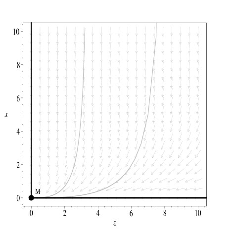
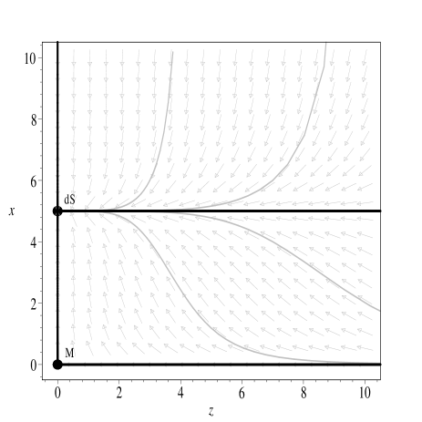
Figure 1: The state space for the Bianchi I reduced planar system (38)-(39), showing fixed points at finite values of the energy density and shear. (a) Left panel: the state space for $\alpha>-1$; the only fixed point present represents a Minkowski model. (b) Right panel: the state space for $\alpha<-1$; in this case there is a new fixed point dS which represents a flat expanding de Sitter model with $\rho_{\Lambda}=-(1+\alpha)\rho_{c}$. The separatrix represents models with $\rho=\rho_{\Lambda}$. Models below this line have phantom behavior.

The first point represents the vacuum static Minkowski model. Eigenvalues of the linearized system are zero, hence the linearization theorem AP doesn’t apply at this point and we resort to numerical analysis to determine the stability character. In the case $\alpha>-1$, this is the only finite valued fixed point present. This is clearly seen in Fig. 1(a), corresponding to case A, where the black lines represent separatrices, the dots represent fixed points and the thin grey lines are example trajectories. The Minkowski point M is clearly the future attractor for all trajectories in the region. The behavior in the past is not clear from this diagram (but trajectories do appear to evolve to a constant $z$). The horizontal black line represents the Bianchi I Kasner vacuum models, with line element:

$$ds^{2}=-dt^{2}+t^{2p_{1}}dx_{1}^{2}+t^{2p_{2}}dx_{2}^{2}+t^{2p_{3}}dx_{3}^{2}.$$ (40)

The parameters $p_{\alpha}$ satisfy the following constraints:

$$\sum_{n=1}^{3}p_{n}=1,\qquad\sum_{n=1}^{3}p_{n}^{2}=1,$$ (41)

and the average scale factor for expanding models of this type is given by:

$$a=a_{o}(\eta-\eta_{o})^{1/3}.$$ (42)

Although these models are asymptotic to Minkowski at late times, as seen in Fig.  1(a), they are always anisotropic, in the sense that $\Sigma=\sqrt{3}$ at all times. The Kasner singularity is a paradigmatic, characteristic of many models; the more general Bianchi IX singularity is approximated by a series of jumps from a Kasner phase to another, see e.g. LL ; WE . The vertical black line represents the expanding flat Friedmann model with a quadratic EoS. In the case of a spatially flat model as in this case, the Friedmann equation can be integrated to give the dependence of the scale factor on time:

$$\eta = \frac{6}{[3(\alpha+1)]^{3/2}}\times\left\{\sqrt{(a/a_{\star})^{3(\alpha+1)}-1}\right.$$ (43)

$$\left.-\arctan\left(\sqrt{{(a/a_{\star})^{3(\alpha+1)}-1}}\right)\right\}$$

The scale factor starts at finite size $a_{\star}$ (we have fixed constants so that this corresponds to $\eta_{\star}=0$), expands and asymptotically approaches the behavior of a model with the standard linear EoS,

$$a\approx a_{\star}(\eta-\eta_{o})^{2/3(\alpha+1)}.$$ (44)

For $\alpha<-1$, Fig. 1(b), there is a second fixed point dS representing the generalized flat expanding de Sitter model. This point has attractor stability character, i.e. in this case the generalized de Sitter model is the generic future attractor. The new horizontal black line in Fig. 1(b) is a separatrix representing models with $x_{\Lambda}=-(\alpha+1)$; it is the dividing line between the phantom ($x<x_{\Lambda}$) and standard behavior ($x>x_{\Lambda}$). The trajectories below this line represent phantom models (corresponding to case C), that is the energy density increases as the model expands. The models in this region appear to be dominated by shear in the past ($x\to 0$, $z\to\infty$ as $\eta\to-\infty$) and asymptotically approach a de Sitter model in the future ($x\to x_{\Lambda})$, $z\to 0$ as $\eta\to\infty$). The scale factor for an expanding flat de Sitter model has the form:

$$a=a_{o}e^{(\eta-\eta_{o})}.$$ (45)

The trajectories above the separatrix (corresponding to case B) also asymptotically approach the generalized de Sitter model in the future.

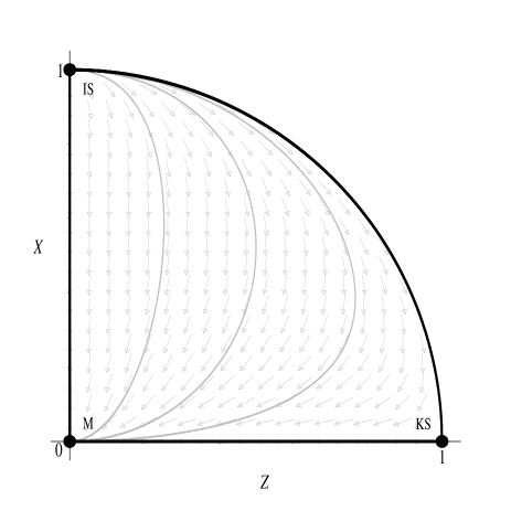
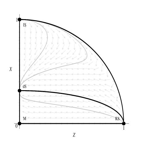
Figure 2: The compactified state space ($X$, $Z$) for the Bianchi I reduced system, including fixed points at infinity. These represent the isotropic singularity (IS) and the Kasner anisotropic singularity (KS). (a) Left panel: the state space for $\alpha>-1$, corresponding to case A, Fig. 1(a). (b) Right panel: the state space for $\alpha<-1$. The separatrix corresponds to that of Fig. 1(b), with $\rho=\rho_{\Lambda}$. Above this line we have models of type B. Models below this line are phantom, of type C, and Kasner-like at the singularity KS. Clearly the non-phantom models of type A and B are asymptotic to the IS fixed point in the past.

The behavior in the past is not clear from the state space in Fig. 1. In order to analyze the dynamics at infinity, we introduce compactified Poincaré variables ${X}_{i}$; these can be expressed in terms of the standard variables $x_{i}$ as:

$${X}_{i} = \frac{x_{i}}{\sqrt{1+{\sum_{i=1}^{n}x_{i}^{2}}}}.$$ (46)

The relationship can be inverted to give:

$$x_{i} = \frac{{X}_{i}}{\sqrt{1-{\sum_{i=1}^{n}{X}_{i}^{2}}}}.$$ (47)

The new variables allow one to analyze the dynamics at infinity more easily, as $x_{i}\to\infty\Rightarrow{X}_{i}\to 1$. The evolution equations for the new variables are then given by:

$${X}_{i}^{\prime} = \sqrt{1-{\sum_{j=1}^{n}{X}_{j}^{2}}}\left(x_{i}^{\prime}-{X}_{i}{\sum_{k=1}^{n}~{}{X}_{k}~{}x_{k}^{\prime}}\right),$$ (48)

where the $x_{i}^{\prime}$ represent the evolution equations for the original variables. We now study the compactified and reduced system ($X$, $Z$); the fixed points of the system are given in Table 2.

The first two fixed points (M and dS) represent the Minkowski and generalized de Sitter points as in the non-compactified case and retain the same stability character. The third point (IS) represents the isotropic singularity, which is matter dominated ($X\to 1$, or $x\to\infty$). This fixed point always has repeller stability and is the generic past attractor. The final fixed point (KS) represents the anisotropic Kasner singularity ($Z\to 1$, or $z\to\infty$). This fixed point has saddle stability. The full state space for the system can now be reconstructed, and is depicted in Fig. 2, where as before the black lines represent separatrices, the dots represent fixed points and the thin grey lines are example trajectories.

Table 2: Location and existence conditions ($X\geq 0$ and $X,~{}Z\in\mathbb{R}$) for the compactified planar Bianchi I system. To simplify we use $\tau=-(\alpha+1)$. The * is shown when the point does not exist.

Name	$X$, $Z$	Existence	Stability ($\alpha<-1,~{}\alpha>-1$)
M	($0$, $0$)	$\alpha\in\mathbb{R}$	Saddle, Attractor
dS	$\left(\frac{\tau}{\sqrt{1+\tau^{2}}},~{}0\right)$	$\alpha<-1$	Attractor, *
IS	($1$, $0$)	$\alpha\in\mathbb{R}$	Repeller, Repeller
KS	($0$, $1$)	$\alpha\in\mathbb{R}$	Saddle, Saddle

In the case $\alpha>-1$, Fig. 2(a) (this corresponds to case A, i.e. this is the compactified version of Fig. 1(a)), there are three fixed points, M, IS and KS. The horizontal black line $X=0$ represents the anisotropic Kasner model. The vertical black line $Z=0$ represents the flat Friedmann model containing a fluid with a quadratic EoS. The Minkowski point M is the future attractor for all trajectories in the region. The isotropic singularity IS is the generic past attractor and the anisotropic Kasner singularity KS has saddle stability character. The set of initial conditions for which anisotropy dominates in the past are special, corresponding to vacuum models $X=0$, as opposed to being generic as in the case of the linear EoS.

In the case $\alpha<-1$, Fig. 2(b), there are four fixed points, M, dS, IS and KS. The state space is split into two regions by the separatrix joining the points dS and KS and given by $X=X_{\Lambda}$, where:

$$X_{\Lambda} = \tau\sqrt{\frac{1-Z^{2}}{1+\tau^{2}}}.$$ (49)

and $\tau=-(\alpha+1)$. In the region above the separatrix ($X>X_{\Lambda}$, corresponding to case B) the fluid behaves in a standard manner. The IS fixed point has repeller stability character and all trajectories are asymptotic to it in the past. The dS fixed point has attractor stability and is the generic future attractor. The KS fixed point has saddle stability in this region. In the region below the separatrix ($X<X_{\Lambda}$, corresponding to case C) the fluid behaves in a phantom manner. The KS fixed point has repeller stability character and the dS fixed point is an attractor. The M fixed point has saddle stability character. In general, phantom trajectories in this region are asymptotic to the Kasner singularity in the past and the generalized de Sitter model in the future.

III.2 Bianchi V cosmologies

The models of type Bianchi V are a subclass of the Bianchi Class B models ($a_{\alpha}\neq 0$). These are homogeneous and anisotropic cosmological models containing both the flat Friedmann (F) model and the open Friedmann models (the Milne model for $\rho=0$). In the case of Bianchi V models the group invariant orthonormal frame $\{{\bf u},{\bf e}_{\alpha}\}$ can again be specialized further:

$$a_{2}=a_{3}=n_{\alpha\beta} = 0,$$ (50)

$$a_{1} \neq 0,$$ (51)

$$\gamma^{\mu}{}_{\alpha\beta} = 0.$$ (52)

This in turn means that the spatial curvature scalar is:

$${}^{3}{R} = -6a_{1}^{2}.$$ (53)

Where the evolution equation for $a_{1}$ is:

$$\dot{a}_{1} = -Ha_{1}.$$ (54)

The Einstein field equation (17) implies:

$$\sigma_{{\alpha}1}=0.$$ (55)

We will continue to use the normalized variables introduced in the previous subsection, $x$, $y$, $z$ and $\eta$. Additionally we introduce the new normalized curvature variable $c$:

$$c = \frac{a_{1}}{\sqrt{|\rho_{c}|}}.$$ (56)

The generalized Friedmann equation is now:

$$y^{2} = \frac{x}{3}+\frac{z^{2}}{3}+c^{2}.$$ (57)

As with the previous case, this constraint equation can be used to reduce the dimension of the dynamical system: again we chose to remove $y$. The resulting set of evolution equation is then:

$$x^{\prime} = -\sqrt{3x+3z^{2}+9c^{2}}\left((\alpha+1)x+x^{2}\right),$$ (58)

$$z^{\prime} = -z\sqrt{3x+3z^{2}+9c^{2}},$$ (59)

$$c^{\prime} = -c\sqrt{\frac{x}{3}+\frac{z^{2}}{3}+c^{2}}.$$ (60)

The fixed points of the new reduced system, the corresponding eigenvalues and their existence conditions (the energy density remains positive, $x\geq 0$, and all four variables are real, $x,~{}y,~{}z,~{}c\in\mathbb{R}$) are given in Table 3. The fixed points are identical to those found in the Bianchi I case. As with the Bianchi I case, in order to analyze the dynamics at infinity, we introduce the Poincaré variables ${X}_{i}$. We then study the compactified and reduced system ($X$, $Z$, $C$), with the fixed points given in Table 4.

Table 3: Location, eigenvalues and existence conditions ($x\geq 0$ and $x,~{}y,~{}z,~{}c\in\mathbb{R}$) for the finite value fixed points of the reduced Bianchi V system. To simplify we use $\tau=-(\alpha+1)$.

Name	$x$, $z$, $c$	Eigenvalues	Existence
M	($0$, $0$, $0$)	$0$, $0$, $0$	$\alpha\in\mathbb{R}$
dS	($\tau$, $0$, $0$)	$-\tau\sqrt{3\tau}$, $-\sqrt{3\tau}$, $-\sqrt{\tau/3}$	$\alpha<-1$

Table 4: Location and existence conditions ($X\geq 0$ and $X,~{}Z,~{}C\in\mathbb{R}$) for the compactified and reduced Bianchi V system. To simplify we use $\tau=-(\alpha+1)$. The * is shown when the point does not exist.

Name	$X$, $Z$, $C$	Existence	Stability ($\alpha<-1,~{}\alpha>-1$)
M	($0$, $0$, $0$)	$\alpha\in\mathbb{R}$	Saddle, Attractor
dS	$\left(\frac{\tau}{\sqrt{1+\tau^{2}}},~{}0,~{}0\right)$	$\alpha<-1$	Attractor, *
CS	($0$, $0$, $1$)	$\alpha\in\mathbb{R}$	Saddle, Saddle
IS	($1$, $0$, $0$)	$\alpha\in\mathbb{R}$	Repeller, Repeller
KS	($0$, $1$, $0$)	$\alpha\in\mathbb{R}$	Saddle, Saddle

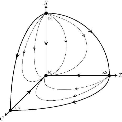
Figure 3: The compactified state space ($X$, $Z$, $C$) for the Bianchi V reduced system, including fixed points at infinity. These represent the isotropic singularity (IS), the Kasner anisotropic singularity (KS) and the curvature singularity (CS). (a) Left panel: The state space when $\alpha>-1$. (b) Right panel: the state space when $\alpha<-1$. It is clear that standard (non phantom) trajectories are asymptotic to the IS fixed point in the past.

The first two fixed points M and dS represent the Minkowski and generalized de Sitter points as in the Bianchi I case and retain the same stability character. The third point (CS) is the curvature singularity, which is curvature dominated ($C\to 1$, or $c\to\infty$). The fourth point (IS) represents the isotropic singularity and the final fixed point (KS) represents the anisotropic Kasner singularity. We now discuss the state space diagrams for this system. The case $\alpha>-1$ is shown in Fig. 3(a) (this corresponds to case A). The $X-Z$ plane ($C=0$) is the invariant manifold which represents the reduced and compactified Bianchi I state space, which is a manifold of the larger Bianchi V state space. The $Z-C$ plane ($X=0$) is the vacuum invariant manifold and the $X-C$ plane ($Z=0$) is the isotropic invariant manifold. The Minkowski point M is the future attractor for all trajectories in the region. The isotropic singularity (IS) is the generic past attractor, while the anisotropic Kasner singularity (KS) and curvature singularity (CS) have saddle stability character. As in the Bianchi I case, in general the past singularity is isotropic.

In the case $\alpha<-1$, depicted in Fig. 3(b), there are five fixed points, M, dS, CS, IS and KS. The state space is split into two regions by the separatrix manifold joining the points dS, CS and KS. This manifold is given by $X=X_{\Lambda}$, where:

$$X_{\Lambda} = \tau\sqrt{\frac{1-C^{2}-Z^{2}}{1+\tau^{2}}}.$$ (61)

and $\tau=-(\alpha+1)$. In the $Z-C$ plane ($X=0$, vacuum invariant manifold) the dynamics are unaffected by the change in $\alpha$. The $X-C$ plane ($Z=0$, isotropic invariant manifold) is divided into two regions by the separatrix. In the region above the separatrix ($X>X_{\Lambda}$, corresponding to case B) the fluid behaves in a standard manner. The IS fixed point has repeller stability character and all trajectories are asymptotic to it in the past. The dS fixed point is the generic future attractor. The CS and KS fixed points have saddle stability character in this region. In the region below the separatrix ($X<X_{\Lambda}$, corresponding to case C) the fluid behaves in a phantom manner. The KS fixed point is a repeller and the dS fixed point the attractor. The M and CS fixed points have saddle stability character. In general, trajectories are asymptotic to the Kasner singularity in the past and the generalized de Sitter model in the future.

IV Dynamics of anisotropy and inhomogeneity

We have seen in the previous section that generic trajectories of Bianchi I and V anisotropic models with standard (non-phantom) matter of type A and B asymptotically approach an isotropic singularity in the past, with the Hubble normalized shear vanishing, $\Sigma\rightarrow 0$. Since the Bianchi I and V models are rather special and homogeneous, we now want to see if this behavior is restricted to these models only, or if instead is stable against small generic inhomogeneuos perturbations. That is, we want to see if appropriately defined dimensionless quantities measuring the deviation from homogeneity in a covariant gauge invariant way decay to zero when the singularity is approached. Since we are only interested in the neighborhood of the singularity, we only need to consider perturbations of the spatially flat ($K=0$) homogenous and isotropic cosmological models (the flat Friedmann models, i.e. the vertical $X$ axis in Figs. 2 and 3) with quadratic EoS

$$P=\alpha\rho+\frac{\rho^{2}}{\rho_{c}}.$$ (62)

Given this EoS, $\rho+3P>0$ is always satisfied for high enough $\rho$, whatever $\alpha$ is, hence at high enough energies the background evolution is non-inflationary, $\ddot{a}<0$. Therefore we only need to consider large scale perturbations, i.e. scales much larger than the Hubble horizon $H^{-1}$, because for any given perturbation scale $\lambda$ there is always a time $t_{H}$ (the horizon crossing time) such that for $t\ll t_{H}$ we have $\lambda\gg H^{-1}$.

For simplicity we now focus on models of type A only, with $\alpha>-1$; it can be shown that similar results can be obtained in case B, $\alpha<-1$. For this case we re-write Eq. (8) as

$$\rho(a)=\frac{\rho_{c}(\alpha+1)}{(\frac{a}{a_{s}})^{3(\alpha+1)}-1},$$ (63)

where

$$a_{s}\equiv A^{\frac{1}{3(\alpha+1)}}$$ (64)

is the finite value of the scale factor such that the energy density has a pole like singularity. $A$ is a constant given by (6) and is expressed in terms of $\rho_{o}$, $a_{o}$, $\rho_{c}$ and $\alpha$. Given that the background is a spatially flat Friedmann model the Friedmann equation ($H^{2}=\rho/3$) gives directly the Hubble expansion scalar $H$, while $a_{o}$ can be fixed arbitrarily, a freedom that we will use later. The sound speed for the fluid is given by:

$$c_{s}^{2}=\frac{\partial P}{\partial\rho}=\alpha+\frac{2\rho}{\rho_{c}}.$$ (65)

The more commonly used EoS parameter $w$ is:

$$w=\frac{P}{\rho}=\alpha+\frac{\rho}{\rho_{c}}.$$ (66)

The sound speed and EoS variable are then related by the following relationship:

$$c_{s}^{2}=2w-\alpha.$$ (67)

Thus in case A our parameter $\alpha$ could be replaced by the combination $\alpha=2w-c_{s}^{2}$ of the more commonly used parameters $w$ and $c_{s}^{2}$.

IV.1 Dimensionless variables and harmonics

We use the covariant 1+3 approach  EB ; BDE ; VEE to study inhomogeneous and anisotropic gauge-invariant perturbations. In this approach, the information relating to inhomogeneous and anisotropic perturbations is contained in a set of (1+3) covariant variables. These variables are defined with respect to a preferred time-like observer congruence $u_{a}$. We use appropriate dimensionless density, expansion and curvature gradients which describe the scalar and vector parts of the corresponding perturbations:

$${\Delta}_{a} = \frac{a}{\rho}\nabla_{a}\rho,$$ (68)

$$Z_{a} = \frac{{\mathcal{Z}}_{a}}{H}=\frac{a}{H}\nabla_{a}H,$$ (69)

$${\mathcal{C}}_{a} = {a^{3}}\nabla_{a}{}^{(3)}{R}.$$ (70)

The dimensionless expansion normalized quantities for the shear $\sigma_{ab}$, the vorticity $\omega_{a}$, the electric $E_{ab}$ and magnetic $H_{ab}$ parts of the Weyl tensor are:

$$\Sigma_{ab}=\frac{\sigma_{ab}}{H}\;,~{}~{}W_{a}=\frac{\omega_{a}}{H}\;,~{}~{}{\cal E}_{ab}=\frac{E_{ab}}{H^{2}}\;,~{}~{}{\cal H}_{ab}=\frac{H_{ab}}{H^{2}}\;,$$ (71)

where $H$ is the Hubble scalar, $H=\dot{a}/a$. Here $\omega_{a}=\eta_{abc}\omega^{bc}$ is the usual vorticity vector. In order to calculate all the relevant tensor perturbations it is useful to define a set of variables corresponding to the curls of the standard quantities. The curl of a given quantity will be denoted by an over-bar.

$$\bar{\Sigma}_{ab}=\frac{1}{H}\textmd{curl}{\Sigma_{ab}}\;,~{}~{}\bar{{\cal E}}_{ab}=\frac{1}{H}\textmd{curl}{\cal E}_{ab}\;,~{}~{}\bar{\cal H}_{ab}=\frac{1}{H}\textmd{curl}{\cal H}_{ab}\;.$$ (72)

The harmonics defined in BDE are used to expand the above tensors $X_{a}\;,X_{ab}$ in terms of scalar (S), vector (V) and tensor (T) harmonics $Q$. This results in a covariant and gauge invariant splitting of the evolution and constraint equations for the above quantities into three sets of evolution and constraint equations for scalar, vector and tensor modes. The scalar, vector and tensor quantities can be split such that:

$$X = X^{S}Q^{S}$$ (73)

$$X_{a} = k^{-1}X^{S}Q_{a}^{S}+X^{V}Q_{a}^{V}$$ (74)

$$X_{ab} = k^{-2}X^{S}Q_{ab}^{S}+k^{-1}X^{V}Q_{ab}^{V}+X^{T}Q_{ab}^{T}\;.$$ (75)

As said above, we will carry out our analysis in the long-wavelength limit $\lambda\gg H^{-1}$, or $k^{2}/a^{2}H^{2}\ll 1$ ($\lambda=a/k$). This is analogous to dropping the Laplacian terms in the evolution and constraint equations.

Table 5: The large scale behavior of the scalar quantities. The constants of integration ($\Delta_{i}$) correspond to the two independent modes. The non-zero constants $B_{i}$, $Z_{i}$, $\mathcal{C}_{0}$, $\Sigma_{i}$ and ${\cal E}_{i}$ can all be expressed in terms of $\Delta_{1,2}$, $\rho_{c}$ and $\alpha$. The symbol $\Xi$ represents the generalized hypergeometric function given in Eq. (88). The third column gives the behavior of the perturbation at the singularity. The last column gives the approximate late time behavior of the perturbation. The limits are given under the assumption that $\alpha>-1$ and $\rho_{c}>0$.

Quantity	$X_{-}$ Mode	$X_{+}$ Mode	Limit($a\rightarrow a_{s}$)	Limit($a\gg a_{s}$)
$\Delta$	$\Delta_{1}\frac{\sqrt{\rho_{c}(\alpha+1)a^{3(\alpha+1)}-{1}}}{a^{3}}$	$\Delta_{2}\frac{[{\rho_{c}(\alpha+1)a^{3(\alpha+1)}-1}]}{a^{2}}\left(1+\frac{B_{1}}{a}\Xi\right)$	$0$, $0$	$a^{{3(\alpha-1)}/{2}}$, $a^{3\alpha+1}$
$Z$	$Z_{1}\frac{\sqrt{\rho_{c}(\alpha+1)a^{3(\alpha+1)}-{1}}}{a^{3}}$	$Z_{2}\frac{[{\rho_{c}(\alpha+1)a^{3(\alpha+1)}-1}]}{a^{2}}\left(1-\frac{B_{2}}{a}\Xi\right)$	$0$, $0$	$a^{{3(\alpha-1)}/{2}}$, $a^{3\alpha+1}$
$\mathcal{C}$	0	$\mathcal{C}_{0}$	$0$, $\mathcal{C}_{0}$	$0$, $\mathcal{C}_{0}$
$\Sigma$	$\Sigma_{1}\frac{\sqrt{\rho_{c}(\alpha+1)a^{3(\alpha+1)}-{1}}}{a^{3}}$	$\Sigma_{2}\frac{[{\rho_{c}(\alpha+1)a^{3(\alpha+1)}-{1}}]}{a^{2}}\left(1-\frac{B_{2}}{a}\Xi\right)$	$0$, $0$	$a^{{3(\alpha-1)}/{2}}$, $a^{3\alpha+1}$
${\cal E}$	${\cal E}_{1}\frac{\sqrt{\rho_{c}(\alpha+1)a^{3(\alpha+1)}-{1}}}{a^{3}}$	${\cal E}_{2}\frac{[{\rho_{c}(\alpha+1)a^{3(\alpha+1)}-1}]}{a^{2}}\left(1+\frac{B_{1}}{a}\Xi\right)$	$0$, $0$	$a^{{3(\alpha-1)}/{2}}$, $a^{3\alpha+1}$

IV.2 Scalar perturbations

The evolution and constraint equations are greatly simplified if we use the previously defined dimensionless time derivative:

$$(~{}~{})^{\prime}=\frac{1}{H}\frac{d}{dt}=a\frac{d}{da}.$$ (76)

The linearized evolution equations for scalar perturbations are:

$${\Delta}^{\prime} = 3w\Delta-\frac{(w+1)}{H}\mathcal{Z},$$ (77)

$${\mathcal{Z}}^{\prime} = -2\mathcal{Z}-\frac{3H}{2}\Delta,$$ (78)

$$E^{\prime} = -3E-\frac{3H}{2}(w+1)\sigma,$$ (79)

$$\sigma^{\prime} = -2\sigma-\frac{E}{H}.$$ (80)

The set of equations contain a mixture of Hubble normalized and non-normalized variables, however all solutions presented are appropriately normalized. In a addition we have a set of constraint equations for the scalar quantities:

$$\mathcal{C} = -4a^{2}H\mathcal{Z}+2a^{2}\rho\Delta,$$ (81)

$$3\Sigma = 2Z,$$ (82)

$${\cal E} = \Delta.$$ (83)

The system of equations is particularly difficult to solve in the above form. This is due to the form of $\rho(a)$, $H(a)$ and $w(a)$ (the pole like behavior at $a=a_{s}$). In order to solve the system of equations we carry out a change of variables. This is a parameter specific ($\rho_{c}$ and $\alpha$) non-linear transformation of the scale factor. Once the solutions are obtained, they are again expressed in terms of the original normalized scale factor $a$. The solutions to the system of equations can be split into modes which are sourced by the gradient of the 3-curvature ($\mathcal{C}$, which is constant in the long-wavelength limit) perturbation (subscript $+$) and those which are not (subscript $-$). The solutions for the scalar contribution to the density and expansion gradient’s are of the form:

$$\Delta_{-} = \Delta_{1}\frac{\sqrt{\rho_{c}(\alpha+1)a^{3(\alpha+1)}-{1}}}{a^{3}},$$ (84)

$$\Delta_{+} = \Delta_{2}\frac{[{\rho_{c}(\alpha+1)a^{3(\alpha+1)}-{1}}]}{a^{2}}\times\left(1+\frac{B_{1}}{a}\Xi\right),$$ (85)

$${Z}_{-} = {Z}_{1}\frac{\sqrt{\rho_{c}(\alpha+1)a^{3(\alpha+1)}-{1}}}{a^{3}},$$ (86)

$${Z}_{+} = {Z}_{2}\frac{[{\rho_{c}(\alpha+1)a^{3(\alpha+1)}-{1}}]}{a^{2}}\times\left(1-\frac{B_{2}}{a}\Xi\right).$$ (87)

The $\Delta_{i}$’s ($i=1,2$) are the arbitrary constants of integration and correspond to the two independent modes. The other constants $B_{i}$ and $Z_{i}$ can be expressed in terms of the arbitrary constants $\Delta_{i}$ and the EoS parameters $\rho_{c}$ and $\alpha$. The symbol $\Xi$ represents the generalized hypergeometric function and is of the form:

$$\Xi = {}_{2}{\mathcal{F}}_{1}\left(\left[\frac{1}{2},\frac{3\alpha+2}{3(\alpha+1)}\right],\left[\frac{3}{2}\right],1-b\right),$$ (88)

$$b = \rho_{c}(\alpha+1)a^{3(\alpha+1)}.$$ (89)

The generalized hypergeometric function is equal to unity at the singularity (${}_{2}{\mathcal{F}}_{1}([i,j],[k],0)=1$), where also $b=1$ after using the freedom in $a_{o}$ to set $A=[\rho_{c}(1+\alpha)]^{-1}$. In addition the quantity $(1\pm~{}B_{i}\Xi/a)\to 1$ as $a\gg a_{s}$, the hypergeometric function is a correction to the solutions at the singularity and plays a subdominant role at late times. The perturbations all decay as we approach the singularity in the past ($\Delta_{\pm}\to 0$ and $Z_{\pm}\to 0$ as $a\to a_{s}$). At late times ($a\gg a_{s}$) the various modes are approximately:

$$\Delta_{-} \approx \Delta_{1}a^{{3(\alpha-1)}/{2}},$$ (90)

$$\Delta_{+} \approx \Delta_{2}a^{3\alpha+1},$$ (91)

$${Z}_{-} \approx {Z}_{1}a^{{3(\alpha-1)}/{2}},$$ (92)

$${Z}_{+} \approx {Z}_{2}a^{3\alpha+1}.$$ (93)

This is the corresponding behavior one would expect for a fluid with a linear EoS. The modes asymptotically evolve as there linear EoS counterparts at late times. The perturbation modes for each of the scalar quantities can be found in Table 5. The constants of integration are the $\Delta_{i}$’s and all other constants ($Z_{i}$, $\Sigma_{i}$, $\mathcal{E}_{i}$, $B_{i}$ and $\mathcal{C}_{0}$ ) can be expressed in terms of these constants and the EoS parameters. The behavior of each mode is also given in the two limits, the first is at the singularity ($a\to a_{s}$) and the second is at late times ($a\gg a_{s}$). The limits are given assuming $\alpha>-1$ and $\rho_{c}>0$.

Table 6: The large scale behavior of the vector quantities. The constants of integration ($\Delta_{i}$ and $W_{1}$) correspond to the three independent modes. The non-zero constants $B_{i}$, $Z_{i}$, $\mathcal{C}_{0}$, $\mathcal{H}_{1}$, $\Sigma_{i}$ and ${\cal E}_{i}$ can all be expressed in terms of $\Delta_{1,2}$, $W_{1}$, $\rho_{c}$ and $\alpha$. See the caption of Table 5 for further details.

Quantity	$X_{-}$ Mode	$X_{+}$ Mode	Limit($a\rightarrow a_{s}$)	Limit($a\gg a_{s}$)
$\Delta$	$\Delta_{1}\frac{\sqrt{\rho_{c}(\alpha+1)a^{3(\alpha+1)}-{1}}}{a^{3}}$	$\Delta_{2}\frac{[{\rho_{c}(\alpha+1)a^{3(\alpha+1)}-1}]}{a^{2}}\left(1+\frac{B_{1}}{a}\Xi\right)$	$0$, $0$	$a^{{3(\alpha-1)}/{2}}$, $a^{3\alpha+1}$
$Z$	$Z_{1}\frac{\sqrt{\rho_{c}(\alpha+1)a^{3(\alpha+1)}-{1}}}{a^{3}}$	$Z_{2}\frac{[{\rho_{c}(\alpha+1)a^{3(\alpha+1)}-1}]}{a^{2}}\left(1-\frac{B_{2}}{a}\Xi\right)$	$0$, $0$	$a^{{3(\alpha-1)}/{2}}$, $a^{3\alpha+1}$
$\mathcal{C}$	0	$\mathcal{C}_{0}$	$0$, $\mathcal{C}_{0}$	$0$, $\mathcal{C}_{0}$
$W$	$W_{1}\frac{[\rho_{c}(\alpha+1)a^{3(\alpha+1)}-{1}]^{{5}/{2}}}{a^{3\alpha+8}}$	$-$	$0$	$a^{{(9\alpha-1)}/{2}}$
$\mathcal{H}$	$\mathcal{H}_{1}\frac{[{\rho_{c}(\alpha+1)a^{3(\alpha+1)}-{1}}]}{a^{4}}$	$-$	$0$	$a^{{3(\alpha-1)}}$
$\Sigma$	$\Sigma_{1}\frac{\sqrt{\rho_{c}(\alpha+1)a^{3(\alpha+1)}-{1}}}{a^{3}}$	$\Sigma_{2}\frac{[{\rho_{c}(\alpha+1)a^{3(\alpha+1)}-{1}}]}{a^{2}}\left(1-\frac{B_{2}}{a}\Xi\right)$	$0$, $0$	$a^{{3(\alpha-1)}/{2}}$, $a^{3\alpha+1}$
${\cal E}$	${\cal E}_{1}\frac{\sqrt{\rho_{c}(\alpha+1)a^{3(\alpha+1)}-{1}}}{a^{3}}$	${\cal E}_{2}\frac{[{\rho_{c}(\alpha+1)a^{3(\alpha+1)}-1}]}{a^{2}}\left(1+\frac{B_{1}}{a}\Xi\right)$	$0$, $0$	$a^{{3(\alpha-1)}/{2}}$, $a^{3\alpha+1}$

IV.3 Vector perturbations

The linearized evolution equations for the vector components of the perturbations in the large-scale limit are:

$${\Delta}^{\prime} = 3w\Delta-\frac{(w+1)}{H}\mathcal{Z},$$ (94)

$${\mathcal{Z}}^{\prime} = -2\mathcal{Z}-\frac{3H}{2}\Delta,$$ (95)

$$\omega^{\prime} = (3c_{s}^{2}-2)\omega,$$ (96)

$$E^{\prime} = -3E-\frac{3H}{2}(w+1)\sigma,$$ (97)

$$\sigma^{\prime} = -2\sigma-\frac{E}{H}.$$ (98)

The constraint equations for the vector variables are

$$\mathcal{C} = -4a^{2}H\mathcal{Z}+2a^{2}\rho\Delta,$$ (99)

$${\cal H} = \frac{3a}{2}(w+1)HW,$$ (100)

$$3\Sigma = 2Z,$$ (101)

$${\cal E} = \Delta.$$ (102)

The perturbation modes for each of the vector quantities can be found in Table 6. The constants of integration ($\Delta_{i}$ and $W_{1}$) correspond to the three independent modes. The non-zero constants $B_{i}$, $Z_{i}$, $\mathcal{C}_{0}$, $\mathcal{H}_{1}$, $\Sigma_{i}$ and ${\cal E}_{i}$ can all be expressed in terms of the constants of integration and the EoS parameters. The last two columns give the behavior of the perturbation in the two limits. As in the case of the scalar contributions all perturbations decay at the singularity and asymptotically approach the standard linear EoS behavior at late times.

Table 7: The large scale behavior of the tensor quantities. The constants of integration ($\Sigma_{i}$ and $\mathcal{H}_{i}$) correspond to the four independent modes. The non-zero constants $B_{i}$, $\mathcal{E}_{i}$, $\bar{{\cal E}}_{i}$ and $\bar{\Sigma}_{i}$ can all be expressed in terms of $\Sigma_{1,2}$, $\mathcal{H}_{1,2}$, $\rho_{c}$ and $\alpha$. See the caption of Table 5 for further details.

Quantity	$X_{-}$ Mode	$X_{+}$ Mode	Limit($a\rightarrow a_{s}$)	Limit($a\gg a_{s}$)
$\Sigma$	$\Sigma_{1}\frac{\sqrt{\rho_{c}(\alpha+1)a^{3(\alpha+1)}-{1}}}{a^{3}}$	$\Sigma_{2}\frac{[{\rho_{c}(\alpha+1)a^{3(\alpha+1)}-{1}}]}{a^{2}}\left(1-\frac{B_{2}}{a}\Xi\right)$	$0$, $0$	$a^{{3(\alpha-1)}/{2}}$, $a^{3\alpha+1}$
${\cal E}$	${\cal E}_{1}\frac{\sqrt{\rho_{c}(\alpha+1)a^{3(\alpha+1)}-{1}}}{a^{3}}$	${\cal E}_{2}\frac{[{\rho_{c}(\alpha+1)a^{3(\alpha+1)}-1}]}{a^{2}}\left(1+\frac{B_{1}}{a}\Xi\right)$	$0$, $0$	$a^{{3(\alpha-1)}/{2}}$, $a^{3\alpha+1}$
${\cal H}$	${\cal H}_{1}\frac{[{\rho_{c}(\alpha+1)a^{3(\alpha+1)}-1}]}{a^{4}}$	${\cal H}_{2}\frac{{[{\rho_{c}(\alpha+1)a^{3(\alpha+1)}-1}]}^{\frac{3}{2}}}{a^{3}}\left(1-\frac{B_{3}}{a}\Xi\right)$	$0$, $0$	$a^{{3\alpha-1}}$, $a^{3(3\alpha+1)/2}$
$\bar{{\cal E}}$	$\bar{{\cal E}}_{1}\frac{[{\rho_{c}(\alpha+1)a^{3(\alpha+1)}-1}]}{a^{4}}$	$\bar{{\cal E}}_{2}\frac{{[{\rho_{c}(\alpha+1)a^{3(\alpha+1)}-1}]}^{\frac{3}{2}}}{a^{3}}\left(1+\frac{B_{4}}{a}\Xi\right)$	$0$, $0$	$a^{{3\alpha-1}}$, $a^{3(3\alpha+1)/2}$
$\bar{\Sigma}$	$\bar{\Sigma}_{1}\frac{[{\rho_{c}(\alpha+1)a^{3(\alpha+1)}-1}]}{a^{4}}$	$\bar{\Sigma}_{2}\frac{{[{\rho_{c}(\alpha+1)a^{3(\alpha+1)}-1}]}^{\frac{3}{2}}}{a^{3}}\left(1-\frac{B_{3}}{a}\Xi\right)$	$0$, $0$	$a^{{3\alpha-1}}$, $a^{3(3\alpha+1)/2}$
$\bar{{\cal H}}$	$0$	$0$	$-$	$-$

IV.4 Tensor perturbations

The linearized evolution equations for the tensor components of the perturbations in the large-scale limit are:

$$E^{\prime} = -3E-\frac{3H}{2}(w+1)\sigma,$$ (103)

$$\sigma^{\prime} = -2\sigma-\frac{E}{H},$$ (104)

$${\cal H}^{\prime} = -3{\cal H}-\frac{1}{H}\bar{E}$$ (105)

$$\bar{E}^{\prime} = -3\bar{E}-\frac{3H}{2}(w+1){\cal H}.$$ (106)

The constraint equations for the tensor variables are

$$\cal{H} = \bar{\Sigma},$$ (107)

$$\bar{{\cal H}} = 0.$$ (108)

The perturbation modes for each of the tensor quantities can be found in Table 7. The constants of integration ($\Sigma_{i}$ and $\mathcal{H}_{i}$) correspond to the four independent modes. The non-zero constants $B_{i}$, $\mathcal{E}_{i}$, $\bar{{\cal E}}_{i}$ and $\bar{\Sigma}_{i}$ can all be expressed in terms of the constants of integration and the EoS parameters. The perturbations all decay at the singularity and evolve as there linear EoS counterparts at late times.

V Conclusions

In this paper we have investigated the effects of a quadratic EoS in homogenous and inhomogeneous anisotropic cosmological models in general relativity, in order to understand if in this context the quadratic EoS can isotropize the universe at early times, when the initial singularity is approached.

The first motivation for this work is that in the context of brane world cosmological models the term quadratic in the energy density that appears in the effective 4-dimensional equations of motion on the brane dominates at early times, driving the evolution to an initial isotropic singularity under reasonable assumptions. Therefore, under these assumptions, in the brane world scenario we do not have the classical isotropy problem: the isotropy we observe today is built in, that is it follows from generic initial conditions. This is at odds with the classical and now widely accepted results in general relativity BKL ; LL ; Ashtekar , where general cosmological models with a linear EoS are highly anisotropic in the past, approaching the singularity a-la BKL, i.e. with mixmaster dynamics, so that in general one needs special initial conditions to have isotropy at late times, even to initiate an inflationary phase KT .

Secondly, we also wanted to study the effects at early times and at high energies of the same type of EoS used in Paper I AB , relaxing the symmetries assumed there. The focus in Paper I AB was on the possible use of a quadratic EoS as an effective way of representing a dark energy component or unified dark matter in the context of homogeneous isotropic models of relevance for the universe at late times. Here we have used the simplified EoS $P=\alpha\rho+\rho^{2}/\rho_{c}$, which still allows for an effective cosmological constant and phantom behavior, and is general enough to analyze the dynamics at high energies.

In summary, our aim here was to investigate if the behavior of the anisotropy at the singularity found in the brane scenario is recreated in the general relativistic context if we consider a quadratic term in the EoS. That is to say, in the language of dynamical system theory, do we have a scenario where the generic asymptotic past attractor in general relativity is an isotropic model, thanks to a non-linear (specifically, quadratic) EoS.

To this end, we have first summarized in Section II the classification of the energy density evolution in three classes, A, B and C, following from the energy conservation for the EoS $P=\alpha\rho+\rho^{2}/\rho_{c}$ (a broader classification can be found in Section II of Paper I AB ). In Section III, using dynamical system methods WE ; AP , we have studied the Bianchi I and V cosmological models with a fluid with this EoS. We first considered the case when $\alpha>-1$ (case A). The physically interesting quantity $\Sigma$, the Hubble normalized dimensionless measure of shear, describes the anisotropy. In the expanding Bianchi I and V models this quantity always decreases at late times, as in the case with a linear EoS, approaching a Minkowski model. However, we can now have stages at early times in which $\Sigma$ grows, vanishing at the initial singularity, and generic trajectories in the compactified state space asymptotically approach in the past the isotropic fixed point IS, as depicted in Figs. 2 and 3. This behavior is similar to the quasi-isotropic expansion seen in the anisotropic brane-world models, but occurs for different reasons. The quasi-isotropic expansion is caused by the fact that the EoS becomes “super-stiff” at early times but decreases to finite values at late times. At the initial singularity (which is of Type III, see NOT ; barrow ) the anisotropy is always sub-dominant and we recover the standard linear EoS behavior at late times. In the case $\alpha<-1$, the state space can be divided in two regions. In the standard fluid region ($X>X_{\Lambda}$, case B) the behavior at early times is similar to the $\alpha>-1$ case, with generic trajectories in the compactified state space approaching the isotropic fixed point IS of Figs. 2 and 3. At late times instead trajectories asymptotically approach generalized expanding de Sitter models. Finally, in the phantom fluid region ($X<X_{\Lambda}$, case C) the anisotropy dominates at early times and the past singularity is anisotropic. Trajectories are asymptotic to the expanding de Sitter model at late times.

The submanifold $\Sigma=0$ in the state space for the Bianchi models represents homogeneous isotropic spatially flat Friedmann-Robertson-Walker models, with IS as past attractor. In order to see if IS can be regarded as the past attractor of a larger class of general models with no symmetries, we have studied in Section IV, using covariant and gauge invariant variables EB ; BDE ; VEE , the first order inhomogeneous anisotropic perturbations of these flat isotropic models, focusing on those of class A. The linearized equations have been solved in the large scale limit $\lambda\gg H^{-1}$, neglecting the Laplacian operators terms. As explained in Section I, only perturbations larger then the Hubble horizon $H^{-1}$ are relevant in our analysis. The main results of this section are given in Table’s 5, 6 and  7. The tables contain the form of the solutions and asymptotic behavior of the physically relevant quantities for both early ($a\to a_{s}$) and late times ($a\gg a_{s}$). The quantities have been harmonically decomposed into the standard scalar, vector and tensor components. These include the expansion normalized vorticity, shear, and electric and magnetic contributions of the Weyl tensor. In addition, we consider the gradients of the energy density, expansion and three-curvature. As expected, at late times the perturbations evolve as if the fluid obeyed a linear EoS, i.e. the standard behavior is recovered in this limit. The evolution of the perturbations at early times is our main result. Indeed, we find that all perturbations tend to zero near the singularity. Thus a perturbed quasi-isotropic model with generic initial condition evolves from the isotropic past attractor IS. This indicates that in general relativity with matter described by a non-linear EoS there are general cosmological models, corresponding to a non zero measure subset of all possible generic initial conditions LL , that isotropize as the initial singularity is approached, with IS as the past attractor. As for the brane models, this would be at odds with the standard BKL results BKL ; LL ; Ashtekar .

Singularities are commonly regarded as signaling the failure of classical gravitational theories, requiring a quantum theory of gravity to deal with trans-Plankian energies. Even in effective theories, perhaps cosmology doesn’t require them, as in the pre-big-bang scenario pbb . In any case, it is important to understand which is the typical classical dynamical behavior in the neighborhood of singularities, as this possibly signals what the generic outcome of a quantum theory should be at low (sub-Plankian) energies. In the BKL picture for fluids with linear EoS and other simple type of matter Ashtekar this behavior is mixmaster and the effects of matter become negligible close to the singularity: we may say that effectively in this limit the space-time still tells matter how to move, but matter is no longer able to tell the space-time how to curve. Perhaps this behavior should be regarded as pathological, and peculiar of the energy-momentum tensor of linear EoS matter (or other simple energy-momentum tensor) in general relativity. In practice we know close to nothing about matter fields at the highest (close to Plankian) cosmological energies, and these may require a non-linear effective EoS description in general, or maybe Einstein equations with an effective non-linear EoS are the Einstein frame version of some effective low energy (sub-Plankian) theory. In both cases, our analysis of Einstein equations with a fluid with a quadratic EoS indicates that the typical initial state is isotropic. The singularity is matter dominated, and of a type that could admit an extension. Interestingly, the EoS considered here are a subclass of those used in Paper I AB to model a dark energy component or unified dark matter, allowing for effective cosmological constants.

- (1) K. Ananda, M. Bruni, Cosmo-dynamics and dark energy with non-linear equation of state: a quadratic model, Phys. Rev. D, submitted. arXiv:astro-ph/0512224
- (2) R. Scranton et al. [SDSS Collaboration], arXiv:astro-ph/0307335; M. Tegmark et al. [SDSS Collaboration], Phys. Rev. D 69, 103501 (2004) [arXiv:astro-ph/0310723].
- (3) C. L. Bennett et al., Astrophys. J. Suppl. 148, 1 (2003) [arXiv:astro-ph/0302207]; L. Page et al., Astrophys. J. Suppl. 148, 233 (2003) [arXiv:astro-ph/0302220].
- (4) D. N. Spergel et al. [WMAP Collaboration], Astrophys. J. Suppl. 148, 175 (2003) [arXiv:astro-ph/0302209].
- (5) D. N. Spergel et al. [WMAP Collaboration], [arXiv:astro-ph/0603449].
- (6) C.B. Collins, S.W. Hawking, Astrophys. J. Suppl. 180, 317 (1973).
- (7) D. Eardley, E. Liang and R. Sachs, J. Math. Phys. 13, 99 (1972).
- (8) R. W. Wald, Phys. Rev. D 28, 2118 (1983).
- (9) E. W. Kolb and M. S. Turner, The Early Universe (Westview Press, Oxford, 1990).
- (10) M. Bruni, S. Matarrese annd O. Pantano, Phys. Rev. Lett., 74, 1916–1919 (1995).
- (11) D. Garfinkle, Phys. Rev. Lett. 93, 161101 (2004); Int. J. Mod. Phys. D13 (2004). 2261-2266
- (12) V. A. Belinski, E. M. Lifschitz and I. M. Khalatnikov, Adv. Phys. 19, 525 (1970); V. A. Belinski, E. M. Lifschitz and I. M. Khalatnikov, Adv. Phys. 31, 639 (1982).
- (13) L. D. Landau and E. M. Lifshitz, The Classical Theory of Fields (Pergamon, Oxford 1975).
- (14) For reviews on singularities in general relativity and other theories of gravity see the articles of Rendall and Nicolai in 100 Years of Relativity. Space-Time Structure: Einstein and Beyond, ed. by A. Ahtekar (World Scientific, 2005).
- (15) T. Shiromizu, K. i. Maeda and M. Sasaki, Phys. Rev. D 62, 024012 (2000) [arXiv:gr-qc/9910076].
- (16) H. A. Bridgman, K. A. Malik and D. Wands, Phys. Rev. D 65, 043502 (2002) [arXiv:astro-ph/0107245].
- (17) D. Langlois, Astrophys. Space Sci. 283, 469 (2003) [arXiv:astro-ph/0301022].
- (18) R. Maartens, Living Rev. Rel. 7, 7 (2004) [arXiv:gr-qc/0312059].
- (19) R. Maartens, V. Sahni and T. D. Saini, Phys. Rev. D 63, 063509 (2001) [arXiv:gr-qc/0011105].
- (20) A. Campos and C. F. Sopuerta, Phys. Rev. D 63, 104012 (2001) [arXiv:hep-th/0101060].
- (21) A. A. Coley, Phys. Rev. D 66, 023512 (2002) [arXiv:hep-th/0110049].
- (22) R. J. van den Hoogen, A. A. Coley and Y. He, Phys. Rev. D 68, 023502 (2003) [arXiv:gr-qc/0212094].
- (23) A. A. Coley, Y. He and W. C. Lim, Class. Quant. Grav. 21, 1311 (2004) [arXiv:gr-qc/0312075].
- (24) P. Dunsby, N. Goheer, M. Bruni and A. Coley, Phys. Rev. D 69, 101303 (2004) [arXiv:hep-th/0312174].
- (25) N. Goheer, P. K. S. Dunsby, A. Coley and M. Bruni, Phys. Rev. D 70, 123517 (2004) [arXiv:hep-th/0408092].
- (26) J. Wainwright and G. F. R. Ellis, Dynamical systems in cosmology (Cambridge University Press, Cambridge, 1997).
- (27) D. K. Arrowsmith and C. M. Place, Dynamical systems: differential equations, maps and chaotic behaviour (Chapman and Hall, London, 1992).
- (28) G. F. R. Ellis and M. Bruni, Phys. Rev. D 40, 1804 (1989).
- (29) M. Bruni, P. K. S. Dunsby and G. F. R. Ellis, Astrophys. J. 395, 34 (1992).
- (30) For a review, see, G.F.R. Ellis, H. van Elst, in Theoretical and Observational Cosmology, ed. M. Lachi‘eze-Rey (Kluwer, Dordrecht, 1999), arXiv:gr-qc/9812046.
- (31) R. R. Caldwell, Phys. Lett. B 545, 23-29 (2002).
- (32) S. Nojiri, S. D. Odintsov and S. Tsujikawa, Phys. Rev. D 71, 063004 (2005) [arXiv:hep-th/0501025].
- (33) J. D. Barrow, Class. Quant. Grav. 21, 5619 (2004) [arXiv:gr-qc/0409062]; J. D. Barrow, Class. Quant. Grav. 21, L79 (2004) [arXiv:gr-qc/0403084].
- (34) G. Veneziano, Lectures delivered in Les Houches, July 1999, [arXiv:hep-th/0002094].