Global visibility of naked singularities

Abstract.

Global visibility of naked singularities is analyzed here for a class of spherically symmetric spacetimes, extending previous studies - limited to inhomogeneous dust cloud collapse - to more physical valid situations in which pressures are non-vanishing. Existence of nonradial geodesics escaping from the singularity is shown, and the observability of the singularity from far-away observers is discussed.

1. Introduction

The study of gravitational collapse of spherically symmetric solutions in General Relativity led to many examples of locally naked singularities, starting from pioneering works in the early 80’s – a quite exhaustive and updated list of references can be found in reviews [8, 10]. Most of these papers concentrate on the aim to find photons emanated from the singularity and escaping the Schwarzschildian trapped region at least locally. Moreover, the analysis has been always limited to the study of radial null geodesics, quite simplifying then the system to study, which remains not defined at the singular point, but fully decouples.

However, in order to study the effects of these photons for a distant observer, global behavior of null geodesics must be studied in full generality, since nonradial geodesics, with nonzero angular momentum, determine the angular diameter of the central naked singularity as seen by the observers, giving the measure of the ”size” of the singularity. In this direction there are in literature quite detailed studies of Tolman–Bondi self similar dust cloud collapse. In [2, 12] necessary conditions – which actually turn out to be sufficient – for nonradial geodesics existence are derived, and behavior at infinity of these photons is numerically studied for some particular case. Further, a complete result of nonradial geodesic existence but under the assumption of self similarity of the dust solution is fully proved in [14], and considerations about topology of the singularity are derived.

Of course, the dust model cannot be considered as a good physical model of singularity formation, because pressures are expected to occur during the collapse. In this paper we extend the results on dust models to a wide class of solutions, found in [7], for which local nakedness results from a suitable choice of initial data. This class represents the wider set found so far of locally naked singularities in the gravitational collapse of elastic materials. Since these models are not pressureless, and in particular radial pressure does not generally vanish along a timelike hypersurface, a junction between a solution from this class and a anisotropic generalization of de Sitter space time discussed in [5] is performed to construct a global model. It is found that properties satisfied by dust solution and showed in previously cited works remains qualitatively valid for this wider class of collapsing spacetimes.

The paper is organized as follows. Interior and exterior solutions are described in Section 2, and local existence of nonradial geodesic – which are continued in the exterior spacetime using junction conditions – is derived in Section 3. The resulting behavior for a distant observer is analyzed in Section 4, together with some remarks about photons with infinite redshift. Last Section 5 is devoted to overall conclusions.

2. Collapse of spherical anisotropic matter

In this part we briefly review the model we will deal with for the rest of the paper. The spacetime will be made by two different solutions to Einstein field equations: an interior part, that collapses until singularity forms, and an exterior part, that is matched with the former at a timelike hypersurface in order to satisfy Israel–Darmois conditions [9]; it amounts to say that both first and second fundamental forms induced by the two solutions on this hypersurface respectively coincide. The interior part is described by the collapsing anisotropic solutions found in [7], which will be matched with the de Sitter generalizations discussed in [5] (see also references therein).

2.1. Interior region

The interior region is provided by a class of anisotropic collapsing matter. To describe it, the use of area–radius coordinates, first introduced by Ori [15], turns out to be more useful than usual comoving reference frame

(2.1) $$\text{d}s^{2}=-e^{2\nu}\text{d}t^{2}+\frac{1}{\eta}\text{d}r^{2}+R^{2}(\text{d}\theta^{2}+\sin^{2}\theta\,\text{d}\varphi^{2}).$$

Indeed, as well known [11], the general spherical matter distribution can be given assigning energy density $\epsilon$ and pressures $p_{r}$ and $p_{t}$ as suitable functions of the triple $(r,R,\eta)$. Under the assumption $\frac{\partial p_{r}}{\partial\eta}=0$, in [7] it is shown that the metric takes the form

(2.2a) $$\text{d}s^{2}=-A(r,R)\text{d}r^{2}-2B(r,R)\text{d}R\text{d}r-C(r,R)\text{d}R^{2}+R^{2}(\text{d}\theta^{2}+\sin^{2}\theta\,\text{d}\varphi^{2}),$$

where

(2.2b) $$A=\left(1-\frac{2\Psi}{R}\right)G^{2},\quad B=-G\,\frac{Y}{u},\quad C=\frac{1}{u^{2}}.$$

In (2.2b), the two functions $$\Psi(r,R) Y(r,R)$$ and are arbitrary (positive) functions while

(2.2c) $$u^{2}=Y^{2}+\frac{2\Psi}{R}-1,$$

and the function $$G$$ is given in terms of a quadrature:

(2.2d) $$G(r,R)=\int_{R}^{r}\frac{1}{Y(r,\sigma)}\frac{\partial(1/u)}{\partial r}(r,\sigma)\,\text{d}\sigma+\frac{1}{Y(r,r)u(r,r)}.$$

In particular, the function $\Psi$ represents Misner–Sharp mass. Conditions on Taylor developments of the above quantities may be given to characterize complete collapse and naked singularity formation, that we summarize in the following theorem.

Theorem 2.1 ([7]).

1. In the spacetime described by the metric (2.2a)–(2.2d), the singularity forms at the centre $r=0$ in a finite amount of comoving time if Taylor development of the function $Ru^{2}$ is as follows:

   (2.3) $$Ru^{2}=\alpha r^{3}+\beta r^{2}R+\gamma rR^{2}+\delta R^{3}+o(r^{2}+R^{2})^{3/2},\qquad(\alpha>0).$$

2. Under the above condition, and introduced the Taylor development of the (regular) function $G(r,0)$

   (2.4) $$G(r,0)=\xi r^{n-1}+o(r^{n-1}),$$

   then the central singularity is (locally) naked if, $n=1$, $n=2$, or $n=3$ and $\xi>\alpha\,\omega_{\mathrm{crit}}$ where $\omega_{\mathrm{crit}}=\frac{26+15\sqrt{3}}{2}$.

We also remark that this model possesses nonvanishing anisotropic pressures, which are given by [7]

(2.5) $$p_{r}=-\frac{1}{4\pi R^{2}}\frac{\partial\Psi}{\partial R},$$

(2.6) $$p_{t}=-\frac{1}{8\pi u\,R\,G}\left(\frac{1}{Y}\frac{\partial{}^{2}\Psi}{\partial r\partial R}-\frac{1}{Y^{2}}\frac{\partial\Psi}{\partial r}\frac{\partial Y}{\partial R}+u\,G\frac{\partial{}^{2}\Psi}{\partial R^{2}}\right),$$

and in this sense the model can be considered physically more reasonable than Tolman–Bondi dust collapsing sphere, where the spacetime is ruled by the pressureless equation of state $p_{r}=p_{t}=0$.

2.2. Exterior region

In our model, since the internal source is given by (2.2a), one cannot hope, in general, that radial pressure vanishes at some timelike hypersurface $\Sigma=\{(t,r,\theta,\phi)\,:\,r=r_{b}\}$. This is a quite restrictive feature of dust cloud collapsing model [13] or also non vanishing radial pressure models [11], that here arise only as very special cases, that happen when $\Psi=\Psi(r)$. Therefore, it cannot be possible to consider Schwarzschild vacuum solution as external region, if we want Israel–Darmois condition to be satisfied.

Hence, we perform a junction between the internal source satisfying conditions stated in Theorem 2.1, and the anisotropic generalization of de Sitter spacetime, which are a class of spherically symmetric solutions of Einstein equation satisfying the condition $\epsilon+p_{r}=0$ and admitting a particular $G_{4}$ group of motions (see [5]). A coordinate transformation exists, that brings the line element in the form

(2.7) $$\text{d}s^{2}=-\chi(R)\,\text{d}T^{2}+\chi(R)^{-1}\,\text{d}R^{2}+R^{2}\,\text{d}\Omega^{2},\quad\chi(R)=1-\frac{2M(R)}{R},$$

thereby obtaining a family of solutions as Misner–Sharp mass $M(R)$ varies. In [6] it is shown that, actually, any spherically symmetric line element (2.1) can be matched with a metric of this family at a timelike hypersurface $\Sigma$ as before, under the condition of continuity of mass only. Therefore, it suffices to choose

$$M(R)=\Psi(r_{b},R),\qquad\forall R\in[0,r_{b}]$$

and junction conditions will be certainly satisfied for all (comoving) times $t\geq 0$. The value of the external mass for bigger values of $R$ depends on the internal spacetime at comoving times prior to observation starting, and we will suppose that it is chosen such that

(2.8) $$\limsup_{R\to+\infty}M(R)<+\infty.$$

2.3. Energy condition

In order to deal with a physically reasonable class of solutions, we impose the weak energy condition (w.e.c.) on the energy–momentum tensor $T$ of the spacetime. Basically, this means $T(v,v)\geq 0$ for all timelike vectors $v$, and it is easily seen [7] that it holds in the internal region if, for each $r\in[0,r_{b}]$, the two functions of the variable $R$ only

(2.9) $$R\mapsto\frac{1}{Y(r,R)}\frac{\partial\Psi}{\partial r}(r,R),\qquad R\mapsto\frac{\partial\Psi}{\partial R}(r,R)$$

are nonnegative subsolutions of the same ODE:

(2.10) $$\frac{\mathrm{d}F}{\mathrm{d}R}\leq\frac{2}{R}\,F(R)$$

for $R>0$. In particular, for $r=r_{b}$, the above condition ensures w.e.c in the external region also (see [6, eq. (4.6)]).

Models of internal solutions satisfying (2.3), (2.8) and w.e.c. can be easily found: for instance, the choice

(2.11) $$\Psi(r,R)=\int_{0}^{r}\gamma(s)s^{2}\,\mathrm{d}s+\int_{0}^{R}\chi(\sigma)\sigma^{2}\,\mathrm{d}\sigma,\qquad Y=Y(r),$$

with $\gamma(s)$ and $\chi(\sigma)$ positive and not increasing in $[0,+\infty)$, allows for (2.3) and the weak energy condition to be satisfied. As an example, one may take

$$\chi(\sigma)=\frac{1}{(1+R^{3})^{4}}$$

in order to satisfy also (2.8). Note that, with the choice of $\chi=\mathrm{constant}$, the spacetime coincides with the so-called Tolman -Bondi -de Sitter (TBdS), and that’s the reason why, in [7], the models arising from the above choice (2.11) are termed anisotropysations of TBdS spacetime.

3. Null geodesics from the singularity

3.1. Geodesic equations

As stated in Theorem 2.1, conditions on the metric functions allow to determine when the central singularity is locally naked. This is made by showing the existence of a future pointing radial null geodesic which lies in the region $R>2\Psi$ and may be traced back to the central singularity. In [7] it is shown that, to obtain violations of cosmic censorship in spherical symmetry, one may restrict oneself in looking for null geodesic which are radial only. In other words, if a singularity is radially censored, it is censored all the way. Nevertheless, if one wants to study visibility under a more general point of view, also non radial light rays should be taken into account.

Let $\kappa$ be the affine parameter of the null geodesic. Without loss of generality, we will suppose that the geodesic lies in the hypersurface $\theta=\frac{\pi}{2}$, and then the angular components of tangent vector along the geodesic read

(3.1) $$\kappa^{\theta}:=\frac{\mathrm{d}\theta}{\mathrm{d}\kappa}=0,\qquad\kappa^{\phi}:=\frac{\mathrm{d}\phi}{\mathrm{d}\kappa}=\frac{\ell}{R^{2}},$$

where $\ell$ is the (conserved) angular momentum. Let us also introduce a function $q$ such that

(3.2) $$\kappa^{r}:=\frac{\mathrm{d}r}{\mathrm{d}\kappa}=\frac{1}{q\,R\,G}.$$

Then, expressing $R$, $\theta$ and $\phi$ as functions of $r$ instead of $\kappa$, the equations for null geodesics can be given in the following form:

(3.3a) $$\frac{\mathrm{d}R}{\mathrm{d}r}=u\,G\left[Y-u\sqrt{1+\left(\frac{\ell\,q}{u}\right)^{2}}\right],$$

(3.3b) $$\frac{\mathrm{d}\theta}{\mathrm{d}r}=0,\quad\frac{\mathrm{d}\phi}{\mathrm{d}r}=\frac{\ell\,q\,G}{R},$$

and

(3.3c) $$-\frac{1}{q}\frac{\mathrm{d}q}{\mathrm{d}r}-\frac{1}{G}\frac{\mathrm{d}G}{\mathrm{d}r}-\frac{1}{R}\frac{\mathrm{d}R}{\mathrm{d}r}-\frac{C\,A_{,r}+B(A_{,R}-2B_{,r})}{2G^{2}}\\ -\frac{C\,A_{,R}-B\,C_{,r}}{G^{2}}\frac{\mathrm{d}R}{\mathrm{d}r}+\frac{B\,C_{,R}+C(C_{,r}-2B_{,R})}{2G^{2}}\left(\frac{\mathrm{d}R}{\mathrm{d}r}\right)^{2}+\ell^{2}\frac{q^{2}\,B}{R}=0,$$

and $A,B,C$ are given in (2.2b). Dealing with radial geodesics results in vanishing of $\ell$, and so (3.3a), which is found imposing that the geodesic is null, becomes an ODE in the $R$ function only, which is enough to study at least the existence of corresponding pregeodesics. On the other side, when $\ell\neq 0$, also (3.3c) must be studied.

Before to state and show results, we restrict the analysis hereafter to the case when $n$ in (2.4) is equal to 3. As it will be cleared in Remark 3.4, this particular situation – that, as seen in the statement of Theorem 2.1, has a sort of “endstate transition” – corresponds to a so–called strong curvature singularity, unlike $n=1,2$ cases – at least along null radial geodesics. We refer the reader to Remark 3.4 below and, for instance, to [1, 17, 18] for a general insight about strong curvature conditions.

3.2. Null geodesics existence

Existence of null radial geodesics has already been proved in [7], using comparison arguments in ODE. We here complete the analysis about the asymptotic behavior of the geodesics finding also an existence result for nonradial geodesics.

Remark 3.1.

In the forthcoming Proposition it will be shown that the null geodesic equation can be put in the form

(3.4) $$\frac{\mathrm{d}y}{\mathrm{d}r}=\frac{1}{r}f(y)+g(r,y),$$

where $y(r)\in\mathds{R}^{n}$ and $f:\mathds{R}^{n}\to\mathds{R}$, $g:\mathds{R}^{n+1}\to\mathds{R}$ are $C^{1}$ functions; Introducing a new independent variable $s$ such that $\frac{\mathrm{d}r}{\mathrm{d}s}=-r(s)$ then, from (3.4), we obtain the system

(3.5) $$\begin{cases}&\frac{\mathrm{d}y}{\mathrm{d}s}=-f(y(s))-r(s)\,g(r(s),y(s)),\\ &\frac{\mathrm{d}r}{\mathrm{d}s}=-r(s),\end{cases}$$

whose solutions describe parameterizations of solutions of (3.4) by the parameter $s$. Equilibria of the above system (as $s\to+\infty$) are given by points $(y_{0},0)$ where $y_{0}$ is a root of $f(y)=0$, and searching for these equilibria amounts to search for admissible solutions of the so–called root equation, first introduced in [3] for the study of radial light rays.

The key point is that these equilibria for the null geodesic equation will be showed to be hyperbolic – see e.g. [16] for basic concepts about hyperbolic dynamical systems – and that is the reason why the root equation solution’s existence is a necessary but also sufficient condition for light rays existence.

Proposition 3.2.

Under the hypotheses of Theorem 2.1, when , with reference to equation (2.4), $n=3$ and $\xi>\alpha\omega_{\mathrm{crit}}$, there exists infinite null geodesics emanating from the central singularity and escaping from the trapped region $\{R>2\Psi\}$. In particular, there exists three numbers $x_{1}$, $x_{2}$, $x_{c}$, depending on $\alpha$ and $\xi$, with $x_{c}>x_{2}>x_{1}>\alpha$, such that these geodesics can be divided in the following classes:

1. infinite radial and non radial geodesics such that $R(r)=x_{1}r^{3}+o(r^{3})$,

2. infinite non radial null geodesic such that $R(r)=x_{2}r^{3}+o(r^{3})$, and

3. a radial geodesic (Cauchy horizon) such that $R_{c}(r)=x_{c}r^{3}+o(r^{3})$, which bounds from above any geodesic in classes (1) and (2), in the sense that $R_{c}(r)>R_{g}(r),\forall r>0$, for any other geodesic $R_{g}(r)$.

Moreover, the nonradial geodesic of case (1) have finite $\lim_{r\to 0^{+}}\phi(r)$, whereas nonradial geodesics of case (2) are such that $\lim_{r\to 0^{+}}\phi(r)=-\infty$.

Proof.

Let us consider system (3.3a)–(3.3c). We are interested in determining existence of solutions such that $R(r)$ lies above the apparent horizon $R_{h}(r)$ , which is known (see [7] for details) to have the behavior $R_{h}(r)=\alpha r^{3}+o(r^{3})$. Then, we first introduce a new unknown function $z(r)$ in place of $R$, which is defined as

(3.6) $$z(r)=\sqrt{\frac{R(r)}{\alpha r^{3}}},$$

and we will study the system made by the first and the last equation above, in the unknown functions $(z(r),q(r))$ – with $q(r)$ given by (3.2) – since the equation for $\phi$ can be decoupled from these. Moreover, note that since $\ell$ appears in (3.3a)–(3.3c) as a factor of the quantity $\ell q$ only, we will consider $\ell q(r)$ instead of $q(r)$ as variable.

We first observe that $z(r)$ and $q(r)$ must be bounded from below by $1$ and 0, respectively, in order for the solution to be physically acceptable. Then, estimates of terms involved in (3.3a) will be performed, under the additional hypothesis that $z(r)$ is also bounded from below, and equations (3.3a) and (3.3c) become, with the further position

$$\omega=\frac{\xi}{\alpha},$$

(3.7a) $$\frac{\mathrm{d}z}{\mathrm{d}r}=\frac{1}{r}w(z,\ell q)+g_{1}(r,z,\ell q),$$

(3.7b) $$\ell\frac{\mathrm{d}q}{\mathrm{d}r}=\frac{1}{r}\left[\ell q\left(k(z)-(\ell q)^{2}h(z)+w(z,\ell q)\widetilde{k}(z)\right)\right]+\ell q\,g_{2}(r,z,\ell q),$$

where

(3.7c) $$w(z,\ell q)=-\frac{2z^{4}+\sqrt{1+(\ell q)^{2}z^{2}}z^{3}-\omega\,z+\sqrt{1+(\ell q)^{2}z^{2}}\,\omega}{2z^{3}},$$

(3.7d) $$k(z)=\frac{\omega^{2}-10z^{3}\omega-2z^{6}}{2z^{3}(\omega+z^{3})},$$

(3.7e) $$h(z)=\frac{\omega+z^{3}}{z},$$

(3.7f) $$\widetilde{k}(z)=-\frac{z^{3}+4\omega}{z(\omega+z^{3})},$$

and $g_{i}(r,z,\ell q)$, $i=1,2$ are continuous functions.

Let us check equilibria of (3.7a)–(3.7b), using the idea from Remark 3.1. The following cases happen.

1. $\ell q=0,\,z$ such that $w(z,0)=0$;

2. $\ell q=\sqrt{\frac{k(z)}{h(z)}},\,z$ such that $w(z,\sqrt{\frac{k(z)}{h(z)}})=0$.

First, in both cases it can be seen that $(g_{1}(r,z,\ell q),\ell q\,g_{2}(r,z,\ell q))$ is regular in a neighborhood of $(0,z,\ell q)$ where $(z,\ell q)$ is an equilibrium as above. Let us now discuss the character of these equilibria.

In case (a), the situation goes as follows. With reference to the notation of Remark 3.1, the Jacobian computed in the equilibrium $(z,0)$ is given by

(3.8) $$J_{(z,0)}f=\begin{pmatrix}\frac{\partial w}{\partial z}(z,0)&\frac{\partial w}{\partial q}(z,0)\\ 0&k(z)\\ \end{pmatrix},$$

and one finds that there exists a root function

(3.9) $$\rho(z)=\frac{2z^{4}+z^{3}}{z-1}$$

such that

(3.10a) $$w(z,0)=0\,\Leftrightarrow\,\rho(z)=\omega,$$

(3.10b) $$\frac{\partial w}{\partial z}(z,0)=-\frac{1}{2z^{2}}\rho^{\prime}(z).$$

Moreover, $k(z)>0$ if and only if $\omega>\mu(z):=(5+\sqrt{27})z^{3}.$ The curves $\rho(z)$ and $\mu(z)$ are depicted in Figure 1.

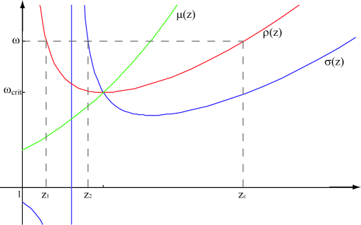
Figure 1. The curves $\rho(z)$ (3.9), $\sigma(z)$ (3.12), and $\mu(z)$ intersect each other at the local minimum of $\rho(z)$, attained for $z=\tfrac{1+\sqrt{3}}{2},\,\rho(z)=\omega_{\mathrm{crit}}$ (see Theorem 2.1).

For the acceptable range of $\omega$, that is $\omega>\omega_{\mathrm{crit}}$ (see Theorem 2.1), there exists a unique value $z_{1}$ that satisfies (3.10a) and such that $k(z_{0})>0$. From (3.10b), we have that also $\frac{\partial w}{\partial z}(z_{1},0)>0$. This means that the Jacobian (3.8) has two positive eigenvalues and therefore we have part (1) of the claim, with an infinite number of radial geodesics tending to this equilibrium point, for every $\ell\geq 0$. Note that this situation (1) cover also radial geodesic existence, that is when $\ell=0$. Using (3.6), the curves $R(r)$ behaves like $R(r)=\alpha z_{1}^{2}r^{3}+o(r^{3})$.

If $\omega>\omega_{\mathrm{crit}}$, from Figure 1 we see that there exists another values of $z=z_{c}$ satisfying $\rho(z_{c})=\omega$. In this case we have two negative eigenvalues of (3.8). With reference to the system put in the form (3.5), the equilibrium is again hyperbolic, but the stable manifold has dimension 1, and therefore a single null geodesic tending to the equilibrium exists. Actually, it can be shown that this geodesic is radial, since it can be seen that at least a radial null geodesic tending to the equilibrium exists. Indeed, radial geodesics are solutions of the ODE (3.7a) under the assumption $\ell=0$. We can easily see that $z=z_{c}$ is an equilibrium of (3.7a), such that there exist a unique solution tending to this equilibrium. Since radial geodesics are solutions of (3.7a)–(3.7b) with $\ell q\equiv 0$, we conclude that the (unique) solution of (3.7a)–(3.7b) must be radial. The corresponding $x=\alpha z_{c}^{2}$ represents Cauchy horizon direction.

We also note that the corresponding function $R_{c}(r)$ must bound from above any other geodesic $R_{g}(r)$. Of course, this must be true for any other radial geodesic near $r=0$, and therefore for any other value of $r$ by uniqueness of Cauchy problem solution. Let us show that this also holds true for nonradial geodesic. By contradiction, let $R_{g}(r)$ be a nonradial geodesic, such that its projection on the $(r,R)$ plane bounds from above $R_{c}(r)$ for some $r_{*}$, that is $R_{g}(r_{*})>R_{c}(r_{*})$. Since $R_{g}(r)$ is a subsolution of radial null geodesic equation, and $R_{c}(r)$ is a solution of the same ODE, therefore we can find a radial null geodesic $R_{n}(r)$ with initial data $R_{n}(r_{*})\in]R_{c}(r_{*}),R_{g}(r_{*})[$, and trace it back until $R_{n}(0)=0$, obtaining a radial geodesic $R_{n}(r)>R_{c}(r)$ in a right neighborhood of $r=0$, which as said before is absurd, and claim (3) is complete.

Let us now discuss case (b) to get claim (2) of the Proposition.

We first observe that this time it must be $k(z)>0$ otherwise we have no equilibria. Arguing as in the previous case, we find that the determinant of the Jacobian in the equilibrium – say $(z_{2},\sqrt{\frac{k(z_{2})}{h(z_{2})}})$ – is given by

(3.11) $$-2k(z_{2})\frac{\mathrm{d}w(z,\sqrt{\frac{k(z)}{h(z)}})}{\mathrm{d}z}|_{z=z_{2}}.$$

The root function in this case is given by

(3.12) $$\sigma(z)=\frac{4z^{5}}{2z^{2}-3},$$

which has the properties

(3.13a) $$w(z_{2},\sqrt{\frac{k(z_{2})}{h(z_{2})}})=0\,\Leftrightarrow\,\sigma(z_{2})=\omega,$$

(3.13b) $$\frac{\partial w}{\partial z}(z_{2},\sqrt{\frac{k(z_{2})}{h(z_{2})}})=-\gamma^{2}\sigma^{\prime}(z_{2}),$$

where $\gamma$ is some non vanishing constant. The situation is depicted in Figure 1. For any $\omega>\omega_{\mathrm{crit}}$ there exists a unique value of $z_{2}$ satisfying (3.13a) with $k(z_{2})>0$. Using (3.13b), we get that the quantity (3.11) is negative and then there exists one and only one positive eigenvalue of the Jacobian, which results in the existence of infinite non radial null geodesic such that the corresponding $R(r)$ behaves like $R(r)=\alpha z_{2}^{2}r^{3}+o(r^{3})$. Indeed, the stable manifold of the system put in the form (3.5) has dimension 2.

Notice that, in this case, there are no other choice available since the other root of the equation $\sigma(z)=\omega$ lies in the $\{k<0\}$ region.

To complete the proof, let us now analyze the behavior of the angular function $\phi(r)$. Using (3.3b), and the above estimates,

(3.14) $$\frac{\mathrm{d}\phi}{\mathrm{d}r}\cong\ell\left(\frac{h(z)}{z}\right)\frac{q}{r}.$$

For a non radial geodesic from case (1), $q\to 0$ as $r\to 0^{+}$, and then, from (3.7b), $\frac{\mathrm{d}q}{\mathrm{d}r}\cong k(z_{1})\tfrac{q}{r}$, from which $q(r)\cong r^{k(z_{1})}$, and then, using (3.14), $\phi(r)$ has a finite limit as $r\to 0^{+}$.

For a non radial geodesic from case (2) conversely, $q$ tends to a finite positive value and then the function $\phi(r)$ goes like $k\,r^{-1}$, which determines a negative diverging behavior of the function $\phi(r)$. ∎

Remark 3.3.

These results are completely consistent with the analysis carried out in [12, 14], which have established a double topological nature of the naked singularity in the particular case of dust solution under self–similarity assumption. In particular, case (1) corresponds to a region of the singularity foliated by a 2–sphere, whereas case (2) corresponds to a topologically pointwise singular region.

Remark 3.4.

If we look at the behavior of the quantity $k^{2}R_{\alpha\beta}K^{\alpha}K^{\beta}$ along null radial geodesics, where $R_{\alpha\beta}$ is Ricci tensor, $K^{\alpha}=\tfrac{\mathrm{d}x^{\alpha}}{\mathrm{d}k}$ is the tangent vector of the geodesic with parameter $k$, we get

(3.15) $$k^{2}\,R_{\alpha\beta}K^{\alpha}K^{\beta}=\frac{k^{2}\Psi_{,r}}{4\pi R^{2}u^{3}G\,Y}(K^{R})^{2}.$$

In view of the above theorem, equations (3.2) and (3.3a) ensure that there exists $\lim_{k\to 0^{+}}K^{R}$, then $\tfrac{k}{R}K^{R}$ tends to a finite nonzero limit value. Since both $G$ and $\Psi_{,r}$ goes like $r^{2}$, and $Y,u$ tends to a finite nonzero limit along the geodesics, the quantity in (3.15) goes to a finite nonzero value. It follows that these null geodesics terminate in a strong curvature singularity in the sense of Tipler [17].

4. Faraway visibility of the singularity

4.1. Size of the singularity

In the following, we will study the behavior at infinity of null geodesics emanating from the singularity. We have already seen that there exists an infinite number of light rays escaping from the trapped region; These geodesics arrives at the boundary of the collapsing sphere of anisotropic matter with some value $R(r_{b})$, and they have to be continued by studying the behavior of null geodesics in the external region (2.7) escaping from the boundary and such that $R=R(r_{b})$.

The equation for null geodesics – that, without loss of generality, we will suppose to lie in the subspace $\{\theta=\tfrac{\pi}{2}\}$ – is given by

(4.1) $$\frac{\mathrm{d}T}{\mathrm{d}\kappa}=\frac{\omega}{\chi(R)},\quad\frac{\mathrm{d}R}{\mathrm{d}\kappa}=\omega\sqrt{1-\frac{\chi(R)}{R^{2}}\left(\frac{\ell}{\omega}\right)^{2}},\quad\frac{\mathrm{d}\theta}{\mathrm{d}\kappa}=0,\quad\frac{\mathrm{d}\phi}{\mathrm{d}\kappa}=\frac{\ell}{R^{2}},$$

where $\kappa$ denotes as usual the affine parameter and $\ell$ and $\omega$ are constant of motion.

As explained in [12], since the metric (2.7) does not depend on $T$ we can uniquely associate to an observer $R=R_{0}$ an orthonormal basis of the tangent space to a point $(T,R_{0},\theta,\phi)$ of the outer region (i.e. such that $R_{0}>2M(R_{0})$), which will be denoted by

$$\left\{e_{(T)}=\chi(R_{0})^{-1/2}\partial_{T},\,e_{(R)}=\chi(R_{0})^{1/2}\partial_{R},\,e_{(\theta)}=R_{0}^{-1}\partial_{\theta},\,e_{(\phi)}=(R_{0}\sin\theta)^{-1}\partial_{\phi}\right\}.$$

Then, if we consider a null geodesic with affine parameter $\kappa$ emanating from the singularity passing for $R=R_{0}$, and denote by $\kappa^{\alpha}=\frac{\mathrm{d}X^{\alpha}}{\mathrm{d}\kappa}$ its tangent vector, this observer measures an angle $\delta$ between the light ray and the radial direction equal to

(4.2) $$\delta=\arctan\left(\frac{g_{\mu\alpha}e_{(\phi)}^{\mu}\kappa^{\alpha}}{g_{\mu\alpha}e_{(R)}^{\mu}\kappa^{\alpha}}\right)=\frac{\ell}{\omega}\sqrt{\frac{\chi(R_{0})}{R_{0}^{2}-(\ell/\omega)^{2}\chi(R_{0})}}.$$

The above quantity depends on the geodesic, and therefore the supremum made among the set ${\mathfrak{S}}$ of all singular geodesics detected at $R=R_{0}$ gives a measure of the singularity detected by the observer. One can conceive the righthand side above, fixing $R_{0}$, as a function in $(\ell/\omega)$ which results to be increasing. Therefore, the “size” of the singularity detected by the faraway observer is related to the quantity

$$b:=\sup_{\mathfrak{S}}\frac{\ell}{\omega},$$

which can be regarded [12] as a sort of impact parameter.

Using this definition, it is not hard to prove an extension of the result already proved for the particular case studied in [12].

Proposition 4.1.

If the boundary of the interior region $r=r_{b}$ is sufficiently small, then the non radial geodesics of largest impact parameters emanating from the singularity are such that the angular function $\phi\to-\infty$ in the approach to the singularity (case (2) of Proposition 3.2, see also Remark 3.3).

Proof.

Of course, we will consider only nonradial geodesics, when $\ell\not=0$.

Using continuity of the metric along the junction hypersurface, one gets

(4.3) $$\frac{\mathrm{d}T}{\mathrm{d}\kappa}=\frac{\mathrm{d}T}{\mathrm{d}R}\frac{\mathrm{d}R}{\mathrm{d}\kappa}+\frac{\mathrm{d}T}{\mathrm{d}r}\frac{\mathrm{d}r}{\mathrm{d}\kappa}=\left[-\frac{Y}{\chi\,u}\frac{\mathrm{d}R}{\mathrm{d}r}+G\right]\frac{\mathrm{d}r}{\mathrm{d}\kappa},$$

and using (4.1), together with (3.2)–(3.3b) one finds the angular frequency $\omega$ and therefore the impact parameter $b$, which is given by

(4.4) $$b=\sup_{\mathfrak{S}}\left(\frac{R(r)\,\ell q(r)}{Y(r,R(r))\sqrt{u^{2}(r,R(r))+(\ell q(r))^{2}}-u^{2}(r,R(r))}\right)|_{r=r_{b}}.$$

With reference to the cases listed in Proposition 3.2, let $R_{1}(r)$ be a nonradial geodesic from case (1), and let $R_{2}(r)$ a (necessarily non radial) geodesic from case (2). It is easy to verify that, as $r\to 0^{+}$, the quantity in round brackets in (4.4) tends to 0 along $R_{1}(r)$ and tends to a finite nonzero value along $R_{2}(r)$. Then, if $r_{b}$ is sufficiently small, we can suppose that this quantity, along $R_{2}$, bounds from above the same quantity computed along $R_{1}$ until $r=r_{b}$. ∎

4.2. Redshift

Following [4], the frequency shift $z$ between a source and an observer respectively located at events $P_{1}$ and $P_{2}$, connected by a null geodesic with tangent vector $\overrightarrow{\kappa}$ w.r.t. the affine parameter, is defined as

(4.5) $$1+z=\frac{g_{P_{1}}(\overrightarrow{\kappa},u_{(s)})}{g_{P_{2}}(\overrightarrow{\kappa},u_{(o)})}.$$

where $u_{(s)}$ and $u_{(o)}$ are the 4–velocities of the source and the observer respectively.

To determine the redshift associated to the singular geodesics, the numerator above will be replaced by a limit expression as $P_{1}$ approaches the central singularity. Let us therefore consider a singular geodesic passing at event $P_{2}$ in the exterior space such that $R(P_{2})=R_{0}$. Using the basis (4.3), together with (4.1), it is easy to see that the denominator in (4.5) is given by $-\chi(R_{0})^{1/2}\omega$, which under the hypothesis (2.8) is always finite also if $R_{0}$ tends to infinity. On the other side, the velocity field in the interior spacetime is given by $-u(r,R)\partial_{R}$, and using (3.2)–(3.3a) one finds that the absolute value of the numerator in (4.5) is given by

(4.6) $$\lim_{r\to 0^{+}}\frac{1}{R(r)}\left[\left(\frac{u(r,R(r))}{q(r)}\right)^{2}+\ell^{2}\right]^{1/2}=+\infty,$$

which results in an infinite frequency shift. Actually we can observe that calculation of (4.6) above seems a feature of all singular spherically symmetric models, at least for nonradial geodesics, when $\ell\not=0$. In the case under our study, moreover, (4.6) holds also for radial geodesic since, using Proposition 3.2 and equation (2.2c), $u(r,R(r))\cong u_{0}\neq 0$, and both $R(r)$ and $q(r)$ are infinitesimal. It appears also to be possible the study of the limit in (4.6) in a even more general framework, and work in this direction is in progress.

All in all, these models shows the same feature described in [4] for dust solutions: in the case corresponding to a strong naked singularity (along radial geodesic), null geodesics are infinitely redshifted. Therefore, it can be said that there exists a form of weak censorship for such class of solutions, at least at the classical level. Of course however, quantum phenomena might change this scenario, as suggested by some authors (see [12],[13]).

5. Discussion and conclusions

In this paper we have studied visibility of the naked singularity for a faraway observer, investigating global behavior of null (radial and nonradial) geodesics in a class of spherically symmetric singular spacetimes. The interior part belongs to a wide class of anisotropic solutions; as known from the analysis carried out in [7], the endstate of the central singularity is determined by the lower order term $n$ of Taylor development of a quantity determined by the metric. In this paper we considered the case $n=3$, which has a special interest since (i) the endstate is determined by the value of a certain parameter $\xi/\alpha$, that causes a sort of ”phase transition” between naked singularity and black hole situations, and (ii) radial geodesics terminates into a strong curvature singularity, as observed in Remark 3.4.

The exterior part belongs to the class of anisotropic generalization of de Sitter solution discussed in [5]. The form of the metric closely resembles the Schwarzschild line element, but the mass here depends on the areal coordinate $R$ since a constant mass would not properly match an interior solution with non vanishing radial pressures. Indeed, if Misner–Sharp masses for both solutions (interior and exterior) coincide at a hypersurface $r=\text{const.}$, this ensures Darmois junction conditions to hold along this hypersurface.

Existence of nonradial geodesics is crucial to investigate global visibility. The system of ODE satisfied by the nonradial geodesics does not decouple and the most suitable way seems to study equilibrium points of this system. It turns out that there are two values $x_{1}<x_{2}$, depending on the data of the spacetime, such that there is an infinite number of nonradial geodesic $R(r)$ emanating with ”direction” $x_{1}$ (i.e. such that $\lim_{r\to 0}R(r)/r^{3}=x_{1}$) and infinite nonradial geodesics with direction $x_{2}$. This result is not in contrast with previous results regarding self similar collapse [14] where one has infinite geodesic with direction $x_{1}$ vs. only one geodesic with direction $x_{2}$. Indeed, as the proof of Proposition 3.2 points out, the stable manifold of the equilibrium has dimension 3 in the first case and 2 in the second one. Self–similarity assumption simplifies the geometry of these stable manifolds, shrinking them by one dimension.

It must be remarked that a crucial fact is that ODE system can be brought in the form (3.4), where the equilibria are all hyperbolic. This is a feature of all collapsing matter models known in literature, which excluded pathological situations such as the ones outlined in [13], and explains why the so-called root equation method repeatedly exploited in previous works – based on the existence of a certain limit which in principle cannot be taken for granted (see for instance [2, 3, 12]) – leads all the same to the conclusions one would expect.

The analysis of the ODE system allowed us to determine a sort of ”impact parameter” that characterizes the ”size” of the singularity as it is seen by a faraway observer. It turns out that photons emanated by the naked singularity are infinitely redshifted also when pressures are present, as has been already shown (see [4]) for the – pressureless – Tolman–Bondi collapse.

References

- [1] C. J. S. Clarke and A. Krolak, J. Geom. Phys. 2 (1985) 127
- [2] S. S. Deshingkar, P. S. Joshi, and I. H. Dwiwedi, Phys.Rev. D65 (2002) 084009
- [3] I. H. Dwiwedi, P. S. Joshi, Commun. Math. Phys. 166 (1994) 117
- [4] I. H. Dwivedi, Phys. Rev. D 58, 064004 (1998)
- [5] R. Giambò, Class. Quantum Grav 19 (2002) 4399
- [6] R. Giambò, Class. Quantum Grav. 22 (2005) 2295
- [7] R. Giambò, F. Giannoni, G. Magli, P. Piccione, Commun. Math. Phys. 235(3), 545-563 (2003).
- [8] F. Giannoni, On Gravitational Collapse in Spherical Symmetry, Proceedings of Workshop ”Dymamics and Thermodynamics of Blackholes and Naked Singularities”, online version on http://www.mate.polimi.it/bh, Politecnico di Milano (2004)
- [9] W. Israel, Nuovo Cim. 44B (1966) 1, Nuovo Cim. 49B (1966) 463 (erratum)
- [10] P. S. Joshi, Gravitational Collapse End States, Proceedings of Workshop ”Dymamics and Thermodynamics of Blackholes and Naked Singularities”, online version on http://www.mate.polimi.it/bh, Politecnico di Milano (2004)
- [11] G. Magli, Class. Quantum Grav. 14 1937 (1997)
- [12] K. Nakao, N. Kobayashi, and H. Ishihara, Phys. Rev. D 67, 084002 (2003)
- [13] B. C. Nolan and F. C. Mena, Class. Quantum Grav. 18 4531 (2001)
- [14] B. C. Nolan and F. C. Mena, Class. Quantum Grav. 19, 2587 (2002)
- [15] A. Ori, Class. Quantum. Grav. 7 985 (1990)
- [16] J. Palis, jr., W. de Melo, Geometric Theory of Dynamical Systems – An Introduction, Springer–Verlag, 1982
- [17] F. J. Tipler, Phys. Lett. 64A (1987) 8
- [18] F. J. Tipler, C. J. S. Clarke, and G. F. R. Ellis, in General Relativity and Gravitation Vol. 2 (ed. A Held), Plenum NY (1980)