Gravitational wave bursts from cosmic (super)strings: Quantitative analysis and constraints

Abstract

We discuss data analysis techniques that can be used in the search for gravitational wave bursts from cosmic strings. When data from multiple interferometers are available, we describe consistency checks that can be used to greatly reduce the false alarm rates. We construct an expression for the rate of bursts for arbitrary cosmic string loop distributions and apply it to simple known solutions. The cosmology is solved exactly and includes the effects of a late-time acceleration. We find substantially lower burst rates than previous estimates suggest and explain the disagreement. Initial LIGO is unlikely to detect field theoretic cosmic strings with the usual loop sizes, though it may detect cosmic superstrings as well as cosmic strings and superstrings with non-standard loop sizes (which may be more realistic). In the absence of a detection, we show how to set upper limits based on the loudest event. Using Initial LIGO sensitivity curves, we show that these upper limits may result in interesting constraints on the parameter space of theories that lead to the production of cosmic strings.

I Introduction

Cosmic strings can form during phase transitions in the early universe kibble76 . Although cosmic microwave background data has ruled out cosmic strings as the primary source of density perturbations, they are still potential candidates for the generation of a host of interesting astrophysical phenomena including gravitational waves, ultra high energy cosmic rays, and gamma ray bursts. For a review see alexbook .

Following formation, a string network in an expanding universe evolves toward an attractor solution called the “scaling regime” (see alexbook and references therein). In this regime, the statistical properties of the system, such as the correlation lengths of long strings, scale with the cosmic time, and the energy density of the string network becomes a small constant fraction of the radiation or matter density.

The attractor solution arises due to reconnections, which for field theoretic strings essentially always occur when two string segments meet. Reconnections lead to the production of cosmic string loops, which in turn shrink and decay by radiating gravitationally. This takes energy out of the string network, converting it to gravitational waves. If the density of strings in the network becomes large, then strings will meet more often, thereby producing extra loops. The loops then decay gravitationally, removing the surplus energy from the network. If, on the other hand, the density of strings becomes too low, strings will not meet often enough to produce loops, and their density will start to grow. Thus, the network is driven toward a stable equilibrium.

Recently, it was realised that cosmic strings could be produced in string-theory inspired inflation scenarios tye1 ; tye2 ; alex15 ; tye3 ; cmp . These strings have been dubbed cosmic superstrings. The main differences between field theoretic strings and superstrings are that the latter reconnect when they meet with probabilities $p$ that can be less than $1$, and that more than one kind of string can form. The values suggested for $p$ are in the range $10^{-3}-1$ jjp . The suppressed reconnection probabilities arise from two separate effects. The first is that fundamental strings interact probabilistically, and the second that strings moving in more than $3$ dimensions may more readily avoid reconnections: Even though two strings appear to meet in $3$ dimensions, they miss each other in the extra dimensions alex15 .

The effect of a small reconnection probability is to increase the time it takes the network to reach equilibrium, and to increase the density of strings $\rho$ at equilibrium. The amount by which the density is increased is the subject of debate, with predictions ranging from $\rho\propto p^{-2}$, to $\rho\propto p^{-0.6}$ tye3 ; mairi ; shellardlowp . In this work we will assume the density scales like $\rho\propto p^{-1}$, and that only one kind of cosmic superstring is present DV2 .

Cosmic strings and superstrings can produce powerful bursts of gravitational waves. These bursts may be detectable by first generation interferometric earth-based gravitational wave detectors such as LIGO and VIRGO DV2 ; DV0 ; DV1 . Thus, the exciting possibility arises that a certain class of string theories may have observable consequences in the near future pol1 . It should be noted that if the hierarchy problem is solved by supersymmetry then the detectability of bursts produced by cosmic superstrings is strongly constrained due to dilaton emission babichev .

The bursts we are most likely to be able to detect are produced at cosmic string cusps. Cusps are regions of string that acquire phenomenal Lorentz boosts, with gamma factors $\gamma\gg 1$. The combination of the large mass per unit length of cosmic strings and the Lorentz boost results in a powerful burst of gravitational waves. The formation of cusps on cosmic string loops and long strings is generic, and their gravitational waveforms are simple and robust kenandi .

The three LIGO interferometers (IFOs) are operating at design sensitivity. The VIRGO IFO is in the final stages of commissioning. Thus, there arises a need for a quantitative and observationally driven approach to the problem of bursts from cosmic strings. This paper attempts to provide such a framework.

We consider the data analysis infrastructure that can be used in the search for gravitational wave bursts from cosmic string cusps, as well as cosmological burst rate predictions.

The optimal method to use in the search for signals of known form is matched-filtering. In Sec. II we discuss the statistical properties of the matched-filter output, template bank construction, an efficient algorithm to compute the matched-filter, and, when data from multiple interferometers is available, consistency checks that can be used to greatly reduce the false alarm rate. In Sec. III we discuss the application of the loudest event method to set upper limits on the rate, the related issue of sensitivity, and background estimation. In Sec. IV we derive an expression for the rate of bursts for arbitrary cosmic string loop distributions, and apply it to the distribution proposed in Refs. DV2 ; DV0 ; DV1 . In Sec. V we compare our estimates for the rate with results suggested by previous estimates (in DV2 ; DV0 ; DV1 ). We find substantially substantially lower event rates. The discrepancy arises primarily from our estimate of a detectable burst amplitude, and the use of a cosmology that includes the late-time acceleration. We also compute the rate for simple loop distributions, using the results of Sec. IV and show how the detectability of bursts is sensitive to the loop distribution. In Sec. VI we discuss how, in the absence of a detection, it is possible to use the upper limits on the rate discussed in Sec. III to place interesting constraints on the parameter space of theories that lead to the production of cosmic strings. We show an example of these constraints. We summarise our results and conclude in Sec. VII.

II Data analysis

II.1 The signal

In the frequency domain, the waveforms for bursts of gravitational radiation from cosmic string cusps are given by DV0 ,

$$h(f)=A|f|^{-4/3}\Theta(f_{h}-f)\,\Theta(f-f_{l}).$$ (1)

The low frequency cutoff of the gravitational wave signal, $f_{l}$, is determined by the size of the feature that produces the cusp. Typically this scale is cosmological. In practice, however, the low frequency cutoff of detectable radiation is determined by the low frequency behaviour of the instrument (for the LIGO instruments, for instance, by seismic noise). The high frequency cutoff, on the other hand, depends on the angle $\theta$ between the line of sight and the direction of the cusp. It is given by,

$$f_{h}\sim\frac{2}{\theta^{3}L},$$ (2)

where $L$ is the size of the feature that produces the cusp, and in principle can be arbitrarily large. The amplitude parameter of the cusp waveform $A$ is,

$$A\sim\frac{G\mu L^{2/3}}{r},$$ (3)

where $G$ is Newton’s constant, $\mu$ is the mass per unit length of strings, and $r$ is the distance between the cusp and the point of observation. We have taken the speed of light $c=1$.

The time domain waveform can be computed by taking the inverse Fourier transform of Eq. (1). The integral has a solution in terms of incomplete Gamma functions. For a cusp with peak arrival time at $t=0$ it can be written as

$$h(t)=2\pi A|t|^{1/3} \{ i\Gamma(-1/3,2\pi if_{l}t)+c.c.$$ (4)

$$- [i\Gamma(-1/3,2\pi if_{h}t)+c.c.]\}.$$

The duration of the burst is on the order of the inverse of the the low frequency cutoff $f_{l}$, and the spike at $t=0$ is rounded on a timescale $\sim 1/f_{h}$.

Eq. (4) is useful to make a rough estimate the amplitude of changes in the strain $h(t)$ that a cusp would produce. If we consider a time near $t=0$, we can expand the incomplete Gamma functions according to gradryz ,

$$\Gamma(\alpha,x)=\Gamma(\alpha)+\sum_{n=0}^{\infty}\frac{(-1)^{n}x^{\alpha+n}}{n!(\alpha+n)}.$$ (5)

Keeping the first term of the sum we see that the amplitude in strain of the cusp is,

$$\Delta h_{\text{cusp}} = 6A(f_{l}^{-1/3}-f_{h}^{-1/3})$$ (6)

$$\approx 6Af_{l}^{-1/3},\,\,\,f_{h}\gg f_{l}.$$

II.2 Definitions and conventions

The optimal method to use in the search for signals of known form is matched-filtering. For our templates we take

$$t(f)=f^{-4/3}\Theta(f_{h}-f)\,\Theta(f-f_{l}),$$ (7)

so that a signal would have $h(f)=A\,t(f)$. We define the usual detector-noise-weighted inner product cutlerflanagan ,

$$(x|y)\equiv 4\Re\int_{0}^{\infty}df\,\frac{x(f)y^{*}(f)}{S_{h}(f)},$$ (8)

where $S_{h}(f)$ is the single-sided spectral density defined by $\langle n(f)n^{*}(f^{\prime})\rangle=\frac{1}{2}\delta(f-f^{\prime})S_{h}(f)$, where $n(f)$ is the Fourier transform of the detector noise.

The templates of Eq. (7) can be normalised by the inner product of a template with itself,

$$\sigma^{2}=(t|t)$$ (9)

so that,

$${\hat{t}}=t/\sigma,\quad\mbox{and}\quad({\hat{t}}|{\hat{t}})=1.$$ (10)

If the output of the instrument is $s(t)$, the signal to noise ratio (SNR) is defined as,

$$\rho\equiv(s|{\hat{t}}).$$ (11)

In general, the instrument output is a burst $h(t)$ plus some noise $n(t)$, $s(t)=h(t)+n(t)$. When the signal is absent, $h(t)=0$, the SNR is Gaussian distributed with zero mean and unit variance,

$$\langle\rho\rangle=\langle(n|{\hat{t}})\rangle=0,\,\,\,\,\langle\rho^{2}\rangle=\langle(n|{\hat{t}})^{2}\rangle=1.$$ (12)

When a signal is present, the average SNR is

$$\langle\rho\rangle = \langle(h|{\hat{t}})\rangle+\langle(n|{\hat{t}})\rangle=(A\sigma{\hat{t}}|{\hat{t}})=A\sigma,$$ (13)

and the fluctuations have variance

$$\langle\rho^{2}\rangle-\langle\rho\rangle^{2}=\langle(h+n|{\hat{t}})^{2}\rangle-A^{2}\sigma^{2}=1.$$ (14)

Thus, when a signal of amplitude $A$ is present, the signal to noise ratio measured, $\tilde{\rho}$ , is a Gaussian random variable, with mean $A\sigma$ and unit variance,

$$\tilde{\rho}=A\sigma\pm 1$$ (15)

The amplitude that we assign the event $\tilde{A}$ depends on the template normalisation $\sigma$,

$$\tilde{A}=\frac{\tilde{\rho}}{\sigma}=A\pm\frac{1}{\sigma}.$$ (16)

This means that in the presence of Gaussian noise the relative difference between measured and actual signal amplitudes will be proportional to the inverse of the SNR,

$$\frac{\Delta A}{A}=\pm\frac{1}{\langle\rho\rangle}.$$ (17)

If an SNR threshold $\rho_{\text{th}}$ is chosen for the search, on average only events with amplitude

$$A_{\text{th}}\geq\frac{\rho_{\text{th}}}{\sigma},$$ (18)

will be detected.

II.3 Template bank

Cosmic string cusp waveforms have two free parameters, the amplitude and the high frequency cutoff. Since the amplitude is an overall scale, the template need not match the signal amplitude. However, the high frequency cutoff does affect the signal morphology, so a bank of templates is needed to match possible signals.

The template bank, $\{t_{i}\}$, where $i=1,2,\dots N$, is one-dimensional, and fully specified by a collection of high frequency cutoffs $\{f_{i}\}$. The number of templates $N$ should be large enough to cover the parameter space finely. We choose the ordering of the templates so that $f_{i}>f_{i+1}$.

Although in principle the high frequency cutoff can be infinite, in practice the largest distinguishable high frequency cutoff is the Nyquist frequency of the time-series containing the data, $f_{\text{Nyq}}=1/(2\Delta t)$, where $\Delta t$ is the sampling time of that time-series. The normalisation factor for the first template is given by

$$\sigma^{2}_{1}=(t_{1}|t_{1})=4\Re\int_{f_{l}}^{f_{\text{Nyq}}}df\,\frac{f^{-8/3}}{S_{h}(f)}.$$ (19)

This template is the one with the largest $\sigma$, and thus the largest possible SNR at fixed amplitude.

To determine the high frequency cutoffs of the remaining templates, we proceed as follows. The fitting factor between two adjacent templates $t_{i}$ and $t_{i+1}$, with high frequency cutoffs $f_{i}$ and $f_{i+1}$, is defined as fittingfactor

$$F=\frac{(t_{i}|t_{i+1})}{\sqrt{(t_{i}|t_{i})(t_{i+1}|t_{i+1})}}=1-\epsilon,$$ (20)

where $\epsilon$ is the maximum mismatch we choose to allow. The maximum mismatch is twice the maximum fractional SNR loss due to mismatch between a template in the bank and a signal, and should be small. Since $t_{i+1}$ has a lower frequency cutoff than $t_{i}$,

$$(t_{i}|t_{i+1})=(t_{i+1}|t_{i+1}).$$ (21)

Thus, the maximum mismatch is,

$$\epsilon=1-\sqrt{\frac{(t_{i+1}|t_{i+1})}{(t_{i}|t_{i})}}=1-\frac{\sigma_{i+1}}{\sigma_{i}},$$ (22)

and once fixed, determines the high frequency cutoff $f_{i+1}$, given $f_{i}$. Thus the template bank can be constructed iteratively.

II.4 Single interferometer data analysis

A convenient way to apply the matched-filter is to use the inverse spectrum truncation procedure invspectrunc . The usual implementation of the procedure involves the creation of an FIR (Finite Impulse Response) digital filter for the inverse of the single-sided power spectral density, $S_{h}(f)$, of some segment of data. This filter, along with the template can then be efficiently applied to the data via FFT (Fast Fourier Transform) convolution. Here we describe a variation of this method in which the template as well as $S_{h}(f)$ are incorporated into the digital filter.

Digital filters may be constructed for each template $j$ in the bank as follows. First we define a quantity which corresponds to the square root of our normalised template divided by the single-sided power spectral density,

$$T_{j,1/2}(f)=\sqrt{\frac{{\hat{t}}_{j}(f)}{S_{h}(f)}}.$$ (23)

This quantity is then inverse Fourier transformed to create,

$$T_{j,1/2}(t)=\int dfe^{2\pi ift}T_{j,1/2}(f).$$ (24)

At this point the duration of the filter is identical to the length of data used to estimate the power spectrum $S_{h}(f)$. We then truncate the filter, setting to zero values of the filter sufficiently far from the peak. This is done to limit the amount of data corrupted by filter initialisation. After truncation, however, the filter still needs to be sufficiently long to adequately suppress line noise in the data (such as power line harmonics). The truncated filter is then forward Fourier transformed, and squared, creating the frequency domain FIR filter $T_{j}(f)$. The SNR is the time-series given by,

$$\rho_{j}(t)=4\Re\int_{0}^{\infty}df\,s(f)T_{j}(f)e^{2\pi ift}.$$ (25)

where $s(f)$ is a Fourier transform of the detector strain data.

To generate a discrete set of events or triggers we can take the SNR time series for each template $\rho_{j}(t)$ and search for clusters of values above some threshold $\rho_{\text{th}}$. We identify these clusters as triggers and determine the following properties: 1) The SNR of the trigger which is the maximum SNR of the cluster; 2) the amplitude of the trigger, which is the SNR of the trigger divided by the template normalisation $\sigma_{j}$; 3) the peak time of the trigger, which is the location in time of the maximum SNR; 4) the start time of the trigger, which is the time of the first SNR value above threshold; 5) the duration of the trigger, which includes all values above the threshold; and 6) the high frequency cutoff of the template. The final list of triggers for some segment of data can then be created by choosing the trigger with the largest SNR when several templates contain triggers at the same time (within the durations of the triggers).

The rate of events we expect can be estimated for the case of white Gaussian noise. In the absence of a signal the SNR is Gaussian distributed with unit variance. Therefore, at an SNR threshold of $\rho_{\text{th}}$, the rate of events with $\rho>\rho_{\text{th}}$ we expect with a single template is

$$R(>\rho_{\text{th}})\approx\Delta t^{-1}{\text{Erfc}}(\rho_{\text{th}}/\sqrt{2})$$ (26)

where $\Delta t$ is the sampling time of the SNR time series, and Erfc is the complementary error function. For example, if the time series is sampled at $4096$ Hz and an SNR threshold of $4$ is used we expect a false alarm rate of $R(>4)\approx 0.26$ Hz. The rate of false alarms rises exponentially with lower thresholds.

II.5 Multiple interferometer consistency checks

When data from multiple interferometers is available, a coincidence scheme can be used to greatly reduce the false alarm rate of events. For example, in the case of the three LIGO interferometers, using coincidence would result in a coincident false alarm rate of

$$R=R_{\text{H1}}R_{\text{H2}}R_{\text{L1}}(2\Delta\tau_{\text{HH}})(2\Delta\tau_{\text{HL}}),$$ (27)

where $R_{\text{H1}}$ and $R_{\text{H2}}$ are the rate of false triggers in the $4$ km and $2$ km IFOs in Hanford, WA, and $R_{\text{L1}}$ is the rate of false triggers in the $4$ km IFO in Livingston, LA. The two time windows $\Delta\tau_{\text{HH}}$, and $\Delta\tau_{\text{HL}}$ are the maximum allowed time differences between peak times for coincident events in the H1 and H2 IFOs, and H1-L1 (or H2-L1), respectively. Eq. (27) follows trivially if the events are Poisson distributed. The factors of $2$ multiplying the time windows arise from the fact that an event in the trigger set of one instrument will survive the coincidence if there is an event in the other instrument within a time $\Delta\tau$ on either side. The time windows should allow for light-travel time between sites, shifting of measured peak location due to noise, timing errors and calibration errors. For example, if we take $\Delta\tau_{\text{HL}}=12$ ms and $\Delta\tau_{\text{HH}}=2$ ms, which allows for the light travel time of $10$ ms between the Hanford and Livingston sites as well as $2$ ms for other uncertainties, and the single IFO false alarm rate estimated in the previous subsection ($0.26$ Hz), we obtain a triple coincident false alarm rate,

$$R\approx 1.7\times 10^{-6}\,\text{Hz},$$ (28)

which is about $50$ false events per year.

Additionally, when two instruments are co-aligned, such as the H1 and H2 LIGO IFOs, we can demand some degree of consistency in the amplitudes recovered from the matched-filter (see, for example, the distance cut used in amplitudecut ). If the instruments are not co-aligned then the amplitudes recovered by the matched-filter could be different. This is due to the fact that the antenna pattern of the instrument depends on the source location in the sky. If the event is due to a fluctuation of the noise or an instrumental glitch we do not generally expect the amplitudes in two co-aligned IFOs to agree. The effect of Gaussian noise to $1$ $\sigma$ on the estimate of the amplitude can be read from Eq. (17). This equation can be used to construct an amplitude veto. For example, to veto events in H1 we can demand

$$\frac{A_{\text{H1}}-A_{\text{H2}}}{A_{\text{H1}}}<\pm\left(\frac{\delta}{\rho_{\text{H1}}}+\kappa\right),$$ (29)

where $\delta$ is the number of standard deviations we allow and $\kappa$ is an additional fractional difference in the amplitude that accounts for other sources of uncertainty (such as the calibration).

These tests can be used to construct the final trigger set, a list of survivors for each of our instruments which have passed all the consistency checks.

III Upper limits, sensitivity and background

In this section we describe the application of the loudest event method loudestevent to our problem, address the related issue of sensitivity, and discuss background estimation.

We define the loudest event to be the survivor with the largest amplitude. Suppose, in one of the instruments, we find the loudest event to have an amplitude $A^{*}$. For an observation time $T$, on average, the number of events we expect to show up with an amplitude greater than $A^{*}$ is

$$N_{>A^{*}}=T\gamma,$$ (30)

where the effective rate is defined as

$$\gamma=\int_{0}^{\infty}\epsilon(A^{*},A)\frac{dR(A)}{dA}dA.$$ (31)

Here, $\epsilon(A^{*},A)$ is the search efficiency, namely the fraction of events with an optimally oriented amplitude $A$ found at the end of the pipeline with an amplitude greater than $A^{*}$. Aside from sky location effects, the measured amplitude of events is changed as a result of the noise (see Eq. (17)). The efficiency can be measured by adding simulated signals to detector noise, and then searching for them. The efficiency accounts for the properties of the population, such as the distribution of sources in the sky and the different high frequency cutoffs (as we will see, $dR/df\propto f^{-5/3}$ for cusps), as well as possible inefficiencies of the pipeline. The quantity

$$\frac{dR(A)}{dA}dA$$ (32)

is the cosmological rate of events with optimally oriented amplitudes between $A$ and $A+dA$ and will be the subject of the next Section.

If the population produces Poisson distributed events, the probability that no events show up with a measured amplitude greater than $A^{*}$, in an observation time $T$, is

$$P=e^{-T\gamma}.$$ (33)

The probability, $\eta$, that at least one event with amplitude greater than $A^{*}$ shows up is $\eta=1-P$, so that if $\eta=0.9$, $90\%$ of the time we would have expected to see an event with amplitude greater than $A^{*}$.

From Eq. (33) we see that,

$$\ln(1-\eta)=-T\gamma,$$ (34)

Setting $\eta=0.9$, say, we have

$$\gamma_{90\%}\approx\frac{2.303}{T}.$$ (35)

We say that the value of $\gamma<\gamma_{90\%}$ with $90\%$ confidence, in the sense that if $\gamma=\gamma_{90\%}$, $90\%$ of the time we would have observed at least one event with amplitude greater than $A^{*}$. If we take a nominal observation time of one year, $T=3.2\times 10^{7}$ s, our upper limit statement becomes,

$$\gamma<\gamma_{90\%}\approx 2.303/\text{year}\approx 7.3\times 10^{-8}\text{s}^{-1}.$$ (36)

This bound on the effective rate can be used to constrain the parameters of cosmic string models that enter through the cosmological rate $dR/dA$ in Eq. 31.

The efficiency $\epsilon(A^{*},A)$ is the fraction of events with optimally oriented amplitude $A$ which show up in our final trigger set with an amplitude greater than $A^{*}$. If $A\gg A^{*}$ then we expect $\epsilon(A^{*},A)\approx 1$, and when $A\ll A^{*}$, $\epsilon(A^{*},A)\approx 0$. If $A_{50\%}$ is the amplitude at which half of the signals are found with an amplitude greater than $A^{*}$, we can approximate the sigmoid we expect for the efficiency curve by,

$$\epsilon(A^{*},A)\approx\Theta(A-A_{50\%}),$$ (37)

meaning we assume all events in the data with an amplitude $A>A_{50\%}$ survive the pipeline and are found with an amplitude greater than $A^{*}$. This means we can approximate the rate integral $\gamma$ of Eq. (31) as,

$$\gamma\approx\int_{A_{50\%}}^{\infty}\frac{dR(A)}{dA}dA=R_{>A_{50\%}},$$ (38)

so that if $R_{>A_{50\%}}>\gamma_{90\%}$ for a particular model of cosmic strings, the model can be excluded (in the frequentist sense) at the $90\%$ level. We expect $A_{50\%}$ to be proportional to $A^{*}$. It is at least a factor of $\sqrt{5}$ larger, due to the averaging of source locations on the sky sqrt5factor , and potentially even larger than this due inefficiencies of the data analysis pipeline. If there are no significant inefficiencies then we expect $A_{50\%}\approx\sqrt{5}A^{*}$.

At design sensitivity the form of the Initial LIGO noise curve may be approximated by ligosens ,

$$S_{h}(f) = \left[1.09\times 10^{-41}\left(\frac{30\text{Hz}}{f}\right)^{28}\right.$$ (39)

$$+ 1.44\times 10^{-45}\left(\frac{100\text{Hz}}{f}\right)^{4}$$

$$+ \left.1.28\times 10^{-46}\left(1+\left(\frac{f}{90\text{Hz}}\right)^{2}\right)\right]\text{s}.$$

The first term is the so-called seismic wall, the second term comes from thermal noise in the suspension of the optics, and the third term from photon shot noise. In the absence of a signal, this curve can be used to estimate the amplitude of typical noise induced events.

As pointed out in DV2 , a reasonable operating point for the pipeline involves an SNR threshold of $\rho_{\text{th}}=4$. The value of the amplitude is related to $\rho$, the SNR, and $\sigma$, the template normalisation,

$$\sigma^{2}=4\Re\int_{0}^{\infty}df\,\frac{t(f)^{2}}{S_{h}(f)}=4\int_{f_{l}}^{f_{h}}df\,\frac{f^{-8/3}}{S_{h}(f)}$$ (40)

by Eq. (18). If the loudest surviving event has an SNR close to the threshold, $\rho_{*}\approx 4$, a low frequency cutoff at $f_{l}=40$ Hz (the seismic wall is such that it’s not worth running the matched-filter below $40$ Hz), and a typical high frequency cutoff $f_{h}=150$ Hz then the amplitude of the loudest event will be $A_{*}\approx 4\times 10^{-21}$s^-1/3. So we expect $A_{50\%}\approx 9\times 10^{-21}$s^-1/3 for the Initial LIGO noise curve.

The question of the sensitivity of the search is subtly different. In this case we are interested in how many burst events we can detect at all, not just those with amplitudes greater than $A^{*}$. The rate of events we expect to be able to detect is thus,

$$\gamma_{s}=\int_{0}^{\infty}\epsilon(0,A)\frac{dR(A)}{dA}dA.$$ (41)

The efficiency includes events of all amplitudes and if the cosmological rate $dR/dA$ favours low amplitude events, this rate could be larger than that given by Eq. (30). Furthermore this rate should be compared with a rate of $1/T$, rather than, say, the $90\%$ rate of Eq. (35). The net effect is that the parameter space of detectability can be substantially larger than the parameter space over which we can set upper limits. It should be noted that the $0$ in the fraction of detected events $\epsilon(0,A)$ in Eq. 41 means that we only demand that events with optimally oriented amplitudes $A$ show up in the final trigger (not that their amplitudes be larger than $A^{*}$). There is in fact a minimum detectable amplitude of events, given by $A_{\text{min}}=\rho_{\text{th}}/\sigma_{\text{max}}$, where $\sigma_{\text{max}}$ is the largest template normalisation used in the search.

In the remainder of the paper we will use an amplitude estimate of $A_{50\%}=10^{-20}$s^-1/3 for Initial LIGO upper limit and sensitivity estimates. Advanced LIGO is expected to be somewhat more than an order of magnitude more sensitive then Initial LIGO, so for the Advanced LIGO rate estimates we will use $A_{50\%}=10^{-21}$s^-1/3. It should be noted that the loudest event resulting from a search on IFO data could be larger than this, for instance if it was due to a real event or a surviving instrumental glitch.

The rate of events that we expect in the absence of a signal, called the background, can be estimated either analytically (via Eq. (27), in which the single IFO rates are measured), or by performing time-slides (see, for example slides ). In the latter procedure single IFO triggers are time-shifted relative to each other and the rate of accidental coincidences is measured. Care must be taken to ensure the time-shifts are longer than the duration of real events. If the rate of events is unknown, then one can look for statistically significant excesses in the foreground data set. In this case a statistically significant excess could point to a detection. However, as we shall see, there is enough freedom in models of string evolution to lead to statistically insignificant excesses in any background. Therefore it is prudent to carefully examine the largest amplitude surviving triggers regardless of consistency with the background.

IV The rate of bursts

In this section we will derive the expression for the cosmological rate as a function of the amplitude, which is needed to evaluate the upper limit and sensitivity integrals (Eqs. (30) and (41)). To make this account self-contained we will re-derive a number of the results presented in DV2 ; DV0 ; DV1 . The main differences from the previous approach are that we derive an expression for a general cosmic string loop distribution that can be used when such a distribution becomes known, we absorb some uncertainties of the model, as well as factors of order $1$, into a set of ignorance constants, and we consider a generic cosmology with a view to including the effects of a late time acceleration.

Numerical simulations show that at any cosmic time $t$, the network consists of a few long strings that stretch across the horizon and a large collection of small loops. In early simulations earlysims the size of loops, as well as the substructure on the long strings, was at the size of the simulation resolution. At the time of the early simulations, the consensus reached was that the size of loops and sub-structure on the long strings was at the size given by gravitational back-reaction. Very recent simulations RSB ; shellardrecentsim ; VOV suggest that the size of loops is given by the large scale dynamics of the network, and is thus un-related to the gravitational back-reaction scale. Further work is necessary to establish which of the two possibilities is correct.

In either case, the size of loops can be characterised by a probability distribution,

$$n(l,t)dl,$$ (42)

the number density of loops with sizes between $l$ and $l+dl$ at a cosmic time $t$. This distribution is unknown, though analytic solutions can be found in simple cases (see alexbook §9.3.3).

The period of oscillation of a loop of length $l$ is $T=l/2$. If, on average, loops have $c$ cusps per oscillation, the number of cusps produced per unit space-time volume by loops with lengths in the interval $dl$ at time $t$ is

$$\nu(l,t)dl=\frac{2c}{l}n(l,t)dl.$$ (43)

We can write the cosmic time as a function of the redshift,

$$t=H^{-1}_{0}\varphi_{t}(z),$$ (44)

where $H_{0}$ is current value of the Hubble parameter and $\varphi_{t}(z)$ is a function of the redshift $z$ which depends on the cosmology. In DV2 ; DV0 ; DV1 , an approximate interpolating function for $\varphi_{t}(z)$ was used for a universe which contains matter and radiation. For the moment we will leave it unspecified. Later we will compute it numerically for a more realistic cosmology which includes the late-time acceleration. We can therefore write the number of cusps per unit space-time volume produced by loops with sizes between $l$ and $l+dl$ at a redshift $z$,

$$\nu(l,z)dl=\frac{2c}{l}n(l,z)dl.$$ (45)

Now we would like to write the length of loops in terms of the amplitude of the event an optimally oriented cusp from such a loop would produce at an earth-based detector. The amplitude we expect from a cusp produced at a redshift $z$, from a loop of length $l$ can be read off Eq. (4.10) of DV1 . It is

$$A=g_{1}\frac{G\mu l^{2/3}H_{0}}{(1+z)^{1/3}\varphi_{r}(z)}.$$ (46)

Here $g_{1}$ is an ignorance constant that absorbs the uncertainty on exactly how much of the length $l$ is involved in the production of the cusp, as well as factors of $O(1)$ that have been dropped from the calculation (see the derivation leading up to Eq. (3.12) in DV1 ). If loops are not too wiggly, we expect this ignorance constant to be of $O(1)$. We have expressed $r(z)$, the amplitude distance DV1 , as an unspecified cosmology dependent function of the redshift $\varphi_{r}(z)$,

$$r(z)=H^{-1}_{0}\varphi_{r}(z).$$ (47)

The amplitude distance is a factor of $(1+z)$ smaller than the luminosity distance. Since,

$$l(A,z)=\left(\frac{A\varphi_{r}(z)(1+z)^{1/3}}{g_{1}G\mu H_{0}}\right)^{3/2},\,\,\mbox{and}\quad\frac{dl}{dA}=\frac{3}{2A}l,$$ (48)

we can write the number of cusps per unit space-time volume which produce events with amplitudes between $A$ and $A+dA$ from a redshift $z$ as,

$$\nu(A,z)dA=\frac{3c}{A}n(l(A,z),z)dA.$$ (49)

As discussed in DV0 , we can observe only a fraction of all the cusps that occur in a Hubble volume. Suppose we look, via matched-filtering, for signals of the form of Eq. (1). The highest frequency we observe $f_{h}$ is related to the angle $\theta$ that the line of sight makes to the direction of the cusp. If $f_{*}$ is the lowest high frequency cutoff that our instrument can detect with confidence, the maximum angle the line of sight and the direction of a detectable cusp can subtend is,

$$\theta_{m}=(g_{2}f_{*}l)^{-1/3}.$$ (50)

The ignorance constant $g_{2}$ absorbs a factor of about $2.31$ DV1 , other factors of $O(1)$, as well as the fraction of the loop length $l$ that actually contributes to the cusp (see the derivation leading up to Eq. (3.22) of DV1 ). Just like for our first ignorance constant $g_{1}$, if loops are not too wiggly, we expect $g_{2}$ to be of $O(1)$. For bursts originating at cosmological distances, red-shifting of the high frequency cutoff must be taken into account. So we write,

$$\theta_{m}(z,f_{*},l)=[g_{2}(1+z)f_{*}l]^{-1/3},$$ (51)

The waveform in Eq. (1), was derived in the limit $\theta\ll 1$, so that cusps with $\theta\gtrsim 1$ will not have the form of Eq. (1) (indeed, they are not bursts at all). Therefore cusps with $\theta\gtrsim 1$ should not contribute to the rate. Thus, the fraction of cusps that are observable, $\Delta$, is

$$\Delta(z,f_{*},l)\approx\frac{\theta_{m}^{2}(z,f_{*},l)}{4}\Theta(1-\theta_{m}(z,f_{*},l)).$$ (52)

The first term on the right hand side is the beaming fraction for the angle $\theta_{m}$. At fixed $l$, the beaming fraction is the fraction of cusp events with high frequency cutoffs greater than $f_{*}$. The $\Theta$ function cuts off cusp events that have $\theta_{m}\geq 1$; it ensures we only count cusps whose waveform is indeed given by Eq. (1).

The rate of cusp events we expect to see from a volume $dV(z)$ (the proper volume in the redshift interval $dz$), in an amplitude interval $dA$ is

$$\frac{dR}{dV(z)dA}=(1+z)^{-1}\nu(A,z)\Delta(z,f_{*},A),$$ (53)

where $\Delta(z,f_{*},A)=\Delta(z,f_{*},l(A,z))$. The factor of $(1+z)^{-1}$ comes from the relation between the observed burst rate and the cosmic time: Bursts coming from large redshifts are spaced further apart in time. We write the proper volume element as,

$$dV(z)=H^{-3}_{0}\varphi_{V}(z)dz,$$ (54)

where $\varphi_{V}(z)$ is a cosmology dependent function of the redshift. Thus, for arbitrary loop distributions, we can write the rate of events in the amplitude interval $dA$, needed to evaluate the upper limit integral Eq. (30), and sensitivity integral Eq. (41) as,

$$\frac{dR}{dA}=H^{-3}_{0}\int^{\infty}_{0}dz\,\varphi_{V}(z)(1+z)^{-1}\nu(A,z)\Delta(z,f_{*},A).$$ (55)

Damour and Vilenkin DV2 ; DV0 ; DV1 took the loop distribution to be

$$n(l,t)=(p\Gamma G\mu)^{-1}t^{-3}\delta(l-\alpha t),$$ (56)

where $p$ is the reconnection probability, which can be smaller than $1$ for cosmic superstrings. The constant $\Gamma$ is the ratio of the power radiated into gravitational waves by loops to $G\mu^{2}$, and thus related to the lifetime of loops. It is measured in numerical simulations to be $\Gamma\sim 50$.

In this loop distribution all loops present at a cosmic time $t$, are of the same size $\alpha t$. The distribution is consistent with the assumption usually made in the literature that the size of loops is given by gravitational back-reaction, and that $\alpha\sim\Gamma G\mu$. Recently it was realised that damping of perturbations propagating on strings due to gravitational wave emission is not as efficient as previously thought KandIGW . As a consequence, the size of the small-scale structure is sensitive to the spectrum of perturbations present on the strings, and can be much smaller than the canonical value $\Gamma G\mu t$ trio .

If the value of $\alpha$ is given by gravitational back-reaction we can write it as

$$\alpha=\varepsilon\left(\Gamma G\mu\right)^{n}.$$ (57)

We use two parameters $\varepsilon$, introduced in DV2 , as well as $n$ that can be used to vary the size of loops. The parameter $n$ arises naturally from gravitational back-reaction models and is related to the power spectrum of perturbations on long strings trio . For example, if the spectrum is inversely proportional to the mode number, then $n=3/2$. This is the spectrum of perturbations we expect if, say, the shape of the string is dominated by the largest kink trio .

As we have mentioned, recent simulations suggest that loops are produced at sizes unrelated to the gravitational back-reaction scale RSB ; shellardrecentsim ; VOV . If this is the case, then the loops produced survive for a long time, and the form of the distribution can be computed analytically in the matter and radiation eras using some simple assumptions (see alexbook §9.3.3).

In general the rate integral needs to be computed, presumably numerically, through Eq. (55). In the case of the more simple loop distribution of Eq. (56), it is convenient to proceed slightly differently. In this case all loops at a given redshift are of the same size, so we can directly associate amplitudes with redshifts.

We can write the rate of cusp events we expect to see from the redshift interval $dz$, from loops of length in the interval $dl$ as

$$\frac{dR}{dzdl}=H^{-3}_{0}\varphi_{V}(z)(1+z)^{-1}\nu(l,z)\Delta(z,f_{*},l).$$ (58)

Using Eq. (45), Eq. (56) with $t$ expressed in terms of the redshift, and integrating over $l$ we find,

$$\frac{dR}{dz} = H_{0}\frac{c(g_{2}f_{*}H^{-1}_{0})^{-2/3}}{2\alpha^{5/3}p\Gamma G\mu}\varphi^{-14/3}_{t}(z)\varphi_{V}(z)(1+z)^{-5/3}$$ (59)

$$\times \Theta(1-\theta_{m}(z,f_{*},\alpha H^{-1}_{0}\varphi_{t}(z))$$

At a redshift of $z$, all cusps produce bursts of the same amplitude, given by replacing $l$ with $\alpha H^{-1}_{0}\varphi_{t}(z)$ in Eq. (46). Therefore the solution of,

$$\frac{\varphi^{2/3}_{t}(z)}{(1+z)^{1/3}\varphi_{r}(z)}=\frac{AH^{-1/3}_{0}}{g_{1}G\mu\alpha^{2/3}}$$ (60)

for $z$ gives the redshift from which a burst of amplitude $A$ originates. This means we can perform the rate integral, say Eq. (38), over redshifts rather than over amplitudes,

$$\gamma\approx\int^{z_{50\%}}_{0}\frac{dR}{dz}dz,$$ (61)

where $z_{50\%}$ is the solution of Eq. (60) for $A=A_{50\%}$.

To compute the cosmological functions, $\varphi_{t}(z)$, $\varphi_{r}(z)$, and $\varphi_{V}(z)$, we use the set of cosmological parameters in stdcosmoref , which provide a good fit to recent cosmological data. The precise values of the parameters are not critical, but we include them here for clarity. They are, $H_{0}=73$ km s^-1 Mpc ${}^{-1}=2.4\times 10^{-18}$ s^-1, $\Omega_{m}=0.25$, $\Omega_{r}=4.6\times 10^{-5}$, and $\Omega_{\Lambda}=1-\Omega_{m}-\Omega_{r}$. The derivation of the three cosmological functions is included in Appendix A for completeness and result in the cosmological functions Eqs. (86), (88), and (90). In the remainder of the paper we will refer to this cosmological model as the $\Lambda$ universe.

V Results I: Detectability

V.1 Comparison with previous estimates

In DV2 ; DV0 ; DV1 Damour and Vilenkin considered a universe with matter and radiation. They introduced a set of approximate interpolating functions for $\varphi_{t}(z)$, $\varphi_{r}(z)$, and $\varphi_{V}(z)$. They were

$$\varphi_{t}(z)=t_{0}H_{0}(1+z)^{-3/2}(1+z/z_{eq})^{-1/2},$$ (62)

$$\varphi_{r}(z)=t_{0}H_{0}\frac{z}{1+z},$$ (63)

and AVPrivate ,

$$\varphi_{V}(z)=(t_{0}H_{0})^{3}10^{2}z^{2}(1+z)^{-13/2}(1+z/z_{eq})^{-1/2}.$$ (64)

Damour and Vilenkin used $z_{eq}\approx 10^{3.9}$ as the redshift of radiation matter equality and set the age of the universe $t_{0}=10^{17.5}$ s. Notice that if we substitute Eqs. (62) and (64) into Eq. (59) and set $\alpha=\Gamma G\mu$ and $g_{2}=p=1$ we recover Eq. (5.17) of DV1 (aside from a factor of $z$ related to their use of a logarithmic derivative).

We will use Eqs. (62), (63) and (64) to compare the previous results DV2 ; DV0 ; DV1 with those of a cosmology solved exactly including the effects of a late time acceleration, i.e. the cosmological functions Eqs. (86), (88), and (90). Damour and Vilenkin considered the amplitude (in strain) of events at a fixed rate of $1$ per year and compared that to an SNR $1$, optimally oriented event (see, for example, the dashed horizontal lines of Fig. 1 in DV1 ). Instead, we have started by estimating a detectable signal amplitude, and computed the event rate at and above that amplitude.

Bursts from cosmic string cusps are Poisson distributed. The quantity we have computed, $\gamma$, is the rate of events in our data set with amplitudes greater than $A_{50\%}$. In an observation time $T$ the probability of not having such an event is $\exp(-\gamma T)$. Hence, the odds of having at least least one event in our data set with amplitude larger than our minimum detectable amplitude is,

$$\eta=1-e^{-\gamma T}.$$ (65)

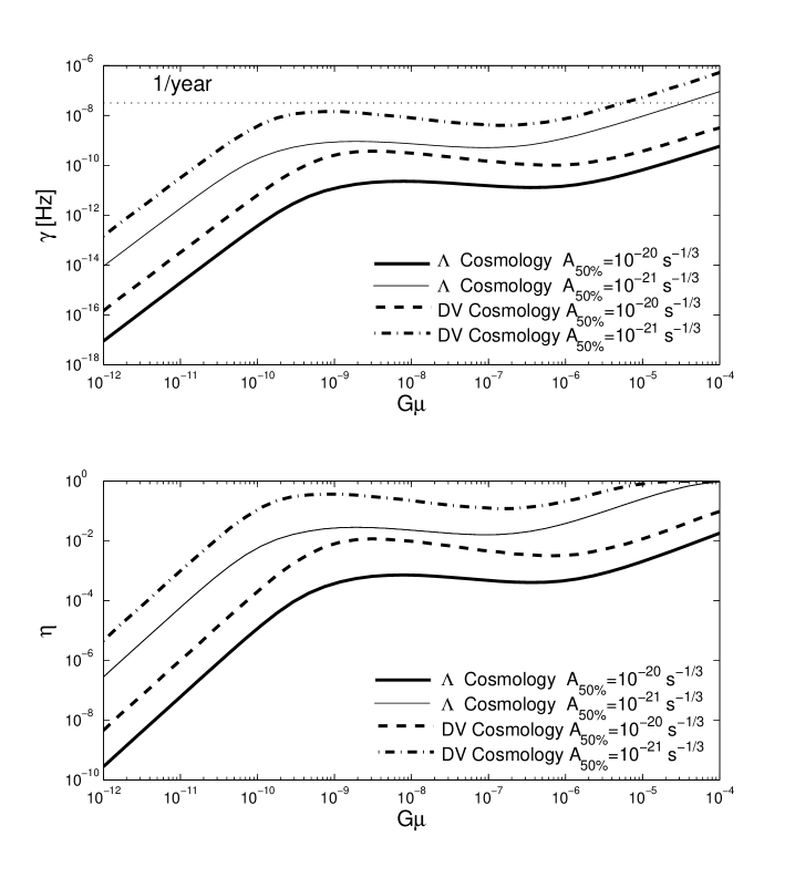
Figure 1: Plot of the rate of gravitational wave bursts, $\gamma$ (top panel), and the probability $\eta$ of having at least least one event in our data set with amplitude larger than $A_{50\%}$ in a year of observation (bottom panel), as a function of $G\mu$. For all curves we have set $\alpha=\Gamma G\mu$, $\Gamma=50$, $f_{*}=75$ Hz, $c=p=1$, and the ignorance constants $g_{1}=g_{2}=1$. The dash-dot and dashed curves show $\gamma$ and $\eta$ computed with the Damour-Vilenkin cosmological functions Eqs. (62), (63) and (64), with $A_{50\%}=10^{-21}$ s^-1/3, and $A_{50\%}=10^{-20}$ s^-1/3 respectively. The thick and thin solid curves show $\gamma$ and $\eta$ computed in a universe with a cosmological constant with amplitudes $A_{50\%}=10^{-20}$ s^-1/3, and $A_{50\%}=10^{-21}$ s^-1/3 respectively.

Figure 1 shows the rate of burst events, $\gamma$, as well as the probability $\eta$ of having at least least one event in our data set with amplitude larger than $A_{50\%}$ for a year of observation, as a function of $G\mu$ for two different models. For all curves we have set $\alpha=\Gamma G\mu$, $\Gamma=50$, $f_{*}=75$ Hz, $c=p=1$, and the ignorance constants $g_{1}=g_{2}=1$. We will refer to string models with these parameters as “classic”, which is appropriate for field theoretic strings with loops of size $l=\Gamma G\mu t$. The dashed-dot and dashed curves of Fig. 1 show $\gamma$ and $\eta$ computed using the Damour-Vilenkin cosmological functions namely, Eqs. (62), (63) and (64). For the dashed-dot curves we have used an amplitude estimate of $A_{50\%}=10^{-21}$ s^-1/3. This amplitude estimate can be obtained using the Initial LIGO sensitivity curve, setting the SNR threshold to $1$, and assuming all cusp events are optimally oriented (as used for the dashed horizontal lines of Fig. 1 in DV1 ). This is also our estimate for the amplitude in the case of Advanced LIGO. The dashed curves show $\gamma$ and $\eta$ computed with the amplitude $A_{50\%}=10^{-20}$ s^-1/3, which we feel is more appropriate for Initial LIGO. The thick and thin solid curves show $\gamma$ and $\eta$ computed by evaluating the cosmological functions (Eqs. (86), (88) and (90)) numerically for the $\Lambda$ universe (see Appendix A). The thick solid curves correspond to our amplitude estimate for Initial LIGO, and the thin solid curves to our estimate for Advanced LIGO.

The functional dependence of the rate of gravitational wave bursts on $G\mu$ is discussed in detail in Appendix B. Here we summarise those findings. From left to right, the first steep rise in the rates as a function of $G\mu$ of the dashed and dashed-dot curves of Fig. 1 comes from events produced at small redshifts ($z\ll 1$). The peak and subsequent decrease in the rate starting around $G\mu\sim 10^{-9}$ comes from events produced at larger redshifts but still in the matter era ($1\ll z\ll z_{eq}$). The final rise comes from events produced in the radiation era ($z\gg z_{eq}$).

For “classic” cosmic strings ($p=\varepsilon=n=1$), the matter era maximum in our estimate for the rate of events at Initial LIGO sensitivity is about $7\times 10^{-4}$ events per year, which is substantially lower than the rate $\sim 1$ per year suggested by the results of Damour and Vilenkin DV2 ; DV0 ; DV1 . The bulk of the difference arises from our estimate of a detectable amplitude. This is illustrated by the dashed-dot and dashed curves of Fig. 1, which use the same cosmological functions, and two estimates for the amplitude, $A_{50\%}=10^{-21}$ s^-1/3 and $A_{50\%}=10^{-20}$ s^-1/3 respectively. Our amplitude estimate results in a decrease in the burst rate by about a factor of $100$ at the matter era peak. A more detailed discussion of the effect of the amplitude on the rate can be found in Appendix B. The remaining discrepancy arises from differences in the cosmology, as well as factors of $O(1)$ that were dropped in the previous estimates, which account for a further decrease by factor of about $10$. This is illustrated by the difference between the dashed-dot and thin solid curves of Fig. 1, which use the same amplitude estimate $A_{50\%}=10^{-21}$ s^-1/3, and the Damour-Vilenkin cosmological interpolating functions (Eqs. (62), (63) and (64)) and the $\Lambda$ universe functions (Eqs. (86), (88) and (90)) respectively. When $z<<1$, the effects of a cosmological constant are un-important and differences arise from factors of $O(1)$ that were dropped in the previous estimates. For $z\gtrsim 1$, the differences arise from a combination of the effects of a cosmological constant as well as factors of $O(1)$. The net effect is that the chances of seeing an event from “classic” strings using Initial LIGO data have dropped from order unity to about $10^{-3}$ at the matter era peak. This is illustrated by the difference between the dashed-dot and thick solid curves of Fig. 1. The dashed-dot curves were computed using the amplitude estimate $A_{50\%}=10^{-21}$ s^-1/3 and the Damour-Vilenkin interpolating cosmological functions, whereas the thick solid curves use an amplitude estimate of $A_{50\%}=10^{-20}$ s^-1/3 in the $\Lambda$ universe.

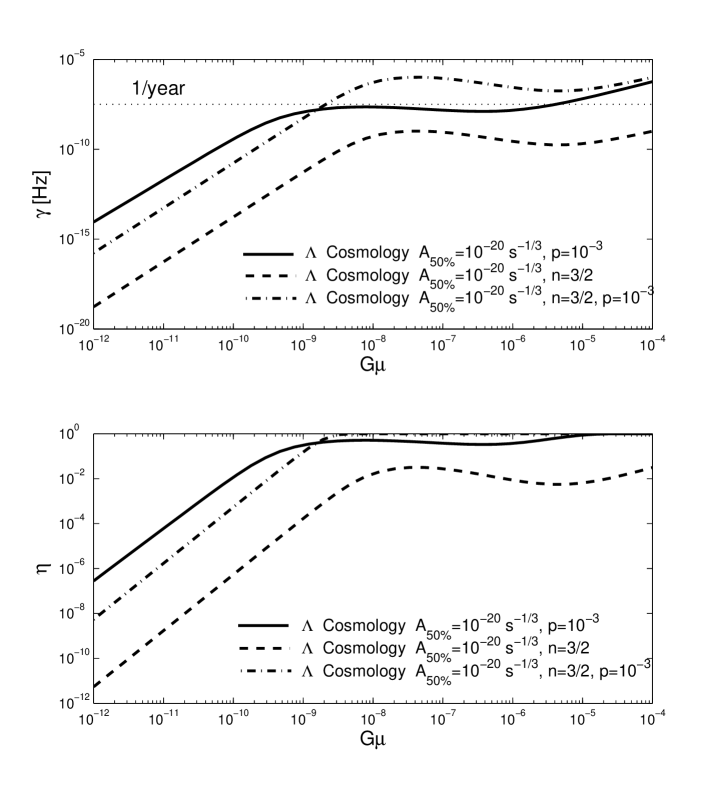
Figure 2: Comparison of $\gamma$ (top panel) and $\eta$ with a year of observation (bottom panel), as a function of $G\mu$ for several string models. For all three curves an Initial LIGO amplitude estimate of $A_{50\%}=10^{-20}$ s^-1/3 has been used, and the cosmological functions have been evaluated in the $\Lambda$ universe. The model parameters are identical to those of Fig. 1 except where indicated. The solid curves show $\gamma$ and $\eta$ computed with a reconnection probability of $p=10^{-3}$. The dashed curves show $\gamma$ and $\eta$ computed with a size of loops given by Eq. (57) with $\varepsilon=1$, and $n=3/2$. The dashed-dot curves show the combined effect of a low reconnection probability, $p=10^{-3}$, as well as a size of loops given by Eq. (57) with $\varepsilon=1$, and $n=3/2$.

Cosmic superstrings, however, may still be detectable by Initial LIGO. Furthermore, if the size of the small-scale structure is given by gravitational back-reaction, reasonable estimates for what the size of loops might be also lead to an enhanced rate of bursts. Figure 2 illustrates this point. All curves use the Initial LIGO amplitude estimate of $A_{50\%}=10^{-20}$ s^-1/3, and the cosmological functions Eqs. (86), (88) and (90) computed in the $\Lambda$ universe. The solid curves show $\gamma$ and $\eta$ computed with a reconnection probability of $p=10^{-3}$. The dashed curves show $\gamma$ and $\eta$ computed for loops with a size given by Eq. (57) with $\varepsilon=1$, and $n=3/2$. This is the value of $n$ we expect when the spectrum of perturbations on long strings is inversely proportional to the mode number, and the result we expect if the spectrum of perturbations on long strings is dominated by the largest kink trio . The dashed-dot curves show the combined effect of a low reconnection probability, $p=10^{-3}$, as well as a size of loops given by Eq. (57) with $\varepsilon=1$, and $n=3/2$. The remaining parameters for all three curves are identical to those of Fig. 1. Advanced LIGO has a considerably larger chance of making a detection of cosmic superstrings or field-theoretic strings if loops are small. This is illustrated in Fig. 3 which shows the same string models shown in Fig. 2, with our Advanced LIGO amplitude estimate of $A_{50\%}=10^{-21}$ s^-1/3.

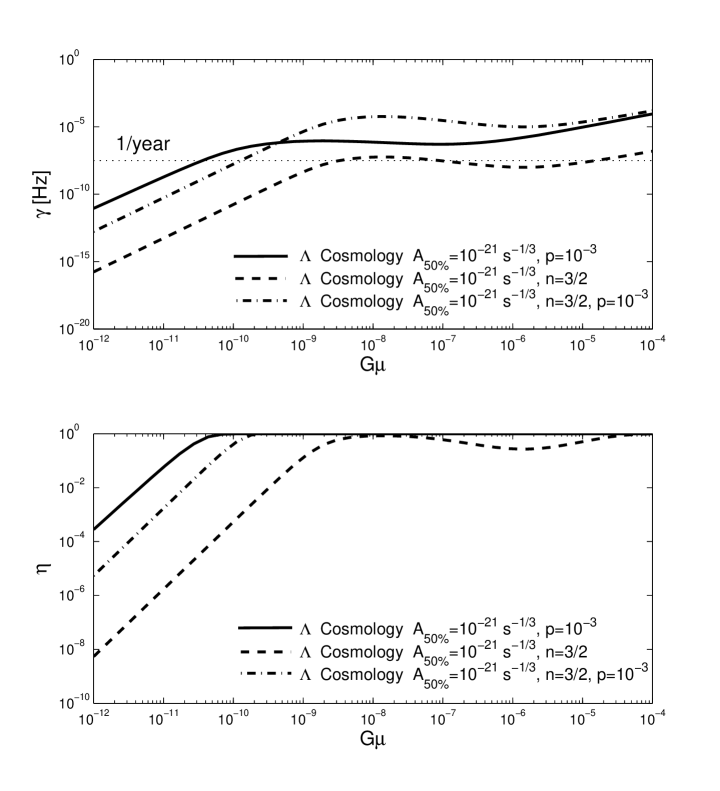
Figure 3: Same as Fig. 2 but with the Advanced LIGO amplitude estimate of $A_{50\%}=10^{-21}$ s^-1/3.

To summarise, we find the chances of detecting “classic” strings to be significantly smaller than previous estimates suggest. Even Advanced LIGO only has a few percent chance of detecting “classic” strings at the matter era peak (see the thin solid line around $G\mu\sim 10^{-9}$ in Fig. 1), though it has a good chance of detecting cosmic superstrings and cosmic strings with small loops as show in Fig. 3. Initial LIGO requires the small reconnection probability of cosmic superstrings and/or small loops to attain a reasonable chance of detection. It should be pointed out that the “classic” string model may well be incorrect. If loop sizes are given by gravitational back reaction then a reasonable guess for the spectrum of perturbations on long strings leads to $n=3/2$. This value, as shown on Fig. 2 has a substantially larger chance of detection by Initial LIGO. The size of loops, however, may not determined by gravitational back-reaction after all.

V.2 Large loops

Recent simulations RSB ; shellardrecentsim ; VOV suggest that loops are produced at sizes unrelated to the gravitational back-reaction scale. One of the simulation groups RSB finds a power law for the loop distribution, while the other two groups shellardrecentsim ; VOV find loops produced at a fixed fraction of the horizon, with loop production functions peaking around $\alpha\approx 10^{-3}$ shellardrecentsim , and the significantly larger $\alpha\approx 0.1$ VOV . It should be pointed out that the first two results RSB ; shellardrecentsim are expanding universe simulations, whereas the results of the third group VOV come from simulations in Minkowski space.

Following formation, the length of loops shrinks due to gravitational wave emission according to alexbook ,

$$l(t)=l_{i}-\Gamma G\mu(t-t_{i}),$$ (66)

where $l_{i}=\alpha t_{i}$, is the initial length, and $t_{i}$ is the time of formation of the loop. The length goes to zero at time

$$t_{f}=\left(\frac{\alpha}{\Gamma G\mu}+1\right)t_{i}.$$ (67)

Loops are long-lived when $t_{f}\gg t_{i}$, i.e. when $\alpha/(\Gamma G\mu)\gg 1$. For $\alpha\approx 0.1$, using $\Gamma=50$ the lifetime of loops is long provided $G\mu\ll 2\times 10^{-3}$, which covers the entire range of astrophysically interesting values of $G\mu$. On the other hand, if we take $\alpha\approx 5\times 10^{-4}$, then loops are long-lived only when $G\mu\ll 10^{-5}$.

If the size of loops is given by gravitational back reaction, then $\alpha$ is given by Eq. (57), and provided $n\geq 1$ all loops are short-lived. This means we can use $n(l,t)\propto\delta(l-\alpha t)$ (as we have so far) because the loop distribution is dominated by the loops that just formed.

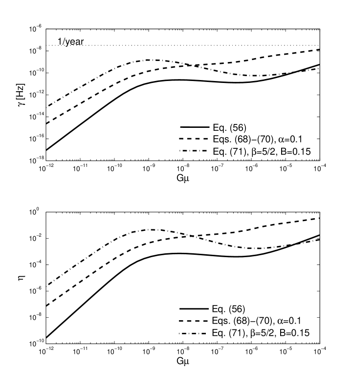
Figure 4: Plot of the rate of bursts $\gamma$ (top panel), and $\eta$, the probability of having at least least one event in our data set with amplitude larger than $A_{50\%}$ in a year of observation (bottom panel), as a function of $G\mu$ for various loops distributions. For all curves we have set $\Gamma=50$, $f_{*}=75$ Hz, $c=p=1$, and the ignorance constants $g_{1}=g_{2}=1$. As a reference we again show $\gamma$ and $\eta$ computed using the loop distribution from Eq. (56), according to Eq. (59), in the $\Lambda$-universe with $\alpha=\Gamma G\mu$ using the solid curve. The remaining curves have been computed through Eqs. (55) and (38) with $A_{50\%}=10^{-20}$ s^-1/3. The dashed curves show $\gamma$ and $\eta$ computed using the loop distribution of Eqs. (68), (69), and (70). The dashed-dot curves show $\gamma$ and $\eta$ computed with Eq. (71).

If loops are long-lived, the distribution can be calculated if a scaling process is assumed (see alexbook , §9.3.3 and §10.1.2). In the radiation era it is

$$n(l,t) = \chi_{r}t^{-3/2}(l+\Gamma G\mu t)^{-5/2},$$ (68)

$$l<\alpha t,\,\,\,t<t_{\text{eq}}$$

where $\chi_{r}\approx 0.4\zeta\alpha^{1/2}$, and $\zeta$ is a parameter related to the correlation length of the network found in numerical simulations of radiation era evolution to be about $15$ (see Table 10.1 in alexbook ). The upper bound on the length arises because no loops are formed with sizes larger than $\alpha t$.

In the matter era the distribution has two components, loops formed in the matter era and survivors from the radiation era. Loops formed in the matter era have lengths distributed according to,

$$n_{1}(l,t) = \chi_{m}t^{-2}(l+\Gamma G\mu t)^{-2},$$ (69)

$$\alpha t_{\text{eq}}-\Gamma G\mu(t-t_{\text{eq}})<l<\alpha t,\,\,\,t>t_{\text{eq}}$$

with $\chi_{m}\approx 0.12\zeta$, with $\zeta\approx 4$ (see Table 10.1 in alexbook ). The lower bound on the length is due to the fact that the smallest loops present in the matter era started with a length $\alpha t_{eq}$ when they were formed and their lengths have since decreased due to gravitational wave emission. Additionally there are loops formed in the radiation era that survive into the matter era. Their lengths are distributed according to,

$$n_{2}(l,t) = \chi_{r}t_{\text{eq}}^{1/2}t^{-2}(l+\Gamma G\mu t)^{-5/2},$$ (70)

$$l<\alpha t_{\text{eq}}-\Gamma G\mu(t-t_{\text{eq}}),\,\,\,t>t_{\text{eq}},$$

where the upper bound on the length comes from the fact that the largest loops formed in the radiation era had a size $\alpha t_{eq}$ but have since shrunk due to gravitational wave emission.

The simulations in RSB find a power law for the loop distribution, $n(l)\propto l^{-\beta}$. If all loops produced are long-lived, meaning no loops are produced with sizes below $\Gamma G\mu t$, the distribution we expect is

$$n(l,t)=Bt^{\beta-4}(l+\Gamma G\mu t)^{-\beta}.$$ (71)

The most recent fits to their loop distribution find $\beta\approx 5/2$, in both the radiation and matter eras, and $B\approx 0.1,0.2$ in the matter and radiation eras respectively Rprivate .

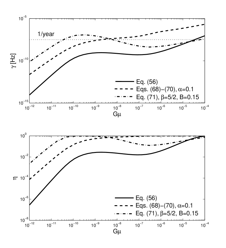
Figure 5: Same as Fig. 4 but using our Advanced LIGO amplitude estimate $A_{50\%}=10^{-21}$ s^-1/3.

We can use the results of Sec. IV to compute the rate of bursts for these loop distributions. Figure 4 shows the burst rate $\gamma$, and the probability $\eta$ of having at least least one event in our data set with amplitude larger than $A_{50\%}$ in a year of observation as a function of $G\mu$ for all the above distributions. For all curves we have set $\Gamma=50$, $f_{*}=75$ Hz, $c=p=1$, and the ignorance constants $g_{1}=g_{2}=1$. We have evaluated the cosmological functions in the $\Lambda$ universe. As a reference, we again show $\gamma$ and $\eta$ computed using the loop distribution from Eq. (56), according to Eq. (59), with $\alpha=\Gamma G\mu$ using the solid curves. The remaining curves have been computed through Eqs. (55) and (38) with $A_{50\%}=10^{-20}$ s^-1/3. The dashed curves show $\gamma$ and $\eta$ computed using the loop distribution of Eqs. (68), (69), and (70) with $\alpha=0.1$. The dashed-dot curves show $\gamma$ and $\eta$ computed with Eq. (71), where we have taken $\beta=5/2$, and $B=0.15$ as an approximation for both the radiation and matter eras. Figure 5 shows the same loop distributions as Fig. 4 but using our Advanced LIGO amplitude estimate $A_{50\%}=10^{-21}$ s^-1/3.

The loop distributions shown here lead to a significant enhancement in the rate. Note that we have not included the enhancement in the rate of bursts for the case of cosmic superstrings $p<1$. Given the range of results, it is important to determine whether the loop sizes at formation are determined by gravitational back-reaction, or whether they are large and we require a revised loop distribution.

VI Results II: Constraints

If no events can be positively identified in a search, we can use the results of Sec. III to constrain the parameter space of theories that lead to the production of cosmic strings. Unfortunately, as we have mentioned, considerable uncertainties remain in models of cosmic string evolution. Nevertheless, we can place constraints that are correct in the context of a particular string model. Here we will illustrate the procedure for the loop distribution, Eq. (56), and the resulting rate Eq. (59).

We would like to absorb the ignorance constants $g_{1}$ and $g_{2}$ into the parameters of the model. The two ignorance constants enter the expression for the rate Eq. (59) in three ways. First, they affect the upper limit of the integral Eq. (61) through Eq. (60), which is,

$$\frac{\varphi^{2/3}_{t}(z)}{(1+z)^{1/3}\varphi_{r}(z)}=\frac{AH^{-1/3}_{0}}{g_{1}G\mu\alpha^{2/3}}.$$ (72)

Secondly, they enter through $\theta_{m}$ in the theta function cutoff of the rate,

$$\theta_{m}=(g_{2}(1+z)f_{*}\alpha H_{0}^{-1}\varphi_{t}(z))^{-1/3},$$ (73)

and finally, the rate itself (Eq. (59)) is proportional to $g_{2}^{-2/3}$.

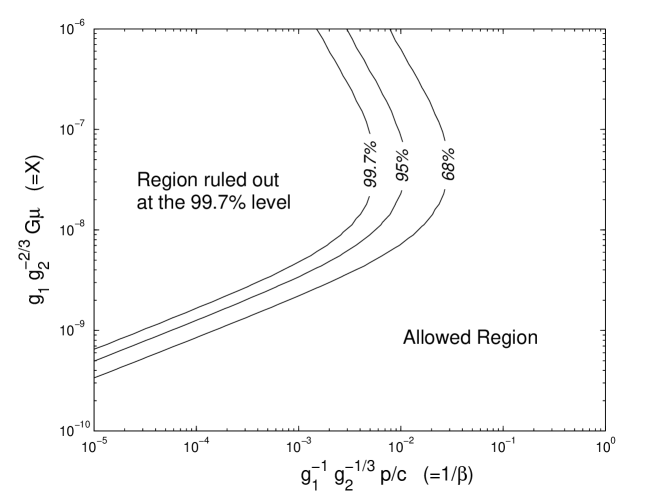
Figure 6: Contour of excluded regions at various confidences. In the cosmic string model we have set $\tilde{\varepsilon}=1$, and $n=3/2$, and allowed $X$ and $\beta$ to vary. For the loudest event we have used our Initial LIGO estimate for the amplitude $A_{50\%}=10^{-20}$ s^-1/3.

If we write $\alpha=\varepsilon(\Gamma G\mu)^{n}$, and substitute into Eqs. (73) and (72), we can simultaneously absorb $g_{1}$ and $g_{2}$ into new variables $\tilde{\varepsilon}(\varepsilon,g_{1},g_{2},n)$ and $X(G\mu,g_{1},g_{2})$. Looking at Eq. (73) we can write an identity for the ignorance constants and the variables we want to absorb them into,

$$g_{2}\varepsilon(\Gamma G\mu)^{n}=\tilde{\varepsilon}(\Gamma X)^{n}.$$ (74)

Similarly, looking at the denominator of the right hand side of Eq. (72) we write,

$$g_{1}G\mu[\varepsilon(\Gamma G\mu)^{n}]^{2/3}=X[\tilde{\varepsilon}(\Gamma X)^{n}]^{2/3}$$ (75)

These equations can be simultaneously solved to give,

$$G\mu=g^{-1}_{1}g_{2}^{2/3}X,$$ (76)

and

$$\varepsilon=g^{n}_{1}g_{2}^{-2n/3-1}\tilde{\varepsilon}.$$ (77)

If we replace $G\mu$ by Eq. (76) and $\varepsilon$ by Eq. (77), in Eq. (73) we obtain,

$$\theta_{m}=((1+z)f_{*}\tilde{\varepsilon}(\Gamma X)^{n}H_{0}^{-1}\varphi_{t}(z))^{-1/3},$$ (78)

and if we make the same replacements into Eq. (72),

$$\frac{\varphi^{2/3}_{t}(z)}{(1+z)^{1/3}\varphi_{r}(z)}=\frac{AH^{-1/3}_{0}}{X(\tilde{\varepsilon}(\Gamma X)^{n})^{2/3}},$$ (79)

namely, we obtain functions of $\tilde{\varepsilon}$ and $X$ only.

Finally, if we replace $G\mu$ by Eq. (76) and $\varepsilon$ by Eq. (77), in our expression for the rate, Eq. (59), we see that we can absorb the remaining factors by defining a quantity,

$$\beta=g_{2}^{1/3}g_{1}\frac{c}{p}.$$ (80)

This yields a rate,

$$\frac{dR}{dz} = H_{0}\frac{\beta(f_{*}H^{-1}_{0})^{-2/3}}{2(\tilde{\varepsilon}(\Gamma X)^{n})^{5/3}\Gamma X}\varphi^{-14/3}_{t}(z)\varphi_{V}(z)(1+z)^{-5/3}$$ (81)

$$\times \Theta(1-\theta_{m}),$$

where $\theta_{m}$ given by Eq. (78). The parameters that we constrain are now $X$, $n$, $\tilde{\varepsilon}$, and $\beta$.

Figure 6 illustrates the application of this procedure. We show a contour plot constructed by computing the rate and comparing it to $\gamma_{68\%}\approx 1.14/T$, $\gamma_{95\%}\approx 3.00/T$ and $\gamma_{99.7\%}\approx 5.81/T$. In the cosmic string model we have set $\tilde{\varepsilon}=1$, and $n=3/2$, and allowed $X$ and $\beta$ to vary. In place of the loudest event we have used our Initial LIGO estimate for the amplitude $A_{50\%}=10^{-20}$ s^-1/3. If we set the ignorance constants to unity, and $c=1$, we see that for $G\mu$ in the range $4\times 10^{-9}-10^{-6}$, values of the reconnection probability around $p=10^{-3}$ are ruled out at the $99.7\%$ level.

It is interesting to note that for cosmic superstrings a bound on the reconnection probability might be turned into a bound on the string coupling and/or a bound on the size of extra dimensions.

VII Summary and Conclusions

We begun this work by considering the data analysis infrastructure necessary to perform a search for gravitational waves from cosmic (super)string cusps. The optimal method to use in such a search is matched-filtering. We have described the statistical properties of the matched-filter output, a method for template bank construction, and an efficient algorithm to compute the matched-filter. When data from multiple interferometers is available, we discussed consistency checks that can be used to greatly reduce the false alarm rate.

The relevant output of the matched-filter is the estimated signal amplitude. We have shown that in a search, the event with the largest amplitude can be used to to set upper limits on the rate via the loudest event method. The upper limit depends on the cosmological rate of events and the efficiency, which can be computed using simulated signal injections into the data stream. The injections should account for certain properties of the population, such as the frequency distribution ($dR/df\propto f^{-5/3}$ for cusps), and source sky locations. We have briefly discussed the related issue of sensitivity, which also depends on the search detection efficiency, as well as background estimation. We have made a single estimate for the amplitude of detectable and loudest events using the Initial LIGO design curve and an SNR threshold $\rho_{\text{th}}=4$, which we believe is a reasonable operating point for a pipeline. Assuming that there are no significant inefficiencies in the pipeline, that the rate of false alarms is sufficiently low, and that no signals or instrumental glitches are present in the final trigger set, we expect this amplitude to be $A_{50\%}\approx 10^{-20}$s^-1/3. Advanced LIGO is expected to be an order of magnitude more sensitive then Initial LIGO, so for Advanced LIGO we expect $A_{50\%}\approx 10^{-21}$s^-1/3.

We have computed the rate of bursts in the case of an arbitrary cosmic string loop distribution, using a generic cosmology. Motivated by the data analysis, we cast the rate as a function of the amplitude. We have applied this formalism in the case of a flat universe with matter, radiation and a cosmological constant, to the loop distribution used in the estimates of DV2 ; DV0 ; DV1 . For the “classic” (field theoretic strings with loops of size $l=\Gamma G\mu t$) model of cosmic strings considered in DV0 ; DV1 , we find substantially lower event rates than their estimates suggest. The bulk of the difference arises from our estimate of a detectable amplitude. The effect of the amplitude estimate on the rate is discussed in detail in Appendix B. The remaining discrepancy arises from differences in the cosmology (the cosmological model in DV2 ; DV0 ; DV1 included only matter and radiation), as well as factors of $O(1)$ that were dropped in the previous estimates. The net effect is that the chances of seeing an event from “classic” strings using Initial LIGO data have dropped from order unity to about $10^{-3}$ at the local maximum of the rate (which comes from bursts produced in the matter era). This result is illustrated in Fig. 1.

The “classic” string model may well be incorrect so these results are not necessarily discouraging. Two new results indicate that this is the case.

Recently it was realised that damping of perturbations propagating on strings due to gravitational wave emission is not as efficient as previously thought KandIGW . As a consequence, the size of the small-scale structure is sensitive the spectrum of perturbations present on the strings, and can be much smaller than the canonical value $\Gamma G\mu t$ trio . If the size of loops is given by gravitational back-reaction, a reasonable guess for the spectrum of perturbations on long strings leads to

$$\alpha\sim\left(\Gamma G\mu\right)^{3/2},$$ (82)

which in turn could lead to detectable events by Advanced LIGO, or Initial LIGO if we are dealing with cosmic superstrings. This is illustrated in Figs. 2 and  3.

Even more recently, simulations RSB ; shellardrecentsim ; VOV suggest that loops are produced at sizes unrelated to the gravitational back-reaction scale, $\alpha\lesssim 1$. In this case loops of many different sizes are present at any given time (because they are very long-lived), and the use of a revised loop distribution becomes necessary. The particulars of the distribution are currently under debate, but all distributions currently considered lead to an enhanced rate of bursts relative to the “classic” model. Results for the rate for various loop distributions are shown in Figs. 4 and 5.

Finally, we have have shown how the parameter space of theories that lead to the production of cosmic strings might be constrained in the absence of a detection. Results for a model of cosmic superstrings, where the loop size is given by Eq. (82), are shown in Fig. 6. Initial LIGO may yield interesting constraints on the reconnection probability for some range of string tensions. Intriguingly, a bound on the reconnection probability might be turned into a bound on the string coupling and/or a bound on the size of extra dimensions, in the case of cosmic superstrings.

Wish list

Unfortunately, there remain considerable uncertainties in models of cosmic string evolution. While we can estimate the detectability, and place constraints, that are correct in the context of a particular string model, the current parameter space allows for a wide spectrum of burst rates in the interesting range of string tensions.

We would like to finish by posing a set of questions to the various cosmic string simulation groups which, from the perspective of gravitational wave detection, would greatly improve predictability.

They are:

• What is the size of cosmic string loops? Are they large when they are formed, so we need to consider a loop distribution? If so, what is that distribution? Is their size instead given by gravitational back-reaction? If so, what is the spectrum of perturbations on long strings?

• What is the number of cusps per loop oscillation? Is it independent of the loop size?

• What is the size of cusps? In particular, what fraction of the loop length $l$ is involved in the cusp?

• What are the effects of low reconnection probability? In particular, what is the enhancement in the loop density that results?

Appendix A Cosmological Functions

To derive exact expressions for $\varphi_{t}(z)$, $\varphi_{r}(z)$, and $\varphi_{V}(z)$, we begin with the evolution of the Hubble function. The Hubble function is given by

$$H(z)=H_{0}h(z),$$ (83)

with, for a flat universe,

$$h(z)=\left(\Omega_{m}(1+z)^{3}+\Omega_{r}(1+z)^{4}+\Omega_{\Lambda}\right)^{1/2}.$$ (84)

Here, $\Omega_{i}=\rho_{i}(z=0)/\rho_{c}(z=0)$ is the present energy density of the i’th component, relative to the critical density. The subscripts $m$, $r$, and $\Lambda$ stand for matter (dark and baryonic), radiation, and the cosmological constant, respectively. Since we assume the universe flat, $\Sigma\Omega_{i}=1$.

We will use the set of cosmological parameters in stdcosmoref , which provide a good fit to recent cosmological data. The precise values of the parameters are not critical, but we include them here for clarity. They are, $H_{0}=73$ km s^-1Mpc${}^{-1}=2.4\times 10^{-18}$ s^-1, $\Omega_{m}=0.25$, $\Omega_{r}=4.6\times 10^{-5}$, and $\Omega_{\Lambda}=1-\Omega_{m}-\Omega_{r}$.

To compute the relation between the time and the redshift, we use the fact that $dz/dt=-(1+z)H$, and write

$$t = \int_{0}^{t}dt^{\prime}=\int_{z}^{\infty}\frac{dz^{\prime}}{(1+z^{\prime})H(z^{\prime})}.$$ (85)

The dimensionless function $\varphi_{t}(z)$ of Eq. (44) is thus,

$$\varphi_{t}(z)=\int_{z}^{\infty}\frac{dz^{\prime}}{(1+z^{\prime})h(z^{\prime})}.$$ (86)

In order to compute the amplitude distance DV1 as a function of the redshift, we consider null geodesics in an FRW universe. We can take the polar and azimuthal coordinates to be constant and let the radial coordinate, $r$, vary. In this case we have that $dr/dt=-(1+z)$, and thus $dr/dz=1/H$. So we write

$$r=\int_{0}^{r}dr^{\prime}=\int_{0}^{z}\frac{dz^{\prime}}{H(z^{\prime})}.$$ (87)

We can therefore express the dimensionless function of Eq. (47), $\varphi_{r}(z)$, as

$$\varphi_{r}(z) = \int_{0}^{z}\frac{dz^{\prime}}{h(z^{\prime})}.$$ (88)

Finally, we would like to derive an expression for the differential volume as a function of the redshift, $dV/dz$. The differential volume element is given by

$$dV = a^{3}(t)r^{2}dr\,\sin\theta d\theta\,d\phi~{},$$

where $a(t)$ is the scale factor. Integrating over the polar and azimuthal coordinates and using $dr/dz$ gives

$$dV=4\pi a^{3}(t)r^{2}dr = \frac{4\pi r^{2}}{(1+z)^{3}H(z)}dz~{}.$$ (89)

Using Eqs. (83) and (87) gives the dimensionless function of Eq. (54)

$$\varphi_{V}(z)=\frac{4\pi\varphi_{r}^{2}(z)}{(1+z)^{3}h(z)}.$$ (90)

Appendix B Approximate analytic expression for the rate

In this appendix we compute an approximate expression for the rate as a function of the amplitude can be obtained using the interpolating functions introduced in DV2 ; DV0 ; DV1 , Eqs. (62), (63), and (64). The result is useful to understand the qualitative behaviour of the rate curves shown in Figs. 1, 2, and 3.

Using Eqs. (46) and (63) we can write the amplitude of an burst from a loop of length $l$ at a redshift $z$ as

$$A\sim\frac{G\mu l^{2/3}(1+z)^{2/3}}{t_{0}z}.$$ (91)

We take the size of the feature that produces the cusp to be the typical size of loops, $l(z)=\alpha H^{-1}_{0}\varphi_{t}(z)$, with $\varphi_{t}(z)$ given by Eq. (62), so that,

$$A\sim G\mu\alpha^{2/3}t_{0}^{-1/3}z^{-1}(1+z)^{-1/3}(1+z/z_{eq})^{-1/3}.$$ (92)

We define a dimensionless amplitude $a$,

$$a\equiv\frac{A}{G\mu\alpha^{2/3}t_{0}^{-1/3}}\sim z^{-1}(1+z)^{-1/3}(1+z/z_{eq})^{-1/3}$$ (93)

Depending on the value of $z$, the function $a(z)$ has three different asymptotic behaviours,

$$a(z)\sim\left\{\begin{array}[]{ccc}z^{-1}&z\ll 1\\ z^{-4/3}&1\ll z\ll z_{eq}\\ z_{eq}^{1/3}z^{-5/3}&z\gg z_{eq}\end{array}\right.$$ (94)

The regime where $z\ll 1$ corresponds to cusp events occurring nearby, the regime where $1\ll z\ll z_{eq}$ corresponds to matter-era events, and the regime where $z\gg z_{eq}$ corresponds to radiation era events.

At $z=1$, we define

$$a_{1}\equiv a(z=1)\approx 2^{-1/3}\sim 1,$$

and at $z=z_{eq}$,

$$a_{eq}\equiv a(z=z_{eq})\approx z_{eq}^{-4/3}2^{-1/3}\approx z_{eq}^{-4/3}a_{1}\approx 4\times 10^{-6}.$$

This means we can write,

$$z_{eq}\sim a_{eq}^{-3/4}.$$ (95)

The regime where $z\ll 1$, corresponds to $a\gg 1$; the regime where $1\ll z\ll z_{eq}$, corresponds to $a_{eq}\ll a\ll 1$; and the regime where $z\gg z_{eq}$, corresponds to $a\ll a_{eq}$. This means that we can write,

$$z(a)\sim\left\{\begin{array}[]{ccc}a_{eq}^{-3/20}a^{-3/5}&a\ll a_{eq}\\ a^{-3/4}&a_{eq}\ll a\ll 1\\ a^{-1}&a\gg 1\end{array}\right.$$ (96)

We can write this in terms of the interpolating function,

$$z(a)\sim a_{eq}^{-3/20}a^{-3/5}\left(1+\frac{a}{a_{eq}}\right)^{-3/20}\left(1+a\right)^{-1/4}.$$ (97)

Using Eqs. (62) and (64), we can write the rate of events as a function of the redshift, Eq. (59), as,

$$\frac{dR}{dz}\sim bz^{2}(1+z)^{-7/6}(1+z/z_{eq})^{11/6},$$ (98)

where $b$ is defined as

$$b\equiv 10^{2}c\alpha^{-5/3}(p\Gamma G\mu)^{-1}t_{0}^{-1}(f_{*}t_{0})^{-2/3},$$ (99)

and the theta-function cutoff has been ignored for convenience. In the three regimes considered above the rate is given by,

$$dR\sim b\times\left\{\begin{array}[]{ccc}z^{2}dz&z\ll 1\\ z^{5/6}dz&1\ll z\ll z_{eq}\\ z_{eq}^{-11/6}z^{8/3}dz&z\gg z_{eq}\end{array}\right.$$ (100)

In the regime where $z\ll 1$, corresponds to $a\gg 1$, and $z\sim a^{-1}$. This means,

$$dR\sim bz^{2}dz=ba^{-2}\frac{dz}{da}da.$$ (101)

Since,

$$\frac{dz}{da}\sim-a^{-2},$$ (102)

we have that

$$\begin{array}[]{ccc}dR\sim-ba^{-4}da,&\,\text{for}&a\gg 1.\\ \end{array}$$ (103)

The regime where $1\ll z\ll z_{eq}$, corresponds to $a_{eq}\ll a\ll 1$, and $z\sim a^{-3/4}$. This means,

$$dR\sim bz^{5/6}dz=ba^{-5/8}\frac{dz}{da}da.$$ (104)

Since,

$$\frac{dz}{da}\sim-\frac{3}{4}a^{-7/4},$$ (105)

we have that

$$\begin{array}[]{ccc}dR\sim-\frac{3}{4}ba^{-19/8}da,&\,\text{for}&a_{eq}\ll a\ll 1.\\ \end{array}$$ (106)

Finally, the regime where $z\gg z_{eq}$, corresponds to $a\ll a_{eq}$, and $z\sim(a_{eq}/a_{1})^{-3/20}a^{-3/5}$. Thus, using Eq. (95),

$$dR\sim bz_{eq}^{-11/6}z^{8/3}dz=ba_{eq}^{39/40}a^{-8/5}\frac{dz}{da}da.$$ (107)

Since,

$$\frac{dz}{da}\sim-\frac{3}{5}a_{eq}^{-3/20}a^{-8/5},$$ (108)

we have that

$$\begin{array}[]{ccc}dR\sim-\frac{3}{5}ba_{eq}^{33/40}a^{-16/5}da,&\,\text{for}&a\ll a_{eq}.\\ \end{array}$$ (109)

Summarising,

$$\frac{dR(a)}{da}\sim-b\times\left\{\begin{array}[]{ccc}a_{eq}^{33/40}a^{-16/5}&a\ll a_{eq}\\ a^{-19/8}&a_{eq}\ll a\ll 1\\ a^{-4}&a\gg 1\end{array}\right.$$ (110)

Eq. (110) can be integrated, to give the rate of events with reduced amplitude greater than $a$,

$$R_{>a}\sim b\times\left\{\begin{array}[]{ccc}a_{eq}^{33/40}a^{-11/5}&a\ll a_{eq}\\ a^{-11/8}&a_{eq}\ll a\ll 1\\ a^{-3}&a\gg 1\end{array}\right.$$ (111)

We can determine the functional dependence of the rate for the simple case when $\alpha=\Gamma G\mu$, which we can then compare with the dashed and dashed-dot curves of Fig. 1. The factor of $b$, as defined by Eq. (99), contains a factor of $(G\mu)^{-1}$ as well as a factor of $(G\mu)^{-5/3}$ through its dependence on $\alpha$. So we take $b\propto(G\mu)^{-8/3}$. The dimensionless amplitude $a$, as defined by Eq. (93) also contains a factor of $(G\mu)^{-1}$ as well as a factor of $(G\mu)^{-2/3}$ through its dependence on $\alpha$, so that $a\propto(G\mu)^{-5/3}$.

In Eq. (111), (as we have mentioned) the regime where $a\ll a_{eq}$ maps into the radiation era, and in this case the rate,

$$R\propto G\mu.$$ (112)

The regime where $a_{eq}\ll a\ll 1$ maps into the matter era when the redshift $z\gg 1$, and the rate in this case is,

$$R\propto(G\mu)^{-31/24}.$$ (113)

The final regime when $a\gg 1$ corresponds to bursts that are coming from close by ($z\ll 1$), and the rate,

$$R\propto(G\mu)^{7/3}.$$ (114)

So we immediately see that the first steep rise in the rate as a function of $G\mu$ (from left to right) of the dashed and dashed-dot curves of Fig. 1 corresponds to bursts that are coming from small redshifts, i.e. from $z\ll 1$. The slight decrease in the rate comes from bursts produced at large redshifts, but still in the matter era, i.e. $1\ll z\ll z_{eq}$, and the final increase in the rate comes from bursts produced in the radiation era, $z\gg z_{eq}$.

Eq. (111) also makes it easy to understand the lower burst event rates we find relative to the previous estimates of Damour and Vilenkin DV2 ; DV0 ; DV1 (see the the dashed and dashed-dot curves of Fig. 1). They compared the strain produced by cosmic string burst events at a rate of 1 per year to a noise induced SNR $1$ event, given the Initial LIGO design noise curve (see, for example, the dashed lines in Fig. 1 of DV2 ). In our treatment, the amplitude that corresponds to is $A\approx 10^{-21}$s^-1/3. To make our amplitude estimate we have chosen an SNR threshold of $4$, which, as proposed in DV2 , is a reasonable operating point for a data analysis pipeline, and have included the effects of the antenna pattern of the instrument, which averages to a factor of $\sqrt{5}$. The combined effect is to increase the amplitude estimate by about a factor of $10$, to make it $A\approx 10^{-20}$s^-1/3.

Looking at Eq. (111), we see that an increase in the amplitude of a factor of $10$, results in a decrease of a factor of $10^{3}$ in the rate of nearby bursts ($z\ll 1$), a decrease by a factor of about $24$ in the rate of bursts produced in the matter era ($1\ll z\ll z_{eq}$), and a decrease by about a factor of $160$ in the rate of bursts produced in the radiation era ($z\gg z_{eq}$).

References

- (1) T.W.B. Kibble, J. Phys. A9 (1976) 1387.
- (2) A. Vilenkin and E.P.S Shellard, Cosmic strings and other Topological Defects. Cambridge University Press, 2000.
- (3) N. Jones, H. Stoica, S.H.Henry Tye, JHEP 0207 (2002) 051, hep-th/0203163.
- (4) S. Sarangi, S.H.Henry Tye, Phys.Lett.B 536 (2002) 185, hep-th/0204074.
- (5) G. Dvali, A. Vilenkin, JCAP 0403 (2004) 010.
- (6) N. Jones, H. Stoica, S.H.Henry Tye, Phys.Lett. B563 (2003) 6.
- (7) E.J. Copeland, R.C. Myers and J. Polchinski, JHEP 0406 (2004) 013.
- (8) M.G. Jackson, N.T. Jones and J. Polchinski, JHEP 0510 (2005) 013.
- (9) M. Sakellariadou, JCAP 0504 (2005) 003.
- (10) A. Avgoustidis and E.P.S Shellard, astro-ph/0512582.
- (11) T. Damour and A. Vilenkin, Phys. Rev. D71 (2005) 063510.
- (12) T. Damour and A. Vilenkin, Phys. Rev. Lett. 85 (2000) 3761.
- (13) T. Damour and A. Vilenkin, Phys. Rev. D64 (2001) 064008.
- (14) J. Polchinski, hep-th/0410082; J. Polchinski, hep-th/0412244.
- (15) E. Babichev, M. Kachelriess, Phys. Lett. B 614 (2005) 1.
- (16) X. Siemens, K.D. Olum, Phys.Rev. D68 (2003) 085017.
- (17) I.S. Gradstheyn and I.M. Ryzhyk, Table of Integrals Series and Products.
- (18) A. Albrecht and N. Turok, Phys. Rev. D40 (1989) 973; D.P. Bennett and F.R. Bouchet, Phys. Rev. D41 (1990) 2408; B. Allen and E.P.S. Shellard, Phys. Rev. Lett. 64 (1990) 119.
- (19) C. Ringeval, M. Sakellaridou and F. Bouchet, astro-ph/0511646.
- (20) C.J.A.P. Martins and E.P.S. Shellard, astro-ph/0511792.
- (21) V. Vanchurin, K.D. Olum and A. Vilenkin, gr-qc/0511159.
- (22) C. Cutler and E.E. Flanagan, Phys.Rev.D 49 (1994) 2658.
- (23) B.J. Owen, Phys.Rev.D 53 (1996) 6749.
- (24) B. Allen, W.G. Anderson, P.R. Brady, D.A. Brown and J.D.E. Creighton, gr-qc/0509116
- (25) LIGO Scientific Collaboration (B. Abbott et al.), Phys.Rev.D72 (2005) 082001.
- (26) P.R. Brady, J.D.E. Creighton and A.G. Wiseman, Class.Quant.Grav.21 (2004) S1775.
- (27) K.S. Thorne, 300 Years of Gravitation. Cambridge University Press, 1987.
- (28) A. Lazzarini, R. Weiss (1996), LIGO technical report, LIGO-E950018-02; A. Abramovici, et al. Science 256 (1992) 325; ”Proposal to the National Science Foundation – The Construction, Operation, and Supporting Research and Development of a Laser Interferometer Gravitational-Wave Observatory”, December 1989, Thorne, Drever, Weiss, amd Raab, PHY-9210038.
- (29) LIGO Scientific Collaboration (B. Abbott et al.), Phys.Rev.D69 (2004) 102001.
- (30) A. Vilenkin, private communication.
- (31) X. Siemens, K.D. Olum, Nucl.Phys.B611 (2001) 125, gr-qc/0104085.
- (32) X. Siemens, K.D. Olum, A. Vilenkin, Phys.Rev.D66 (2002) 043501, gr-qc/0203006
- (33) C. Ringeval, private communication.
- (34) S. Eidelman et al., Phys. Lett. B592, 1 (2004); A.R. Liddle and O. Lahav, astro-ph/0601168.