Bounds for scalar waves on self-similar naked-singularity backgrounds.

Abstract

The stability of naked singularities in self-similar collapse is probed using scalar waves. It is shown that the multipoles of a minimally coupled massless scalar field propagating on a spherically symmetric self-similar background spacetime admitting a naked singularity maintain finite $L^{2}$ norm as they impinge on the Cauchy horizon. It is also shown that each multipole obeys a pointwise bound at the horizon, as does its locally observed energy density. $L^{2}$ and pointwise bounds are also obtained for the multipoles of a minimally coupled massive scalar wave packet.

1 Introduction

Spacetimes admitting naked singularities provide test-beds for the cosmic censorship conjecture. Of course the mere existence of an example of a spacetime admitting a naked singularity (NS) is not evidence that the conjecture is invalid, as such spacetimes are typically unrealistic in that they possess a high degree of symmetry. Rather, the conjecture may be probed by determining whether or not these spacetimes (and their NS) are stable under perturbations. This addresses the question of whether or not NS may arise from open sets of initial data, which in turn addresses (to an extent) the question of whether or not NS may arise in nature. For example, the NS of a charged spherical black hole cannot arise in nature as it has been shown that the Cauchy horizon accompanying the singularity is unstable under small perturbations (see [1] for a review). However, there is evidence that this instability is not present for certain spherically symmetric self-similar spacetimes.

Harada and Maeda have shown the existence of perfect fluid spacetimes with a soft equation of state that admit naked singularities but which are stable under perturbations impinging on the singularity: these have been dubbed the general relativistic Larson-Penston spacetimes (GRLP) [2]. (The fate of perturbations impinging on the Cauchy horizon has not been studied, and this is an important question.) It has also been shown that individual massless scalar wave modes of the form $e^{\lambda v}\phi(x)$ remain finite in the approach to the Cauchy horizon $x\to x_{c}$ in a wide class of spherically symmetric self-similar spacetimes [3]. Here, $v$ is an advanced Bondi coordinate and $x=v/r$ is a similarity variable (see below; $r$ is the radius function of the spherically symmetric spacetime). The same has also been shown to be true for the individual modes of gravitational (metric and matter) perturbations of the self-similar Vaidya spacetime [4].

The aim of the present paper is to expand upon the second of these three points by studying the propagation of a minimally coupled, massless scalar field in self-similar spacetimes without recourse to a mode decomposition (Fourier transform). We find that the results for individual modes essentially carry over to the multipoles of the full field, and so have greater significance. (We us the term multipole to refer to the coefficients $\phi_{\ell,m}$ of the spherical harmonics in the standard angular decomposition of a scalar field $\phi$ on a spherically symmetric background: $\phi=\sum_{\ell,m}\phi_{\ell,m}Y_{\ell}^{m}(\theta,\varphi)$.) The $L^{2}$ norm of each multipole field, its pointwise values and its local energy density remain finite in the approach to the Cauchy horizon. We consider this to be evidence of the stability of such naked singularities: the scalar field can be considered to model the behaviour of gravitational perturbations of the spacetime.

In the following section, we describe the global structure of the class of spacetimes under consideration: spherically symmetric spacetimes admitting a naked singularity and whose energy momentum tensor obeys the weak energy condition. In section 3, we discuss the $L^{2}$ and local stability of a massless scalar field propagating in such a spacetime, and study the local energy density of the field in section 4. We consider massive fields in section 5, and discuss our results in section 6. We use the curvature conventions of [5], setting $G=c=1$, and use the notation of [6] for Sobolev spaces. A black square   indicates the end or absence of a proof.

2 Self-similar spherically symmetric spacetimes admitting a naked singularity.

We will consider the class of spacetimes which have the following properties. Spacetime $({\cal{M}},g)$ is spherically symmetric and admits a homothetic Killing vector field. These symmetries pick out a scaling origin ${\cal{O}}$ on the central world-line $r=0$ (which we will refer to as the axis), where $r$ is the radius function of the spacetime. We assume regularity of the axis to the past of ${\cal{O}}$ and of the past null cone ${\cal{N}}$ of ${\cal{O}}$. We will use advanced Bondi co-ordinates $(v,r)$ where $v$ labels the past null cones of $r=0$ and is taken to increase into the future. Translation freedom in $v$ allows us to situate the scaling origin at $(v,r)=(0,0)$ and identifies $v=0$ with ${\cal{N}}$. The homothetic Killing field is

$${\vec{\xi}}=v\frac{\partial}{\partial v}+r\frac{\partial}{\partial r}.$$

The line element may be written

$$ds^{2}=-2Ge^{\psi}dv^{2}+2e^{\psi}dvdr+r^{2}d\Omega^{2},$$ (1)

where $d\Omega^{2}$ is the line element of the unit 2-sphere. The homothetic symmetry implies that $G(v,r)=G(x),\psi(v,r)=\psi(x)$ where $x=v/r$. The only co-ordinate freedom remaining in (1) is then $v\to V(v)$; this is removed by taking $v$ to measure proper time along the regular center $r=0$.

We will not specify the energy-momentum tensor of $({\cal{M}},g)$, but will demand that it satisfies the null energy condition: $T_{ab}k^{a}k^{b}\geq 0$ for all null vectors $\vec{k}$. Note that this condition is implied by both the strong energy condition and the weak energy condition. A complete description of energy conditions in spherical symmetry is given in [3]. Of these, the following will be used.

$$x\psi^{\prime}\leq 0,$$ (2)

$$G^{\prime}-\psi^{\prime}(1-xG)G\leq 0.$$ (3)

We define the interior region ${\cal{M}}_{int}$ of spacetime to be the interior of ${\cal{N}}$, i.e. the interior of the causal past of ${\cal{O}}$. We demand that there are no trapped 2-spheres in ${\cal{M}}_{int}$. This is an initial regularity condition, and is equivalent to $G>0$ in ${\cal{M}}_{int}$. We also note that except for the trivial case of flat spacetime, there must be a curvature singularity at ${\cal{O}}$ [3].

The presence of a naked singularity is characterised by the following result proven in [3].

Theorem 1

There exists a future pointing radial null geodesic in ${\cal{M}}$ with past endpoint on ${\cal{O}}$ if and only if there exists a positive root of the equation $xG(x)-1=0$.  

The features above define the class of spacetimes under consideration in the remainder of this paper: $({\cal{M}},g)$ is spherically symmetric and self-similar with line element (1). There exists a naked singularity, so that there is a smallest positive root $x_{c}$ of $xG-1=0$. Then the Cauchy horizon ${\cal{H}}$ is $x=x_{c}$. We take $G,\psi$ to be analytic on $(-\infty,x_{c}]$. Einstein’s equation and the null energy condition are assumed, so that (2) and (3) apply. The corresponding conformal diagram is shown in Figure One. There are subsets of the following categories of spacetimes included in this class: (i) Vaidya spacetimes (spherically symmetric null dust); (ii) Einstein-Klein-Gordon spacetimes (spherically symmetric massless scalar field coupled to gravity); (iii) Lemaître-Tolman-Bondi spacetimes (spherically symmetric dust); (iv) perfect fluid filled spacetimes (where self-similarity enforces a linear equation of state - see [7]); (v) Einstein-$SU(2)$ spacetimes (spherically symmetric $SU(2)$ sigma model coupled to gravity - see [8]). Of these, the metric functions $G,\psi$ are explicitly available only for Vaidya spacetime, which has $\psi=0,2G=1-2\lambda x$, where $\lambda$ is a constant. A naked singularity occurs for $\lambda\in(0,1/16)$. Among the other cases, the similarity coordinate $z=t/r$ (where $t$ is proper time along the fluid flow lines in the dust and perfect fluid cases and a polar slicing time coordinate in the sigma model case) is more natural than our $x$, and a nontrivial coordinate transformation is required to determine $\psi,G$ explicitly. We emphasise however that this explicit representation is not required for the present purpose.

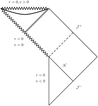
Figure 1: Conformal diagram for an example of a self-similar spacetime admitting a globally naked singularity. We use the advanced Bondi co-ordinates $v$ and $r$ described in Section 2. The Cauchy horizon is shown dashed, the event horizon as a double line and the apparent horizon as a bold curve. ${\cal{N}}$ is the past null cone of the scaling origin. Other structures can arise; there may be no apparent or event horizon; the censored portion of the singularity may be null; the naked portion of the singularity may be time-like.

The temporal nature of the surfaces $x=$ constant is central to the discussion below, and so we note the following which is immediate from (1).

Lemma 1

The surface $x=x_{0}$ is space-like (respectively time-like, null) if and only if $x_{0}(1-x_{0}G(x_{0}))>0$ (respectively, $<0,=0$).  

The definition of $x_{c}$ then yields the following:

Corollary 1

The surfaces $x=$constant are space-like for $x\in(0,x_{c})$.  

It is clear that at the past null cone $x=0$ we have $xG-1<0$, and so a naked singularity forms when the function $G$ meets $1/x$ from below. We can then show that $1+x_{c}^{2}G^{\prime}(x_{c})\geq 0$. The case of equality appears to be quite special: by appealing to the field equations, it can be ruled out when the energy momentum tensor is that of dust (Lemaître-Tolman-Bondi spacetime), null dust (Vaidya spacetime), a massless scalar field or an $SU(2)$ sigma model. (The case of perfect fluid is more complicated, but by appealing to a degrees of freedom argument, it appears that equality is non-generic.) We will therefore assume that equality does not hold - i.e. we will impose the condition

$$1+x_{c}^{2}G^{\prime}(x_{c})>0$$ (4)

as one of the defining characteristics of the class of spacetimes being studied.

Finally, we give a result from [3] that plays an important role in the derivation of the stability results below.

Lemma 2

$G^{\prime}<0$ prior to the formation of a Cauchy horizon and hence $G^{\prime}(x_{c})\leq 0$.  

We note that if $G^{\prime}(x_{c})=0$, then $\left.R_{ab}k^{a}k^{b}\right|_{{\cal{H}}}=0$, where $k^{a}$ is tangent to the outgoing radial null direction. This implies that there is no ingoing radiative flux of energy-momentum crossing the Cauchy horizon. We rule out this situation as being physically unrealistic and so we will assume that

$$G^{\prime}(x_{c})<0.$$ (5)

Note also that this implies that if $G(x_{1})=0$ for some $x_{1}\geq 0$, then $G(x)\leq 0$ for all $x\geq x_{1}$ and a naked singularity cannot arise. Thus we must have $G(x)>0$ in $[0,x_{c}]$.

3 $L^{2}$ and local bounds for the scalar field

Before proceeding, we make some comments on the analysis that is carried out below. This analysis is based on the use of naturally arising space-like slices of the form $x=$ constant, where $x$ is the homothetic coordinate mentioned above. These surfaces meet the naked singularity at its past endpoint $(v,r)=(0,0)$ (the scaling origin). We study the evolution in $x$ of the $L^{2}-$norm of the multipoles of a minimally coupled scalar field $\phi$, where the norm is taken with respect to the measure $d\rho=r^{-1}dr$. (We deal principally with the massless case, and comment later on the massive case.) Note then that $\phi|_{x=x_{0}}\in L^{2}(\mathbb{R})$ requires vanishing of $\phi$ in the limit as $r\to 0$ on the slice $x=x_{0}$. This is an undesirable feature, as this constrains $\phi$ to have support outside the past null cone of the origin. We would much prefer to be able to deal with the case where $\phi$ is non-zero on and inside the past null cone. To get around this problem, we introduce the field ${\tilde{\phi}}=\phi e^{\kappa\rho},\kappa>0$ and show that ${\tilde{\phi}}$ maintains finite $L^{2}$ norm in the evolution, at least for sufficiently small values of $\kappa$. This allows $\phi$ to be non-zero at $r=0$.

Our strategy runs as follows. By rewriting the wave equation governing the evolution of the field ${\tilde{\phi}}$ in first order symmetric hyperbolic form, we can apply a standard theorem to obtain existence and uniqueness on $[x_{i},x_{c})\times\mathbb{R}$ where $x=x_{i}\in(0,x_{c})$ is an initial slice. Applying another standard result, we obtain an a priori bound for a certain energy norm, but with a coefficient that grows exponentially as the Cauchy horizon ${\cal{H}}$ is approached. However, in a neighbourhood of ${\cal{H}}$, we can introduce a different energy norm whose growth is bounded. From this, we prove that ${\tilde{\phi}}$ has finite $H^{1,2}$ norm at the Cauchy horizon, i.e.

$$\int_{\mathbb{R}}|{\tilde{\phi}}(x_{c},\rho)|^{2}+|{\tilde{\phi}}_{,\rho}(x_{c},\rho)|^{2}\,d\rho<\infty.$$

A Sobolev-type inequality then immediately proves boundedness of ${\tilde{\phi}}(x_{c},\rho)$ for all $\rho=\ln r\in\mathbb{R}$. These results apply for all solutions generated by smooth data with compact support. By taking a sequence of such solutions, we can generalise to the case where the initial data - and corresponding solutions - have ${\tilde{\phi}}|_{x={\hbox{constant}}}\in H^{1,2}(\mathbb{R})$. This allows that $\phi$ is non-zero on the past null cone.

In the remainder of this paper, we use as coordinates $x=v/r$ and $\rho=\ln r$. The line element then reads

$$ds^{2} = e^{2\rho}[-2Ge^{\psi}dx^{2}+2e^{\psi}(1-2xG)dxd\rho+2xe^{\psi}(1-xG)d\rho^{2}+d\Omega^{2}].$$ (6)

We consider the evolution of a massless, minimally coupled scalar field on the spacetime with this line element, restricting attention to the region $\tilde{\cal{M}}=\{{\cal{M}}:0<x<x_{c}\}$. Note that by Corollary 1, $x$ is a time coordinate in this region. We decompose the scalar field $\phi$ into angular modes: $\phi=\mathrm{Re}{\sum_{\ell,m}\phi_{\ell m}(x,\rho)Y_{\ell m}(\theta,\varphi)}$. The angular mode indices $\ell,m$ will be suppressed henceforth, and we take $\phi$ to be the real part of $\phi_{\ell m}$. Then $\phi$ satisfies the 2-dimensional hyperbolic equation

$$\alpha\phi_{,xx}+2\beta\phi_{,x\rho}+\gamma\phi_{,\rho\rho}+(\alpha^{\prime}+2\beta)\phi_{,x}+(\beta^{\prime}+2\gamma)\phi_{,\rho}-\ell(\ell+1)e^{\psi}\phi=0$$ (7)

and ${\tilde{\phi}}=\phi e^{\kappa\rho}$ satisfies

$$\alpha{\tilde{\phi}}_{,xx}+2\beta{\tilde{\phi}}_{,x\rho}+\gamma{\tilde{\phi}}_{,\rho\rho}+(\alpha^{\prime}+2(1-\kappa)\beta){\tilde{\phi}}_{,x}+(\beta^{\prime}+2(1-\kappa)\gamma){\tilde{\phi}}_{,\rho}$$

$$+\left[(\kappa^{2}-2\kappa)\gamma-\kappa\beta^{\prime}-\ell(\ell+1)e^{\psi}\right]{\tilde{\phi}}=0$$ (8)

where

$$\alpha = \alpha(x)=-2x(1-xG),$$ (9)

$$\beta = \beta(x)=1-2xG,$$ (10)

$$\gamma = \gamma(x)=2G.$$ (11)

Here and throughout, a comma denotes a partial derivative. The fact that the coefficients are independent of $\rho$ is a consequence of self-similarity. We also note the important fact that $\alpha<0$ for $x\in(0,x_{c})$.

The most notable feature of (8) - which includes (7) as the special case $\kappa=0$ - is that it is singular at ${\cal{H}}$: the space-like surfaces $x=$ constant become characteristic in the limit $x\to x_{c}$. This is the fundamental difficulty in dealing with the equation. In order to obtain an analytic system, we rescale the time coordinate $x$, placing the Cauchy horizon at infinity. This introduces the possibility that the energy will have an infinite amount of time to grow, and so will diverge at the Cauchy horizon. However, this turns out not to be the case.

Let $x_{i}\in(0,x_{c})$ and define

$$t=-\int_{x_{i}}^{x}\frac{ds}{\alpha(s)}.$$ (12)

By the definitions above, $t$ is an analytic function of $x$ on $[x_{i},x_{c})$, $t(x_{i})=0$ and $t\to\infty$ as $x\to x_{c}^{-}$. Let

$${\vec{\varphi}}=\left(\begin{array}[]{c}{\tilde{\phi}}\\ \alpha{\tilde{\phi}}_{,x}+\beta{\tilde{\phi}}_{,\rho}\\ {\tilde{\phi}}_{,\rho}\end{array}\right).$$ (13)

Then (8) may be written in the first order symmetric hyperbolic form

$$\vec{\varphi}_{,t}+A\vec{\varphi}_{,\rho}+B\vec{\varphi}=0,$$ (14)

where $A,B$ are smooth bounded matrix functions of $t$ on $(0,\infty)$, and $A$ is symmetric with real, distinct eigenvalues:

$$A = \left(\begin{array}[]{ccc}0&0&0\\ 0&-\beta&1\\ 0&1&-\beta\end{array}\right),$$

$$B = \left(\begin{array}[]{ccc}0&1&-\beta\\ -\alpha((\kappa^{2}-2\kappa)\gamma-\kappa\beta^{\prime}-\ell(\ell+1)e^{\psi})&-2(1-\kappa)\beta&2(1-\kappa)\\ 0&0&0\end{array}\right).$$

The following theorem underpins our subsequent work, and is a standard theorem for symmetric hyperbolic linear systems (see e.g. Chapter 12 of [9]). We recall that for $\Omega$ a connected subset of $\mathbb{R}^{n}$, $C^{\infty}_{0}(\Omega,X)$ is the set of smooth functions from $\Omega$ to $X$ which vanish outside some compact subset of $\Omega$. (When $X=\mathbb{R}$, it will be omitted.)

Theorem 2

Let $\vec{f},\vec{g}\in C^{\infty}_{0}(\mathbb{R},\mathbb{R}^{3})$. Then there exists a unique solution $\vec{\varphi}\in C^{\infty}(\mathbb{R}\times[0,\infty),\mathbb{R}^{3})$ of the initial value problem consisting of (14) with the initial conditions $\vec{\varphi}|_{t=0}=\vec{f},\vec{\varphi}_{,t}|_{t=0}=\vec{g}$. For each $t>0$, the function $\vec{\varphi}(t,\cdot):\mathbb{R}\to\mathbb{R}^{3}$ has compact support.  

Corollary 2

Let $x_{i}\in(0,x_{c})$ and let $f,g\in C^{\infty}_{0}(\mathbb{R},\mathbb{R})$. Then there exists a unique solution ${\tilde{\phi}}\in C^{\infty}(\mathbb{R}\times[x_{i},x_{c}),\mathbb{R})$ of the initial value problem consisting of (8) with the initial conditions ${\tilde{\phi}}|_{x=x_{i}}=f,{\tilde{\phi}}_{,x}|_{x=x_{i}}=g$. For each fixed $x\in[x_{i},x_{c})$, the function ${\tilde{\phi}}(x,\cdot):\mathbb{R}\to\mathbb{R}$ has compact support.  

This corollary is worth stating as it provides, in terms of the natural coordinates, the basic existence and uniqueness theorem for the field ${\tilde{\phi}}$ on the region bounded to the past by the past null cone and to the future by the Cauchy horizon.

The following corollary provides initial control over the growth of the $L^{2}$ norm of ${\tilde{\phi}}$, but note that it provides no information (other than subexponential growth) about the norm in the limit as the Cauchy horizon is approached. We define

$${\hat{E}}(t)={\hat{E}}[\vec{\varphi}](t)=\int_{\mathbb{R}}\|\vec{\varphi}\|^{2}\,d\rho.$$ (17)

The proof of this corollary is standard, relying on the symmetry of $A$ and the boundedness of $B$ in (14) and the fact that the solution of Theorem 1 has compact support on each $t=$constant slice. See for example Theorem 1 of Chapter 12 of [9]. In this corollary and throughout, the symbols $C_{0},C_{1},\dots$ will be used to represent (possibly different) positive constants that depend only on the metric functions $\psi,G$ and on the angular mode number $\ell$.

Corollary 3

Subject to the hypotheses of Theorem 2, ${\hat{E}}[\vec{\varphi}](t)$ is defined for all $t\geq 0$ and satisfies

$${\hat{E}}[\vec{\varphi}](t)\leq e^{B_{0}t}{\hat{E}}[\vec{\varphi}](0),$$

where $B_{0}=\sup_{t>0}|-2B|<+\infty$. Consequently,

$$\int_{\mathbb{R}}|{\tilde{\phi}}(x,\rho)|^{2}\,d\rho \leq e^{B_{0}t}{\hat{E}}(0),$$

$$\int_{\mathbb{R}}|{\tilde{\phi}}_{,\rho}(x,\rho)|^{2}\,d\rho \leq e^{B_{0}t}{\hat{E}}(0),$$

$$\int_{\mathbb{R}}|{\tilde{\phi}}_{,x}(x,\rho)|^{2}\,d\rho \leq C_{1}e^{C_{0}t}{\hat{E}}(0).$$

 

We note that $B_{0}$ is finite by virtue of the fact that $\beta,\psi$ are analytic and bounded on $(0,x_{c}]$ and that $\ell,\kappa$ are finite. The bounds on ${\tilde{\phi}}$ and its derivatives come straight from the definition of ${\hat{E}}(t)$: the third requires the use of Minkowski’s inequality and incorporates the exponential growth of $\alpha^{-1}$ as $t\to\infty$.

Our next step is to introduce a different energy norm, which can be shown to display only bounded growth in the approach to the Cauchy horizon. For this, we return to the original second order form (8) of the equation for ${\tilde{\phi}}$. For the solutions of Corollary 2, the following integral is defined and is differentiable for all $x\in[x_{i},x_{c})$:

$$E(x)=E[{\tilde{\phi}}](x)=\int_{\mathbb{R}}-\alpha{\tilde{\phi}}_{,x}^{2}+\gamma{\tilde{\phi}}_{,\rho}^{2}+H{\tilde{\phi}}^{2}\,d\rho,$$ (18)

where $H=\ell(\ell+1)e^{\psi}-(\kappa^{2}-2\kappa)\gamma+\kappa\beta^{\prime}.$ From the definitions of $\beta$ and $\gamma$, we have

$$H=\ell(\ell+1)e^{\psi}+2\kappa(1-\kappa)G-2\kappa xG^{\prime},$$

and so if $0\leq\kappa\leq 1$, then $E(x)$ is non-negative for all $x\in[x_{i},x_{c})$. The growth of $E(x)$ in the approach to the Cauchy horizon is controlled by the following result.

Lemma 3

Let

$$0\leq\kappa<\min\{1,\displaystyle{\frac{1-x_{c}^{2}G^{\prime}(x_{c})}{2}}\}$$

and let

$$m_{0}>\max\{0,\displaystyle{\frac{1-2\kappa}{x_{c}}},\displaystyle{\frac{-2x_{c}(\kappa G^{\prime}(x_{c})+x_{c}G^{\prime\prime}(x_{c}))}{1-x_{c}^{2}G^{\prime}(x_{c})}}\}.$$

Then there exists $x_{1}\in(x_{i},x_{c})$ such that $E[{\tilde{\phi}}](x)$ is non-negative on $[x_{i},x_{c})$ and satisfies

$$\frac{dE}{dx}\leq m_{0}E$$

for all $x\in(x_{1},x_{c})$.

Proof: Non-negativity of $E$ follows immediately from its definition and from $\kappa\in[0,1)$. Smoothness of ${\tilde{\phi}}$ means that $E$ is differentiable, and that its derivative may be calculated by differentiation under the integral. This is simplified in three steps: (i) Integration by parts of the term ${\tilde{\phi}}_{,\rho}{\tilde{\phi}}_{,\rho x}$ and the removal of a boundary term - permitted as ${\tilde{\phi}}$ has compact support on each slice $x=$ constant. (ii) Removal of the term with ${\tilde{\phi}}_{,xx}$ by application of the equation (8). (iii) Removal of a total derivative containing ${\tilde{\phi}}_{,x}{\tilde{\phi}}_{,\rho x}$. This results in $\frac{dE}{dx}=\int_{\mathbb{R}}I\,d\rho$, where

$$I = (\alpha^{\prime}+4(1-\kappa)\beta){\tilde{\phi}}_{,x}^{2}+2(\beta^{\prime}+2(1-\kappa)\gamma){\tilde{\phi}}_{,x}{\tilde{\phi}}_{,\rho}+\gamma^{\prime}{\tilde{\phi}}_{,\rho}^{2}$$

$$+[\ell(\ell+1)\psi^{\prime}e^{\psi}-2\kappa(\kappa G^{\prime}+xG^{\prime\prime})]{\tilde{\phi}}^{2}.$$

For any $m_{0}\in\mathbb{R}$, we define $I_{R}$ by $I=m_{0}I_{E}+I_{R}$, where

$$I_{E}=-\alpha{\tilde{\phi}}_{,x}^{2}+\gamma{\tilde{\phi}}_{,\rho}^{2}+(\ell(\ell+1)e^{\psi}-(\kappa^{2}-2\kappa)\gamma+\kappa\beta^{\prime}){\tilde{\phi}}^{2}$$

so that $E=\int_{\mathbb{R}}I_{E}\,d\rho$. The coefficient of ${\tilde{\phi}}^{2}$ in $I_{R}$ is $T(x)=\ell(\ell+1)(\psi^{\prime}-m_{0})e^{\psi}-2\kappa T_{1}(x)$, where

$$T_{1}=(1-\kappa)m_{0}G+(\kappa-m_{0}x)G^{\prime}+xG^{\prime\prime}.$$

The assumed bounds on $\kappa$ and $m_{0}$ yield the following:

$$T_{1}(x_{c}) = (1-\kappa)\frac{m_{0}}{x_{c}}+(\kappa-m_{0}x_{c})G^{\prime}(x_{c})+x_{c}G^{\prime\prime}(x_{c})$$

$$> \left(\frac{1-x_{c}^{2}G^{\prime}(x_{c})}{2x_{c}}\right)m_{0}+\kappa G^{\prime}(x_{c})+x_{c}G^{\prime\prime}(x_{c})>0.$$

Hence by continuity, there exists $x_{2}\in[x_{i},x_{c})$ such that $T_{1}(x)>0$ for all $x\in(x_{2},x_{c}]$. Then using the energy condition (2) and $m_{0}>0$, we find $T(x)<0$ on $[x_{2},x_{c}]$ and so on this interval,

$$I_{R}\leq(\alpha^{\prime}+m_{0}\alpha+4(1-\kappa)\beta){\tilde{\phi}}_{,x}^{2}+2(\beta^{\prime}+2(1-\kappa)\gamma){\tilde{\phi}}_{,x}{\tilde{\phi}}_{,\rho}+(\gamma^{\prime}-m_{0}\gamma){\tilde{\phi}}_{,\rho}^{2}.$$

Consider the 1-parameter $(x)$ family of quadratic forms in $R,S$ defined by

$$Q(R,S;x) = (\alpha^{\prime}+m_{0}\alpha+4(1-\kappa)\beta)R^{2}$$

$$+2(\beta^{\prime}+2(1-\kappa)\gamma)RS+(\gamma^{\prime}-m_{0}\gamma)S^{2}.$$

The assumption of differentiability of $G(x)$ at the Cauchy horizon means that the coefficients of $Q(R,S;x)$ are continuous functions of $x$ at $x=x_{c}$, and using (9-11) we can calculate

$$Q(R,S;x_{c}) = 2(2\kappa-1+x_{c}^{2}G^{\prime}(x_{c}))R^{2}$$

$$+\frac{4}{x_{c}}(1-2\kappa-x_{c}^{2}G^{\prime}(x_{c}))RS+2(G^{\prime}(x_{c})-\frac{m_{0}}{x_{c}})S^{2}.$$

The discriminant of this quadratic form is given by

$$\triangle=\frac{16}{x_{c}^{2}}(1-2\kappa-x_{c}^{2}G^{\prime}(x_{c}))(1-2\kappa-m_{0}x_{c}).$$

Now let $0<\kappa<\frac{1-x_{c}^{2}G^{\prime}(x_{c})}{2}$ (recall that $G^{\prime}(x_{c})<0$). If $S=0$, then

$$Q(R,0;x_{c})=2(2\kappa-1+x_{c}^{2}G^{\prime}(x_{c}))R^{2}\leq 0,$$

with equality only if $R=0$. If $S\neq 0$, then the calculation of the discriminant above shows that $Q(R,S;x_{c})$ is negative definite, provided $1-2\kappa-m_{0}x_{c}<0$, i.e. if $m_{0}>(1-2\kappa)/x_{c}$. With these inequalities in place, we see that $Q(R,S;x_{c})$ is negative definite. Hence by continuity, there exists $x_{3}\in[x_{i},x_{c})$ such that $Q(R,S;x)$ is negative definite for all $x\in[x_{1},x_{c})$. Hence $I_{R}\leq 0$ on $[x_{1},x_{c})$, where $x_{1}=\max\{x_{2},x_{3}\}$ giving $I\leq m_{0}I_{E}$, and the lemma is proven.  

We can now prove the first of the main results of this section.

Theorem 3

Let ${\tilde{\phi}}$ be a solution of (8) that is subject to the hypotheses of Corollary 2 and of Lemma 3. Then the energy $E[{\tilde{\phi}}](x)$ of ${\tilde{\phi}}$ satisfies the a priori bound

$$E[{\tilde{\phi}}](x)\leq C_{1}{\hat{E}}[\vec{\varphi}](0),\quad x\in[x_{i},x_{c}].$$

In particular, ${\tilde{\phi}}$ has finite $H^{1,2}$ norm at the Cauchy horizon:

$$\int_{\mathbb{R}}{\tilde{\phi}}^{2}(x_{c},\rho)+{\tilde{\phi}}_{,\rho}^{2}(x_{c},\rho)\,d\rho<C_{2}{\hat{E}}[\vec{\varphi}](0)<\infty.$$ (19)

Proof: From Corollary 3, we obtain

$$E[{\tilde{\phi}}](x)\leq c(x){\hat{E}}(0),$$

where $c$ is a smooth positive function on $[x_{i},x_{c})$ that diverges in the limit $x\to x_{c}$. Then $0<c(x_{1})<\infty$, where $x_{1}$ is the value of $x$ identified in Lemma 3. For $x\in[x_{1},x_{c})$, we can integrate the result of this lemma to obtain

$$E(x)\leq e^{m_{0}(x-x_{1})}E(x_{1}).$$

Combining these two inequalities yields

$$E[{\tilde{\phi}}](x)\leq C{\hat{E}}[\vec{\varphi}](0),\quad x\in[x_{i},x_{c}),$$

where $C=e^{m_{0}(x_{c}-x_{1})}c(x_{1})$. Since the right hand side of the last inequality is independent of $x$, we can take the limit $x\to x_{c}$ on the left to see that it applies for all $x\in[x_{i},x_{c}]$. The inequality (19) then follows from the definition of $E[{\tilde{\phi}}](x)$.  

To obtain a pointwise bound for ${\tilde{\phi}}|_{\cal{H}}$, we recall the following Sobolev inequality (see p. 1057 of [10]).

Lemma 4

Let $u\in C^{\infty}_{0}(\mathbb{R})$. Then for all $s\in\mathbb{R}$,

$$|u(s)|^{2}\leq\frac{1}{2}\left\{\int_{\mathbb{R}}|u(t)|^{2}\,dt+\int_{\mathbb{R}}|u^{\prime}(t)|^{2}\,dt\right\}.$$ (20)

 

Theorem 4

Let ${\tilde{\phi}}$ be a solution of (8) that is subject to the hypotheses of Corollary 2 and of Lemma 3. Then ${\tilde{\phi}}$ is bounded on $[x_{i},x_{c}]\times\mathbb{R}$.

Proof: Theorem 3 shows that ${\tilde{\phi}}$ has finite $H^{1,2}$ norm on each slice $[x_{i},x_{c})\ni x=$ constant. Indeed we can write

$$\int_{\mathbb{R}}{\tilde{\phi}}^{2}(x,\rho)+{\tilde{\phi}}_{,\rho}^{2}(x,\rho)\,d\rho\leq C_{3}{\hat{E}}(0)$$

for some constant $C_{3}>0$ that depends only on $G,\psi$ and $\ell$. Applying Lemma 4 yields $|{\tilde{\phi}}(x,\rho)|\leq\frac{C_{3}}{2}{\hat{E}}(0)$, $x\in[x_{i},x_{c}),\rho\in\mathbb{R}$. As the bounding term is independent of $x$, we can take the limit $x\to x_{c}$ and so extend the bound to the Cauchy horizon $x=x_{c}$.  

To conclude this section, we point out that the results of Theorem 3 and Theorem 4 can be extended to solutions ${\tilde{\phi}}$ that lie in $H^{1,2}(\mathbb{R})$ on each slice $x=$ constant. For these solutions, the field $\phi$ need not vanish at the origin.

Theorem 5

Let $f\in H^{1,2}(\mathbb{R})$ and $g\in L^{2}(\mathbb{R})$. Then for all $\kappa\in[0,\min\{2,(1-x_{c}^{2}G^{\prime}(x_{c}))/2)\}]$ the initial value problem consisting of (8) with data ${\tilde{\phi}}|_{x=x_{i}}=f,{\tilde{\phi}}_{,x}|_{x=x_{i}}=g$ has a unique solution ${\tilde{\phi}}\in C([x_{i},x_{c}],H^{1,2}(\mathbb{R}))$. For such solutions, the field values ${\tilde{\phi}}(x,\rho)$ and energy $E[{\tilde{\phi}}](x)$ satisfy a priori bounds

$${\tilde{\phi}}(x,\rho) \leq C_{1}{\hat{E}}[\vec{\varphi}](0),\quad(x,\rho)\in[x_{i},x_{c}]\times\mathbb{R},$$

$$E[{\tilde{\phi}}](x) \leq C_{2}{\hat{E}}[\vec{\varphi}](0),\quad x\in[x_{i},x_{c}].$$

Proof: The space $C^{\infty}_{0}(\mathbb{R})$ is dense in both $H^{1,2}(\mathbb{R})$ and $L^{2}(\mathbb{R})$ with the appropriate norms (see Corollary 2.30 of [6] for the former and Theorem 3.17 and Corollary 3.23 of [6] for the latter result). Thus we can take a Cauchy sequence $\{f_{(m)}\}_{m=0}^{\infty}$, (respectively $\{g_{(m)}\}_{m=0}^{\infty}$) of functions in $C^{\infty}_{0}(\mathbb{R})$ which converges in the $H^{1,2}$ norm to $f$ (respectively, in the $L^{2}(\mathbb{R})$ norm to $g$). For each $m\geq 0$, the functions $f_{(m)},g_{(m)}$ can be taken as initial data for ${\tilde{\phi}},{\tilde{\phi}}_{,x}$ respectively for the equation (8). Then the hypotheses of Corollary 2 and Theorems 3 and 4 above are satisfied, and we obtain a sequence of solutions $\{{\tilde{\phi}}_{(m)}\}_{m=0}^{\infty}$ with ${\tilde{\phi}}_{(m)}\in C^{\infty}([x_{i},x_{c})\times\mathbb{R},\mathbb{R})$ for all $m\geq 0$, and such that each ${\tilde{\phi}}_{(m)}$ has compact support on each $x=$ constant slice. Furthermore, the bounds of Theorem 3 apply for each $m$:

$$E[{\tilde{\phi}}_{(m)}](x)\leq C_{1}{\hat{E}}[\vec{\varphi}_{(m)}](0),\quad x\in[x_{i},x_{c}].$$ (21)

Note that the constant $C_{1}$ is the same for each $m$, and so by linearity

$$E[{\tilde{\phi}}_{(m)}-{\tilde{\phi}}_{(n)}](x)\leq C_{1}{\hat{E}}[\vec{\varphi}_{(m)}-\vec{\varphi}_{(n)}](0),\quad x\in[x_{i},x_{c}],$$

for all $m,n\geq 0$. The convergence properties of $\{f_{(m)}\}_{m=0}^{\infty}$, and $\{g_{(m)}\}_{m=0}^{\infty}$ imply that the sequence of real numbers $\{{\hat{E}}[\vec{\varphi}_{(m)}](0)\}_{m=0}^{\infty}$ converges, and so for each $x\in[x_{i},x_{c})$, $\{({\tilde{\phi}}_{(m)},{\tilde{\phi}}_{(m),x})\}_{m=0}^{\infty}$ is a Cauchy sequence in the norm

$$\|(u,v)\|_{E}=\int_{\mathbb{R}}-\alpha v^{2}+\gamma u_{,\rho}^{2}+(\ell(\ell+1)e^{\psi}-(\kappa^{2}-2\kappa)\gamma+\kappa\beta^{\prime})u^{2},$$

defined so that $\|({\tilde{\phi}},{\tilde{\phi}}_{,x})\|_{E}=E[{\tilde{\phi}}](x)$. The space $(\{(u,v):\mathbb{R}\to\mathbb{R}\times\mathbb{R}\},\|\cdot\|_{E})$ is clearly complete, and so $\{({\tilde{\phi}}_{(m)},{\tilde{\phi}}_{(m),x})\}_{m=0}^{\infty}$ converges in this space. This yields ${\tilde{\phi}}(x)=\lim_{m\to\infty}{\tilde{\phi}}_{(m)}(x)\in H^{1,2}(\mathbb{R})$ for all $x\in[x_{i},x_{c}]$. Furthermore, we can take the limit $m\to\infty$ in (21) to obtain

$$E[{\tilde{\phi}}](x)\leq C_{1}{\hat{E}}[\vec{\varphi}](0),\quad x\in[x_{i},x_{c}],$$

which shows that $\sup_{x\in[x_{i},x_{c}]}\|{\tilde{\phi}}(x)\|_{1,2}$ is bounded. We obtain the pointwise bound by applying Theorem 4 to the sequence $\{{\tilde{\phi}}_{(m)}\}_{m=0}^{\infty}$ and taking the limit $m\to\infty$.  

Remark 5.1

The fact that the coefficients of (8) are independent of $\rho$ means that the spatial derivatives $\partial_{\rho}^{n}{\tilde{\phi}}$ also satisfy this equation, and so Theorem 5 can be applied to these spatial derivatives. For example, if we assume that ${\tilde{\phi}}_{,\rho\rho\rho}$ and ${\tilde{\phi}}_{,x\rho\rho}$ are initially in $L^{2}$ (or more appropriately, that initially ${\tilde{\phi}}\in H^{3,2}$ and ${\tilde{\phi}}_{,x}\in H^{2,2}$), then we can apply Theorem 5 separately to ${\tilde{\phi}},{\tilde{\phi}}_{,\rho}$ and ${\tilde{\phi}}_{,\rho\rho}$ to obtain solutions for which ${\tilde{\phi}}$ and its first two spatial derivatives are bounded on $[x_{i},x_{c}]\times\mathbb{R}$. Likewise, if we specify data for (8) with smooth compact support, then the solution ${\tilde{\phi}}$ and all its spatial derivatives will be smooth, will have compact support on each slice $x=$ constant and will be bounded on $[x_{i},x_{c}]\times\mathbb{R}$.

4 Local energy measures

In considering local observations of the energy content of the multipole field $\phi$, two quantities are of relevance. These are the flux of $\phi$ measured by an observer $O$ moving on a timelike geodesic (with unit tangent $u^{a}$):

$${\cal{F}}=u^{a}\partial_{a}\phi,$$

and the “time-time” component of the energy-momentum tensor $T_{ab}$ of the field. For the massless scalar field, we have

$$T_{ab}=\partial_{a}\phi\partial_{b}\phi-\frac{1}{2}g_{ab}g^{cd}\partial_{c}\phi\partial_{d}\phi,$$

and the energy measured by $O$ is

$${\cal{E}}=u^{a}u^{b}T_{ab}=(u^{c}\partial_{c}\phi)^{2}+\frac{1}{2}g^{cd}\partial_{c}\phi\partial_{d}\phi.$$

Using the third part of Theorem 3 and an argument identical to that used to prove Theorem 4, we have global pointwise bounds on $(x_{c}-x)^{1/2}\phi_{,x}$. From this and the line element (6), it is straightforward to show that the term $g^{cd}\partial_{c}\phi\partial_{d}\phi$ is bounded on $\tilde{\cal{M}}$. Thus finiteness of both ${\cal{E}}$ and ${\cal{F}}$ follows if and only if the term $u^{a}\partial_{a}\phi$ is finite. In [3], we showed that in the coordinates $x,\rho$, the components $u^{a}$ of the unit vector field tangent to $O$ remain finite throughout $\tilde{\cal{M}}$ and (crucially) at ${\cal{H}}$. Thus $u^{a}\partial_{a}\phi$ is finite if and only if both of the terms $\phi_{,x}$ and $\phi_{,\rho}$ are finite. We know that the latter is finite, and so the local energy (${\cal{E}}$ or ${\cal{F}}$) is finite at ${\cal{H}}$ if and only if $\phi_{,x}$ is finite at ${\cal{H}}$.

We can show that this term must in fact be finite by rewriting the wave equation (8) as a first order transport equation for ${\tilde{\phi}}_{,x}$ with a source term involving only ${\tilde{\phi}}$ and its spatial derivatives. The fact that these terms are bounded enables us to write down a formal solution of this transport equation and hence demonstrate that ${\tilde{\phi}}_{,x}$ is bounded in the limit as the Cauchy horizon is approached. So we define $u:={\tilde{\phi}}_{,x}$. Then (8) reads

$$\alpha u_{,x}+2\beta u_{,\rho}+(\alpha^{\prime}+2(1-\kappa)\beta)u=F(x,\rho),$$ (22)

where

$$F(x,\rho)=-\gamma{\tilde{\phi}}_{,\rho\rho}-(\beta^{\prime}+2(1-\kappa)\gamma){\tilde{\phi}}_{,\rho}+[\kappa(2-\kappa)\gamma+\kappa\beta^{\prime}+\ell(\ell+1)e^{\psi}]{\tilde{\phi}}.$$

The characteristics of this first order equation are defined by

$$\frac{d\rho}{dx}=2\frac{\beta}{\alpha},$$

giving

$$\rho=\xi+\int_{x_{i}}^{x}2\frac{\beta(s)}{\alpha(s)}\,ds=\xi+\lambda(x),$$

where $\xi$ labels the different characteristics, and gives the value of $\rho$ on a given characteristic as it intersects the initial surface $x=x_{i}$. We note that these characteristics are the outgoing radial null geodesics of the spacetime. The equation (22) can then be written as an ODE along individual characteristics:

$$\alpha\frac{d}{dx}\left\{u(x,\xi+\lambda(x))\right\}+(\alpha^{\prime}+2(1-\kappa)\beta)u(x,\xi+\lambda(x))=F(x,\xi+\lambda(x)).$$

Defining

$$J(x)=\exp\left\{\int_{x_{i}}^{x}\frac{\alpha^{\prime}+2(1-\kappa)\beta}{\alpha}\,ds\right\},$$

the solution of the ODE can be written as follows:

$$J(x)u(x,\xi+\lambda(x))=u(x_{i},\xi)+\int_{x_{i}}^{x}\frac{J(s)}{\alpha(s)}F(s,\xi+\lambda(s))\,ds.$$ (23)

We now consider the limiting value of $u$ as the Cauchy horizon is approached, using the solution (23). We consider first the case of smooth initial data with compact support. Noting that $\lim_{x\to x_{c}}\lambda(x)=+\infty$, we see that approaching $x=x_{c}$ at constant $\rho$ entails $\xi\to-\infty$. Thus for values of $x$ sufficiently close to $x_{c}$, the characteristic through the point $(x,\rho)$ meets the initial data surface $x=x_{i}$ at an arbitrarily large, negative value of $\rho$, yielding $u(x_{i},\xi)=0$ (where we have appealed to the fact that the data have compact support).

Next, we note that it follows from Remark 5.1 and the boundedness of the coefficients of ${\tilde{\phi}}$ and its spatial derivatives in $F$ that $F(x,\rho)$ is smooth, has compact support on each surface $x=$constant and is bounded on $[x_{i},x_{c}]\times\mathbb{R}$. The bounding term will be of the form $C_{0}{\hat{E}}[\vec{\varphi}](0)+C_{1}{\hat{E}}[\vec{\varphi}_{,\rho}](0)+C_{2}{\hat{E}}[\vec{\varphi}_{,\rho\rho}](0)$, where (as usual) the $C_{i}$ are constants depending only on the functions $G,\psi$ and the angular mode number $\ell$. Here, $\vec{\varphi}_{,\rho}$ is to ${\tilde{\phi}}_{,\rho}$ as $\vec{\varphi}$ is to ${\tilde{\phi}}$ (and likewise for the second derivative). Applying the mean value theorem for integrals gives

$$\int_{x_{i}}^{x}\frac{J(s)}{\alpha(s)}F(s,\xi+\lambda(s))\,ds=F(x_{*},\xi+\lambda(x_{*}))\int_{x_{i}}^{x}\frac{J(s)}{\alpha(s)}\,ds$$

for some $x_{*}\in[x_{i},x]$.

From the definitions (9) and (10) of $\alpha$ and $\beta$ and the assumptions of Section 2, we have

$$\frac{\alpha^{\prime}+2(1-\kappa)\beta}{\alpha}=\frac{\kappa+x_{c}^{2}G^{\prime}(x_{c})}{1+x_{c}^{2}G^{\prime}(x_{c})}(x-x_{c})^{-1}+O(1),\quad x\to x_{c}.$$

Thus

$$J(x)=J_{0}|x-x_{c}|^{\frac{\kappa+x_{c}^{2}G^{\prime}(x_{c})}{1+x_{c}^{2}G^{\prime}(x_{c})}}+O(|x-x_{c}|^{\frac{\kappa-1}{1+x_{c}^{2}G^{\prime}(x_{c})}}),\quad x\to x_{c}$$

where $0<J_{0}<\infty$ and so

$$\lim_{x\to x_{c}}\frac{1}{J(x)}\int_{x_{i}}^{x}\frac{J(s)}{\alpha(s)}\,ds=J_{1},$$

for some finite number $J_{1}$.

Combining the results of the last three paragraphs yields the following:

$$\lim_{x\to x_{c}}u(x,\rho)=F(x_{**},\rho)J_{1}$$ (24)

for some $x_{**}\in[x_{i},x_{c}]$. This proves the following result.

Theorem 6

Let $x_{i}\in(0,x_{c})$ and let $f,g\in C^{\infty}_{0}(\mathbb{R},\mathbb{R})$. Then the unique solution ${\tilde{\phi}}\in C^{\infty}(\mathbb{R}\times[x_{i},x_{c}),\mathbb{R})$ of the initial value problem consisting of (8) with the initial conditions ${\tilde{\phi}}|_{x=x_{i}}=f,{\tilde{\phi}}_{,x}|_{x=x_{i}}=g$ satisfies $\lim_{x\to x_{c}}{\tilde{\phi}}_{,x}(x,\rho)\in\mathbb{R}$ for all $\rho\in\mathbb{R}$. Furthermore, this derivative satisfies an a priori bound of the form

$$\lim_{x\to x_{c}}|{\tilde{\phi}}_{,x}(x,\rho)|\leq C_{0}{\hat{E}}[\vec{\varphi}](0)+C_{1}{\hat{E}}[\vec{\varphi}_{,\rho}](0)+C_{2}{\hat{E}}[\vec{\varphi}_{,\rho\rho}](0),\quad\rho\in\mathbb{R}.$$ (25)

 

Again, invoking the density of $C^{\infty}_{0}(\mathbb{R})$ in certain Sobolev spaces, we can obtain a more interesting result where the field $\phi$ does not vanish at the origin.

Theorem 7

Let $x_{i}\in(0,x_{c})$ and let $f\in H^{3,2}(\mathbb{R})$, $g\in H^{2,2}(\mathbb{R})$. Then there is a unique solution ${\tilde{\phi}}\in C([x_{i},x_{c}],H^{3,2}(\mathbb{R}))$ of the initial value problem consisting of (8) with the initial conditions ${\tilde{\phi}}|_{x=x_{i}}=f,{\tilde{\phi}}_{,x}|_{x=x_{i}}=g$. This solution satisfies

$$\lim_{x\to x_{c}}|{\tilde{\phi}}_{,x}(x,\rho)|\leq C_{0}{\hat{E}}[\vec{\varphi}](0)+C_{1}{\hat{E}}[\vec{\varphi}_{,\rho}](0)+C_{2}{\hat{E}}[\vec{\varphi}_{,\rho\rho}](0),\quad\rho\in\mathbb{R}.$$

Proof: The existence and uniqueness part of the result is an application of Theorem 5 and Remark 5.1. We require the third derivative of $f$ to be in $L^{2}$ to ensure finiteness of ${\hat{E}}[\vec{\varphi}_{,\rho\rho}](0)$. The a priori bound obtains by applying Theorem 6 to a sequence of solutions $\{{\tilde{\phi}}_{(m)}\}_{m=0}^{\infty}$ of (8) which satisfy ${\tilde{\phi}}_{(m)}(x_{i},\rho)\to_{m\to\infty}f$ in $H^{3,2}(\mathbb{R})$ and ${\tilde{\phi}}_{(m),x}(x_{i},\rho)\to_{m\to\infty}g$ in $H^{2,2}(\mathbb{R})$. The bound (25) applies to each member of this sequence, and so applies to the solution ${\tilde{\phi}}$ in the limit.  

5 Comment on massive fields and non-minimal coupling

We consider briefly a massive minimally coupled field $\phi$, satisfying the Klein-Gordon equation $\Box\phi-m^{2}\phi=0$. The mass parameter $m>0$ introduces a length scale, and so must break self-similarity. This is reflected in the presence of a radially dependent term in the wave equation: the massive field $\phi$ satisfies an equation differing from (7) only in the term in $\phi$:

$$\alpha\phi_{,xx}+\cdots-(m^{2}e^{2\rho}+\ell(\ell+1))e^{\psi}\phi=0.$$ (26)

The presence of this additional term invalidates some but not all of the results above. We are able to retain the results relating to wave packets, i.e. results relating to the case where the initial data are smooth with compact support. In this case, Theorem 2 applies. An amended version of Corollary 3 also applies: we can obtain a bound of the form

$${\hat{E}}(t)\leq C_{0}e^{B_{0}t}\mu(\vec{\varphi}(0)){\hat{E}}(0),$$

where $\mu(\vec{\varphi}(0))$ is the Lebesgue measure of the support of the initial data $\vec{\varphi}(0)$. This number will determine - via the characteristics of the system (14) - a maximum for $\rho$ on the support of the solution $\vec{\varphi}$ at time $t$, and so will determine a bound for $|B(t)|$ that will depend on $t$ and $\mu(\vec{\varphi}(0))$. This will have the form indicated above. Noting that Lemma 3 remains valid for $m\neq 0$, we can conclude that Theorems 3 and 4 hold for a massive, minimally coupled scalar field. However the arguments used to prove Theorem 5 break down due to the presence of the Lebesgue measure of the support of the initial data in the bound above. It would be of interest to determine if another approach could be used to obtain the equivalent of these results in the massive case. This should be feasible, especially as what one is most interested in doing is extending the function space at the origin $\rho=-\infty$, where the radially dependent term is exponentially small. The argument of Theorem 6 also breaks down, as we will not have a global bound for the function corresponding to $F$.

We could also consider other couplings, so that $\phi$ satisfies e.g. $\Box\phi-\xi R\phi=0$, where $\xi$ is a constant and $R$ is the Ricci scalar. Here, an additional term of the form $q(x)\phi$ is present in the wave equation, so self-similarity is preserved (as expected). This will make a crucial difference in Lemma 3, and it does not seem possible to draw any general conclusions as to the continued applicability of this lemma, and hence of the validity any of our principal results. We expect that similar results could however be obtained on a case by case basis, where the background geometry is specified.

6 Conclusions

We have shown that in self-similar collapse to a naked singularity, the multipoles of a massless scalar field propagating on the background spacetime remain finite as it impinges on the Cauchy horizon. This has been shown to be true of different measures of the multipole field: its point-values, its $L^{2}$ norm and different local (${\cal{E}},{\cal{F}}$) and global ($E$) measures of its energy content. We have concentrated on the field ${\tilde{\phi}}=\phi e^{\kappa\rho}$, and so it is instructive to consider the implications for $\phi$ of (in particular) the pointwise bounds obtained. We have shown that $r^{\kappa}\phi(x,r)$ and $r^{\kappa}\phi_{,x}(x,r)$ are bounded on the Cauchy horizon for all $\kappa\in[0,\kappa_{*})$ where $\kappa_{*}>0$ is determined by the background geometry. Thus the values of $\phi$ and $\phi_{,x}$ on the Cauchy horizon can only diverge at the singularity. In particular, any possible such blow up does not make itself felt along the Cauchy horizon: it is confined to the central singularity. Similar (but more limited) results apply also for massive scalar fields. The question of whether or not these results will also apply to the full field obtained by resumming the multipoles remains open, but it should be noted that the multipoles themselves have an independent physical significance. For example, one would expect that the scalar radiation field is dominated by the $\ell=0$ contribution.

We interpret our results as providing evidence that these naked singularities may be stable under perturbations of the background spacetime, and so may constitute a challenge to the cosmic censorship conjecture. In particular, we consider that these results add weight to the existing evidence that GRLP spacetimes admit stable naked singularities [2]. As there are no unstable modes of perturbations impinging on the singularity, it is likely that these spacetimes give rise to the type of initial data studied here. This is also possible for the single-unstable mode critical spacetimes [11]. In these spacetimes, the single unstable mode shows a characteristic divergence as $r\to 0$ along surfaces $x=$ constant. If this divergence is sufficiently mild, this mode would correspond to initial data of the type studied here, where weighting by a power of $r$ brings the data into a certain Sobolev space. The situation described in the previous paragraph could then hold, where the divergence at the singularity is not felt along the Cauchy horizon, yielding stability of the horizon.

Let us suppose then that the results found here for a minimally coupled scalar field carry over to the metric and matter perturbations of the background spacetime. This would indicate only linear stability of the naked singularity. An entirely different picture may emerge when full (non-linear) stability is considered. For example, in the case where the background energy momentum tensor is that of a minimally coupled massless scalar field (Einstein-Klein-Gordon spacetime), examples of naked singularities are present in the self-similar case [12, 13]. Our results apply to these examples, and so provide evidence of linear stability. However these have been proven to be non-linear unstable [14]. Thus our analysis is probably best interpreted as demonstrating the validity of a necessary - but nonetheless nontrivial - condition for stability.

Finally, we note the connection with generalised hyperbolicity [15]/wave regularity [16, 17]/quantum regularity [18, 19, 20] of naked singularities. These are broadly similar ways of characterising whether or not a naked singularity does in fact provide a fundamental barrier to predictability in spacetime. As a next step in the study of naked singularities in self-similar spacetimes, it would be of interest to determine whether or not these singularities pass the tests of generalised hyperbolicity/wave regularity/quantum regularity. A minimum requirement for passing such tests is that the field $\phi$ remains intact as it impinges on the Cauchy horizon. As shown above, this requirement holds. The more complicated question of the well-posedness of the field to the future of the Cauchy horizon remains to be answered.

References

References

- [1] Brady, P.R. Prog. Theor. Phys. Suppl. 136, 29 (1999).
- [2] Harada, T. and Maeda, H. Phys. Rev. D63, 084022 (2001).
- [3] Nolan, B.C. and Waters, T.J. Phys.Rev. D66, 104012 (2002).
- [4] Nolan, B.C. and Waters, T.J. Phys.Rev. D71, 104030 (2005).
- [5] Wald, R.M. General Relativity (Univ. Chicago Press, Chicago, 1984).
- [6] Adams, R.A. and Fournier J.J.F. Sobolev Spaces (Second Edition) (Elsevier Science, Amsterdam, 2003)
- [7] Ori, A. and Piran, T. Phys. Rev. D42, 1068 (1990).
- [8] Bizon, P. and Wasserman, A. Class. Quantum Grav. 19, 3309 (2002).
- [9] McOwen, R.C. Partial Differential Equations: Methods and Applications (Prentice Hall, New Jersey, 2003).
- [10] Wald, R.M. J. Math. Phys. 20, 1056 (1979).
- [11] Gundlach, C. Living Rev. Rel. 2, 4 (1999).
- [12] Christodoulou, D. Ann. Math. 140, 607 (1994).
- [13] Brady, P.R. Phys. Rev. D51, 4168 (1995).
- [14] Christodoulou, D. Ann. Math. 149, 183(1999).
- [15] Clarke, C.J.S. Class. Quantum Grav. 15, 975 (1998).
- [16] Ishibashi, A. and Hosoya, A. Phys. Rev. D60, 104028 (1999).
- [17] Stalker, J.G. and Tahvildar-Zadeh, A.S. Class. Quantum Grav. 21, 2831 (2004).
- [18] Wald, R.M. J. Math. Phys. 21, 2802 (1980).
- [19] Horowitz, G.T. and Marolf, D. Phys.Rev. D52, 5670 (1995).
- [20] Ishibashi, A. and Wald, R.M. Class. Quantum Grav. 20, 3815 (2003).