The Ernst equation and ergosurfaces

Abstract

We show that analytic solutions ${\mycal E}$ of the Ernst equation with non-empty zero-level-set of $\Re{\mycal E}$ lead to smooth ergosurfaces in space-time. In fact, the space-time metric is smooth near a “Ernst ergosurface” $E_{f}$ if and only if ${\mycal E}$ is smooth near $E_{f}$ and does not have zeros of infinite order there.

1 Introduction

A standard procedure for constructing stationary axi-symmetric solutions of the Einstein equations proceeds by a reduction of the Einstein equations to a two-dimensional nonlinear equation — the Ernst equation [5] — using the asymptotically timelike Killing vector field $X$ as the starting point of the reduction: One finds a complex valued field

$${\mycal E}=f+\mathrm{i}b,$$ (1.1)

by e.g. solving a boundary-value problem [17]. The space-time metric is then obtained by solving ODEs for the metric functions. The following difficulties arise in this construction:

1. Singularities of ${\mycal E}$, which might — or might not — lead to singularities of the metric.

2. Struts or causality violations at the rotation axis.

3. Singularities of the equations arising at zeros of $\Re{\mycal E}$.

The aim of this work is to address this last question. Indeed, the equations determining the metric functions are singular at the zero-level-set

$$E_{f}:=\{f=0\;,\ \rho>0\}$$

of $f:=\Re{\mycal E}$; we will refer to $E_{f}$ as the ${\mycal E}$-ergosurface. We show, assuming smoothness of ${\mycal E}$ in a neighborhood of $E_{f}$, and excluding zeros of infinite order, that the singularities of the solutions of those ODEs conspire to produce a smooth space-time metric. More precisely, we have:

Theorem 1.1.

Consider a smooth solution $f+\mathrm{i}b$ of the Ernst equations (2.5)-(2.6) below such that $f$ has no zeros of infinite order at the ${\mycal E}$–ergosurface $E_{f}$. Then there exists a neighborhood of $E_{f}$ on which the metric (2.1) obtained by solving (2.3)-(2.4) is smooth and has Lorentzian signature.

An immediate corollary of Theorem 1.1 is the following: Any point $\vec{x}_{0}$ off the axis in the Weyl coordinate chart corresponds to space-time points at which the metric is regular $\Longleftrightarrow$ the Ernst potential is a real-analytic function of the Weyl coordinates near $\vec{x}_{0}$ $\Longleftrightarrow$ the Ernst potential is a smooth function of the Weyl coordinates near $\vec{x}_{0}$ and zeros of $\Re{\mycal E}$ have finite order.

The proof of Theorem 1.1 can be found at the end of Section 5.2.

The condition of zeros of finite order is necessary, in the following sense: any zero of $\Re{\mycal E}$ on a smooth space-time ergosurface is of finite order. This is proved at the end of Section 2.

It is an interesting consequence of our analysis below that a critical zero of $f$ of order $k$ corresponds to a smooth two-dimensional surface in space-time at which $k$ distinct components of the ergoregion $\{f<0\}$ “almost meet”, in the sense that their closures intersect there, with the boundaries branching out. Two exact solutions with this behavior for $k=2$ are presented in Section 5.

Section 4 below appeared in preprint form in [4]; the reader will also find in [4] some more information about second order zeros of $f$.

2 The field equations and ergosurfaces

We consider a vacuum gravitational field in Weyl-Lewis-Papapetrou coordinates

$$ds^{2}=f^{-1}\left[h\left(d\rho^{2}+d\zeta^{2}\right)+\rho^{2}d\phi^{2}\right]-f\left(dt+ad\phi\right)^{2}$$ (2.1)

with all functions depending only upon $\rho$ and $\zeta$. The vacuum Einstein equations for the metric functions $h$, $f$, and $a$ are equivalent to the Ernst equation

$$(\Re{\mycal E})\left({\mycal E}_{,\rho\rho}+{\mycal E}_{,\zeta\zeta}+\frac{1}{\rho}{\mycal E}_{,\rho}\right)={\mycal E}_{,\rho}^{2}+{\mycal E}_{,\zeta}^{2}$$ (2.2)

for the complex function ${\mycal E}(\rho,\zeta)=f(\rho,\zeta)+\mathrm{i}b(\rho,\zeta)$, where $b$ replaces $a$ via

$$a_{,\rho}=\rho f^{-2}b_{,\zeta},\quad a_{,\zeta}=-\rho f^{-2}b_{,\rho}$$ (2.3)

and $h$ can be calculated from

$$h_{,\rho}=\frac{\rho h}{2f^{2}}\left[f_{,\rho}^{2}-f_{,\zeta}^{2}+b_{,\rho}^{2}-b_{,\zeta}^{2}\right],\quad h_{,\zeta}=\frac{\rho h}{f^{2}}\left[f_{,\rho}f_{,\zeta}+b_{,\rho}b_{,\zeta}\right].$$ (2.4)

We will think of $\rho$ and $\zeta$ as being cylindrical coordinates in $\mathbb{R}^{3}$ equipped with the flat metric

$$\mathring{g}=d\rho^{2}+\rho^{2}d\varphi^{2}+d\zeta^{2}\;,$$

with all the above functions being $\varphi$–independent functions on $\mathbb{R}^{3}$. Then (2.2) can be rewritten as

$$f\Delta f=|Df|^{2}-|Db|^{2}\;,$$ (2.5)

$$f\Delta b=2(Df,Db)\;.$$ (2.6)

where $\Delta$ is the flat Laplace operator of the metric $\mathring{g}$, and $(\cdot,\cdot)$ denotes the $\mathring{g}$-scalar product, similarly the norm $|\cdot|$ is the one associated with $\mathring{g}$.

Equations (2.5)-(2.6) degenerate at $\{f=0\}$, and it is not clear that $f$ or $b$ will smoothly extend across $\{f=0\}$, if at all. In Section 3 below we give examples of solutions which do not. On the other hand, there are large classes of solutions which are smooth across ${\mycal E}_{f}$. Examples can be obtained as follows:

First, every space-time obtained from an Ernst map ${\mycal E}^{\prime}$ associated to the reduction that uses the axial Killing vector $\partial_{\varphi}$ (see, e.g., [3, 21]) will lead to a solution ${\mycal E}$ as considered here that extends smoothly across the space-time ergosurfaces (if any); recall that an ergosurface is defined to be a timelike hypersurface where the Killing vector $X$, which asymptotes a time translation in the asymptotic region, becomes null. Those ergosurfaces correspond then to ${\mycal E}$-ergosurfaces across which $f$ does indeed extend smoothly. We emphasise that we are interested in the construction of a space-time starting from ${\mycal E}$, and we have no a priori reason to expect that an ${\mycal E}$–ergosurface, defined as smooth zero-level set of $\Re{\mycal E}$, will lead to a smooth space-time ergosurface.

Next, large classes of further examples are given in [9, 17, 12, 15, 22, 14, 16]. Some of the solutions in those references have non-trivial zero-level sets of $\Re{\mycal E}$, with $g_{\rho\rho}=g_{zz}$ and $g_{t\varphi}$ smooth across $E_{f}$ (see in particular [12]), but smoothness of $g_{\varphi\varphi}$ is not manifest.

Quite generally, we have the following: consider a vacuum space-time $({\mycal M},g)$ with two Killing vectors $X$, $Y$, and with a non-empty space-time ergosurface defined as

$$E_{\mycal M}:=\{\underbrace{g(X,X)=0\;,\ X\neq 0}_{(1)}\;,\ \underbrace{g(X,X)g(Y,Y)-g(X,Y)^{2}<0}_{(2)}\}\;.$$

Condition (1) is the statement that $X$ becomes null on $E_{\mycal M}$, while (2) says that the planes spanned by $X$ and $Y$ are timelike; condition (2) distinguishes a space-time ergosurface from a horizon, where those plane are null. (For solutions in Weyl form, condition (2) translates into the requirement $\rho\neq 0$.) Now, by (2) there exists a linear combination of $X$ and $Y$ which is timelike near $E_{\mycal M}$, and if $g$ is sufficiently differentiable ($H^{2}_{\textrm{\scriptsize loc}}$ in coordinates adapted to the symmetry group is more than enough), the analysis of [13] shows that there exist an atlas near $E_{\mycal M}$ in which $g$ is analytic. By chasing through the construction of Weyl coordinates, this implies that $f$ and $b$ are real-analytic functions near $E_{f}$. In particular $f$ will not have zeros of infinite order there.

3 Static solutions

In the remainder of this work only those solutions which are invariant under rotations around some fixed chosen axis are considered (when viewed as functions on subsets of $\mathbb{R}^{3}$), and all functions are identified with functions of two variables, $\rho$ and $\zeta$.

Consider a solution of (2.5)-(2.6) with $b\equiv 0$. Setting $u=\ln f$ in the region $\Omega:=\{f>0\}$, Equation (2.5) becomes

$$\Delta u=0\ \mbox{ on }\ \Omega\;.$$ (3.1)

One can now obtain examples of solutions for which $E_{f}$ is not empty as follows: Let $\alpha\in\mathbb{R}^{*}$, $\vec{x}_{0}=(\rho_{0},\zeta_{0})\in(0,\infty)\times\mathbb{R}$; standard PDE considerations show existence of solutions of (3.1) on $\Omega:=\{(0,\infty)\times\mathbb{R}\}\setminus\{\vec{x}_{0}\}$ such that

$$u_{\alpha}=\alpha\ln\Big{(}(\rho-\rho_{0})^{2}+(\zeta-\zeta_{0})^{2}\Big{)}+O(1)\;.$$

This leads to

$$f_{\alpha}:=e^{u_{\alpha}}=\Big{(}(\rho-\rho_{0})^{2}+(\zeta-\zeta_{0})^{2}\Big{)}^{\alpha}g_{\alpha}\;,$$

where $g_{\alpha}$ has no zeros. We have the following:

• No such solution is smoothly extendable through the Ernst ergosurface $E_{f_{\alpha}}=\{\vec{x}_{0}\}$ except perhaps when $\alpha\in\mathbb{N}^{*}$.

• In that last case the solutions do not extend smoothly across $E_{f}$ either, which can be seen as follows. Consider, first $\alpha=1$, then $f=f_{1}$ has a zero of order two with positive-definite Hessian, but Lemma 5.2 below shows that no such solutions which are smooth across $E_{f}$ exist. For general $\alpha=n\in\mathbb{N}^{*}$ we note that

  $$f_{1}=\Big{(}(\rho-\rho_{0})^{2}+(\zeta-\zeta_{0})^{2}\Big{)}(g_{n})^{\frac{1}{n}}\;.$$

  But smoothness of $f_{n}$ would imply that of $g_{n}$, and thus of $f_{1}$, which is not the case. Thus $f_{n}$, $n\in\mathbb{N}^{*}$, cannot be smooth either.

Above we have considered differentiability of $f_{\alpha}$ in $(\rho,\zeta)$–coordinates. This might not be equivalent to the question which is of main interest here, that of regularity of the space-time metric. In the case $b\equiv 0$ this issue is easy to handle, by noting that $a$ can then always be made to vanish by a redefinition of $t$. Now, the length $g(\partial_{\varphi},\partial_{\varphi})$ of the Killing vector $\partial_{\varphi}$, generating rotations around the axis, is a smooth — hence locally bounded — function on the space-time. But $g_{\varphi\varphi}=\rho^{2}f^{-1}$ by (2.1) so, in the static case, zeros of $f$ with $\rho_{0}\neq 0$ cannot correspond to ergosurfaces in space-time.

4 Non-critical zeros of $f$

We start with the following:

Theorem 4.1.

The conclusion of Theorem 1.1 holds if one moreover assumes that $|Df|$ has no zeros at the ${\mycal E}$–ergosurface $E_{f}:=\{f=0,\rho>0\}$.

Proof.

We need to show that the functions

$$\alpha:=-g_{\varphi t}=af\;,\quad\beta:=\ln g_{\zeta\zeta}=\ln g_{\rho\rho}=\ln(hf^{-1})\;,$$

as well as

$$g_{\varphi\varphi}=\frac{\rho^{2}-(af)^{2}}{f}$$

are smooth across $\{f=0,\rho>0\}$, and that $g_{\varphi t}$ does not vanish whenever $g_{tt}=-f$ does.

We start by Taylor-expanding $f$ and $b$ to order two near any point $(\rho_{0},\zeta_{0})$ such that $f(\rho_{0},\zeta_{0})=0$:

$$f(\rho,\zeta) = \mathring{f}_{,\rho}(\rho-\rho_{0})+\mathring{f}_{,\zeta}(\zeta-\zeta_{0})$$

$$+\frac{1}{2}\mathring{f}_{,\rho\rho}(\rho-\rho_{0})^{2}+\frac{1}{2}\mathring{f}_{,\zeta\zeta}(\zeta-\zeta_{0})^{2}+\mathring{f}_{,\rho\zeta}(\rho-\rho_{0})(\zeta-\zeta_{0})+\dots,$$

$$b(\rho,\zeta) = \mathring{b}+\mathring{b}_{,\rho}(\rho-\rho_{0})+\mathring{b}_{,\zeta}(\zeta-\zeta_{0})$$

$$+\frac{1}{2}\mathring{b}_{,\rho\rho}(\rho-\rho_{0})^{2}+\frac{1}{2}\mathring{b}_{,\zeta\zeta}(\zeta-\zeta_{0})^{2}+\mathring{b}_{,\rho\zeta}(\rho-\rho_{0})(\zeta-\zeta_{0})+\dots,$$

where a circle over a function indicates that the value at $\rho_{0}$ and $\zeta_{0}$ is taken. Inserting these expansions into (2.5)-(2.6), after tedious but elementary algebra one obtains either

$$\begin{array}[]{cccc}&\mathring{b}_{\rho}=\eta\mathring{f}_{\zeta},&\mathring{b}_{\zeta}=-\eta\mathring{f}_{\rho},\quad\eta=\pm 1&\\ \mathring{f}_{,\rho\rho}+\mathring{f}_{,\zeta\zeta}=\frac{\mathring{f}_{,\rho}}{\rho_{0}},&\mathring{b}_{,\rho\rho}+\mathring{b}_{,\zeta\zeta}=\frac{\mathring{f}_{,\zeta}}{\rho_{0}},&\mathring{b}_{,\rho\zeta}=\mathring{f}_{,\zeta\zeta},&\mathring{f}_{,\rho\zeta}=\mathring{b}_{,\rho\rho},\\ \end{array}$$ (4.1)

or

$$\mathring{b}_{\rho}=\mathring{f}_{\zeta}=\mathring{b}_{\zeta}=\mathring{f}_{\rho}=0\;.$$ (4.2)

The second possibility is excluded by our hypothesis that $Df\neq 0$ on $E_{f}$.

Suppose, first, that $\eta=1$ in the first line of (4.1). From (2.3) we obtain

$$\alpha_{,\rho} = \frac{f_{,\rho}}{f}\alpha+\frac{\rho}{f}b_{,\zeta}\;,$$ (4.3)

$$\alpha_{,\zeta} = \frac{f_{,\zeta}}{f}\alpha-\frac{\rho}{f}b_{,\rho}\;,$$ (4.4)

so that

$$\left(\frac{\alpha-\rho}{f}\right)_{,\rho} = \underbrace{[\rho(b_{,\zeta}+f_{,\rho})-f]}_{=:\sigma_{\rho}}f^{-2}\;,$$ (4.5)

$$\left(\frac{\alpha-\rho}{f}\right)_{,\zeta} = \underbrace{\rho(f_{,\zeta}-b_{,\rho})}_{=:\sigma_{\zeta}}f^{-2}\;.$$ (4.6)

Inserting (4.1) into the definitions of $\sigma_{\rho}$ and $\sigma_{\zeta}$ we find

$$\sigma_{\rho}=\sigma_{\zeta}=0=d\sigma_{\rho}=d\sigma_{\zeta}$$

at every point $(\rho_{0},\zeta_{0})$ lying on the ${\mycal E}$-ergosurface. Here, as elsewhere, $d\mu$ denotes the differential of a function $\mu$.

Recall that $Df$ does not vanish on $E_{f}$. We can thus introduce coordinates $(x,y)$ near each connected component of $E_{f}$ so that $f=x$. Since the $\sigma_{a}$’s are smooth we have the Taylor expansions

$$\sigma_{a}=\sigma_{a}|_{E_{f}}+(\partial_{x}\sigma_{a})|_{E_{f}}x+r_{a}x^{2}\;,$$

for some remainder terms $r_{a}$ which are smooth functions on space-time. But we have shown that $\sigma_{a}|_{E_{f}}=(\partial_{x}\sigma_{a})|_{E_{f}}=0$. Hence

$$\sigma_{a}=r_{a}x^{2}=r_{a}f^{2}\;,$$

It follows that the right-hand-sides of (4.5)-(4.6) extend by continuity across $E_{f}$ to smooth functions. Hence the derivatives of $(\alpha-\rho)/f$ extend by continuity to smooth functions, and by integration

$$\alpha-\rho=f\hat{\alpha}\;,$$ (4.7)

for some smooth function $\hat{\alpha}(\rho,\zeta)$. This proves smoothness both of $g_{t\varphi}$ and of $g_{\varphi\varphi}$. We also obtain that $g_{t\varphi}=-\rho$ when $f=0$, and since $\rho>0$ by assumption we obtain non-vanishing of $g_{t\varphi}$ on the ${\mycal E}$–ergosurface.

In the case where $\eta=-1$ in (4.1), instead of (4.5)-(4.6) we write equations for $(\alpha+\rho)/f$, and an identical argument applies.

We pass now to the analysis of $g_{\rho\rho}=g_{zz}$. From (2.4),

$$\ln(h/f)_{,\rho} = \underbrace{\frac{1}{2}\left[\rho(f_{,\rho}^{2}-f_{,\zeta}^{2}+b_{,\rho}^{2}-b_{,\zeta}^{2})-2ff_{,\rho}\right]}_{=:\kappa_{\rho}}f^{-2},$$ (4.8)

$$\ln(h/f)_{,\zeta} = \underbrace{\left[\rho(f_{,\rho}f_{,\zeta}+b_{,\rho}b_{,\zeta})-ff_{,\zeta}\right]}_{=:\kappa_{\zeta}}f^{-2}.$$ (4.9)

Evaluating $\kappa_{a}$ and its derivatives on $E_{f}$ and using (4.1) one obtains again

$$\kappa_{a}=d\kappa_{a}=0$$

on $E_{f}$. As before we conclude that $g_{\rho\rho}$ and $g_{\zeta\zeta}$ are smooth across $E_{f}$.

5 Higher order zeros of $f$

We shall say that $f$ has a zero of order $n$, $n\geq 1$, at $\vec{x}_{0}=(\rho_{0},\zeta_{0})$, if

$$f(\vec{x}_{0})=\ldots=\underbrace{D\cdots D}_{n-1\ \mbox{\scriptsize factors}}f(\vec{x}_{0})=0\ \mbox{ \text@underline{but} }\ \underbrace{D\cdots D}_{n\ \mbox{\scriptsize factors}}f(\vec{x}_{0})\neq 0\;.$$

It is legitimate to raise the question whether solutions of the Ernst equations (2.2) with higher order zeros on $E_{f}$ exist. A simple mechanism for producing such solutions is the following: consider a family of solutions depending continuously on one parameter, such that for large parameter values there exist two disjoint ergosurfaces, while for small parameter values the ergosurface is connected. Elementary considerations show that there exists a value of the parameter where $f$ has a zero of higher order. Examples of such behavior have been found numerically by Ansorg [1] in families of differentially rotating disks (however, the merging of the ergosurfaces in that work occurs in the matter region, which is not covered by our analysis). In Figure 1, due to D. Petroff, the reader will find an example in a family of solutions with a black hole surrounded by a ring of fluid. Those solutions are globally regular, and the coalescence of ergosurfaces takes place in the vacuum region.

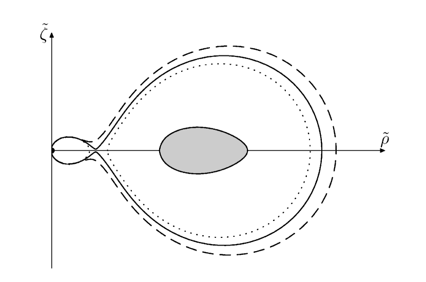
Figure 1: A coordinate representation of ergosurfaces for three configurations consisting of a black hole (coordinate origin) surrounded by a fluid ring (shaded area). The values of the parameters, in the notation of [2], are $\varrho_{\mathrm{i}}/\varrho_{\mathrm{o}}=0.55$, $r_{\mathrm{c}}/\varrho_{\mathrm{o}}=0.015$, $J_{\mathrm{c}}/\varrho_{\mathrm{o}}^{2}=0.05$, with $V_{0}=-1.45$ (dashed line), $V_{0}=-1.396$ (solid line) and $V_{0}=-1.35$ (dotted line). The shape of the ring (here corresponding to the ergosurface indicated by a solid line) is represented by the shaded area and differs only minimally between the three configurations. The coordinates $\tilde{\varrho}$ and $\tilde{\zeta}$ are related to $\varrho$ and $\zeta$ by a conformal transformation.

A purely vacuum example of this kind is hinted at in [18, Fig. 2]. Finally, Figures 2-4 show a purely vacuum example within the Kramer-Neugebauer family of solutions [9], where the parameters which are being varied are the $\beta_{i}$’s of [20].

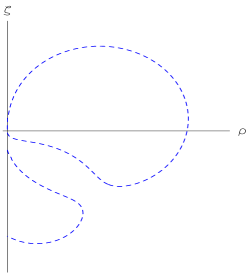
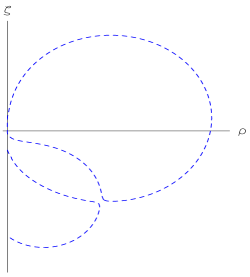
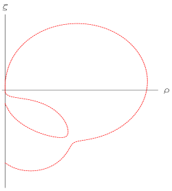
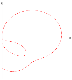
Figure 2: Coalescing ergosurfaces in the “double-Kerr” family of metrics in the $(\varrho,\zeta)$ half-plane, with one black hole extreme. We use a parameterization as in [20]. In all five cases the event horizon of the degenerate black hole lies at the origin, thus $\alpha_{1}=0$, while $\alpha_{2}=-1/6$, $\alpha_{3}=-1$, and with the $\beta_{a}$’s, $a=1,2$ of the form $\beta_{a}=-b_{a}(1+\mathrm{i})$, where: 1) $b_{1}=0.6$, $b_{2}=1.5$; 2) $b_{1}=0.62$, $b_{2}=1.66$; 3) $b_{1}=0.6218704381$, $b_{2}=1.668809562$; 4) $b_{1}=0.62$, $b_{2}=1.68$; 5) $b_{1}=0.6$, $b_{2}=1.7$. Those solutions have both singular struts at the axis and singular rings away from the region where the coalescing of ergosurfaces occurs, but those singularities are irrelevant for the proof that there are no local obstructions to zeros of higher order.

While the value of the parameters found numerically, for which $f$ has a zero of order two, is only approximate, the existence of a nearby value with a second order zero follows from what has been said above together with the remaining results in this paper.

Similarly three ergosurfaces merging simultaneously will lead to a zero of order precisely three, and so on.

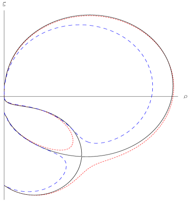
Figure 3: The first, third and fifth ergosurfaces of Figure 2 superimposed.

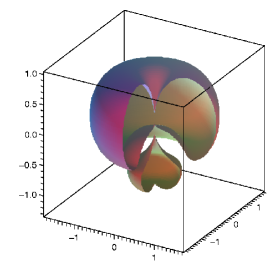
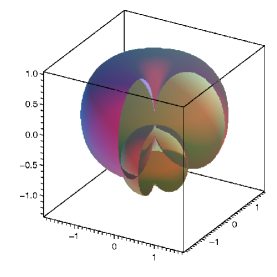
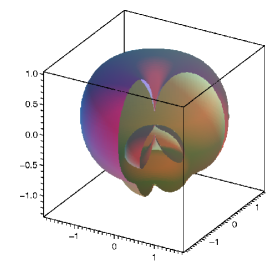
Figure 4: Coordinate representation in $\mathbb{R}^{3}$ of the first, third and fifth ergosurfaces from Figure 2. The cusps where the ergosurfaces meet the symmetry axis have a geometric character and also arise in the Kerr solution [19].

In order to study the zeros of higher order it is convenient to consider Taylor expansions of $f$ and $b$ to order $n\geq k$,

$$f(\rho,\zeta) = \sum_{0\leq i+j\leq n}\frac{\mathring{f}_{i,j}}{i!j!}(\rho-\rho_{0})^{i}(\zeta-\zeta_{0})^{j}+r_{n}\;,$$ (5.1)

where

$$\mathring{f}_{i,j}:=\frac{\partial^{i+j}f}{\partial^{i}\rho\partial^{j}\zeta}(\rho_{0},\zeta_{0})\;.$$

Similarly we denote the Taylor coefficients of $b$ by $\mathring{b}_{i,j}$.

Suppose that $f$ has a zero of order $k$ at $\vec{x}_{0}$. Note that the value $b(\rho_{0},\zeta_{0})=\Im{\mycal E}(\rho_{0},\zeta_{0})$ is irrelevant both for the equations and for the metric, so without loss of generality we may assume that ${\mycal E}(\rho_{0},\zeta_{0})=0$. ¿From now on we assume that this is the case. Let ${\mycal E}_{k}$ be the homogeneous polynomial in $\rho-\rho_{0}$ and $\zeta-\zeta_{0}$, of order $k$, obtained by keeping in the Taylor expansion only the terms of first non-vanishing order, similarly $f_{k}$. Thus, $f_{k}$ is a homogeneous polynomial in $\rho-\rho_{0}$ and $\zeta-\zeta_{0}$, of order $k$:

$$f_{k}(\rho,\zeta) = \sum_{i+j=k}\frac{\mathring{f}_{i,j}}{i!j!}(\rho-\rho_{0})^{i}(\zeta-\zeta_{0})^{j}\;.$$ (5.2)

The polynomial $f_{k}$ can be written in a convenient form, (5.4) below, as follows: suppose, for the moment, that $\rho-\rho_{0}$ is strictly positive, by homogeneity we can then write

$$f_{k}(\rho,\zeta)=(\rho-\rho_{0})^{k}P_{k}(w)\;,\qquad\mbox{where}\ w:=\frac{\zeta-\zeta_{0}}{\rho-\rho_{0}}\;,$$ (5.3)

for some non-trivial polynomial $P_{k}$ of order smaller than or equal to $k$. Let $\alpha_{i}\in{\mathbb{C}}$, $i=1,\ldots,n$, be distinct zeros of $P_{k}$, with multiplicities $m_{i}$, thus $P_{k}(w)=C\,\Pi_{i=1}^{n}(w-\alpha_{i})^{m_{i}}$, for some constant $C\in{\mathbb{C}}^{*}$. Hence

$$f_{k}(\rho,\zeta)=C(\rho-\rho_{0})^{m_{0}}\,\Pi_{i=1}^{n}\Big{(}\zeta-\zeta_{0}-\alpha_{i}(\rho-\rho_{0})\Big{)}^{m_{i}}\;,$$ (5.4)

where $m_{0}=k-m_{1}-\cdots m_{n}$. It should be clear that (5.4) remains true for all $\rho$, and not only for $\rho>\rho_{0}$ as assumed so far.

We will need the following:

Proposition 5.1.

Assume that $f$ and $b$ are smooth near $\vec{x}_{0}$. Then the function $b$, normalised so that $b(\vec{x}_{0})=0$, has a zero at $\vec{x}_{0}$ of precisely the same order as $f$.

Proof.

Let $k\in\mathbb{N}$ denote the order of the zero. For $k=1$ the result has already been established in Section 4, so we assume $k\geq 2$. We then have $f=O(|\vec{x}-\vec{x}_{0}|^{k})$, $|Df|=O(|\vec{x}-\vec{x}_{0}|^{k-1})$, $\Delta f=O(|\vec{x}-\vec{x}_{0}|^{k-2})$, and (2.5) shows that

$$|Db|^{2}=O(|\vec{x}-\vec{x}_{0}|^{2k-2})\;.$$

Integrating radially around $\vec{x}_{0}$ gives $b=O(|\vec{x}-\vec{x}_{0}|^{k})$, hence the order of the zero of $b$ is larger than or equal to $k$.

To show the reverse inequality, suppose that $b=O(|\vec{x}-\vec{x}_{0}|^{k+1})$. Inserting the Taylor expansion of $f$ into (1.1) one finds that $f_{k}$ solves the equation

$$f_{k}\left(\frac{\partial^{2}f_{k}}{\partial\rho^{2}}+\frac{\partial^{2}f_{k}}{\partial\zeta^{2}}\right)=\left(\frac{\partial f_{k}}{\partial\rho}\right)^{2}+\left(\frac{\partial f_{k}}{\partial\zeta}\right)^{2}\;.$$ (5.5)

On the set $\Omega_{k}:=\{f_{k}>0\}$ define $u_{k}=\ln f_{k}$. Without loss of generality, changing $f$ to $-f$ if necessary, we can assume that $\Omega_{k}$ is non-empty, with $\vec{x}_{0}$ lying in the closure of $\Omega_{k}$. On $\Omega_{k}$, Equation (5.5) is simply the statement that $u_{k}$ is harmonic in the variables $(\rho,\zeta)$:

$$\Delta_{2}u_{k}:=\frac{\partial^{2}u_{k}}{\partial\rho^{2}}+\frac{\partial^{2}u_{k}}{\partial\zeta^{2}}=0\;.$$ (5.6)

¿From (5.4) we have, assuming $C\neq 0$,

$$u_{k}=\ln C+m_{0}\ln(\rho-\rho_{0})+\sum_{i=1}^{n}m_{i}\ln\Big{(}\zeta-\zeta_{0}-\alpha_{i}(\rho-\rho_{0})\Big{)}\;.$$

Inserting into (5.6) one obtains

$$\Delta_{2}u_{k} = -m_{0}\frac{1}{(\rho-\rho_{o})^{2}}-\sum_{i=1}^{n}m_{i}(1+\alpha_{i}^{2})\frac{1}{\Big{(}\zeta-\zeta_{0}-\alpha_{i}(\rho-\rho_{0})\Big{)}^{2}}=0\;.$$

Recalling that the $\alpha_{i}$’s are distinct, this is only possible if

$$m_{0}=0=m_{i}(1+\alpha_{i}^{2})\quad\forall\ i\;.$$

Reordering the $m_{i}$’s if necessary, as $u_{k}$ is real-valued we have proved that

$$u_{k}=\ln C+m_{1}\ln\Big{(}(\zeta-\zeta_{0})^{2}+(\rho-\rho_{0})^{2}\Big{)}\quad\Longleftrightarrow\quad f_{k}=C\Big{(}(\zeta-\zeta_{0})^{2}+(\rho-\rho_{0})^{2}\Big{)}^{m_{1}}\;.$$

Subsequently,

$$f=C\Big{(}(\zeta-\zeta_{0})^{2}+(\rho-\rho_{0})^{2}\Big{)}^{m_{1}}+O(|\vec{x}-\vec{x}_{o}|^{k+1})\;.$$ (5.7)

As the order of $\vec{x}_{0}$ is even, this proves Proposition 5.1 for all $k$ odd.

To continue, we note the following

Lemma 5.2.

Under the hypotheses of Proposition 5.1, let $\vec{x}_{0}$ be a zero of order two. Then the quadratic form defined by the Hessian $DDf(\vec{x}_{0})$ of $f$ has signature $(+-)$ or $(-+)$. This implies that second order zeros of $f$ are isolated.

Remark 5.3.

For further use we note that the derivation of (5.8)-(5.9) only uses the truncated equations (5.13)-(5.14) below. Furthermore, the calculations here — and therefore their conclusions — remain valid when a supplementary error term $o(|\vec{x}-\vec{x}_{0}|^{3})$ is allowed at the right-hand-side of (2.5).

Proof.

The result is obtained by a calculation, the simplest way proceeds as in the proof of Theorem 5.6 below. Alternatively, one can use Maple or Mathematica, the interested reader can download the worksheets from http://th.if.uj.edu.pl/~szybka/CMS; that last calculation has been done as follows: Consider the polynomials $W_{a}$, $a=1,2$, obtained by inserting the Taylor expansion of $f$ and $b$, with $\mathring{f}=D\mathring{f}=0$, into equations obtained by multiplying (2.5) and (2.6) with $\rho$. The requirement that those polynomials vanish up-to-and-including order two imposes the following alternative sets of conditions:

I. $$\mathring{b}_{2,0}=\mathring{b}_{1,1}=\mathring{b}_{0,2}=\mathring{f}_{1,1}=0\;,\quad\mathring{f}_{2,0}=\mathring{f}_{0,2}\in\mathbb{R}\;,$$ (5.8)

II. $$\mathring{f}_{2,0}=-\mathring{f}_{0,2}=-\mathring{b}_{1,1}\in\mathbb{R}\;,\quad\mathring{b}_{0,2}=-\mathring{f}_{1,1}=-\mathring{b}_{2,0}\in\mathbb{R}\;,$$ (5.9)

as well as a set which is related to II. above by exchanging $b$ with $-b$. The first set leads to $\mathring{f}_{0,2}=0$ when requiring that the polynomials $W_{a}$ just defined vanish to one order higher, so that the first set cannot occur for zeros of second order. One then checks that the set II. leads to Lorentzian signature of $DDf$, unless vanishing.

Clearly the Hessian of $f$ given by (5.7) does not have indefinite signature when $m_{1}=1$, proving Proposition 5.1 for zeros of order two.

It remains to consider $m_{1}\in\mathbb{N}$ satisfying $m_{1}\geq 2$. Replacing $f$ by $-f$ if necessary, it follows from (5.7) that $f$ is strictly positive in a neighborhood of $\vec{x}_{0}$, so that we can define

$$g:=f^{1/m_{1}}\;.$$

Usual arguments (cf., e.g., [11]), show that $g$ is smooth and has a zero of order two at $\vec{x}_{0}$. From (2.5) one has

$$\displaystyle g\Delta g-|Dg|^{2}=\frac{1}{m_{1}}g^{2}\underbrace{\frac{|Db|^{2}}{f^{2}}}_{O(1)}=O(|\vec{x}-\vec{x}_{0}|^{4})\;.$$ (5.10)

Taylor expanding $g$ up to order $o(|\vec{x}-\vec{x}_{0}|^{4})$ and inserting into (5.10) gives $C=0$ (see Remark 5.3), proving Proposition 5.1.

5.1 Simple zeros

A zero of $f$ of order $k$ will be said to be simple if all the $\alpha_{i}$’s in (5.4) are real and have multiplicities one, with $m_{0}\in\{0,1\}$. We will show below that zeros of finite order of solutions of Ernst equations are simple. Somewhat to our surprise, for such zeros Theorem 4.1 generalises as follows:

Theorem 5.4.

The conclusions of Theorem 1.1 are valid under the supplementary condition that $f$ has only simple zeros at the ${\mycal E}$–ergosurface $E_{f}:=\{f=0,\rho>0\}$.

Proof.

As pointed out by Malgrange [11, end of Section 3], simplicity implies that near $\vec{x}_{0}$ there exist smooth functions $\phi_{a}$, $a=1,\ldots,k$, with $\phi_{a}(\vec{x}_{0})=0$ and with nowhere-vanishing gradient, together with a strictly positive smooth function $g$ such that we can write

$$f=\phi_{1}\cdots\phi_{k}g\;.$$ (5.11)

(Supposing that $m_{0}=0$, the $\phi_{a}$’s have the Taylor expansion $\phi_{a}=\zeta-\zeta_{0}-\alpha_{a}(\rho-\rho_{0})+O(|\vec{x}-\vec{x}_{0}|^{2})$; if $m_{0}=1$, then one has $\phi_{1}=\rho-\rho_{0}+O(|\vec{x}-\vec{x}_{0}|^{2})$, with the remaining Taylor expansions of the same form as before. For $k=2$ this is a special case of Morse’s theorem [6, Theorem 6.9, p. 65].)

Equation (5.11) shows that $E_{f}$ is, near $\vec{x}_{0}$, the union of the smooth submanifolds $\{\phi_{a}=0\}$. On each of those $Df$ is non-vanishing, except at the origin. Passing to a small neighborhood of $\vec{x}_{0}$ if necessary, we can assume that each of the sets $\{\phi_{a}=0,Df\neq 0\}$ has precisely two components.

Consider a connected component of $\{\phi_{1}=0\}$, by Section 4 Equation (4.1) holds there. Suppose that the lower sign arises on this component, then the same lower sign has to arise on the remaining component of $\{\phi_{1}=0\}$, because the inversion $\vec{x}-\vec{x}_{0}\to-\vec{x}+\vec{x}_{0}$ maps each component to the accompanying one up to quadratic terms, and because $Db$ has, in the leading order of its Taylor development, the same parity as $Df$ by Proposition 5.1.

We consider the function $\sigma_{\rho}$ as in (4.5), an identical argument applies to $\sigma_{\zeta}$ and to $\kappa_{\rho}$, $\kappa_{\zeta}$. Using a coordinate system $(y^{1},y^{2})$ with $\phi_{1}=y^{1}$ we have a Taylor expansion

$$\sigma_{\rho}(y^{1},y^{2})=\sigma_{\rho,0}(y^{2})+\sigma_{\rho,1}(y^{2})y^{1}+\sigma_{\rho,2}(y^{1},y^{2})(y^{1})^{2}\;.$$ (5.12)

Note that $f$ has a simple zero away from the origin on the axis $\{y^{1}=0\}$, so by the results in Section 4 the functions $\sigma_{\rho,0}$ and $\sigma_{\rho,1}$ vanish there. By continuity they also vanish at the origin, thus $\sigma_{\rho}$ factorises as

$$\sigma_{\rho}=\sigma^{\prime}_{\rho}\phi_{1}^{2}$$

for a smooth function $\sigma^{\prime}_{\rho}:=\sigma_{\rho,2}$.

We introduce a new coordinate system $(z^{1},z^{2})$ in which $z^{1}=\phi_{2}$. We Taylor expand $\sigma^{\prime}_{\rho}$ as in (5.12), with the $y^{i}$’s there replaced by $z^{i}$’s, etc. The equations

$$0 = \sigma_{\rho}|_{z^{1}=0,z^{2}\neq 0}=\sigma^{\prime}_{\rho}|_{z^{1}=0,z^{2}\neq 0}\underbrace{\phi_{1}^{2}|_{z^{1}=0,z^{2}\neq 0}}_{\neq 0}\;,$$

$$0 = d\sigma_{\rho}|_{z^{1}=0,z^{2}\neq 0}=d\sigma^{\prime}_{\rho}|_{z^{1}=0,z^{2}\neq 0}\underbrace{\phi_{1}^{2}|_{z^{1}=0,z^{2}\neq 0}}_{\neq 0}$$

$$+2\underbrace{\sigma^{\prime}_{\rho}|_{z^{1}=0,z^{2}\neq 0}}_{=0}(\phi_{1}d\phi_{1})|_{z^{1}=0,z^{2}\neq 0}\;,$$

show that the function $\sigma^{\prime}_{\rho}$ vanishes, together with its first derivatives, away from the origin on the axis $\{z^{1}=0\}$. We conclude as before that $\sigma^{\prime}_{\rho}$ factorises as $\sigma^{\prime}_{\rho}=\sigma^{\prime\prime}_{\rho}\phi_{2}^{2}$ for a smooth function $\sigma^{\prime\prime}_{\rho}$, hence $\sigma_{\rho}$ factorises as

$$\sigma_{\rho}=\sigma^{\prime\prime}_{\rho}\phi_{1}^{2}\phi_{2}^{2}\;.$$

Continuing in this way, in a finite number of steps one obtains

$$\sigma_{\rho}=\hat{\sigma}_{\rho}\phi_{1}^{2}\cdots\phi_{k}^{2}\;,$$

and the result easily follows.

5.2 Zeros of finite order are simple

Consider a zero of $f$ of order $k<\infty$, with $\rho_{0}>0$, then the leading order Taylor polynomials $f_{k}$ and $b_{k}$ solve the truncated equations

$$f_{k}\left(\frac{\partial^{2}f_{k}}{\partial\rho^{2}}+\frac{\partial^{2}f_{k}}{\partial\zeta^{2}}\right)=\left(\frac{\partial f_{k}}{\partial\rho}\right)^{2}+\left(\frac{\partial f_{k}}{\partial\zeta}\right)^{2}-\left(\frac{\partial b_{k}}{\partial\rho}\right)^{2}-\left(\frac{\partial b_{k}}{\partial\zeta}\right)^{2}\;,$$ (5.13)

$$f_{k}\left(\frac{\partial^{2}b_{k}}{\partial\rho^{2}}+\frac{\partial^{2}b_{k}}{\partial\zeta^{2}}\right)=2\Big{(}\frac{\partial f_{k}}{\partial\rho}\frac{\partial b_{k}}{\partial\rho}+\frac{\partial f_{k}}{\partial\zeta}\frac{\partial b_{k}}{\partial\zeta}\Big{)}\;.$$ (5.14)

Let

$$f_{k}+\mathrm{i}b_{k}\equiv{\mycal E}_{k}=\alpha(z-z_{0})^{k}\;,$$ (5.15)

where $\alpha\in{\mathbb{C}}$, with $z=\rho+\mathrm{i}\zeta$. It is straightforward, using the Cauchy-Riemann equations, to check that functions of this form satisfy (5.13)-(5.14), for all $k\in\mathbb{N}$. (In fact, both the left- and right-hand-sides then vanish identically.) Those solutions have been found by inspection of the solutions found by Maple for $k=2$ and by Singular [8, 7] for $k=3$ and $4$. In fact, both the Singular–generated solutions, as well as our remaining computer experiments using Singular, played a decisive role in our solution of the problem at hand.

Let us show that:

Lemma 5.5.

Zeros of $f_{k}$ given by (5.15) are simple.

Proof.

Indeed, the equation $f_{k}=0$ is equivalent to

$$\alpha(z-z_{0})^{k}=\mathrm{i}\beta\;,$$

for some $\beta\in\mathbb{R}$. This is easily solved; we write $\alpha=|\alpha|e^{\mathrm{i}\theta}$, and set

$$\alpha_{\ell}=\tan\Big{(}\frac{{(2\ell+1)\pi}-2\theta}{2k}\Big{)}\;,\quad\ell=1,\ldots,k\;.$$

Assuming $\alpha_{\ell}\neq\pm\infty$ for all $\ell$, we obtain $k$ distinct real lines $z_{0}+\mathbb{R}(1+\mathrm{i}\alpha_{\ell})$ on which $\Re{\mycal E}_{k}$ vanishes, and simplicity follows. The remaining cases are analysed similarly, and are left to the reader.

Another non-trivial, “polarised”, family of solutions of (5.13)-(5.14) is provided by $b_{k}=0$, $f_{k}=C\Big{(}(\rho-\rho_{0})^{2}+(\zeta-\zeta_{0})^{2}\Big{)}{}^{m}$, $m\in\mathbb{N}$. As mentioned in Section 3, there exist associated static solutions of the Ernst equations. However, as already pointed out (compare Remark 5.3), neither those, nor any other solutions with this $f_{k},b_{k}$, are smooth across $E_{f}$.

Setting $z=\rho-\rho_{0}+\mathrm{i}(\zeta-\zeta_{0})$, the equations satisfied by ${\mycal E}_{k}=f_{k}+\mathrm{i}b_{k}$ take the form

$$({\mycal E}_{k}+\overline{{\mycal E}}_{k})\frac{\partial^{2}{\mycal E}_{k}}{\partial z\partial{\bar{z}}}=2\frac{\partial{\mycal E}_{k}}{\partial z}\frac{\partial{\mycal E}_{k}}{\partial{\bar{z}}}\;.$$ (5.16)

Since ${\mycal E}_{k}$ is a polyhomogeneous polynomial in $x$ and $y$, it can be written as

$${\mycal E}_{k}=\sum_{m=0}^{k}\beta_{m}z^{m}{\bar{z}}^{k-m}\;.$$

Inserting this into (5.16) we obtain

$$\sum_{1\leq m+j\leq 2k-1}m\beta_{m}\{(2j-k-m)\beta_{j}+(k-m)\bar{\beta}_{k-j}\}z^{m+j-1}{\bar{z}}^{2k-m-j-1}=0\;.$$

Hence, for $1\leq\ell\leq 2k-1$,

$$\sum_{m+j=\ell}\{(k-m)\bar{\beta}_{k-j}-(k+m-2j)\beta_{j}\}m\beta_{m}=0\;.$$ (5.17)

Since $\ell=0$ is trivial, we obtain $2k-2$ equations for $k+1$ numbers $\beta_{m}$, which should be rather restrictive, especially for $k\geq 3$. Nevertheless, as already pointed out, there exist non-trivial solutions. It is instructive to find them directly by inspection of (5.17). First, there is the obvious solution $\beta_{m}=0$ for $m\geq 1$, which corresponds to an anti-holomorphic ${\mycal E}_{k}=\beta_{0}{\bar{z}}^{k}$. Next, one checks that a collection with $\beta_{k}\neq 0$ but $\beta_{m}=0$ for $m<k$ provides a solution, which corresponds to a holomorphic ${\mycal E}_{k}=\beta_{k}z^{k}$. Finally, when $k=2n$, one checks that $\beta_{n}\in\mathbb{R}$, but $\beta_{m}=0$ for $m\neq k/2$, is a solution, which corresponds to a real ${\mycal E}_{2n}=\beta_{n}z^{n}{\bar{z}}^{n}=\beta_{n}(x^{2}+y^{2})^{n}$.

The computer algebra program Singular can be used to show that the above exhaust the list of solutions for $k$ less than or equal to eight. This turns out to be true for all $k<\infty$:

Theorem 5.6.

These are all solutions: thus the homogeneous polynomial ${\mycal E}_{k}$ is either holomorphic, or anti-holomorphic, or real and radial.

Proof.

The case $k=1$ is a straightforward calculation, so we assume $k>1$.

If ${\mycal E}_{k}$ is a solution, then so is its complex conjugate; this implies that if an ordered collection $\{\beta_{m}\}_{0\leq m\leq k}$ satisfies (5.17), then so does $\{\bar{\beta}_{k-m}\}_{0\leq m\leq k}$. Inserting this into (5.17) one obtains, again for $1\leq\ell\leq 2k-1$,

$$\sum_{m+j=\ell}\{(k-m){\beta}_{j}-(k+m-2j)\bar{\beta}_{k-j}\}m\bar{\beta}_{k-m}=0\;.$$ (5.18)

Consider (5.17) with $\ell=1$; since $1\leq m\leq\ell$ this enforces $m=1$, $j=0$, giving

$$\{(k-1)\bar{\beta}_{k}-(k+1)\beta_{0}\}\beta_{1}=0\;.$$ (5.19)

Similarly (5.18) with $\ell=1$ gives

$${\{(k-1){\beta}_{0}-(k+1)\bar{\beta}_{k}\}}\bar{\beta}_{k-1}=0\;.$$ (5.20)

Suppose, first, that $\beta_{0}\neq 0$. We will use induction arguments to establish the implication (5.21) below. So assume, for contradiction, that $\beta_{1}\neq 0$. Then $\bar{\beta}_{k}=(k+1)\beta_{0}/(k-1)\neq 0$ from (5.19), inserting into (5.20) we obtain $\beta_{k-1}=0$. But then (5.18) with $\ell=2$ gives

$$0=\{(k-2){\beta}_{0}-(k+2)\bar{\beta}_{k}\}\bar{\beta}_{k-2}=\underbrace{\frac{(k-2)(k-1)-(k+2)(k+1)}{k-1}\beta_{0}}_{\neq 0}\bar{\beta}_{k-2}\;,$$

hence $\beta_{k-2}=0$. Equation (5.18) with $\ell=3$ similarly gives now $\beta_{k-3}=0$. Continuing in this way one concludes in a finite number of steps that $\beta_{1}=0$, a contradiction. It follows that $\beta_{0}\neq 0$ enforces $\beta_{1}=0$.

Assume now, again for contradiction, that $\beta_{0}\neq 0$ and $\beta_{1}=0$ but $\beta_{2}\neq 0$. Equation (5.17) with $\ell=2$ gives

$$\{(k-2)\bar{\beta}_{k}-(k+2)\beta_{0}\}\beta_{2}=0\;.$$

If $k=2$ we obtain immediately a contradiction; otherwise $\bar{\beta}_{k}=(k+2)\beta_{0}/(k-2)\neq 0$, inserting into (5.20) we find $\beta_{k-1}=0$. But then (5.18) with $\ell=2$ gives

$$0=\{(k-2){\beta}_{0}-(k+2)\bar{\beta}_{k}\}\bar{\beta}_{k-2}=\underbrace{\frac{(k-2)^{2}-(k+2)^{2}}{k-1}\bar{\beta}_{k}}_{\neq 0}\bar{\beta}_{k-2}\;,$$

hence $\beta_{k-2}=0$. Continuing in this way one concludes in a finite number of steps that $\beta_{2}=0$, a contradiction. This shows that $\beta_{0}\neq 0$ and $\beta_{1}=0$ but $\beta_{2}\neq 0$ is incompatible with the equations.

It should be clear to the reader how to iterate this argument to obtain the implication

$$\beta_{0}\neq 0\ \mbox{ implies }\ \beta_{m}=0\ \mbox{ for }\ m=1,\ldots,k\;.$$ (5.21)

Using symmetry under complex conjugation, the hypothesis $\beta_{k}\neq 0$ leads to $\beta_{m}=0$ for $m=0,\ldots,k-1$.

It remains to analyse what happens when $\beta_{0}=\beta_{k}=0$, which we assume from now on. Suppose (for contradiction if $k>2$) that $\beta_{1}\neq 0$. Recalling that $k>1$, (5.17)-(5.18) with $\ell=2$ give

$$(\bar{\beta}_{k-1}-\beta_{1})\beta_{1}=0=({\beta}_{1}-\bar{\beta}_{k-1})\bar{\beta}_{k-1}\;.$$

If $k=2$ we obtain $\beta_{1}\in\mathbb{R}$, and we are done.

Otherwise $\beta_{k-1}=\bar{\beta}_{1}\neq 0$ and (5.18) with $\ell=3$ gives

$$\{(k-1)\beta_{2}-(k+1)\bar{\beta}_{k-2}\}\beta_{1}=0\;.$$

When $k=3$ this gives a contradiction, and the result is established for this value of $k$.

For $k\geq 4$ the proof will be finished by more induction arguments, as follows: Suppose, to start with, that $\beta_{k}=0$ and that there exist $k_{0},k_{1}\in\mathbb{N}$, $1\leq k_{1}\leq k_{0}\leq k/2$, such that $\beta_{m}=0$ for $0\leq m\leq k_{0}-1$ and for $k-k_{1}<m\leq k$ but $\beta_{k_{0}}\neq 0$. (The case $k_{1}>k_{0}$ can be reduced to this one by replacing ${\mycal E}_{k}$ with its complex conjugate.) With these hypotheses (5.17) can be rewritten as

$$\sum_{k_{0}\leq m\leq\min(k-k_{1},\ell-k_{1})}\{(k-m)\bar{\beta}_{k-(\ell-m)}-(k+3m-2\ell)\beta_{\ell-m}\}m\beta_{m}=0\;.$$ (5.22)

Equation (5.22) with $\ell=k_{0}+k_{1}\leq k$ gives:

$$(k-k_{0})\bar{\beta}_{k-k_{1}}=(k+k_{0}-2k_{1})\beta_{k_{1}}$$

which equals zero unless $k_{1}=k_{0}$. It follows that we can without loss of generality assume that $k_{1}=k_{0}$ and

$${\beta}_{k-k_{0}}=\bar{\beta}_{k_{0}}\;.$$

We can now rewrite (5.18) as

$$\sum_{k_{0}\leq m\leq\min(k-k_{0},\ell-k_{0})}\{(k-m){\beta}_{\ell-m}-(k+3m-2\ell)\bar{\beta}_{k-(\ell-m)}\}m\bar{\beta}_{k-m}=0\;.$$ (5.23)

Suppose that $k=2k_{0}$; then (5.23) leads immediately to the restriction $\beta_{k_{0}}\in\mathbb{R}$, giving a real radial solution, as desired. Otherwise, choosing $\ell=2k_{0}+1$ in (5.23) one obtains

$$(k-k_{0})k_{0}\beta_{k_{0}+1}=[(k-k_{0})k_{0}+2]\bar{\beta}_{k-k_{0}-1}\;.$$

Equation (5.22) with $\ell=2k_{0}+1$ gives

$$(k-k_{0})k_{0}\bar{\beta}_{k-k_{0}-1}=[(k-k_{0})k_{0}+2]\beta_{k_{0}+1}\;.$$

It follows that

$$\beta_{k_{0}+1}=\beta_{k-k_{0}-1}=0\;.$$

Our aim now is to show (5.24) below, by a last induction. So, suppose there exists $k_{2}\in\mathbb{N}$ satisfying $k_{0}<k_{2}<k-k_{0}$ such that $\beta_{m}=0$ for $k_{0}<m<k_{2}$ and for $k-k_{2}<m<k-k_{0}$; we have shown that this is true with $k_{2}=k_{0}+2$. Equation (5.23) with $\ell=k_{0}+k_{2}$ gives

$$(k-k_{0})k_{0}\beta_{k_{2}}=[(k-k_{0})k_{0}+2(k_{2}-k_{0})^{2}]\bar{\beta}_{k-k_{2}}\;.$$

But from (5.22) again with $\ell=k_{0}+k_{2}$ one obtains

$$(k-k_{0})k_{0}\bar{\beta}_{k-k_{2}}=[(k-k_{0})k_{0}+2(k_{2}-k_{0})^{2}]\beta_{k_{2}}\;.$$

This allows us to conclude that

$$\beta_{m}=0\ \mbox{ except if }\ m=k_{0}\ \mbox{ or if }\ m=k-k_{0}\;,\ \mbox{ with }\ \beta_{k-k_{0}}=\bar{\beta}_{k_{0}}\;.$$ (5.24)

Equation (5.23) with $\ell=k$ gives now $\beta_{k_{0}}=0$ (recall that we have assumed $k\neq 2k_{0}$), a contradiction, and the theorem is proved.

We can now pass to the

Proof of Theorem 1.1: Theorem 5.6 gives the list of all possible ${\mycal E}_{k}$’s. The real ones do not lead to smooth $f$’s by Proposition 5.1. The holomorphic ones lead to simple zeros by Lemma 5.5; the same is true for the anti-holomorphic ones, because the condition of simplicity is preserved by complex-conjugation of ${\mycal E}$. The result follows now from Theorem 5.4.

Acknowledgements We wish to thank G. Alekseev, M. Ansorg, R. Beig, M.-F. Bidaut-Véron, M. Brickenstein, S. Janeczko, J. Kijowski, G. Neugebauer, D. Petroff and L. Véron for useful comments or discussions. We acknowledge hospitality and financial support from the Newton Institute, Cambridge (PTC, RM, SSz), as well as the AEI, Golm (PTC) during work on this paper.

References

- [1] M. Ansorg, Differentially rotating disks of dust: Arbitrary rotation law, Gen. Rel. Grav. 33 (2001), 309–338, gr-qc/0006045.
- [2] M. Ansorg and D. Petroff, Black holes surrounded by uniformly rotating rings, Phys. Rev. D72 (2005), 024019, gr-qc/0505060.
- [3] B. Carter, Black hole equilibrium states, Black Holes (C. de Witt and B. de Witt, eds.), Gordon & Breach, New York, London, Paris, 1973, Proceedings of the Les Houches Summer School.
- [4] P.T. Chruściel, R. Meinel, and S. Szybka, The Ernst equation and ergosurfaces, (2005), Newton Institute Preprint NI05081-GMR, http://www.newton.cam.ac.uk/preprints/NI05081.pdf.
- [5] F.J. Ernst, New formulation of the axially symmetric gravitational field problem, Phys. Rev. 167 (1968), 1175–1178.
- [6] M. Golubitsky and V. Guillemin, Stable mappings and their singularities, Graduate Texts in Mathematics 14, New York - Heidelberg - Berlin: Springer-Verlag, 1973.
- [7] G.-M. Greuel and G. Pfister, A Singular introduction to commutative algebra, with contributions by O. Bachmann, C. Lossen and H. Schönemann, Springer-Verlag, Berlin, 2002. MR MR1930604 (2003k:13001)
- [8] G.-M. Greuel, G. Pfister, and H. Schönemann, Singular, a computer algebra system for polynomial computations, URL http://www.singular.uni-kl.de.
- [9] D. Kramer and G. Neugebauer, The superposition of two Kerr solutions, Phys. Lett. A 75 (1979/80), 259–261. MR MR594394 (81m:83014)
- [10] J. Lewandowski and T. Pawłowski, Extremal isolated horizons: A local uniqueness theorem, Class. Quantum Grav. 20 (2003), 587–606, gr-qc/0208032.
- [11] B. Malgrange, Idéaux de fonctions différentiables et division des distributions, Distributions, Ed. Éc. Polytech., Palaiseau, 2003, http://www.math.polytechnique.fr/xups/vol03.html, pp. 1–21. MR MR2065138
- [12] V.S. Manko and E. Ruiz, Extended multi-soliton solutions of the Einstein field equations, Class. Quantum Grav. 15 (1998), 2007–2016. MR MR1633190 (99m:83045)
- [13] H. Müller zum Hagen, On the analyticity of stationary vacuum solutions of Einstein’s equation, Proc. Cambridge Philos. Soc. 68 (1970), 199–201. MR 41 #5017
- [14] G. Neugebauer, A general integral of the axially symmetric stationary Einstein equations, Jour. Phys. A 13 (1980), L19–L21. MR MR558632 (80k:83024)
- [15] G. Neugebauer, A. Kleinwächter, and R. Meinel, Relativistically rotating dust, Helv. Phys. Acta 77 (1996), 472–489.
- [16] G. Neugebauer and R. Meinel, General relativistic gravitational field of a rigidly rotating disk of dust: Solution in terms of ultraelliptic functions, Phys. Rev. Lett. 75 (1995), 3046.
- [17] G. Neugebauer and R. Meinel, Progress in relativistic gravitational theory using the inverse scattering method, Jour. Math. Phys. 44 (2003), 3407–3429, gr-qc/0304086.
- [18] K. Oohara and H. Sato, Structure of superposed two Kerr metrics, Progr. Theoret. Phys. 65 (1981), 1891–1900. MR MR626966 (82m:83009)
- [19] N. Pelavas, N. Neary, and K. Lake, Properties of the instantaneous ergo surface of a Kerr black hole, Class. Quantum Grav. 18 (2001), 1319–1332, gr-qc/0012052.
- [20] J. A. Rueda, V. S. Manko, E. Ruiz, and J. D. Sanabria-Gomez, The double-Kerr equilibrium configurations involving one extreme object, Class. Quantum Grav. 22 (2005), 4887–4894, gr-qc/0508101.
- [21] G. Weinstein, On rotating black–holes in equilibrium in general relativity, Commun. Pure Appl. Math. XLIII (1990), 903–948.
- [22] M. Yamazaki, Stationary line of Kerr masses kept apart by gravitational spin-spin interaction, Phys. Rev. Lett. 50 (1983), 1027–1030. MR MR700070 (84e:83021)