Excising das All: Evolving Maxwell waves beyond scri

Abstract

We study the numerical propagation of waves through future null infinity in a conformally compactified spacetime. We introduce an artificial cosmological constant, which allows us some control over the causal structure near null infinity. We exploit this freedom to ensure that all light cones are tilted outward in a region near null infinity, which allows us to impose excision-style boundary conditions in our finite difference code. In this preliminary study we consider electromagnetic waves propagating in a static, conformally compactified spacetime.

I Introduction

The motivation for the present work is the matching of a computational model of a source of gravitational waves (such as a compact object binary) to the cosmological environment through which any emitted signal travels to a detector. The transmission phase is well understood and is essentially the propagation of a linearized gravitational wave through a background cosmology which includes such effects as a cosmological redshift and gravitational lensing due to intervening masses, plus the kinetic effects of the detector’s motions. For these purposes the geometrical optics approximation is often adequate. Although implementing this transmission model in observatory data analysis demands skill, it is simpler than the electromagnetic case where interactions with dust, gas and plasmas en route must also be considered. In this large scale background the source can be taken to be a point source of linearized gravitational waves having some specific antenna patterns and wave forms. The more unsettled question then is how to extract from a detailed model of a wave generation system the appropriate linearized wave. The most common assumption is that the wave generator can be modeled as existing in an asymptotically flat spacetime where waves propagating out to future null infinity (scri+ or $\mathscr{I}^{+}$) will be described there by linearized gravitation, originating from a point source in the cosmological context. This is clearly justified by the huge difference in scales between the size of the wave generator and the radius of curvature of its surrounding spacetime (the cosmos or a galaxy or stellar cluster). The question then is how to efficiently calculate and extract the waveforms at $\mathscr{I}^{+}$.

In the usual Cauchy evolutions on asymptotically flat spacelike hypersurfaces, the waves must be recognized at large distances from the source, possibly a long time after the source motions have ceased violent activity. One way to overcome this time lag is through the use of a retarded time coordinate. This works well in spherical symmetry Hernandez and Misner (1966); Baumgarte et al. (1995), but is poorly defined otherwise. The Pittsburgh group has used such characteristic evolution at larger distances while matching to more common Cauchy evolution in the interior Winicour (2005). The use of hyperboloidal time slices (some generalization of hyperboloids in Minkowski spacetime) appears attractive as a smooth transition from conventional time slices in central regions to asympotically null spacelike hypersurfaces toward infinity. Were such a slicing to be combined with a straightforward Cauchy evolution, the Courant time step condition would defeat the advantages of approximating retarded time, as the nearly infinite coordinate speed of light toward infinity would require infinitesimal time steps (since the Courant condition generally requires that $\Delta t/\Delta x<1/c$ for numerical stability). Thus hyperboloidal slicings effectively require a conformal compactification which makes the coordinate speed of light finite again Misner et al. (2003).

In addition to the use of hyperboloidal time slices and conformal compactification, we suggest two additional tools to ameliorate the extraction of outgoing waves in numerical evolutions. One is the use of artificial cosmology to convert the null hypersurface $\mathscr{I}^{+}$ into a spacelike hypersurface in the future of the initial Cauchy hypersurface as proposed in Misner (2006). This procedure fattens $\mathscr{I}^{+}$ into a shell of spacelike hypersurfaces by changing the value of the cosmological constant, plausible for the present universe, by many orders of magnitude so that the de Sitter horizon is located, not at cosmological distances, but merely well beyond the region where the wave generating mechanism can be influenced by it. In this sense it is similar to the computational tool of artificial viscosity which fattens a shock from its physical thickness on the order of the molecular mean free path into a much larger length which is still small in the range of scales that otherwise are met in the physical problem at hand. The second additional tool is the tilting of the null cones governing wave propagation in ways that ease the computational behavior in the unphysical (‘das All’) region beyond the de Sitter horizon and beyond $\mathscr{I}^{+}$.

The German noun “das All” refers to the Universe, but sometimes in a sense unfamiliar in English where it translates better as “outer space.” A spacecraft, after launch, might be described as entering das All. In the computations reported here, it is precisely this outer space — the physical details far from a source of gravitational (or in our case electromagnetic) waves — which is excised from the computational model in analogy to the way the internal mysteries/singularities of a black hole are often excised in computational models. We develop and implement the proposals made earlier in Refs. Misner et al. (2003); Misner (2006) and suggested above to obtain wave forms promptly at infinity by using hyperboloidal time slices in a Cauchy evolution, to avoid infinitesimal time steps through conformal compactification, to convert outer boundary conditions to excision boundary conditions by using an artificial cosmological constant, and to defend the physical domain against computational boundary errors by tilting the light cones further outward in the region beyond the outer horizon. The aim of this paper is to explore the application of this set of boundary treatment tools in a low cost application in order to see whether there are unexpected impediments to its application, and to get guidance for the best approaches for its application to larger problems.

The use of hyperboloidal slicings in numerical relativity has been carefully studied (e.g. Refs. Husa (2002); Friedrich (2002); Winicour (2005); Frauendiener (2004)), and there are existing numerical results generated on compactified domains (e.g. Ref. Pretorius (2005)). This paper contributes to this literature by combining these two techniques in a spacetime with an artificial cosmological structure designed to make it easier to construct boundary conditions at $\mathscr{I}^{+}$, and by studying the effectiveness of modifying the light cone structure in the region of the analytically continued spacetime exterior to $\mathscr{I}^{+}$ to prevent non-physical, incoming radiation from piling up on the non-physical side of $\mathscr{I}^{+}$. That said, our approach to the problem does not require special modifications to the form of the differential equations solved to model the physical problem. It should be compatible with existing numerical codes desgined to solve the initial problem, described by some variant of the the Einstein equations in an Arnowitt-Deser-Misner 3+1 decomposition Arnowitt et al. (1962).

Our work is also complementary to community wide efforts to use mesh refinement techniques in numerical relativity. Several groups have recently and successfully incorporated mesh refinement techniques into their Einstein solvers (i.e. Refs. Brügmann (1996); Choi et al. (2004); Imbiriba et al. (2004); Fiske et al. (2005); Schnetter et al. (2004); Sperhake et al. (2005); Pretorius (2005); Brügmann et al. (2004); Baker et al. (2006a, b)). This technology allows groups to push their computational boundaries to very large coordinate distances, reducing the effects of incoming radiation and constraint violating modes introduced by applying boundary conditions at a finite distance.

While mesh refinement has greatly increased the power of modern codes, it also has limitations. It is now fairly easy to surround a computational domain with coarser and coarser grids, but at some point the coarse grids cannot resolve a wavelength, see, e.g. Refs. Fiske et al. (2005) and (Fiske, 2004a, Section 4.3). They can, however, insulate the active, wave generation regions of the computational domain from boundary problems for a limited period of time. During this period waveforms have been successfully extracted from inner regions as small as 2.4 wavelengths from the center Baker et al. (2006b). The hyperboloidal slicings considered here and elsewhere have the advantage that they asymptote to the outgoing light cones in the spacetime. Outgoing waves, therefore, appear asymptotically constant and require very few points to resolve them all the way to $\mathscr{I}^{+}$.

The rest of the paper is organized as follows: In Sec. II, we briefly summarize the formalism we use in our code, both for the background spacetime metric and for the Maxwell equations themselves. In Sec. III we describe the numerical methods used to solve the equations. We summarize the numerical results and discuss the implications for future work in Sec. IV. Additional detail is provided in the Appendix.

II Formalism

II.1 Spacetime Metric

As in Ref. Misner (2006) the background metric for this study will be the de Sitter spacetime

$$ds^{2}=-dT^{2}+dX^{2}+dY^{2}+dZ^{2}+(R^{2}/L^{2})(dT-dR)^{2}$$ (1)

with an artificial cosmological constant $\Lambda=+3/L^{2}$. We are interested in the limit $1/L^{2}\rightarrow 0$ when this becomes Minkowski spacetime, and the cosmological constant is used to make boundary conditions numerically simpler (we hope) at the de Sitter horizon than they would be at flat spacetime’s $\mathscr{I}^{+}$. The de Sitter horizon is the null hypersurface $R=L$ in this metric. We introduce the coordinate changes

$$\frac{T}{s} = u+\frac{r^{2}/2}{1-r^{2}/4}$$ (2a)

$$\frac{X^{i}}{s} = \frac{x^{i}}{1-r^{2}/4}$$ (2b)

as used in Refs. Misner et al. (2003); Misner (2006), where $R^{2}=X^{2}+Y^{2}+Z^{2}\equiv X^{i}X^{i}$, $r^{2}=x^{2}+y^{2}+z^{2}\equiv x^{i}x^{i}$, and $s$ is a constant scaling factor whose geometrical significance can be read from Eq. (3) below. This brings $\mathscr{I}^{+}$ in to $r=2$ in the Minkowski case and in the de Sitter case makes this a spacelike hypersurface beyond the de Sitter horizon which is part of de Sitter spacetime’s future causal boundary which is also called $\mathscr{I}^{+}$. The hypersurfaces of constant $u$ are then hyperboloids

$$[T-s(u-1)]^{2}-R^{2}=s^{2}$$ (3)

in Minkowski spacetime and are also asymptotically null spacelike hypersurfaces in the de Sitter modification. These hyperboloids in Minkowski spacetime have constant curvature of radius $s$ which is therefore the scale of the region in which they are approximately flat. Also the time interval $\Delta T$ at the spatial origin between the $u$ slice on which a light signal is emitted there and the $u$ slice on which it reaches $\mathscr{I}+$ is $\Delta u=1$ or $\Delta T=s$. Thus $s$ may also be called the scri-delay. This coordinate change leads to a metric which is singular at $r=2$, but only in a conformal factor $s^{2}/q^{2}=s^{2}/(1-r^{2}/4)^{2}$ which does not appear in the Maxwell equations. Thus we can drop this conformal factor and our test problem is to solve the Maxwell equations in the resultant metric which is of the form

$$ds^{2}=-\alpha^{2}dt^{2}+\gamma_{ij}(dx^{i}+\beta^{i}dt)(dx^{j}+\beta^{j}dt)$$ (4)

with $t=u$. For use in later modifications we include a function $W(r)$ in the definition of the metric functions in (4). For now we choose $W=0$ and then the following equations give the analytically continued and conformally regulated de Sitter metric described above:

$$\alpha = \frac{(1-W)(1+\frac{r^{2}}{4})}{\sqrt{1+\left(\frac{sS}{L}\right)^{2}}}$$ (5a)

$$\beta^{i} = -x^{i}\frac{1-W+\left(\frac{s}{L}\right)^{2}S}{1+\left(\frac{sS}{L}\right)^{2}}$$ (5b)

$$\gamma_{ij} = \left(\frac{sS}{Lr}\right)^{2}x_{i}x_{j}+\delta_{ij}$$ (5c)

where

$$S=\frac{(1-W)r}{(1+\frac{r}{2})^{2}}+\frac{1}{4}\left(\frac{L}{s}\right)^{2}W.$$ (6)

To see the behavior of the light cones for this regulated metric, we calculate the coordinate speed of light $dr/du$ in radial null directions. This gives

$$v=\frac{r+r(s^{2}/L^{2})S\pm(1+\frac{r^{2}}{4})}{1+(s^{2}/L^{2})S^{2}}\quad.$$ (7)

For the de Sitter values above this reduces to

$$v_{\rm out}=(1+\tfrac{1}{2}r)^{2}$$ (8)

and

$$v_{\rm in}=\frac{-(1-\tfrac{1}{2}r)^{2}+(s^{2}/L^{2})(1+\tfrac{1}{2}r)^{2}S^{2}}{1+(s^{2}/L^{2})S^{2}}\quad.$$ (9)

Note that the constant $r$ hypersurfaces are never spacelike when $s/L=0$ since then the inward speed of light is $v_{\rm in}\leq 0$. When the de Sitter option is used one finds $v_{\rm in}>0$, i.e., both the inward and the outward sides of the lightcone point toward increasing $r$, for an interval around $r=2$.

In evolution codes which permit setting the computational boundary on a coordinate sphere (such as those described in Kidder et al. (2005); Thornburg (2004); Lehner et al. (2005); Diener et al. (2005)) the outer boundary could be set at $r=2$ or slightly beyond in the metric described above (or ones asymptotically similar). However, if a cubic boundary enclosing $\mathscr{I}^{+}$ is to be used, there are additional behaviors beyond $\mathscr{I}^{+}$ that need attention. For example, if the artificial de Sitter horizon is set at $L=10s$, then the $r=\text{constant}$ hypersurfaces are spacelike only in the narrow interval of (approximately) $r=1.81$ to $r=2.21$. But a boundary cube enclosing $r=2$ has corners at $r=2\sqrt{3}\approx 3.46$. Thus on most of such a cubic boundary the light cones (from Eq. (9)) would allow inwardly propagating waves, requiring careful attention to the boundary conditions which one hopes to avoid.

Fig. 1 below shows the coordinate speeds for light rays on the inward side of the light cone $v_{\text{in}}$, on the outward side of the light cone $v_{\text{out}}$, and for a timelike center of the light cone $v_{\text{center}}=-\beta$ normal to the time slices of constant $u$.

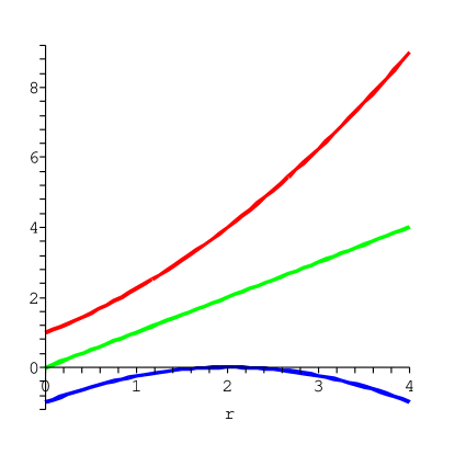
Figure 1: Coordinate speeds for the de Sitter lightcone: inward ($v_{\text{in}}$, blue, lowest curve), normal to the spacelike time slices ($-\beta$, green, middle curve), and outward ($v_{\text{out}}$, red, highest curve). For the Minkowski metric the graph looks very similar, except that $v_{\text{in}}$ is there never positive.

This allows light rays to move inward ($v_{\text{in}}<0$) in some of the region beyond $\mathscr{I}^{+}$ within a cubical computational grid.

In this case we suggest that the metric be modified outside $r=2$ so that all $r=\text{constant}$ hypersurfaces beyond $r=2$ are spacelike — i.e., so that $v_{\rm in}>0$ in the entire computational domain beyond $r=2$. Analytically this would have no effect on the physical solution inside $r=2$ provided all fields propagate causally. This modification is also straightforward to do in the test case of a Maxwell field with a fixed background metric. If these methods were to be developed for the Einstein equations (without using a spherical boundary such as $r=2$) it would necessitate distinguishing, in the Einstein equations beyond $r=2$, the $g_{\mu\nu}$ metric being evolved from the appearances of the metric as coefficients of the principle derivatives which determine the causal relations in the evolution algorithm.

In the Minkowski case $s/L=0$ (no artificial cosmology) it is not possible to make a $C^{2}$ change in the metric only beyond $r=2$ which avoids inward pointing null rays just beyond $r=2$ — in that case one has, from the $r\leq 2$ formula above for $v_{\rm in}$ that $(d^{2}/dr^{2})v_{\rm in}=-\tfrac{1}{2}$ at $r=2$ so that $v_{\rm in}$ must have a local maximum value of zero at that point and is necessarily negative (inward) in a neighborhood of that point, including some $r>2$ points. For the de Sitter case there is again a maximum of $v_{\rm in}$ near $r=2$, but its value there is positive so it can be smoothly turned upward (to avoid zero or negative values) in suitable intervals beyond the de Sitter horizon (and beyond $r=2$ for small values of $s/L$).

In Eqs. (5) and (6), assuming $s/L>0$, we choose to take

$$W(r)=\Theta(r-2)\frac{(r-2)^{4}}{\left[\left(r-2\right)^{2}+\frac{1}{2}\right]^{2}}$$ (10)

to be a smooth step function that modifies the metric beyond $r=2$ in a way that keeps the “incoming” coordinate speed of light $v_{in}=dr/du$ positive (that is outgoing) when $r>2$. The function $W$ is a $C^{3}$ modification of $\Theta(r-2)$, the Heaviside step function that jumps from 0 to 1 at $r=2$. Fig. 2 below shows the modified light cone directions in this case.

Note that for $r\leq 2$, where $W=0$, this metric has the surprising property that the outgoing speed of light $v_{out}=(1+r/2)^{2}$ is independent of the cosmological constant parameter $L$. Although in general the presence of a cosmological constant alters the causal structure of a spacetime, and indeed it does modify the ingoing radial speed of light in the present example, it does not change the outgoing radial speed of light from that of the original Minkowski spacetime. This fact will prove useful for numerical diagnostics.

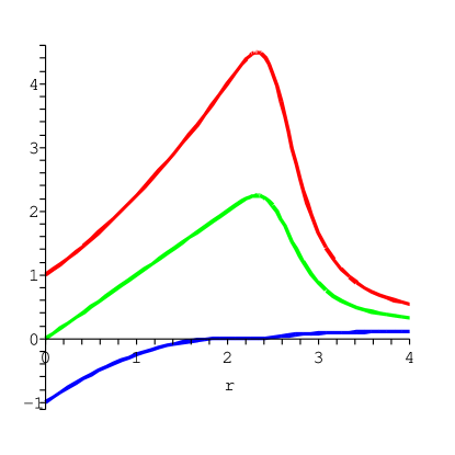
Figure 2: Coordinate speeds for the modified de Sitter (eqn. 10) lightcone: inward light rays, ($v_{\text{in}}$, blue, lowest curve), motion normal to the spacelike time slices ($-\beta$, green, middle curve), and outward light rays ($v_{\text{out}}$, red, highest curve).

This metric surgery has an additional side effect worth noting. For this modified de Sitter metric using Eq. (10) one finds very low inward light velocities in the region just outside $\mathscr{I}^{+}$ as seen in Fig. 3.

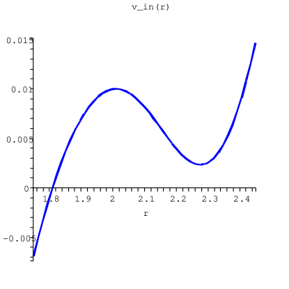
Figure 3: Coordinate speeds inward ($v_{\text{in}}$) for light rays in the modified (eqn. 10) de Sitter metric.

This can lead to fields propagating along the inward side of the lightcone spending very long periods of time in the region $r\approx 2.3$ as illustrated by the world line of a light ray in Fig. 4.

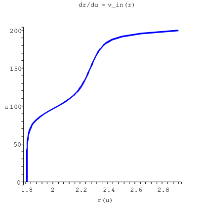
Figure 4: World line of a light ray on the inward side of the light cone in the modified de Sitter metric.

II.2 Maxwell Equations

We take the Maxwell equations in the form given in the DeserFest paper Misner (2006). The quantities involved are all various components of the usual 4-dimensional Maxwell fields $F_{\mu\nu}$ and $\mathcal{F}^{\mu\nu}=\sqrt{-g}g^{\mu\alpha}g^{\nu\beta}F_{\alpha\beta}$. In particular, for any $3+1$ metric of the form Eq. (4) we define,

$$\mathcal{F}^{0i}=\mathcal{D}^{i}\quad,\quad\mathcal{F}^{ij}=[ijk]H_{k}$$ (11a)

and

$$F_{i0}=E_{i}\quad,\quad F_{ij}=[ijk]\mathcal{B}^{k}\quad.$$ (11b)

Here $[ijk]$ is the completely antisymmetric symbol $[ijk]=0,\pm 1$ with $[123]=+1$. The fundamental fields in the formulation are $\mathcal{B}^{i}$ and $\mathcal{D}^{i}$. The constraints read

$$\partial_{i}\mathcal{B}^{i}=0=\partial_{i}\mathcal{D}^{i}\quad.$$ (12)

We need only take regular partial (rather than covariant) derivatives in our formulation of Maxwell’s equations because of judicious use of tensor densities rather than tensors (cf. Exercises 22.8 and 22.9 in Misner et al. (1970)). The resulting fields in Eqs. (12) are each three dimensional vector densities so this equation is three dimensionally covariant. In terms of these primary fields, two auxiliary fields ${E}_{i}$ and ${H}_{i}$ are computed by the formulas

$${E}_{i}=(\alpha/\sqrt{\gamma})\gamma_{ij}\mathcal{D}^{j}+[ijk]\beta^{j}\mathcal{B}^{k}$$ (13a)

and

$${H}_{i}=(\alpha/\sqrt{\gamma})\gamma_{ij}\mathcal{B}^{j}-[ijk]\beta^{j}\mathcal{D}^{k}\quad.$$ (13b)

The evolution equations are then

$$\partial_{0}\mathcal{B}^{i}=-[ijk]\partial_{j}E_{k}$$ (14a)

and

$$\partial_{0}\mathcal{D}^{i}=[ijk]\partial_{j}H_{k}\quad.$$ (14b)

Note that the metric does not appear in Eq. (12) or Eqs. (14), and that the metric quantities which do appear in Eqs. (13) are conformally invariant. This is a first order partial differential equation system in flux conservation form.

II.3 Initial Data

For initial data and some testing purposes we have used the solution of the flat spacetime Maxwell equations employed by Knapp et al. Knapp et al. (2002) and subsequently by Fiske Fiske (2004b). This solution is a wave pulse, which propagates smoothly from $\mathscr{I}^{-}$ through the origin and out to $\mathscr{I}^{+}$. It consists of a toroidal $\mathcal{D}$ field and a poloidal $\mathcal{B}$ field generated from a vector potential, described in Ref. Misner (2006),

$$A=A_{i}dX^{i}=f\sin^{2}\theta d\phi$$ (15)

where

$$\sin^{2}\theta d\phi=\frac{1}{R^{2}}\left(XdY=YdX\right)=\frac{1}{r^{2}}\left(xdy-ydx\right)$$ (16)

and

$$f=\left(\frac{1}{R}-2\lambda U\right)e^{-\lambda U^{2}}-\left(\frac{1}{R}+2\lambda V\right)e^{-\lambda V^{2}}$$ (17)

where the constant $\lambda$ parameterizes the pulse width. In these equations $U\equiv T-R$ and $V\equiv T+R$ are the Minkowski retarded and advanced times, which are then expressed in terms of the compactified coordinates $u$ and $r$ as $U/s=u-2+2/(1+\tfrac{1}{2}r)$ and $V/s=u-2+2/(1-\tfrac{1}{2}r)$. Finally, $\mathcal{B}^{i}$ and $\mathcal{D}^{i}$ are calculated by differentiating this $A$ field. The term containing $e^{-\lambda V^{2}}$ can be smoothly omitted when $r>2$ since all its derivatives vanish at $r=2$, but the term with $e^{-\lambda U^{2}}$ must be retained to preserve the constraints, and we thus have nonzero initial data in the unphysical region $r>2$, i.e. beyond $\mathscr{I}^{+}$, where initial data are not physically meaningful. As the initial pulse is centered at $r=0$, we would ideally like to make it sufficiently narrow so that its amplitude would rapidly taper off and become negligible beyond $r>2$. However, we did not achieve enough resolution to reduce the pulse width to make these unphysical data beyond $r>2$ insignificant.

For all of the simulations described in this paper, we choose $\lambda=1$ (or, equivalently, we measured distances in the uncompactified space in units of $\lambda^{-1/2}$). The pulse width is then $\lambda^{-1/2}$. We also always choose $s=1$ to set the size of the region near the origin where the hyperboloidal slices are somewhat flat. Our results reported below used either $s/L=0$ for the Minkowski case, or $s/L=0.1$ for the de Sitter and modified $[$Eq. 10$]$ de Sitter cases. Thus the $r=\text{constant}$ hypersurfaces were not spacelike for the de Sitter case when $r>2.21$

III Numerics

A key point in our approach to this problem is that we do not require special numerical techniques to handle the compactified spacetime at or within $\mathscr{I}^{+}$. At all interior points, we use second-order, finite-difference approximations to all derivatives. At the computational boundary beyond $\mathscr{I}^{+}$, we use a second-order, one-sided stencil for normal derivatives. We integrate forward in time using the iterated Crank-Nicholson method commonly used in numerical relativity codes Teukolsky (2000).

Our decision to use one-sided differencing at the computational boundary was (in our view) the simplest thing to do. It turns out, however, to be equivalent to the black hole excision boundary conditions first studied in Ref. Shoemaker et al. (2003). To be precise, along a normal to the boundary, the composition of third order extrapolation to a cell just outside the boundary (as used for excision) with second-order center differencing at a cell just inside the boundary gives the same stencil as second-order one-sided differencing at the cell just inside the boundary. This is consistent with our mental picture of excising a region exterior to $\mathscr{I}^{+}$, and reflects the similarity between $\mathscr{I}^{+}$ (at which all characteristics point outward) and an apparent horizon of a black hole (at which all characteristics point inward). As with black hole excision, it is critical for stable and accurate simulations that all light cones at the excision boundary tilt towards the excised region, hence the need for the beyond-$\mathscr{I}^{+}$ metric modification described in Sec. II.1. Without these Eq. (10) modifications, the light cones would point outward only in a neighborhood of $\mathscr{I}^{+}$ which did not extend out to the computational boundary of the cubic grid enclosing $\mathscr{I}^{+}$.

We have verified that our code converges at second order accuracy throughout the physical domain. We paid special attention to the region in the vicinity of $\mathscr{I}^{+}$, and we are satisfied that the code converges there as well. Fig. 5 explicitly shows a two-point convergence test on the constraints over the physical region $r\leq 2$, which are seen to be second-order convergent to zero and nearly constant.

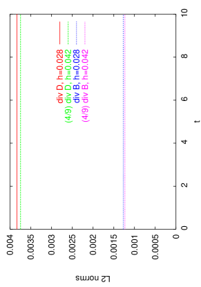
Figure 5: The L2 norms (over the region $r\leq 2$) of the constraints plotted vs. time. The higher resolution data is multiplied by the factor appropriate to demonstrate second order convergence. The initial values arise from $\mathcal{B}$ and $\mathcal{D}$ fields which are exact analytic solutions of the constraints, evaluated at the grid points and then differenced to form the constraints.

IV Results

When evolving with the original, conformal, de Sitter metric given in Eq. (1), large errors eventually appear near the computational grid boundary, grow exponentially in time, and propagate inside $\mathscr{I}^{+}$. This problem was slightly worse when the cosmological constant was omitted. These cataclysmic errors originated at the grid boundary which in these cases was not a spacelike hypersurface for which excisions (at apparent horizons) were designed. As anticipated in Sec. II.1 we proceeded to artificially tilt the lightcones outwards beyond $\mathscr{I}^{+}$ to make the grid boundaries spacelike.

Fig. 6 shows a spacetime view of the $z$ component of the magnetic field for an evolution using the modified (eqn. 10) de Sitter metric.

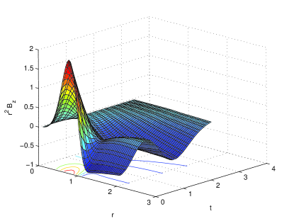
Figure 6: A spacetime graph of $r^{2}\mathcal{B}^{z}$. Notice that the wave passes through $\mathscr{I}^{+}$, located at $r=2$ in our coordinate system.

In order to make clear that the wave is cleanly passing through $\mathscr{I}^{+}$ through the course of the evolution, we have multiplied the field by $r^{2}$, making the scale of the field comparable at the origin and at $\mathscr{I}^{+}$. This can be seen in a more local way in Fig. 7,

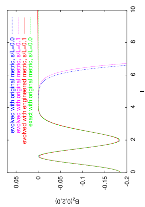
Figure 7: The time evolution of $\mathcal{B}^{z}$ at a point on $\mathscr{I}^{+}$. We show both a numerical solution generated by our code using the modified de Sitter (engineered lightcones beyond $\mathscr{I}^{+}$) and the analytic solution with zero cosmological constant. The close agreement of the lines suggests that we are able to accurately capture the behavior of the fields as they pass through $\mathscr{I}^{+}$. Other numerical evolutions based on the original (compactified, analytically continued) Minkowski metric ($s/L=0.0$) and the similar de Sitter metric ($s/L=0.1$), for which the grid boundaries were not spacelike, fail after $t\equiv u=4$.

which shows the time evolution of $\mathcal{B}^{z}$ at a single point on $\mathscr{I}^{+}$, for four cases. One is the analytic value of the field (in extended Minkowski spacetime) for comparison. The two cases which failed to maintain vanishing fields in the wake of the outgoing pulse correspond to the two (Minkowski and de Sitter) metrics for which the modifications needed to make the grid boundaries beyond $\mathscr{I}^{+}$ spacelike $[$Eq. (10)$]$ were not implemented.

Note that the analytic solution is with zero cosmological constant, whereas the numerically evolved solution is with finite cosmological constant, and yet the waveforms coincide. This phenomenon can be understood as follows. Because, as pointed out in Sec. II.1, the outgoing speed of light is the same in either case, the phase of outgoing waves can be said to be independent of a cosmological constant here. Further, since by construction the initial wave pulse is identical in our Minkowski and de Sitter simulations, by conservation of energy the wave amplitudes at $\mathscr{I}^{+}$ are expected to be commensurate.

These results show that many desired aims of this approach are achieved. Waves propagate smoothly through $\mathscr{I}^{+}$ and no difficulties appear to arise in the neighborhood of $\mathscr{I}^{+}$ The compactified hyperboloidal slices allow waves to appear at $\mathscr{I}^{+}$ a very short computational time after they originate in the central region. No modifications were needed to integration algorithms designed for conventional spacelike Cauchy slicings. The excision at a cubic computational boundary, however, only maintained acceptable behavior for a time several times the pulse width, and ultimately led to behaviors in the unphysical region beyond $\mathscr{I}^{+}$ which became intolerable. An example is given in Fig A2 where the constraint violations beyond $\mathscr{I}^{+}$ are seen eventually to increase exponentially. In addition, by using analytically constructed initial values satisfying the constraints, we had to accept nonzero initial conditions in the unphysical region $r>2$ beyond $\mathscr{I}^{+}$, and the subsequent evolution of these fields complicated the computation beyond $\mathscr{I}^{+}$.

We believe that further developments of Cauchy evolutions with compactified hyperboloidal slicings and artificial cosmology should be done with the computational/excision boundary a spherical hypersurface at or modestly beyond $\mathscr{I}^{+}$. The means for doing this have been developed, e.g. Kidder et al. (2005); Thornburg (2004); Lehner et al. (2005); Diener et al. (2005). Then the possibility remains open that well posed wave equations could run indefinitely. As explained in the supplementary material (Appendix), here we did not use the differential equations from Sec. VI of Misner (2005) as our lightcone engineering (see Sec. II.1) beyond $\mathscr{I}^{+}$ makes the constraints there increase exponentially even from analytic arguments. A spherical boundary could be spacelike at $r>2$ without the need for such artificial tilting of the lightcones, and thus allow the use of the formulation (Misner, 2005, Equations 26) where constraints evolve causally.

Appendix A Auxiliary material

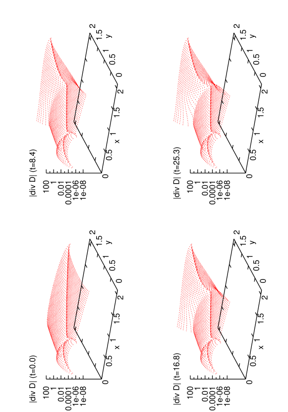
Figure A1: Samples of the time evolution of the constraint violation $|\text{div}\mathcal{D}|$ at $z=0$ within our comptational cube $|x^{i}|<2.1$ whose edges are at $r=2.97$ .

This section is mainly a collection of graphs which illustrate properties that are merely asserted in the main article.

A.1 Constraints

Even when the modified de Sitter metric is used, the solution in the unphysical region deteriorates as shown in Figs. A1 and A2.

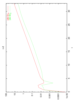
Figure A2: The time evolution of an L2 norm of the constraint violations over the unphysical region $r>2$ beyond $\mathscr{I}^{+}$ within our computational cube $|x^{i}|<2.1$ whose corners are at $r=3.64$ .

In spite of these problems, the field at $\mathscr{I}^{+}$ remains zero after the wave pulse passes (Fig. 7) for a moderately long time, which can be lengthened by using higher resolution. See Fig. A3.

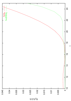
Figure A3: A continuation of the test wave pulse to later times at $\mathscr{I}^{+}$.

Better control of the constraints should be possible using the equation

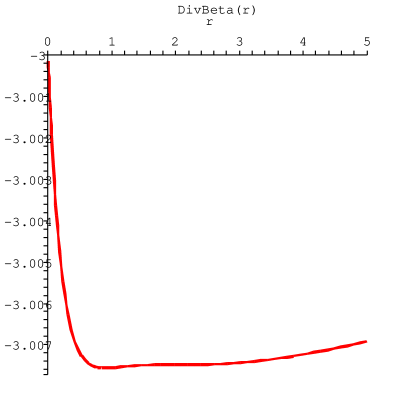
Figure A4: The damping factor for constraints in the de Sitter metric.

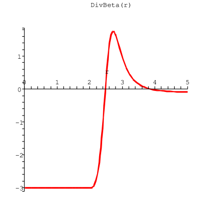
Figure A5: The damping factor for constraints in the modified de Sitter metric. Where $\text{div}\beta$ is positive, the constraints should grow exponentially at the plotted e-folding rate.

system (Misner, 2005, Equations 26) where the constraints propagate inside the lightcone and damp at a rate $-\partial_{i}\beta^{i}$. However this is damping only for the Minkowski or de Sitter metrics as seen in Fig. A4 and becomes anti-damping for our modification of the de Sitter metric (see Fig. A5 ) which makes our cubic grid boundaries spacelike.

A.2 Initial conditions beyond $\mathscr{I}^{+}$.

A second reason which makes the use of the full cubic grid (rather than only a region inside a spherical boundary such as $r=2$ or $r=2.1$) inappropriate for numerical computation is the need for initial values beyond $\mathscr{I}^{+}$, that is beyond $r=2$, which is $R=\infty$.

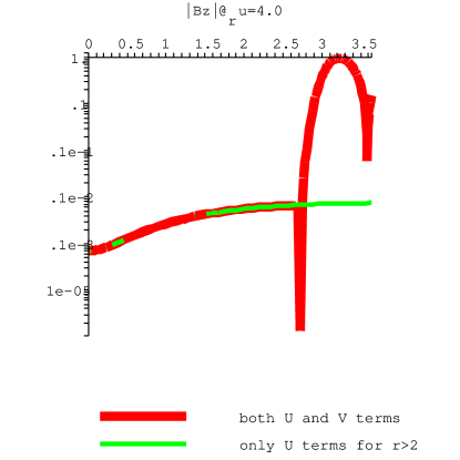
Figure A6: For the analytic solution in Minkowski spacetime: The magnetic field at $z=0$ after the pulse from Fig 7 has exited the computational grid.

With a spherical excision boundary and causal propagation of all modes, there is less room for bad initial conditions to intrude, and better reason to think that even poor initial conditions would be quickly flushed out of the computational domain. We have simply used as initial conditions the formulas for $\mathcal{B}$ and $\mathcal{D}$ as computed from equations (15) through (17) extended analytically by the coordinate transformation from $TSYZ$ to $uxyz$ of equations (2). As a solution of the Maxwell equations in the Minkowski metric, these formulae give substantial activity in the $r>2$ region, as seen in Fig.A6. In that Figure one solution has been modified by smoothly deleting the terms involving $\exp{-\lambda V^{2}}$ for $r\geq 2$ which is possible since $V/s=u-2+2/(1-\tfrac{1}{2}r)$ becomes infinite at $r=2$. However the pulse seen moving inward from beyond the grid will have depended upon initial conditions far outside $r=3.64=2.1\sqrt{3}$ which was the limit of our grid. Our initial data, however, are not evolved using the Minkowski metric, but usually with the de Sitter or modified de Sitter metrics, where the decomposition into ingoing and outgoing parts of the initial conditions will differ seriously from the Minkowski case, especially well beyond $\mathscr{I}^{+}$. Thus we can understand that different, but equally visible, activity could occur in the $r>2$ region which would be actually solving the given differential equations but be unrelated to the physical activity in the region $r\leq 2$. This appears to be occuring in the numerical results (modified de Sitter for which no analytic solution is available) shown in Fig. A7.

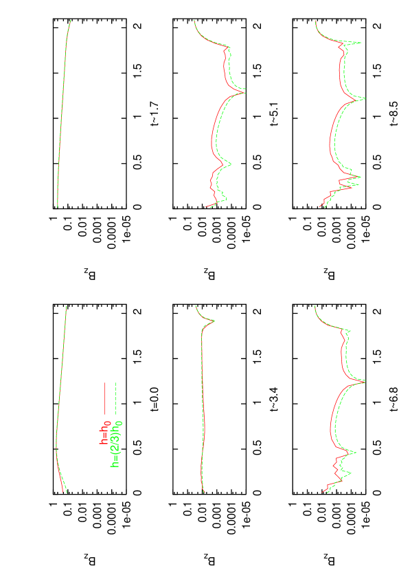
Figure A7: A field component plotted along a line $z=0,x=1$ parallel to the $y$-axis. At the grid limit $y=2.1$ one has $r=2.33$, while $\mathscr{I}^{+}$ is met at $y=1.73$. Inside $\mathscr{I}^{+}$ the field values appear to be convergent to zero after $u=4$, while in the region beyond $y=1.85$ or $r=2.1$ a slowly moving pulse appears to remain independent of the selected resolution.