Method of comparison equations for cosmological perturbations

Abstract

We apply the method of comparison equations to study cosmological perturbations during inflation, obtaining the full power spectra of scalar and tensor perturbations to first and to second order in the slow-roll parameters. We compare our results with those derived by means of other methods, in particular the Green’s function method and the improved WKB approximation, and find agreement for the slow-roll structure. The method of comparison equations, just as the improved WKB approximation, can however be applied to more general situations where the slow-roll approximation fails.

1 Introduction

Anisotropies in the cosmic microwave background (CMB) radiation and inhomogeneities in the large scale structures of the Universe have nowadays become a fundamental tool to study the early universe [1]. Present and future data will allow us to discriminate among different inflationary models in the near future. For this reason, the comparison of observations with inflationary models requires theoretical advances in the predictions of the power spectrum of primordial perturbations beyond the lowest order in the slow-roll parameters $\epsilon_{i}$’s, first obtained by Stewart and Lyth [2] (their definitions will be recalled in Section 3).

An analytic form for the full inflationary power spectra to second order in the slow-roll parameters was first obtained through the Green’s function method (GFM henceforth) in Ref. [3]. In this way a characterization of the power spectrum to second order in the slow-roll parameters was given which was not just derived from the running of the spectral index (whose leading order is precisely ${\cal O}(\epsilon^{2})$ [4]). An equivalent second order characterization has been recently obtained by means of the improved WKB approximation of Refs. [5, 6], which extended to second order in the slow-roll parameters previous results based on a more standard WKB approach [7, 8]. The WKB approximation has confirmed the structure of the second order power spectra found with the GFM, within a numerical difference in the ${\cal O}(\epsilon^{2})$ coefficients of $5\,\%$ at most [5]. Compared with the GFM, the WKB approximation has the additional advantage that the slow-roll parameters do not have to be constant in time [6] and can therefore be applied to a wider class of inflationary models.

The purpose of this paper is to illustrate the use of the method of comparison equations (MCE in brief) [9, 10, 11] to predict inflationary power spectra. We shall see that this method yields exact results for the case of constant slow-roll parameters (e.g. power-law inflation) and polynomial structures to second order in the $\epsilon_{i}$’s in agreement with the GFM and WKB approximation. The MCE however has the advantage of being more accurate to lowest (leading) order, whereas other methods (namely, the WKB [7], improved WKB [8] and GFM [3]) reach a similar accuracy to next-to-leading order. We shall also discuss cases for which our present method appears more flexible than the slow-roll approximation.

In the next Section we briefly review the general MCE and in Section 3 the theory of cosmological perturbations. We then apply the MCE to cosmological perturbations in Section 4 where we also analyze the error around the “turning point” in detail. In Section 5 we analyze power-law inflation, chaotic inflation and the arctan model; we expand our general results to second slow-roll order and compare with analogous results obtained with the GFM. We finally comment on our results in Section 6. Some more technical details are given in two Appendices.

2 Method of comparison equations

Let us briefly review the MCE (the name is due to Dingle [10]). It was independently introduced in Refs. [9, 10] and applied to wave mechanics by Berry and Mount in Ref. [11]. The standard WKB approximation and its improvement by Langer [12] are just particular cases of this method and, recently, its connection with the Ermakov-Pinney equation was also studied [13].

Let us consider the second-order differential equation

$$\left[\frac{{\mbox{${\rm d}$}}^{2}}{{\mbox{${\rm d}$}}x^{2}}+\omega^{2}(x)\right]\,\chi(x)=0\ ,$$ (1)

where $\omega^{2}$ is a (not necessarily positive) “potential” (or “frequency”), and suppose that we know an exact solution to a similar second-order differential equation,

$$\left[\frac{{\mbox{${\rm d}$}}^{2}}{{\mbox{${\rm d}$}}\sigma^{2}}+\Theta^{2}(\sigma)\right]\,U(\sigma)=0\ ,$$ (2)

where $\Theta$ is the “comparison function”. One can then represent an exact solution of Eq. (1) in the form

$$\chi(x)=\left(\frac{{\mbox{${\rm d}$}}\sigma}{{\mbox{${\rm d}$}}x}\right)^{-1/2}\,U(\sigma)\ ,$$ (3)

provided the variables $x$ and $\sigma$ are related by

$$\omega^{2}(x)\!=\!\left(\frac{{\mbox{${\rm d}$}}\sigma}{{\mbox{${\rm d}$}}x}\right)^{2}\Theta^{2}(\sigma)-\left(\frac{{\mbox{${\rm d}$}}\sigma}{{\mbox{${\rm d}$}}x}\right)^{1/2}\frac{{\mbox{${\rm d}$}}^{2}}{{\mbox{${\rm d}$}}x^{2}}\left(\frac{{\mbox{${\rm d}$}}\sigma}{{\mbox{${\rm d}$}}x}\right)^{-1/2}\ .$$ (4)

Eq. (4) can be solved by using some iterative scheme, in general cases [13, 14] or for specific problems [15, 16]. If we choose the comparison function sufficiently similar to $\omega$, the second term in the right hand side (r.h.s.) of Eq. (4) will be negligible with respect to the first one, so that

$$\omega^{2}(x)\simeq\left(\frac{{\mbox{${\rm d}$}}\sigma}{{\mbox{${\rm d}$}}x}\right)^{2}\Theta^{2}(\sigma)\ .$$ (5)

On selecting a pair of values $x_{0}$ and $\sigma_{0}$ such that $\sigma_{0}=\sigma(x_{0})$, the function $\sigma(x)$ can be implicitly expressed as

$$-\xi(x)\equiv\int_{x_{0}}^{x}\sqrt{\pm\,\omega^{2}(y)}\,{\mbox{${\rm d}$}}\,y\simeq\int_{\sigma_{0}}^{\sigma}\sqrt{\pm\,\Theta^{2}(\rho)}\,{\mbox{${\rm d}$}}\,\rho\ ,$$ (6)

where the signs are chosen conveniently . The result in Eq. (3) leads to a uniform approximation for $\chi(x)$, valid in the whole range of the variable $x$, including “turning points” . The similarity between $\Theta$ and $\omega$ is clearly very important in order to implement this method.

3 Cosmological perturbations

Let us begin by recalling that scalar (density) and tensor (gravitational wave) fluctuations on a flat Robertson-Walker background with scale factor $a$

$$\mbox{${\rm d}$}s^{2}=a^{2}\,\left(-\mbox{${\rm d}$}\eta^{2}+\mbox{${\rm d}$}r^{2}+r^{2}\mbox{${\rm d}$}\Omega^{2}\right)\ ,$$ (7)

are given respectively by $\mu=\mu_{\rm S}\equiv a\,Q$ and $\mu=\mu_{\rm T}\equiv a\,h$, where $Q$ is the Mukhanov variable [17, 18] and $h$ the amplitude of the two polarizations of gravitational waves [19, 20]. The functions $\mu$ must satisfy the one-dimensional Schrödinger-like equation

$$\left[\frac{{\mbox{${\rm d}$}}^{2}}{{\mbox{${\rm d}$}}\eta^{2}}+\Omega^{2}(k,\eta)\right]\,\mu=0\ ,$$ (8)

together with the initial condition (corresponding to a Bunch-Davies vacuum)

$$\lim_{\frac{k}{a\,H}\rightarrow+\infty}\mu(k,\eta)\simeq\frac{{\rm e}^{-i\,k\,\eta}}{\sqrt{2\,k}}\ .$$ (9)

In the above $\eta$ is the conformal time (derivatives with respect to it will be denoted by primes), $k$ the wave-number, $H=a^{\prime}/a^{2}$ the Hubble parameter and

$$\Omega^{2}(k,\eta)\equiv k^{2}-\frac{z^{\prime\prime}}{z}\ ,$$ (10)

where $z=z_{\rm S}\equiv a^{2}\,\phi^{\prime}/H$ for scalar and $z=z_{\rm T}\equiv a$ for tensor perturbations ($\phi$ is the homogenous inflaton). The dimensionless power spectra of scalar and tensor fluctuations are then given by

$$\mathcal{P}_{\zeta}\equiv\displaystyle\frac{k^{3}}{2\,\pi^{2}}\,\left|\frac{\mu_{\rm S}}{z_{\rm S}}\right|^{2}\ ,\ \ \ \ \mathcal{P}_{h}\equiv\displaystyle\frac{4\,k^{3}}{\pi^{2}}\,\left|\frac{\mu_{\rm T}}{z_{\rm T}}\right|^{2}$$ (11a)

and the spectral indices and runnings by

$$n_{\rm S}-1\equiv\left.\displaystyle\frac{\mbox{${\rm d}$}\ln\mathcal{P}_{\zeta}}{\mbox{${\rm d}$}\ln k}\right|_{k=k_{*}}\ ,\ \ \ n_{\rm T}\equiv\left.\displaystyle\frac{\mbox{${\rm d}$}\ln\mathcal{P}_{h}}{\mbox{${\rm d}$}\ln k}\right|_{k=k_{*}}$$ (11b)

$$\alpha_{\rm S}\equiv\left.\frac{\mbox{${\rm d}$}^{2}\ln\mathcal{P}_{\zeta}}{(\mbox{${\rm d}$}\ln k)^{2}}\right|_{k=k_{*}}\ ,\ \ \ \alpha_{\rm T}\equiv\left.\frac{\mbox{${\rm d}$}^{2}\ln\mathcal{P}_{h}}{(\mbox{${\rm d}$}\ln k)^{2}}\right|_{k=k_{*}}$$ (11c)

where $$k_{*} k=k_{*}$$ is an arbitrary pivot scale. We also define the tensor-to-scalar ratio at as

$$R\equiv\left.\frac{\mathcal{P}_{h}}{\mathcal{P}_{\zeta}}\right|_{k=k_{*}}\ .$$ (11d)

Finally, in the following we shall often make use of the hierarchy of horizon flow functions (HFF in short, also referred to as slow-roll parameters) $\epsilon_{i}$’s defined by [21]

$$\epsilon_{1}\equiv-\frac{\dot{H}}{H^{2}}\ ,\quad\quad\epsilon_{n+1}\equiv\frac{\dot{\epsilon}_{n}}{H\,\epsilon_{n}}\quad n\geq 1$$ (11l)

where dots denote derivatives with respect to the cosmic time $\mbox{${\rm d}$}t=a\,\mbox{${\rm d}$}\eta$.

4 MCE and cosmological perturbations

In order to apply the MCE to cosmological perturbations, we shall start from the same equation as was used with the improved WKB method in Refs. [7, 8], to which we refer for more details. We recall here that the WKB approximation can be more effectively applied after the following redefinitions of the wave-function and variable,

$$\chi=(1-\epsilon_{1})^{1/2}\,{\rm e}^{-x/2}\,\mu$$ (11ma)

$$x=\ln\left(\frac{k}{H\,a}\right)\ .$$ (11mb)

This yields an equation of the form (1) with the “frequency” $\Omega(k,\eta)$ of Eq. (8) replaced by

$$\omega^{2}(x)=\frac{{\rm e}^{2\,x}}{\left[1-\epsilon_{1}(x)\right]^{2}}-\nu^{2}(x)\ ,$$ (11mn)

with $\nu^{2}(x)$ given, respectively for scalar and tensor perturbations, by

$$\!\!\!\!\!\!\!\!\!\!\!\!\!\!\!\!\!\!\!\!\!\!\!\!\!\nu_{\rm S}^{2}(x) = \frac{1}{4}\,\left(\frac{3-\epsilon_{1}}{1-\epsilon_{1}}\right)^{2}+\frac{(3-2\,\epsilon_{1})\,\epsilon_{2}}{2\,(1-\epsilon_{1})^{2}}+\frac{(1-2\,\epsilon_{1})\,\epsilon_{2}\,\epsilon_{3}}{2\,(1-\epsilon_{1})^{3}}+\frac{(1-4\,\epsilon_{1})\,\epsilon_{2}^{2}}{4\,(1-\epsilon_{1})^{4}}$$ (11moa)

$$\!\!\!\!\!\!\!\!\!\!\!\!\!\!\!\!\!\!\!\!\!\!\!\!\!\nu_{\rm T}^{2}(x) = \frac{1}{4}\,\left(\frac{3-\epsilon_{1}}{1-\epsilon_{1}}\right)^{2}-\frac{\epsilon_{1}\,\epsilon_{2}}{2\,(1-\epsilon_{1})^{2}}-\frac{\epsilon_{1}\,\epsilon_{2}\,\epsilon_{3}}{2\,(1-\epsilon_{1})^{3}}-\frac{(2+\epsilon_{1})\,\epsilon_{1}\,\epsilon_{2}^{2}}{4\,(1-\epsilon_{1})^{4}}\ ,$$ (11mob)

where we omit the dependence on $x$ in the $\epsilon_{i}$ for the sake of brevity. The point $x=x_{0}$ where the frequency vanishes, $\omega(x_{0})=0$ (i.e. the classical “turning point”), is given by the expression

$$x_{0}=\ln\left[\bar{\nu}\,\left(1-\bar{\epsilon}_{1}\right)\right]\ ,$$ (11mop)

where we have defined $\bar{\nu}\equiv\nu(x_{0})$ and $\bar{\epsilon}_{1}\equiv\epsilon_{1}(x_{0})$. We now choose the comparison function

$$\Theta^{2}(\sigma)=\frac{{\rm e}^{2\,\sigma}}{(1-\bar{\epsilon}_{1})^{2}}-\bar{\nu}^{2}\ ,$$ (11moq)

and note that then $\sigma_{0}=x_{0}$. Solutions to Eq. (1) can now be expressed, by means of Eqs. (2), (5) and (11moq), as

$$\chi_{\pm}(x)\simeq\sqrt{\frac{\Theta(\sigma)}{\omega(x)}}\,J_{\pm\bar{\nu}}\left(\frac{{\rm e}^{\sigma}}{1-\bar{\epsilon}_{1}}\right)\ ,$$ (11mor)

where the $J$’s are Bessel functions [22], and the initial condition (9) can be satisfied by taking a linear combination of them. However, in contrast with the WKB method [7, 8] and as we pointed out in Section 2, MCE solutions need not be matched at the turning point, since the functions (11mor) are valid solutions for the whole range of the variable $x$. Eq. (6) at the end of inflation, $x=x_{\rm f}$, becomes

$$\xi(x_{\rm f}) \simeq -\Theta(\sigma_{\rm f})-\frac{\bar{\nu}}{2}\,\ln\left[\frac{\bar{\nu}-\Theta(\sigma_{\rm f})}{\bar{\nu}+\Theta(\sigma_{\rm f})}\right]$$ (11mos)

$$\simeq -\bar{\nu}\,\left[1+\ln\left(\frac{{\rm e}^{\sigma_{\rm f}}}{1-\bar{\epsilon}_{1}}\right)-\ln\left(2\,\bar{\nu}\right)\right]\ ,$$

where the super-horizon limit $x_{\rm f}\ll x_{0}$ ($\sigma_{\rm f}\to-\infty$) has been taken in the second line. One then has

$$\frac{{\rm e}^{\sigma_{\rm f}}}{1-\bar{\epsilon}_{1}}\simeq\frac{2\,\bar{\nu}}{\rm e}\,{\rm exp}\left[-\frac{\xi(x_{\rm f})}{\bar{\nu}}\right]\ .$$ (11mot)

Finally, on using Eq. (11mot), we obtain the general expressions for the power spectra to leading MCE order,

$${\cal P}_{\zeta} = \left[\frac{H^{2}}{\pi\,\epsilon_{1}\,m_{\rm Pl}^{2}}\left(\frac{k}{a\,H}\right)^{3}\frac{{\rm e}^{2\,\xi_{\rm S}}}{\left(1-\epsilon_{1}\right)\,\omega_{\rm S}}\right]_{x=x_{\rm f}}g_{\rm S}(x_{0})$$ (11moua)

$${\cal P}_{h} = \left[\frac{16\,H^{2}}{\pi\,m_{\rm Pl}^{2}}\,\left(\frac{k}{a\,H}\right)^{3}\,\frac{{\rm e}^{2\,\xi_{\rm T}}}{\left(1-\epsilon_{1}\right)\,\omega_{\rm T}}\right]_{x=x_{\rm f}}g_{\rm T}(x_{0})\ ,$$ (11moub)

where $$m_{\rm Pl}$$ is the Planck mass and the quantities inside the square brackets are evaluated in the super-horizon limit, whereas the functions

$$g(x_{0})\equiv\frac{\pi\,e^{2\,\bar{\nu}}\,\bar{\nu}^{1-2\,\bar{\nu}}}{\left[1-\cos\left(2\,\pi\,\bar{\nu}\right)\right]\,\left[\Gamma\left(1-\bar{\nu}\right)\right]^{2}}\ ,$$ (11mouc)

describe corrections that just depend on quantities evaluated at the turning point and represent the main result of the MCE applied to cosmological perturbations . The expression in Eq. (11mouc) is obtained by simply making use of the approximate solutions (11mor) and their asymptotic expansion at $x\to\infty$ to impose the initial conditions (9). In the WKB calculations [5, 6, 8] one finds a similar factor but, in that case, using the Bessel functions of order $1/3$ leads to a large error in the amplitudes. The MCE instead uses Bessel functions of order $\bar{\nu}$, with $\bar{\nu}=3/2$ to leading order in the HFF (i.e. the right index for the de Sitter model), which yields a significantly better value for the amplitudes of inflationary spectra.

The MCE allows one to compute approximate perturbation modes with errors in the asymptotic regions (i.e. in the sub- and super-horizon limits) which are comparable with those of the standard (or improved) WKB approximation [7, 8]. Since these methods usually give large errors at the turning point [8] (which produce equally large errors in the amplitude of the power spectra) it will suffice to estimate the error at the turning point in order to show that the MCE is indeed an improvement. To leading order (that is, on using the approximate solution (11mor)), the MCE gives an error at the turning point of the second order in the HFF, which means that we have a small error in the amplitudes of the power spectra. Unfortunately, this error remains of second order in the HFF also for next-to-leading order in the MCE. We shall see this by applying Dingle’s analysis [10] for linear frequencies to our case (11mn). We start by rewriting Eq. (4) as

$$\left\{\omega^{2}-\sigma_{1}^{2}\,\left[\frac{{\rm e}^{2\,\sigma}}{(1-\bar{\epsilon}_{1})^{2}}-\bar{\nu}^{2}\right]\right\}+\left[\frac{3}{4}\,\frac{\sigma_{2}^{2}}{\sigma_{1}^{2}}-\frac{1}{2}\,\frac{\sigma_{3}}{\sigma_{1}}\right]=0\ ,$$ (11mouv)

where we dropped the $x$ dependence in $\omega$ and $\sigma$ and the order of the derivatives is given by their subscripts ($\sigma_{1}\equiv\mbox{${\rm d}$}\sigma/\mbox{${\rm d}$}x$, $\omega_{1}^{2}\equiv\mbox{${\rm d}$}\omega^{2}/\mbox{${\rm d}$}x$, etc.). Note that the term in square brackets is the error obtained on using the solutions (11mor). We then evaluate Eq. (11mouv) and its subsequent derivatives at the turning point (i.e. at $x=x_{0}$),

$$\!\!\!\!\!\!\!\!\!\!\!\!\!\!\!\!\!\!\!\!\!\!\!\!\!\!\!\!\!\!\!\!\!\!\!\!\!\!\!\!\left\{\omega^{2}-\sigma_{1}^{2}\,\Theta^{2}\left(\sigma\right)\right\}+\left[\frac{3}{4}\,\frac{\sigma_{2}^{2}}{\sigma_{1}^{2}}-\frac{1}{2}\,\frac{\sigma_{3}}{\sigma_{1}}\right]=0$$ (11mouwa)

$$\!\!\!\!\!\!\!\!\!\!\!\!\!\!\!\!\!\!\!\!\!\!\!\!\!\!\!\!\!\!\!\!\!\!\!\!\!\!\!\!\left\{\omega^{2}_{1}-2\,\sigma_{2}\,\sigma_{1}\,\Theta^{2}\left(\sigma\right)-\frac{2\,{\rm e}^{2\,\sigma}\,\sigma_{1}^{3}}{\left(1-\bar{\epsilon}_{1}\right)^{2}}\right\}+\left[2\,\frac{\sigma_{3}\,\sigma_{2}}{\sigma_{1}^{2}}-\frac{3}{2}\,\frac{\sigma_{2}^{3}}{\sigma_{1}^{3}}-\frac{1}{2}\,\frac{\sigma_{4}}{\sigma_{1}}\right]=0$$ (11mouwb)

$$\left\{\omega^{2}_{2}-2\,\left(\sigma_{3}\,\sigma_{1}+\sigma_{2}^{2}\right)\,\Theta^{2}\left(\sigma\right)-\frac{2\,\sigma_{1}^{2}\,{\rm e}^{2\,\sigma}}{\left(1-\bar{\epsilon}_{1}\right)^{2}}\,\left(2\,\sigma_{1}^{2}+5\,\sigma_{2}\right)\right\}$$

$$+\left[\frac{9}{2}\,\frac{\sigma_{2}^{4}}{\sigma_{1}^{4}}-\frac{17}{2}\frac{\sigma_{3}\,\sigma_{2}^{2}}{\sigma_{1}^{3}}+\frac{5}{2}\,\frac{\sigma_{4}\,\sigma_{2}}{\sigma_{1}^{2}}+2\,\frac{\sigma_{3}^{2}}{\sigma_{1}^{2}}-\frac{1}{2}\,\frac{\sigma_{5}}{\sigma_{1}}\right]=0$$ (11mouwc)

$$\left\{\omega^{2}_{3}-2\,\left(\sigma_{4}\,\sigma_{1}+3\,\sigma_{2}\,\sigma_{3}\right)\,\Theta^{2}\left(\sigma\right)-\frac{2\,\sigma_{1}\,{\rm e}^{2\,\sigma}}{\left(1-\bar{\epsilon}_{1}\right)^{2}}\,\left(4\,\sigma_{1}^{4}+18\,\sigma_{2}\,\sigma_{1}^{2}+7\,\sigma_{3}\,\sigma_{1}+12\,\sigma_{2}^{2}\right)\right\}$$

$$+\left[\frac{87}{2}\,\frac{\sigma_{3}\,\sigma_{2}^{3}}{\sigma_{1}^{4}}-18\,\frac{\sigma_{2}^{5}}{\sigma_{1}^{5}}-\frac{27}{2}\,\frac{\sigma_{4}\,\sigma_{2}^{2}}{\sigma_{1}^{3}}-21\,\frac{\sigma_{3}^{2}\,\sigma_{2}}{\sigma_{1}^{3}}+3\,\frac{\sigma_{5}\,\sigma_{2}}{\sigma_{1}^{2}}+\frac{13}{2}\,\frac{\sigma_{3}\,\sigma_{4}}{\sigma_{1}^{2}}-\frac{1}{2}\,\frac{\sigma_{6}}{\sigma_{1}}\right]=0\ ,$$ (11mouwd)

where $\Theta^{2}\left(\sigma\right)$ was defined in Eq. (11moq) and we omit two equations for brevity. In order to evaluate the error at the turning point

$$\Delta_{\rm TP}=\left[\frac{3}{4}\,\frac{\sigma_{2}^{2}}{\sigma_{1}^{2}}-\frac{1}{2}\,\frac{\sigma_{3}}{\sigma_{1}}\right]_{x=x_{0}}\ ,$$ (11mouwx)

we ignore the terms in square brackets and equate to zero the expressions in the curly brackets in Eqs. (11mouwa)-(11mouwd) and so on. This leads to

$$\!\!\!\!\!\!\!\!\!\!\!\!\!\!\!\!\!\!\!\!\!\!\!\!\!\!\!\!\!\!\!\!\!\!\!\!\!\!\sigma \!=\! \ln\left[\left(1-\bar{\epsilon}_{1}\right)\,\bar{\nu}\right]$$ (11mouwya)

$$\!\!\!\!\!\!\!\!\!\!\!\!\!\!\!\!\!\!\!\!\!\!\!\!\!\!\!\!\!\!\!\!\!\!\!\!\!\!\sigma_{1} \!=\! \left(\frac{\omega^{2}_{1}}{2\,\bar{\nu}^{2}}\right)^{1/3}$$ (11mouwyb)

$$\!\!\!\!\!\!\!\!\!\!\!\!\!\!\!\!\!\!\!\!\!\!\!\!\!\!\!\!\!\!\!\!\!\!\!\!\!\!\sigma_{2} \!=\! \frac{1}{5\,\left(2\,\bar{\nu}^{2}\right)^{1/3}}\left[\frac{\omega^{2}_{2}}{\left(\omega^{2}_{1}\right)^{2/3}}-\left(2\,\frac{\omega^{2}_{1}}{\bar{\nu}}\right)^{2/3}\right]$$ (11mouwyc)

$$\!\!\!\!\!\!\!\!\!\!\!\!\!\!\!\!\!\!\!\!\!\!\!\!\!\!\!\!\!\!\!\!\!\!\!\!\!\!\sigma_{3} \!=\! -\frac{6\left(2^{1/3}\,\omega^{2}_{2}\right)^{2}}{175\,\left(\bar{\nu}^{2/5}\,\omega^{2}_{1}\right)^{5/3}}-\frac{3\cdot 2^{1/3}\,\omega^{2}_{2}}{25\,\left(\bar{\nu}^{4}\,\omega^{2}_{1}\right)^{1/3}}+\frac{16\,\omega^{2}_{1}}{175\,\bar{\nu}^{2}}+\frac{\omega^{2}_{3}}{7\left(2^{1/2}\,\bar{\nu}\,\omega^{2}_{1}\right)^{2/3}}\ ,$$ (11mouwyd)

and similar expressions for $\sigma_{4}$, $\sigma_{5}$, and $\sigma_{6}$ which we again omit for brevity. On inserting Eqs. (11mn), (11moa) and (11mob) in the above expressions, we find the errors to leading MCE order

$$\Delta^{(0)}_{\rm TP,S} = -\frac{32}{315}\,\epsilon_{1}\,\epsilon_{2}-\frac{22}{315}\,\epsilon_{2}\,\epsilon_{3}$$ (11mouwyza)

$$\Delta^{(0)}_{\rm TP,T} = -\frac{32}{315}\,\epsilon_{1}\,\epsilon_{2}\ ,$$ (11mouwyzb)

for scalar and tensor modes respectively.

On iterating this procedure we can further obtain the errors for the next-to-leading MCE order $\Delta^{(1)}_{\rm TP}$. We first compute next-to-leading solutions to Eqs. (11mouwa)-(11mouwd) and so on by inserting the solutions found to leading order for $\sigma_{1},\sigma_{2},\ldots,\sigma_{6}$ into the corrections (i.e. the square brackets) and into all terms containing $\Theta^{2}(\sigma)$ [10]. This leads to

$$\Delta^{(1)}_{\rm TP,S} = -\frac{31712}{331695}\,\epsilon_{1}\,\epsilon_{2}-\frac{21598}{331695}\,\epsilon_{2}\,\epsilon_{3}$$ (11mouwyzaaa)

$$\Delta^{(1)}_{\rm TP,T} = -\frac{31712}{331695}\,\epsilon_{1}\,\epsilon_{2}\ ,$$ (11mouwyzaab)

which show that the next-to-leading MCE solutions lead to an error of second order in the HFF, too. We suspect that this remains true for higher MCE orders, since there is no a priori relation between the MCE and the slow-roll expansions. Let us however point out that the above expressions were obtained without performing a slow-roll expansion and therefore do not require that the $\epsilon_{i}$ be small.

5 Applications

In this section we apply the formalism developed in the previous section to some models of inflation. We shall expand our general expressions (11moua)-(11mouc) to second order in the HFF and compare them with other approximation methods used in the literature.

5.1 Power-law inflation

In this model [23, 24], the scale factor is given in conformal time by

$$a(\eta)=\ell_{0}\left|\eta\right|^{1+\beta}\ ,$$ (11mouwyzaaab)

where $\beta\leq-2$ and $\ell_{0}=H^{-1}$ corresponds to the (constant) Hubble radius for de Sitter ($\beta=-2$). Since the HFF are constant,

$$\epsilon_{1}=\frac{2+\beta}{1+\beta}\ ,\quad\quad\epsilon_{n}=0\ ,\quad n>1\ ,$$ (11mouwyzaaac)

the MCE yields the exact power spectra, spectral indices and runnings,

$${\cal P}_{\zeta}=\frac{\ell_{\rm Pl}^{2}}{\ell_{0}^{2}\,\pi\,\epsilon_{1}}\,f(\beta)\,k^{2\beta+4}$$ (11mouwyzaaada)

$${\cal P}_{h}=\frac{16\,\ell_{\rm Pl}^{2}}{\ell_{0}^{2}\,\pi}\,f(\beta)k^{2\beta+4}$$ (11mouwyzaaadb)

where $$\ell_{\rm Pl}=m_{\rm Pl}^{-1}$$ is the Planck length and

$$\!\!\!\!\!\!\!\!\!\!\!\!\!\!\!\!\!\!\!\!\!\!\!\!\!\!\!\!\!\!f(\beta)=\frac{\pi}{2^{2\,\beta+1}}\,\frac{1}{\left[1-\cos\left(2\,\pi\left|\beta+\frac{1}{2}\right|\right)\right]\,\Gamma^{2}\left(\beta+\frac{3}{2}\right)}\equiv\frac{1}{\pi}\,\left[\frac{\Gamma\left(\left|\beta+\frac{1}{2}\right|\right)}{2^{\beta+1}}\right]^{2}\ ,$$ (11mouwyzaaadc)

with $\Gamma$ the Gamma function. The spectral indices are $n_{\rm S}-1=n_{\rm T}=2\beta+4$ and their runnings $\alpha_{\rm S}=\alpha_{\rm T}=0$. Finally, the tensor-to-scalar ratio becomes

$$R=16\,\frac{2+\beta}{1+\beta}\ ,$$ (11mouwyzaaadae)

which is constant as well.

5.2 Leading MCE and second slow-roll order

We now consider the results (11moua)-(11mouc) given by the MCE to leading order (denoted by the subscript MCE) and evaluate them to second order in the HFF (labelled by the superscript $(2)$) for a general inflationary scale factor. A crucial point in our method is the computation of the function $\xi$ defined in Eq. (6) which can be found in detail in Section III of Ref. [6]. For the sake of brevity, we shall not reproduce that analysis here but it is important to stress that, in contrast with the GFM and other slow-roll approximations, it does not require a priori any expansion in the HFF since Eq. (34) of Ref. [6] is exact and higher order terms are discarded a fortiori. From that expression, upon neglecting terms of order higher than two in the HFF, we obtain the power spectra

$$\mathcal{P}_{\zeta,\scriptscriptstyle\scriptscriptstyle{\rm MCE}}^{(2)}\!\!=\!\!\frac{H^{2}}{\pi\epsilon_{1}m_{\rm Pl}^{2}}\!\left\{1\!-\!2\left(C\!+\!1\right)\epsilon_{1}\!-\!C\,\epsilon_{2}\!+\!\left(2C^{2}\!+\!2C\!+\!\frac{\pi^{2}}{2}\!-\!5\right)\epsilon_{1}^{2}\!+\!\left(\frac{1}{2}C^{2}\!+\!\frac{\pi^{2}}{8}\!-\!1\right)\epsilon_{2}^{2}\right.$$

$$\,\,\,\,\,\,+\!\!\left.\left(2\,C^{2}\!-\!2\,C\,D_{\scriptscriptstyle{\rm MCE}}\!+\!D_{\scriptscriptstyle{\rm MCE}}^{2}\!-\!C\!-\!2\,C\,\ln(2)\!+\!2\,D_{\scriptscriptstyle{\rm MCE}}\,\ln(2)\!+\!\frac{7\pi^{2}}{12}\!-\!\frac{64}{9}\right)\epsilon_{1}\,\epsilon_{2}\right.$$

$$\,\,\,\,\,\,+\!\!\left.\left(-C\,D_{\scriptscriptstyle{\rm MCE}}\!+\!\frac{1}{2}\,D_{\scriptscriptstyle{\rm MCE}}^{2}\!-\!C\,\ln(2)\!+\!D_{\scriptscriptstyle{\rm MCE}}\,\ln(2)\!+\!\frac{\pi^{2}}{24}\!-\!\frac{1}{18}\right)\epsilon_{2}\,\epsilon_{3}\right.$$

$$\,\,\,\,\,\,+\!\!\left.\left[-2\,\epsilon_{1}\!-\!\epsilon_{2}\!+\!2\left(2\,C\!+\!1\right)\epsilon_{1}^{2}\!+\!\left(4\,C\!-\!2\,D_{\scriptscriptstyle{\rm MCE}}\!-\!1\right)\epsilon_{1}\,\epsilon_{2}\!+\!C\,\epsilon_{2}^{2}\!-\!D_{\scriptscriptstyle{\rm MCE}}\,\epsilon_{2}\,\epsilon_{3}\right]\ln\left(\frac{k}{k_{*}}\right)\right.$$

$$\,\,\,\,\,\,+\!\!\left.\frac{1}{2}\left(4\,\epsilon_{1}^{2}\!+\!2\,\epsilon_{1}\,\epsilon_{2}\!+\!\epsilon_{2}^{2}\!-\!\epsilon_{2}\,\epsilon_{3}\right)\ln^{2}\left(\frac{k}{k_{*}}\right)\right\}$$ (11mouwyzaaadafa)

$$\!\!\!\!\!\!\!\!\!\!\!\!\!\!\!\!\!\!\!\!\!\!\!\!\!\!\!\!\!\!\!\!\!\!\!\!\!\!\!\!\!\!\!\mathcal{P}_{h,\scriptscriptstyle{\rm MCE}}^{(2)} \!=\! \frac{16H^{2}}{\pi m_{\rm Pl}^{2}}\left\{1-2\left(C+1\right)\epsilon_{1}+\left(2C^{2}+2C+\frac{\pi^{2}}{2}-5\right)\epsilon_{1}^{2}\right.$$ (11mouwyzaaadafb)

$$+\!\!\left.\left(-2CD_{\scriptscriptstyle{\rm MCE}}+D_{\scriptscriptstyle{\rm MCE}}^{2}-2C-2C\ln(2)+2D_{\scriptscriptstyle{\rm MCE}}\ln(2)+\frac{\pi^{2}}{12}-\frac{19}{9}\right)\epsilon_{1}\epsilon_{2}\right.$$

$$+\!\!\left.\left[-2\epsilon_{1}+2\left(2C+1\right)\epsilon_{1}^{2}-2\left(D_{\scriptscriptstyle{\rm MCE}}+1\right)\epsilon_{1}\epsilon_{2}\right]\,\ln\left(\frac{k}{k_{*}}\right)\right.$$

$$+\!\!\left.\frac{1}{2}\left(4\epsilon_{1}^{2}-2\epsilon_{1}\epsilon_{2}\right)\ln^{2}\left(\frac{k}{k_{*}}\right)\right\}\ ,$$

where $D_{\scriptscriptstyle{\rm MCE}}\equiv\frac{1}{3}-\ln 3\approx-0.7652$ and $C\equiv\ln 2+\gamma_{\rm E}-2\approx-0.7296$, with $\gamma_{\rm E}$ the Euler-Mascheroni constant. A clarification concerning the $g(x_{0})$’s is in order. Since the turning point does not coincide with the horizon crossing where the spectra are evaluated [6], we have used the relation

$$\epsilon_{i}(x_{0})\simeq\epsilon_{i}-\epsilon_{i}\,\epsilon_{i+1}\,\ln\left(\frac{3}{2}\right)\ ,$$ (11mouwyzaaadafag)

in order to express the $g(x_{0})$’s as functions of the crossing time (HFF with no explicit argument are evaluated at the horizon crossing). The spectral indices (11b) are then given by

$$\!\!\!\!\!\!\!\!\!\!\!n_{\rm S,\scriptscriptstyle{\rm MCE}}^{(2)}-1=-2\,\epsilon_{1}-\epsilon_{2}-2\,\epsilon_{1}^{2}-\left(2\,D_{\scriptscriptstyle{\rm MCE}}+3\right)\,\epsilon_{1}\,\epsilon_{2}-D_{\scriptscriptstyle{\rm MCE}}\,\epsilon_{2}\,\epsilon_{3}$$ (11mouwyzaaadafaha)

$$\!\!\!\!\!\!\!\!\!\!\!n_{\rm T,\scriptscriptstyle{\rm MCE}}^{(2)}=-2\,\epsilon_{1}-2\,\epsilon_{1}^{2}-2\,\left(D_{\scriptscriptstyle{\rm MCE}}+1\right)\,\epsilon_{1}\,\epsilon_{2}\ ,$$ (11mouwyzaaadafahb)

and their runnings (11c) by

$$\alpha_{\rm S,\scriptscriptstyle{\rm MCE}}^{(2)}=-2\,\epsilon_{1}\,\epsilon_{2}-\epsilon_{2}\,\epsilon_{3}$$ (11mouwyzaaadafahc)

$$\alpha_{\rm T,\scriptscriptstyle{\rm MCE}}^{(2)}=-2\,\epsilon_{1}\,\epsilon_{2}\ .$$ (11mouwyzaaadafahd)

The tensor-to-scalar ratio (11d) becomes

$$\!\!\!\!\!\!\!\!\!\!\!\!\!\!\!\!\!\!\!\!\!\!\!\!\!\!\!\!\!\!\!\!\!\!\!\!\frac{R^{(2)}_{\scriptscriptstyle{\rm MCE}}}{16\,\epsilon_{1}} = 1+C\,\epsilon_{2}+\left(C-\frac{\pi^{2}}{2}+5\right)\epsilon_{1}\,\epsilon_{2}+\left(\frac{1}{2}\,C^{2}-\frac{\pi^{2}}{8}+1\right)\epsilon_{2}^{2}$$ (11mouwyzaaadafahai)

$$+\left(C\,D_{\scriptscriptstyle{\rm MCE}}-\frac{1}{2}\,D_{\scriptscriptstyle{\rm MCE}}^{2}+C\,\ln(2)-D_{\scriptscriptstyle{\rm MCE}}\,\ln(2)-\frac{\pi^{2}}{24}+\frac{1}{18}\right)\epsilon_{2}\,\epsilon_{3}\ .$$

The polynomial structure in the HFF of the results agrees with that given by the GFM [3, 26] and the WKB approximation [7, 8, 5, 6] (the same polynomial structure is also found for the spectral indices by means of the uniform approximation [25]). Let us also note other aspects of our results: first of all, the factors $g(x_{0})$ modify the standard WKB leading order amplitudes [7, 8] so as to reproduce the standard first order slow-roll results; secondly, we found that $C$ and $D_{\scriptscriptstyle{\rm MCE}}$ are “mixed” in the numerical factors in front of second order terms (we recall that $D_{\scriptscriptstyle{\rm MCE}}$ differs from $C$ by about $5\,\%$); further, $D_{\scriptscriptstyle{\rm MCE}}=D_{\scriptscriptstyle{\rm WKB}}$ of Refs. [7, 8, 5, 6]. The runnings $\alpha_{\rm S}$ and $\alpha_{\rm T}$ are predicted to be ${\mathcal{O}}(\epsilon^{2})$ [4], and in agreement with those obtained by the GFM [3, 26].

                 $\Delta R_{{}_{\rm WKB}}$                                                     $\Delta R_{{}_{\rm WKB*}}$

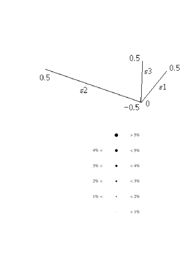
                 $\Delta R_{{}_{\rm MCE}}$

Figure 1: Percentage differences (11mouwyzaaadafahaj) between scalar-to-tensor ratios given by the GFM and those obtained from the WKB, ${\rm WKB*}$ and MCE.

5.3 Second slow-roll order MCE and WKB versus GFM

                  $|n_{\rm S\,\scriptscriptstyle{MCE}}-n_{\rm S\,\scriptscriptstyle{GFM}}|\times 100$                   $\Delta P_{\zeta\,\scriptscriptstyle{\rm MCE}}(k_{*})$

Figure 2: Left box: absolute difference between scalar spectral indeces $n_{\rm S}$ evaluated with the MCE and GFM (rescaled by a factor of $100$ for convenience). Note that relevant differences of order $0.05$ (shown as $5$) occur at the boundaries of the intervals considered for the $\epsilon_{i}$’s. Right box: percentage difference (11mouwyzaaadafahaj) for the amplitudes of scalar perturbations $P_{\zeta}$ at the pivot scale $k=k_{*}$ between the MCE and GFM. See Fig. 1 for the meaning of dot size.

$\Delta P_{\zeta\,\scriptscriptstyle{\rm MCE}}(k_{*})|_{\epsilon_{2}=-2\epsilon_{1}}$

Figure 3: Percentage difference (11mouwyzaaadafahaj) between the MCE and the GFM for $P_{\zeta}(k_{*})$ restricted on the hypersurface $\epsilon_{2}=-2\,\epsilon_{1}$, which corresponds to a scale-invariant spectrum to first order in the slow-roll expansion. The graph is given for $0<\epsilon_{1}<0.5$ and $-0.5<\epsilon_{3}<0.5$.

We shall now compare the slow-roll results obtained from the MCE and other methods of approximation previously employed [6] with those obtained using the GFM in the slow-roll expansion.We use the GFM just as a reference for the purpose of comparing the other methods among each other and of illustrating deviations from pure slow-roll results. For a given inflationary “observable” $Y$ evaluated with the method X, we denote the percentage difference with respect to its value given by the GFM as

$$\Delta Y_{{}_{\rm X}}\equiv 100\,\left|\frac{Y_{{}_{\rm X}}-Y_{{}_{\rm GFM}}}{Y_{{}_{\rm GFM}}}\right|\%\ ,$$ (11mouwyzaaadafahaj)

where ${\rm X}={\rm WKB}$ stands for the first WKB and second slow-roll orders [5], ${\rm X}={\rm WKB*}$ for the second WKB and second slow-roll orders [6] and, of course ${\rm X}={\rm MCE}$ for the result obtained in this paper. Note that for the case ${\rm X}={\rm WKB*}$ we shall set the three undetermined parameters $b_{\rm S}=b_{\rm T}=d_{\rm S}=2$ in order to minimize the difference with respect to the results of the GFM (see A and Ref. [6]).

In Fig. 1 we show, with dots of variable size, the percentage differences (11mouwyzaaadafahaj) for the scalar-to-tensor ratios $R$ at the pivot scale $k=k_{*}$ for $0<\epsilon_{1}<0.5$, $|\epsilon_{2}|$ and $|\epsilon_{3}|<0.5$. From the plots it appears that the level of accuracy of the MCE is comparable to that of the ${\rm WKB*}$ and both are (almost everywhere) more accurate than the WKB. However, the MCE achieves such a precision at leading order and is thus significantly more effective than the ${\rm WKB*}$. In Fig. 2 we show the difference in $n_{\rm S}$ and the relative difference in $P_{\zeta}(k_{*})$ between the MCE and GFM. In Fig. 3 we finally plot the relative difference in $P_{\zeta}(k_{*})$ for $\epsilon_{2}=-2\,\epsilon_{1}$ (the scale invariant case to first order in slow-roll parameters).

5.4 GFM and slow-roll approximation

Let us further compare our results with those obtained by the GFM. As we stated before, the most general result of the present work is given by the expressions for the power spectra (11moua) and (11moub) with the corrections (11mouc). In fact, the spectral indices and their runnings are the same as found with the standard WKB leading order [7, 6]. On the other hand, the main results of the GFM are the expressions for power spectra, spectral indices and runnings “$\ldots$ in the slow-roll expansion.” that is, for small HFF (see, e.g., Eqs. (41) and (43) in Ref. [3]). Here, and in some previous work [7, 8], we instead obtain results which hold for a general inflationary context, independently of the “slow-roll conditions”  or “slow-roll approximation” . The slow-roll case is just a possible application of our general expressions which can be evaluated for any model by simply specifying the scale factor. Our general, and non-local, expressions in fact take into account all the “history” of the HFF during inflation. For example, we note that the MCE at leading order reproduces the exact result for power-law inflation (see Sec. 5.1), whereas the GFM reproduces those to the next-to-leading order [3].

Chaotic inflation [27] is another example for which a Taylor approximation of the HFF (such as the one required by the GFM [3] or our Green’s function perturbative expansion in B) may lead to inaccurate results. We consider a quadratic potential

$$V(\phi)=\frac{1}{2}\,m^{2}\,\phi^{2}\ ,$$ (11mouwyzaaadafahak)

where $m$ is the mass of the inflaton $\phi$. In a spatially flat Robertson-Walker background, the potential energy dominates during the slow-rollover and the Friedman equation becomes

$$H^{2}=\frac{4\,\pi}{3\,m_{\rm Pl}^{2}}\,\left[\dot{\phi}^{2}+m^{2}\,\phi^{2}\right]\simeq\frac{4\,\pi\,m^{2}\,\phi^{2}}{3\,m_{\rm Pl}^{2}}\ .$$ (11mouwyzaaadafahal)

$H$
                                                    $t$

Figure 4: Numerical evolution of $H$ (solid line) and its analytic approximation (dashed line). The initial condition corresponds to $H_{i}\approx 8.2\,m$ (time in units of $1/m$) when the inflaton starts in the slow-roll regime with a value $4\,m_{\rm Pl}$.

The Hubble parameter evolves as

$$\dot{H}=-\frac{4\,\pi}{m_{\rm Pl}^{2}}\,\dot{\phi}^{2}\ .$$ (11mouwyzaaadafaham)

On using the equation of motion for the scalar field

$$\ddot{\phi}+3\,H\,\dot{\phi}+m^{2}\,\phi=0\ ,$$ (11mouwyzaaadafahan)

and neglecting the second derivative with respect to the cosmic time, we have $3\,H\,\dot{\phi}\simeq-\,m^{2}\,\phi$. Eq. (11mouwyzaaadafaham) then yields

$$\dot{H}\simeq-\frac{m^{2}}{3}\equiv\dot{H}_{0}\ ,$$ (11mouwyzaaadafahao)

which leads to a linearly decreasing Hubble parameter and, correspondingly, to an evolution for the scale factor which is not exponentially linear in time, i.e.

$$H(t)\simeq H_{0}+\dot{H}_{0}\,t\ ,$$ (11mouwyzaaadafahapa)

$$a(t)\simeq a(0)\,\exp\left(H_{0}\,t+\dot{H}_{0}\,\frac{t^{2}}{2}\right)\equiv a(0)\,\exp\left[N(t)\right]\ .$$ (11mouwyzaaadafahapb)

In Fig. 4 the analytic approximation (11mouwyzaaadafahapa) is shown to be very good on comparing with the exact (numerical) evolution. We are interested in the HFF in the slow-roll regime. From the definitions (11l) we then have

$$\epsilon_{1}(t)=-\frac{\dot{H}_{0}}{\left(H_{0}+\dot{H}_{0}\,t\right)^{2}}$$ (11mouwyzaaadafahapaqa)

$$\epsilon_{n}(t)=-\frac{2\,\dot{H}_{0}}{\left(H_{0}+\dot{H}_{0}\,t\right)^{2}}=2\,\epsilon_{1}(t)\ ,\quad n\geq 2\ ,$$ (11mouwyzaaadafahapaqb)

which we plot in Fig. 5.

$\epsilon_{i}$
                                                    $t$

Figure 5: HFF in the slow-roll regime: the dashed line is $\epsilon_{1}$ and the solid line is all the $\epsilon_{n}$’s with $n\geq 2$ (time in units of $1/m$).

Let us take the end of inflation at $t_{\rm end}\simeq 24/m$ (so that the analytic approximation (11mouwyzaaadafahapa), (11mouwyzaaadafahapb) is very good till the end), corresponding to $N_{\rm end}=125$ e-folds. We then consider the modes that leave the horizon 60 e-folds before the end of inflation and take that time ($t=t_{*}\simeq 8/m$ or $N_{*}=125-60=65$) as the starting point for a Taylor expansion to approximate the HFF ,

$$\epsilon_{i}\left(\Delta N\right)\simeq\epsilon_{i}+\epsilon_{i}\,\epsilon_{i+1}\,\Delta N+\frac{1}{2}\,\epsilon_{i}\,\left(\epsilon_{i+1}^{2}+\epsilon_{i+1}\,\epsilon_{i+2}\right)\,\Delta N^{2}\ ,$$ (11mouwyzaaadafahapaqar)

where the $\epsilon_{i}$’s in the r.h.s. are all evaluated at the time $t_{*}$ and $\Delta N=N-N_{*}$. The percentage error with respect to the analytic expressions (11mouwyzaaadafahapaqa) and (11mouwyzaaadafahapaqb) ,

$$\delta_{i}\equiv 100\,\left|\frac{\epsilon_{i}(t)-\epsilon_{i}\left(\Delta N\right)}{\epsilon_{i}(t)}\right|\%\ ,$$ (11mouwyzaaadafahapaqas)

with $\Delta N=N(t)-N_{*}$ is then plotted in Fig. 6 for $i=1$.

$\delta_{1}$
                                                    $t$

Figure 6: Percentage error for $\epsilon_{1}$ to first and second order in $\Delta N$ (dashed and solid line respectively; time in units of $1/m$).

It obviously becomes large rather quickly away from $t=t_{*}$ and we can immediately conclude that, had we used a Taylor expansion to approximate the HFF over the whole range of chaotic inflation ($-65<\Delta N<60$), we would have obtained large errors from the regions both near the beginning and the end of inflation.

In general, we expect that the Taylor expansion of the HFF will lead to a poor determination of the numerical coefficients (depending on $C$ in Eqs. (11mouwyzaaadafa) and (11mouwyzaaadafb)) in the second slow-roll order terms for those models in which the HFF vary significantly in time. In fact, we can calculate the integral of Eq. (21) in Ref. [3] with $\epsilon_{1}$ instead of the complete $g\left(\ln x\right)$ and $y_{0}(u)$ instead of $y(u)$. The percentage difference between this integral calculated using the Taylor expansion (11mouwyzaaadafahapaqar) with respect to the same integral calculated with $\epsilon_{1}$ in Eqs. (11mouwyzaaadafahapaqa) and (11mouwyzaaadafahapaqb) is $92\,\%$ and $88\,\%$ to first and second orders in $\Delta N$, respectively. The MCE method does not require such an expansion and does therefore not suffer from this restriction .

${\rm Log}(P_{Q})$
                                                    ${\rm Log}(k/k_{*})$

Figure 7: Spectrum of the Mukhanov variable $Q$ ($P_{Q}=k^{3}\,|Q_{k}|^{2}/(2\,\pi^{2})$) evaluated at the end of inflation for the chaotic model of Eq. (11mouwyzaaadafahak). The dots represent the numerical values and the solid line the analytic fit based on Eqs. (11mouwyzaaadafaha) and (11mouwyzaaadafahc) obtained by the second slow-roll order MCE approximation. The first order and GFM analytic results are not shown since they are almost indistinguishable from the MCE result plotted. $k_{*}$ crosses the Hubble radius at $\phi_{*}\simeq 3\,m_{\rm Pl}$ (the lines are normalized at $10^{2.25}\,k_{*}$).

We have also compared our analytic MCE results in Eqs. (11mouwyzaaadafaha) and (11mouwyzaaadafahc) with the numerical evaluation of the spectrum for scalar perturbations. In particular, we have evolved in cosmic time the modulus of the Mukhanov variable $Q$ (recalling that $P_{\zeta}=k^{3}\,|Q_{k}|^{2}/(2\,\pi^{2})$), which satisfies the associated non-linear Pinney equation [28]. The initial conditions for the numerical evolution are fixed for wave-lengths well within the Hubble radius and correspond to the adiabatic vacuum, i.e. $|Q_{k}(t_{i})|=1/(a(t_{i})\,\sqrt{k})$ and $|\dot{Q}_{k}|(t_{i})=-H(t_{i})\,|Q_{k}(t_{i})|$ [29]. The agreement of the analytic MCE approximation with the numerical results is good, as shown in Fig. 7.

5.5 Beyond slow-roll

The slow-roll approximation is quite accurate for a wide class of potentials. However, violations of the slow-roll approximation may occur during inflation, leading to interesting observational effects in the power spectra of cosmological perturbations. An archetypical model to study such violations is given by the potential

$$V(\phi)=V_{0}\,\left[1-\frac{2}{\pi}\,\arctan\left(N\,\frac{\phi}{m_{\rm Pl}}\right)\right]\ ,$$ (11mouwyzaaadafahapaqat)

introduced with $N=5$ in Ref. [30]. In Fig. 9 we show that the MCE result expanded to second slow-roll order provides a very good fit for the power spectrum of scalar perturbations even in situations where the slow-roll parameters are not very small (see Fig. 8). This example also shows that second slow-roll order results are much better than first order ones (analogous results were also obtained with the GFM in Ref. [26]).

$\epsilon_{i}$
                                                     $\phi/m_{\rm Pl}$

Figure 8: Evolution of $\epsilon_{i}$ with the value of the inflaton $\phi$ (in units of $m_{\rm Pl}$) in the arctan model of Eq. (11mouwyzaaadafahapaqat): $\epsilon_{1}$ (solid line), $\epsilon_{2}$ (long-dashed line) and $\dot{\epsilon}_{2}/H=\epsilon_{2}\,\epsilon_{3}$ (short-dashed line).

${\rm Log}(P_{Q})$
                                                     ${\rm Log}(k/k_{*})$

Figure 9: Spectrum of the Mukhanov variable $Q$ ($P_{Q}=k^{3}\,|Q_{k}|^{2}/(2\,\pi^{2})$) for the arctan model of Eq. (11mouwyzaaadafahapaqat). The dots represent the numerical values, the solid line the analytic results from Eqs. (11mouwyzaaadafaha) and (11mouwyzaaadafahc) obtained by the second slow-roll order MCE approximation and the dashed line those given by the first order slow-roll approximation. $k_{*}$ crosses the Hubble radius at $\phi_{*}\simeq-0.3\,m_{\rm Pl}$ (the lines are normalized at $10^{3/20}k_{*}$) and the spectrum is evaluated at $\simeq 55$ e-folds afterwards.

6 Conclusions

We have presented the application of the method of comparison equations to cosmological perturbations during inflation. By construction (i.e. by choosing a suitable comparison function), this approach leads to the exact solutions for inflationary models with constant horizon flow functions $\epsilon_{i}$’s (e.g. power-law inflation).

The main result is that, on using this approach to leading order, we were able to obtain the general expressions (11moua)-(11mouc) for the inflationary power spectra which are more accurate than those that any other method in the literature can produce at the corresponding order. In fact, the MCE leads to the correct asymptotic behaviours (in contrast with the standard slow-roll approximation [2]) and solves the difficulties in finding the amplitudes which were encountered with the WKB method [7].

Starting from the general results (11moua)-(11mouc), we have also computed the full analytic expressions for the inflationary power spectra to second slow-roll order in Eqs. (11mouwyzaaadafa) and (11mouwyzaaadafb) and found that the dependence on the horizon flow functions $\epsilon_{i}$’s is in agreement with that obtained by different schemes of approximation, such as the GFM [3] and the WKB approximation [5, 6]. Moreover, the results obtained with the MCE do not contain undetermined coefficients, in contrast with second slow-roll order results obtained with the WKB$*$ [6].

Let us conclude by remarking that, just like the WKB approach, the MCE does not require any particular constraints on the functions $\epsilon_{i}$’s and therefore has a wider range of applicability than any method which assumes them to be small. As an example, we have discussed in some detail the accuracy of the MCE for the massive chaotic and arctan inflationary models. We have shown that the MCE leads to accurate predictions even for a model which violates the slow-roll approximation during inflation.

Appendix A Impact of undetermined parameters in the WKB* approximation

To clarify the impact of the undetermined parameters $b_{\rm S}$, $b_{\rm T}$, and $d_{\rm S}=2$ on the results to second order in the HFF, the percentage differences between the numerical coefficients of some second order terms in the power spectra are displayed in Table 1 and of some of those in the scalar-to-tensor ratio in Table 2. All the entries are for $b_{\rm S}=b_{\rm T}=d_{\rm S}=2$, as is used in the main text, since other choices would give larger differences, as we explicitly show in Fig. 10 for the numerical coefficient in front of $\epsilon_{1}\,\epsilon_{2}$ in $P_{h}$ (since the behaviour is the same for all coefficients, we do not display other plots).

                                           $b_{\rm T}$

Figure 10: Percentage difference between the numerical coefficients of $\epsilon_{1}\,\epsilon_{2}$ in $P_{h}$ from ${\rm WKB*}$ and ${\rm GFM}$ as a function of $b_{\rm T}$. The difference vanishes for $b_{\rm T}\simeq 1.93$ ($\simeq 2$, the value used in the main text).

	$\epsilon_{1}^{2}$; $P_{\zeta}$, $P_{h}$	$\epsilon_{2}^{2}$; $P_{\zeta}$	$\epsilon_{1}\,\epsilon_{2}$; $P_{\zeta}(b_{\rm S}=2)$	$\epsilon_{1}\,\epsilon_{2}$; $P_{h}(b_{\rm T}=2)$
${\rm WKB}$	$2.3\%$	$3.0\%$	$353.3\%$	$37.2\%$
${\rm WKB*}$	$0.03\%$	$0.06\%$	$29.1\%$	$2.0\%$

Table 1: Percentage differences between the numerical coefficients of some second order terms in the power spectra given by ${\rm WKB}$ and ${\rm WKB*}$ with respect to those obtained by the GFM.

	$\epsilon_{2}\,\epsilon_{3}$; $(d_{\rm S}=2)$	$\epsilon_{1}\,\epsilon_{2}$; $(b_{\rm S}-b_{\rm T}=0)$	$\epsilon_{2}^{2}$
${\rm WKB}$	$56.7\%$	$1.5\%$	$117.3\%$
${\rm WKB*}$	$1.3\%$	$0.03\%$	$1.5\%$

Table 2: Percentage differences between the numerical coefficients of some second order terms in the scalar-to-tensor ratio given by ${\rm WKB}$ and ${\rm WKB*}$ with respect to those obtained from GFM. Note that the numerical coefficient of $\epsilon_{2}\,\epsilon_{3}$ in $R$ is the same as that in $P_{\zeta}$. Further, the coefficient of $\epsilon_{1}\,\epsilon_{2}$ does not depend on any undetermined parameters if $b_{\rm S}=b_{\rm T}$.

Appendix B Perturbative approximations

In this Section we present a possible method of obtaining the complete result to second order in the HFF. We start by noting that any given function $f=f(x)=f(\epsilon,x)$ can be written as the power series

$$\!\!\!\!\!\!\!f(\epsilon,x)=\sum_{n=0}^{\infty}\,\frac{x^{n}}{n!}\,\left(-\sum_{i}\,\frac{\hat{\epsilon}_{i}\,\hat{\epsilon}_{i+1}}{1-\hat{\epsilon}_{1}}\,\frac{\partial}{\partial\hat{\epsilon}_{i}}\right)^{n}f(\hat{\epsilon}_{i},x)\equiv\sum_{n=0}^{\infty}\,\frac{x^{n}}{n!}\,f_{n}(x)\ ,$$ (11mouwyzaaadafahapaqau)

where $\hat{\epsilon}_{i}=\epsilon_{i}(x_{*})$ are the HFF evaluated at the horizon crossing (i.e. at $x=x_{*}$) and $f(\hat{\epsilon}_{i},x)=f(\epsilon_{i}=\hat{\epsilon}_{i},x)$. On using Eqs. (11mouwyzaaadafahapaqau) to express both $\omega^{2}$ and $\chi$ in Eq. (1), we obtain

$$\!\!\!\!\!\!\!\!\!\!\!\!\!\!\!\!\!\!\!\!\chi_{0}(x)\,\sum_{n=1}^{\infty}\,\frac{x^{n}}{n!}\,\omega^{2}_{n}(x)+\left[\frac{{\mbox{${\rm d}$}}^{2}}{{\mbox{${\rm d}$}}x^{2}}+\sum_{m=0}^{\infty}\,\frac{x^{m}}{m!}\,\omega^{2}_{m}(x)\right]\,\sum_{n=1}^{\infty}\,\frac{x^{n}}{n!}\,\chi_{n}(x)=0\ ,$$ (11mouwyzaaadafahapaqav)

where we have used

$$\left[\frac{{\mbox{${\rm d}$}}^{2}}{{\mbox{${\rm d}$}}x^{2}}+\omega^{2}_{0}(x)\right]\,\chi_{0}(x)=0\ ,$$ (11mouwyzaaadafahapaqaw)

with $\omega^{2}_{0}(x)=\omega^{2}(\epsilon_{i}=\hat{\epsilon}_{i};x)$ and $\chi_{0}(x)$ is a linear combination (i.e. the MCE leading order solution) of Eq. (11mor) for $\Theta^{2}(x)=\omega^{2}_{0}(x)$ and $\sigma\to x$ in the argument of the Bessel functions. One may solve Eq. (11mouwyzaaadafahapaqav) for higher orders by introducing

$$\frac{x^{n}}{n!}\,\chi_{n}(x)\equiv g_{n}(x)\,\chi_{0}(x)\ ,$$ (11mouwyzaaadafahapaqax)

and using the standard formulae for second order differential equations with a source term, so that

$$\!\!\!\!\!\!\!\!\!\!\!\!\!\!\!\!\!\!\!\!\!\!\!\!\!\!\!\!\!\!\!\!\!\!\!\!\!\!\!\!g_{n}(x)=-\int_{\infty}^{x}\,\frac{\mbox{${\rm d}$}y}{\chi^{2}_{0}(y)}\,\int_{\infty}^{y}\,\mbox{${\rm d}$}z\,\chi^{2}_{0}(z)\left[\frac{z^{n}}{n!}\,\omega^{2}_{n}(z)+\sum_{m=1}^{n-1}\,g_{m}(z)\,\frac{z^{n-m}}{n-m}\,\omega^{2}_{n-m}(z)\right]\ .$$ (11mouwyzaaadafahapaqay)

The problem has therefore been reduced to computing $2\,n$ integrals.

The above formalism can be modified in order to provide an alternative way for calculating the power spectra, spectral indices and runnings to second order in the HFF. We start from Eq. (8) and (10) and the exact relations

$$\frac{z^{\prime\prime}_{\rm T}}{z_{\rm T}}=a^{2}\,H^{2}\,\left(2-\epsilon_{1}\right)$$

(11mouwyzaaadafahapaqaz)

$$\frac{z^{\prime\prime}_{\rm S}}{z_{\rm S}}=a^{2}\,H^{2}\,\left(2-\epsilon_{1}+\frac{3}{2}\,\epsilon_{2}-\frac{1}{2}\,\epsilon_{1}\,\epsilon_{2}+\frac{1}{4}\,\epsilon_{2}^{2}+\frac{1}{2}\,\epsilon_{2}\,\epsilon_{3}\right)\ .$$

With a redefinitions of the wave-function and variable

$$\psi={\rm e}^{-x/2}\,\mu\ ,\quad\quad\tilde{x}=\ln\left(-k\,\eta\right)$$ (11mouwyzaaadafahapaqba)

we obtain

$$\left[\frac{{\mbox{${\rm d}$}}^{2}}{{\mbox{${\rm d}$}}\tilde{x}^{2}}+\tilde{\omega}^{2}(\tilde{x})\right]\,\psi(\tilde{x})=0\ ,$$ (11mouwyzaaadafahapaqbb)

where

$$\tilde{\omega}^{2}_{\rm T}={\rm e}^{2\,\tilde{x}}-\frac{1}{4}-\eta^{2}a^{2}H^{2}\left(2-\epsilon_{1}\right)$$

(11mouwyzaaadafahapaqbc)

$$\!\!\!\!\!\!\!\!\!\!\!\!\!\!\!\!\!\!\!\!\!\tilde{\omega}^{2}_{\rm S}={\rm e}^{2\,\tilde{x}}-\frac{1}{4}-\eta^{2}a^{2}H^{2}\left(2-\epsilon_{1}+\frac{3}{2}\,\epsilon_{2}-\frac{1}{2}\,\epsilon_{1}\,\epsilon_{2}+\frac{1}{4}\,\epsilon_{2}^{2}+\frac{1}{2}\,\epsilon_{2}\,\epsilon_{3}\right)\ .$$

On now using the approximate relation

$$\eta\simeq-\frac{1}{a\,H}\,\left(1+\epsilon_{1}+\epsilon_{1}^{2}+\epsilon_{1}\,\epsilon_{2}\right)\ ,$$ (11mouwyzaaadafahapaqbd)

the frequencies become

$$\tilde{\omega}^{2}_{\rm T}\simeq{\rm e}^{2\,\tilde{x}}-\left(\frac{9}{4}+3\,\epsilon_{1}+4\,\epsilon_{1}^{2}+4\,\epsilon_{1}\epsilon_{2}\right)$$

(11mouwyzaaadafahapaqbe)

$$\!\!\!\!\!\!\!\!\!\!\!\!\!\!\!\!\!\!\!\!\tilde{\omega}^{2}_{\rm S}\simeq{\rm e}^{2\,\tilde{x}}-\left(\frac{9}{4}+3\,\epsilon_{1}+\frac{3}{2}\,\epsilon_{2}+4\,\epsilon_{1}^{2}+\frac{13}{2}\,\epsilon_{1}\epsilon_{2}+\frac{1}{4}\,\epsilon_{2}^{2}+\frac{1}{2}\,\epsilon_{2}\epsilon_{3}\right)\ ,$$

where we only keep the second order terms in the (still $\tilde{x}$-dependent) HFF. We can now expand linearly each HFF around the horizon crossing to obtain

$$\!\!\!\!\!\!\!\!\!\!\!\!\!\!\!\!\!\!\!\!\!\!\!\!\!\!\!\!\!\!\!\!\!\!\!\!\!\!\!\!\frac{{\mbox{${\rm d}$}}^{2}\,\psi_{\rm T}}{{\mbox{${\rm d}$}}\,\tilde{x}^{2}}\!+\!\left[{\rm e}^{2\,\tilde{x}}\!-\!\left(\frac{9}{4}+3\,\hat{\epsilon}_{1}+4\,\hat{\epsilon}_{1}^{2}+4\,\hat{\epsilon}_{1}\hat{\epsilon}_{2}\right)\right]\!\psi_{\rm T}=-3\,\hat{\epsilon}_{1}\,\hat{\epsilon}_{2}\,\tilde{x}\,\psi_{\rm T}$$

(11mouwyzaaadafahapaqbf)

$$\!\!\!\!\!\!\!\!\!\!\!\!\!\!\!\!\!\!\!\!\!\!\!\!\!\!\!\!\!\!\!\!\!\!\!\!\!\!\!\!\frac{{\mbox{${\rm d}$}}^{2}\,\psi_{\rm S}}{{\mbox{${\rm d}$}}\,\tilde{x}^{2}}\!+\!\left[{\rm e}^{2\,\tilde{x}}\!-\!\left(\frac{9}{4}+3\,\hat{\epsilon}_{1}+\frac{3}{2}\,\hat{\epsilon}_{2}+4\,\hat{\epsilon}_{1}^{2}+\frac{13}{2}\,\hat{\epsilon}_{1}\hat{\epsilon}_{2}+\frac{1}{4}\,\hat{\epsilon}_{2}^{2}+\frac{1}{2}\,\hat{\epsilon}_{2}\hat{\epsilon}_{3}\right)\right]\!\psi_{\rm S}$$

$$=-3\left(\hat{\epsilon}_{1}\,\hat{\epsilon}_{2}+\frac{1}{2}\,\hat{\epsilon}_{2}\,\hat{\epsilon}_{3}\right)\tilde{x}\,\psi_{\rm S}\ ,$$

which, beside the use of $\tilde{x}$ instead of $x$ and the appearance of $\tilde{\omega}$ instead of $\omega$, is equivalent to the expansion in Eq. (11mouwyzaaadafahapaqau) for $f=\tilde{\omega}^{2}$ and can be solved by means of a standard perturbative approach (such as in Ref. [3]). The method is close to GFM and gives the same results of Eq. (41) in Ref. [3] and Eq. (29) in Ref. [26] for the scalar and tensor power spectra, respectively.

Let us finally note that, for the GFM, the scalar spectral index and its running are calculated by taking the derivative of Eq. (41) in Ref. [3], i.e. the power spectra evaluated at $k=a\,H$, in terms of $\ln k$, while in our MCE (but also in the WKB approximation [5, 6]) the dependences in $\ln\left(k/k_{*}\right)$ are obtained explicitly (see, for example, Eqs. (11mouwyzaaadafa) and (11mouwyzaaadafb)).

References

References

- [1] Linde A D 1990 Particle physics and inflationary cosmology (Chur: Switzerland/Harwood) Liddle A R and Lyth D H 2000 Cosmological inflation and large-scale structure (Cambridge: England/Cambridge University Press)
- [2] Stewart E D and Lyth D H 1993 Phys. Lett. B 302 171
- [3] Stewart E D and Gong J-O 2001 P͡hys. Lett. B 510 1
- [4] Kosowsky A and Turner M S 1995 Phys. Rev. D 52 1739
- [5] Casadio R, Finelli F, Luzzi M and Venturi G 2005 Phys. Lett. B 625 1
- [6] Casadio R, Finelli F, Luzzi M and Venturi G 2005 Phys. Rev. D 72 103516
- [7] Martin J and Schwarz D J 2003 Phys. Rev. D 67 083512
- [8] Casadio R, Finelli F, Luzzi M and Venturi G 2005 Phys. Rev. D 71 043517
- [9] Miller S C and Good R H 1953 Phys. Rev. 91 174
- [10] Dingle R B 1956 Appl. Sci. Res. B 5 345
- [11] Berry M V and Mount K E 1972 Rep. Prog. Phys. 35 315
- [12] Langer R E 1937 Phys. Rev. 51 669
- [13] Kamenshchik A, Luzzi M and Venturi G 2005 Remarks on the method of comparison equations (generalized WKB method) and the generalized Ermakov-Pinney equation (Preprint math-ph/0506017)
- [14] Hecht C E and Mayer J E 1957 Phys. Rev. 106 1156
- [15] Moriguchi H 1959 J. Phys. Soc. Japan 14 1771
- [16] Pechukas P 1971 J. Chem. Phys. 54 3864
- [17] Mukhanov V F 1985 J. Exp. Theor. Phys. Lett. 41 493
- [18] Mukhanov V F 1988 Sov. Phys. JETP 67 1297
- [19] Grishchuk L P 1975 Sov. Phys. JETP 40 409
- [20] Starobinsky A A 1979 J. Exp. Theor. Phys. Lett. 30 682
- [21] Schwarz D J, Terrero-Escalante C A and Garcìa A A 2001 Phys. Lett. B 517 243
- [22] Abramowitz M and Stegun I 1965 Handbook of mathematical functions with formulas, graphs, and mathematical table (New York: Dover Publishing)
- [23] Lucchin F and Matarrese S 1985 Phys. Rev. D 32 1316
- [24] Lyth D H and Stewart E D 1992 Phys. Lett. B 274 168
- [25] Habib S, Heinen A, Heitmann K and Jungman G 2005 Phys. Rev. D 71 043518
- [26] Leach S M, Liddle A R, Martin J and Schwarz D J 2002 Phys. Rev. D 66 023515
- [27] Linde A D 1983 Phys. Lett. B 129 177
- [28] Bertoni C, Finelli F and Venturi G 1998 Phys. Lett. A 237 331
- [29] Finelli F, Marozzi G, Vacca G P, and Venturi G 2002 Phys. Rev. D 65 103521
- [30] Wang L M, Mukhanov V F and Steinhardt P J 1997 Phys. Lett. B 414 18