Gravitoelectromagnetic inflation from a 5D vacuum state: a new formalism

Abstract

We propose a novel formalism for inflation from a 5D vacuum state which could explain both, seeds of matter and magnetic fields in the early universe.

I Introduction

It is well known from observation that many spiral galaxies are endowed with coherent magnetic fields of $\mu G$ (micro Gauss) strength 1 ; 2 ; 3 ; 4 ; 5 ; 6 , having approximately the same energy density as the cosmic microwave background radiation (CMBR). For instance, the field strength of our galaxy is $B\simeq 3\times 10^{-6}\ G$, similar to that detected in high redshift galaxies uno and damped Lyman alpha clouds dos . There is also evidence for larger-scale magnetic fields of similar strength within clusters6' , which have been recently reviewed by Giovanninitres and by Carilli and Taylorcuatro . These fields can play an important role in various astrophysical processes, such as the confinement of cosmic rays and the transfer of angular momentum away from protostellar clouds, which leads to collapse and formation of stars. The presence of magnetic fields at even larger scales has also been claimed7 . These fields influence the formation process of large-scale structure8 ; 9 . Recentlyocho the possible existence, strength and structure of magnetic fields in the intergalactic plane, within the Local Supercluster, has been scrutinized. The local supercluster is centered approximately at the VIRGO cluster. A statistically significant Faraday screening acting on the radio-waves coming from the most distant sources has been found. This analysis supports the existence of a regular magnetic field of $0.3\ \mu G$ in the local supercluster. More recent discussions of possible observational consequences on cosmological magnetic fields that include the effects on the CMB anisotropy were made inkoso . Several mechanisms have been proposed to explain the origin of the seed field. It has been suggested that a primordial field may be produced during the inflationary period if conformal invariance is brokencinco ; seis . In string-inspired models, the coupling between the electromagnetic field and the dilaton breaks conformal invariance and may produce the seed fieldsiete .

Inflation has nowadays become a standard ingredient for the description of the early universe. In fact, it solves some of the problems of the standard big-bang scenario and also makes predictions about CMBR anisotropies which are being measured with higher and higher precision. The first model of inflation was proposed by Starobinsky in 1979star . A much simpler inflationary model with a clear motivation was developed by Guth in the 80’sguth . However, the universe after inflation in this scenario becomes very inhomogeneous. These problems were sorted out by Linde in 1983 with the introduction of chaotic inflationlinde . Inflation offers the hope of furnishing a mechanism for kinematically and dynamically producing the seed of cosmic magnetic fields. It provides the kinematic means for producing long-wavelength effects in the very early universe by the amplification of short-wavelength modes of the inflaton field. This also could have happened with modes of an electromagnetic field. Since an electromagnetic wave with $\lambda_{phys}\geq H^{-1}_{0}$ has the appearance of static $\vec{E}$ and $\vec{B}$ fields, very long wavelength photons ($\lambda_{phys}\gg H^{-1}_{0}$) could lead to large-scale magnetic fields.

In this work we shall study a cosmological formalism for inflation from a 5D vacuum state, where the effective 4D matter, electromagnetic and vacuum effects are induced geometrically. The formalism is aimed to explain both, seeds of matter and magnetic fields in the early universe.

II 5D Formalism

We consider the 5D canonical metriclb

$$dS^{2}=\psi^{2}dN^{2}-\psi^{2}e^{2N}dr^{2}-d\psi^{2},$$ (1)

where $dr^{2}=dx^{2}+dy^{2}+dz^{2}$. In this line element the coordinates $(N,r)$ are dimensionless and the fifth one $\psi$ has spatial units. This metric describes a 5D flat manifold in apparent vacuum $G_{AB}=0$ and satisfies $R^{A}\,_{BCD}=0$, i. e., it’s flat. To describe an electromagnetic field and neutral matter on this background, we consider the action

$$I=\int d^{4}xd\psi\sqrt{\left|\frac{{}^{(5)}g}{{}^{(5)}g_{0}}\right|}\left[\frac{{}^{(5)}R}{16\pi{\rm G}}+^{(5)}{\cal L}(A_{B},A_{C;B})\right]$$ (2)

for a vector potencial with components $A_{B}=(A_{\mu},\varphi)$, which are minimally coupled to gravity. Here, ${}^{(5)}R$ is the 5D Ricci scalar, which is zero for the metric (1).

We propose a 5D lagrangian density in (2)

$$^{(5)}{\cal L}(A_{B},A_{B;C})=-\frac{1}{4}Q_{BC}Q^{BC}$$ (3)

where we define the tensor field $Q_{BC}=F_{BC}+\gamma g_{BC}\left(A^{D}\,_{;D}\right)$, with $\gamma=\sqrt{\frac{2\lambda}{5}}$ and $F_{BC}=A_{C;B}-A_{B;C}=-F_{CB}$, being $(;)$ the covariant derivative. The lagrangian density (3) can also be expressed as

$$^{(5)}{\cal L}(A_{B},A_{B;C})=-\frac{1}{4}F_{BC}F^{BC}-\frac{\lambda}{2}\left(A^{D}\,_{;D}\right)^{2},$$ (4)

where the last term is a “gauge-fixing” term. The 5D-dynamics field equations in a Lagrange formalism leads to

$$A^{B}\,_{;D}\,{}^{;D}-(1-\lambda)A^{C}\,_{;C}\,{}^{;B}=0.$$ (5)

Working in the Feynman gauge $(\lambda=1)$, the equation (5) yields

$$\frac{1}{\sqrt{\left|{}^{(5)}g\right|}}\frac{\partial}{\partial x^{C}}\left[\sqrt{\left|{}^{(5)}g\right|}\,g^{DC}A^{B}\,_{,D}\right]=0,$$ (6)

where $A^{B}=(A^{\mu},-\varphi)$. Equation (6) is a massless Klein-Gordon-like equation for $A^{B}$ and represents the analogous of the Maxwell’s equations in a 5D manifold in an apparent vacuum. The commutators for $A^{C}$ and $\bar{\Pi}^{B}=\frac{\partial{\cal L}}{\partial(A_{B,N})}=F^{BN}-g^{BN}A^{C}\,_{;C}$ are given by

$$\left[A^{C}(N,\vec{r},\psi),\bar{\Pi}^{B}(N,\vec{r^{\prime}},\psi^{\prime})\right] = ig^{CB}g^{NN}\left|\frac{{}^{(5)}g_{0}}{{}^{(5)}g}\right|\delta^{(3)}\left(\vec{r}-\vec{r^{\prime}}\right)\delta\left(\psi-\psi^{\prime}\right),$$ (7)

$$\left[A_{C}(N,\vec{r},\psi),A_{B}(N,\vec{r^{\prime}},\psi^{\prime})\right] = \left[\bar{\Pi}_{C}(N,\vec{r},\psi),\bar{\Pi}_{B}(N,\vec{r^{\prime}},\psi^{\prime})\right]=0.$$ (8)

Here $\bar{\Pi}^{N}=-g^{NN}\left(A^{C}\,_{;C}\right)$ and $\left|\frac{{}^{(5)}g_{0}}{{}^{(5)}g}\right|$ is the inverse of the normalized volume of the manifold (1). From the equation (8), we obtain

$$\left[A_{C}(N,\vec{r},\psi),A_{B;N}(N,\vec{r^{\prime}},\psi^{\prime})\right]=-i\ g_{BC}\left|\frac{{}^{(5)}g_{0}}{{}^{(5)}g}\right|\delta^{(3)}\left(\vec{r}-\vec{r^{\prime}}\right)\ \delta\left(\psi-\psi^{\prime}\right).$$ (9)

Using equations (1) and (6), the equation of motion for the electromagnetic 4-vector potential $A^{\mu}$, is given by

$$\stackrel{{\scriptstyle\star\star}}{{A^{\mu}}}+3\stackrel{{\scriptstyle\star}}{{A^{\mu}}}-e^{-2N}\nabla_{r}^{2}A^{\mu}-\left[4\psi\frac{\partial A^{\mu}}{\partial\psi}+\psi^{2}\frac{\partial^{2}A^{\mu}}{\partial\psi^{2}}\right]=0,$$ (10)

where the overstar denotes the derivative with respect to N. Similarly for $\varphi$ we have

$$\stackrel{{\scriptstyle\star\star}}{{\varphi}}+3\stackrel{{\scriptstyle\star}}{{\varphi}}-e^{-2N}\nabla_{r}^{2}\varphi-\left[4\psi\frac{\partial\varphi}{\partial\psi}+\psi^{2}\frac{\partial^{2}\varphi}{\partial\psi^{2}}\right]=0.$$ (11)

Furthermore, using (7) the commutator between $\varphi$ and $\stackrel{{\scriptstyle\star}}{{\varphi}}$ becomes

$$\left[\varphi(N,\vec{r},\psi),\stackrel{{\scriptstyle\star}}{{\varphi}}(N,\vec{r^{\prime}},\psi^{\prime})\right]=i\left|\frac{{}^{(5)}g_{0}}{{}^{(5)}g}\right|\delta^{(3)}\left(\vec{r}-\vec{r^{\prime}}\right)\delta\left(\psi-\psi^{\prime}\right).$$ (12)

which is the same expression that whole obtained in MB1 .

II.1 The 4D Electromagnetic Field embedded in 5D.

Transforming $A^{\mu}$ according to $A^{\mu}(N,\vec{r},\psi)=e^{-3N/2}\left(\frac{\psi_{0}}{\psi}\right)^{2}\bar{A}^{\mu}(N,\vec{r},\psi)$, and from the equation (10), we have

$$\stackrel{{\scriptstyle\star\star}}{{\bar{A}^{\mu}}}-e^{-2N}\nabla_{r}^{2}\bar{A}^{\mu}-\psi^{2}\frac{\partial^{2}\bar{A}^{\mu}}{\partial\psi^{2}}-\frac{1}{4}\bar{A}^{\mu}=0,$$ (13)

so that the commutator between $\stackrel{{\scriptstyle\star}}{{\bar{A}^{\mu}}}$ and $\bar{A}^{\nu}$ becomes

$$\left[\stackrel{{\scriptstyle\star}}{{\bar{A}^{\mu}}}(N,\vec{r},\psi),\bar{A}^{\nu}(N,\vec{r^{\prime}},\psi^{\prime})\right]=ig^{\mu\nu}\delta^{(3)}\left(\vec{r}-\vec{r^{\prime}}\right)\delta\left(\psi-\psi^{\prime}\right).$$ (14)

The redefined electromagnetic field $\bar{A}^{\mu}$ can be expressed in terms of a Fourier expansion

$$\bar{A}^{\mu}(N,\vec{r},\psi)=\frac{1}{(2\pi)^{3/2}}\int d^{3}k_{r}\int dk_{\psi}\sum_{\alpha=0}^{3}\epsilon_{(\alpha)}^{\mu}\left[a_{k_{r}k_{\psi}}^{(\alpha)}e^{i\vec{k}_{r}\cdot\vec{r}}\zeta_{k_{r}k_{\psi}}(N,\psi)+a_{k_{r}k_{\psi}}^{(\alpha)\,\dagger}e^{-i\vec{k}_{r}\cdot\vec{r}}\zeta_{k_{r}k_{\psi}}^{*}(N,\psi)\right]$$ (15)

where the creation and annihilation operators ($a_{k_{r}k_{\psi}}^{(\alpha)\dagger}$, $a_{k_{r}k_{\psi}}^{(\alpha)}$) comply

$$\left[a_{k_{r}k_{\psi}}^{(\alpha)},a_{k^{\prime}_{r}k^{\prime}_{\psi}}^{(\alpha^{\prime})\,\dagger}\right] = -g^{\alpha\alpha^{\prime}}\delta^{(3)}\left(\vec{k}_{r}-\vec{k^{\prime}}_{r}\right)\delta\left(k_{\psi}-k^{\prime}_{\psi}\right),$$ (16)

$$\left[a_{k_{r}k_{\psi}}^{(\alpha)},a_{k^{\prime}_{r}k^{\prime}_{\psi}}^{(\alpha^{\prime})}\right] = \left[a_{k_{r}k_{\psi}}^{(\alpha)\,\dagger},a_{k^{\prime}_{r}k^{\prime}_{\psi}}^{(\alpha^{\prime})\,\dagger}\right]=0,$$ (17)

and the four polarisation 4-vectors $\epsilon^{\mu}_{(\alpha)}$ satisfy $\epsilon_{(\alpha)}\cdot\epsilon_{(\alpha^{\prime})}=g_{\alpha\alpha^{\prime}}$. Using the expansion (15), into the equation (13), we find

$$\frac{\partial^{2}}{\partial N^{2}}\zeta_{k_{r}k_{\psi}}+\left[e^{-2N}k_{r}^{2}-\frac{1}{4}\right]\zeta_{k_{r}k_{\psi}}-\psi^{2}\frac{\partial^{2}}{\partial\psi^{2}}\zeta_{k_{r}k_{\psi}}=0,$$ (18)

which is the dynamical equation for the modes $\zeta_{k_{r}k_{\psi}}$ of $\bar{A}^{\mu}$. We propose that $\zeta_{k_{r}k_{\psi}}$ can be decomposed as $\zeta_{k_{r}k_{\psi}}(N,\psi)=\zeta_{(1)}(N)\zeta_{(2)}(\psi)$, where for simplicity, we have suppressed the underscripts $k_{r}k_{\psi}$ in the notation. Thus, equation (18) can be equivalently expressed by the system of equations

$$\psi^{2}\frac{d^{2}}{d\psi^{2}}\zeta_{(2)}-\kappa^{2}\zeta_{(2)} = 0,$$ (19)

$$\frac{d^{2}}{dN^{2}}\zeta_{(1)}+\left[k_{r}^{2}e^{-2N}-\left(\kappa^{2}+\frac{1}{4}\right)\right]\zeta_{(1)} = 0,$$ (20)

where $\kappa$ is a dimensionless separation constant given by $\kappa^{2}=\psi^{2}k^{2}_{\psi}$, being $k_{\psi}$ the wavenumber corresponding to the fifth coordinate. The general solution for the system (19,20) is given by

$$\zeta_{k_{r}k_{\psi}}(N,\psi)=C_{1}{\cal H}_{\nu_{1}}^{(1)}[x(N)]+C_{2}{\cal H}_{\nu_{1}}^{(2)}[x(N)],$$ (21)

where $\nu_{1}={\sqrt{4k^{2}_{\psi}\psi^{2}+1}\over 2}$ is a dimensionless constant and $x(N)=k_{r}e^{-N}$. In this equation ${\cal H}_{\nu_{1}}^{(1)}$ and ${\cal H}_{\nu_{1}}^{(2)}$ are the first and second kind Hankel functions. The normalization condition for $\zeta_{k_{r}k_{\psi}}(N,\psi)$ becomes

$$\zeta_{k_{r}k_{\psi}}\stackrel{{\scriptstyle\star}}{{\zeta}}_{k_{r}k_{\psi}}^{\,*}-\stackrel{{\scriptstyle\star}}{{\zeta}}_{k_{r}k_{\psi}}\zeta_{k_{r}k_{\psi}}^{*}=i.$$ (22)

Therefore, considering the Bunch-Davies vacuum, $C_{1}=0$ and $C_{2}=i\sqrt{\pi}/2$, we obtain

$$\zeta_{k_{r}k_{\psi}}(N,\psi)=i\frac{\sqrt{\pi}}{2}{\cal H}_{\nu_{1}}^{(2)}[x(N)],$$ (23)

which gives the normalized modes corresponding to the electromagnetic field embedded in a 5D aparent vacuum.

III Effective 4D dynamics.

Considering the coordinate transformations

$$t=\psi_{0}N,\quad R=r\psi_{0},\quad\psi=\psi,$$ (24)

equation (1) takes the form

$$dS^{2}=\left(\frac{\psi}{\psi_{0}}\right)^{2}\left[dt^{2}-e^{2t/\psi_{0}}dR^{2}\right]-d\psi^{2},$$ (25)

which is the Ponce Leon metric that describes a 3D spatially flat, isotropic and homogeneous extension to 5D of a Friedmann Robertson Walker (FRW) line element in a de Sitter expansion. Here $t$ is the cosmic time and $dR^{2}=dX^{2}+dY^{2}+dZ^{2}$. Now, we can take the foliation $\psi=\psi_{0}$ in (25), such that we obtain the effective 4D metric

$$dS^{2}\rightarrow ds^{2}=dt^{2}-e^{2H_{0}t}dR^{2},$$ (26)

which describes a 3D spatially flat, isotropic and homogeneous de Sitter expanding Universe with a constant Hubble parameter $H_{0}=1/\psi_{0}$ and a 4D scalar curvature ${}^{(4)}{\cal R}=12H^{2}_{0}$.

Equation (10) with the transformation (24) and the foliation $\psi=\psi_{0}=H_{0}^{-1}$, provides the effective equation of motion for $A^{\mu}(t,\vec{R},\psi=\psi_{0})\equiv A^{\mu}(t,\vec{R})$

$$\ddot{A}^{\mu}+3H_{0}\dot{A}^{\mu}-e^{-2H_{0}t}\nabla_{R}^{2}A^{\mu}-H_{0}^{2}\left.\left[4\psi\frac{\partial A^{\mu}}{\partial\psi}+\psi^{2}\frac{\partial^{2}A^{\mu}}{\partial\psi^{2}}\right]\right|_{\psi=H_{0}^{-1}}=0,$$ (27)

where $A^{\mu}$ is the effective 4D electromagnetic field induced onto the hypersurface $\psi=H_{0}^{-1}$. Note that the last term between brackets acts as an induced electromagnetic potential derived with respect $A^{\mu}$. This term is the analogous to $V^{\prime}(\varphi)$ in the case of an inflationary scalar field as used in madbe , and in our case the dynamics of the component $A^{4}\equiv-\varphi$ is described by

$$\ddot{\varphi}+3H_{0}\dot{\varphi}-e^{-2H_{0}t}\nabla_{R}^{2}\varphi-H_{0}^{2}\left.\left[4\psi\frac{\partial\varphi}{\partial\psi}+\psi^{2}\frac{\partial^{2}\varphi}{\partial\psi^{2}}\right]\right|_{\psi=H_{0}^{-1}}=0.$$ (28)

On the other hand, transforming $A^{\mu}$ as $A^{\mu}(t,\vec{R})=e^{-\frac{3}{2}H_{0}t}{\cal A}^{\mu}(t,\vec{R})$, the equation (27) takes the form

$$\ddot{{\cal A}}^{\mu}-e^{-2H_{0}t}\nabla_{R}^{2}{\cal A}^{\mu}-\left(\frac{9}{4}H_{0}^{2}+\alpha\right){\cal A}^{\mu}=0,$$ (29)

where $\alpha=k_{\psi_{0}}^{2}-2H_{0}^{2}$ is a constant parameter. Expressing ${\cal A}^{\mu}(t,\vec{R})$ as a Fourier expansion

$${\cal A}^{\mu}(t,\vec{R})=\frac{1}{(2\pi)^{3/2}}\int d^{3}k_{R}\int d_{k_{\psi}}\sum_{\gamma=0}^{3}\epsilon_{(\gamma)}^{\mu}\left[a_{k_{R}}^{\gamma}e^{i\vec{k}_{R}\cdot\vec{R}}Q_{k_{R}}(t)+cc\right]\delta(k_{\psi}-k_{\psi_{0}}),$$ (30)

where $k_{\psi_{0}}$ is a constant. The equation of motion for the effective 4D electromagnetic modes $Q_{k_{R}}(t)$, becomes

$$\ddot{Q}_{k_{R}}+\left[k_{R}^{2}e^{-2H_{0}t}-\left(\frac{9}{4}H_{0}^{2}+\alpha\right)\right]Q_{k_{R}}=0,$$ (31)

whose general solution is

$$Q_{k_{R}}(t)=F_{1}{\cal H}_{\nu}^{(1)}[y(t)]+F_{2}{\cal H}_{\nu}^{(2)}[y(t)],$$ (32)

where $y(t)=\frac{k_{R}}{H_{0}}e^{-H_{0}t}$ and $\nu=\frac{1}{2H_{0}}\sqrt{9H_{0}^{2}+\alpha}$.

The corresponding normalization condition for the modes $Q_{k_{R}}(t)$ becomes

$$Q_{k_{R}}\dot{Q}_{k_{R}}^{*}-\dot{Q}_{k_{R}}Q_{k_{R}}^{*}=i.$$ (33)

Note that $H_{0}$ remains constant in a de Sitter expansion. Therefore, taking into account the Bunch-Davies vacuum condition, we consider $F_{1}=0$ and $F_{2}=i\sqrt{{\pi\over 4H_{0}}}$. Hence the normalized solution of (31) is

$$Q_{k_{R}}(t)=i\sqrt{\frac{\pi}{4H_{0}}}{\cal H}_{\nu}^{(2)}[y(t)].$$ (34)

which describes the normalized effective 4D-modes corresponding to the effective 4D electromagnetic field $A^{\mu}$.

III.1 Classicality conditions of $A_{\mu}$

It is very important to see that all the modes $Q_{k_{R}}(t)$ on the infrared (IR) sector are real. If we write these modes as a complex function with components $u_{k_{R}}(t)$ and $v_{k_{R}}(t)$: $Q_{k_{R}}(t)=u_{k_{R}}(t)+iv_{k_{R}}(t)$, the condition for the modes to be real is

$$\alpha_{k_{R}}(t)=\left|\frac{v_{k_{R}}(t)}{u_{k_{R}}(t)}\right|\ll 1.$$ (35)

Hence, the condition for the field $A_{\mu}$ to be classical on the IR sector during inflation, becomes

$$\frac{1}{M(t)}\sum^{k_{r}\simeq\vartheta k_{H}(t)}_{k_{R}=0}\alpha_{k_{R}}(t)\ll 1,$$ (36)

where $M(t)$ is the time-dependent number of degrees of freedom (which increases with time during inflation) in the IR ($k_{R}\ll k_{H}$) sector. The coarse-graining field

$$\left.{\cal A}_{\mu}\right|_{IR}=\frac{1}{(2\pi)^{3/2}}{\Large\int}d^{3}k_{R}\Theta(\epsilon k_{H}-k_{R})\sum^{3}_{\gamma=0}\epsilon^{\mu}_{(\gamma)}\left[a^{\gamma}_{k_{R}k_{\psi_{0}}}e^{i\vec{k}_{R}.\vec{R}}Q_{k_{R}}(t)+c.c.\right],$$ (37)

(here $\Theta$ denotes the Heaviside function), takes into account only the modes with $10^{3}\ll\vartheta^{-1}<k_{H}/k_{R}$ that can be considered as classical because

$$\left[\left.{\cal A}_{\mu}\right|_{IR},\left.\dot{\cal A}_{\mu}\right|_{IR}\right]\simeq 0,$$ (38)

which in turn implies that the fluctuations of $\left.A_{\mu}\right|_{IR}$ can be treated as classical in the electromagnetic field as well.

III.2 Electromagnetic fields during inflation

Previous results allow us to calculate the effective 4D super Hubble squared fluctuations of the electromagnetic field $<0|A^{\mu}A_{\mu}|0>=\left<A^{2}\right>$, which are given by

$$\left.\left<A^{2}\right>\right|_{IR}=\frac{2e^{-3H_{0}t}}{\pi^{2}}\int_{0}^{\vartheta k_{H}}\frac{dk_{R}}{k_{R}}k_{R}^{3}Q_{k_{R}}Q_{k_{R}}^{*},$$ (39)

where $\vartheta=\frac{k_{max}^{(IR)}}{k_{p}}\ll 1$ is a dimensionless parameter. Here, $k_{max}^{(IR)}=k_{H}(t_{i})=H_{0}e^{H_{0}t_{i}}$ is the wavenumber related to the Hubble radius at $t_{i}$ (the time when the horizon enters) and $k_{p}$ is the Planckian wavenumber. In fact we choose $k_{p}$ as a cut-off scale of all the spectrum.

To obtain $\left.\left<A^{2}\right>\right|_{IR}$, we must consider the small argument limit for ${\cal H}_{\nu}^{(2)}[y]\simeq\frac{\left(\frac{y}{2}\right)^{\nu}}{\Gamma(1+\nu)}-\frac{i}{\pi}\Gamma(\nu)\left(\frac{y}{2}\right)^{-\nu}$. From the condition (35) we obtain that each $k_{R}$-mode becomes classical for times

$$t\gg\frac{1}{2\nu H_{0}}\ {\rm ln}\left[\frac{\Gamma(\nu)}{\Gamma(1+\nu)2^{2\nu}}\left(\frac{k_{R}}{H_{0}}\right)^{2\nu}\right],$$ (40)

which for a de Sitter expansion takes the form $\frac{k_{R}}{H_{0}}\ll e^{N_{e}}$ and $N_{e}$ is the number of e-folds at the end of inflation. In order for inflation to solve the horizon/flatness problem, $N_{e}\geq 60$ is required. Note that in this case when $k_{\psi_{0}}^{2}\simeq 2H_{0}^{2}$, the constant parameter $|\alpha|/H^{2}_{0}\ll 1$ and thus $\nu\simeq 3/2$. Hence we can use ${\cal H}_{\nu}^{(2)}[y]\simeq-\frac{i}{\pi}\Gamma(\nu)\left(\frac{y}{2}\right)^{-\nu}$ on the IR sector to obtain

$$\left.\left<A^{2}\right>\right|_{IR}\simeq\frac{2^{2\nu-1}}{\pi^{3}}H_{0}^{2\nu-1}\Gamma^{2}(\nu)e^{-(3-2\nu)H_{0}t}\int_{0}^{\vartheta k_{H}}\frac{dk_{R}}{k_{R}}k_{R}^{3-2\nu}.$$ (41)

Note that when $\alpha=0$, $\nu=3/2$ and thus the spectrum ${\cal P}(k_{R})\sim k_{R}^{3-2\nu}$ is scale invariant. Performing the remaining integration, (41) becomes

$$\left.\left<A^{2}\right>\right|_{IR}\simeq\frac{2^{2\nu-1}}{\pi^{3}}\frac{\Gamma^{2}(\nu)}{(3-2\nu)}H_{0}^{2}\vartheta^{3-2\nu},$$ (42)

which is similar to the corresponding $\left.\left<\varphi^{2}\right>\right|_{IR}$. We must note that $\left<A^{2}\right>$ has constant value in the infrared sector, which means that the amplitude of the corresponding photons is constant. This result can be interpreted as a classical large-scale electromagnetic potential generated when a de Sitter inflationary process ends, which is responsible for a large-scale seed magnetic field.

IV Induced seed magnetic field.

In this section we estimate the seed magnetic field induced from the electromagnetic potential whose dynamics was studied in the previous section. For this purpose we consider the 3D spatial components of $\vec{A}=A^{i}\hat{e}_{i}$ ($\hat{e}_{i}$ are the 3D spatial basis vectors), which in view of (27) and (29) satisfy

$$\ddot{A}^{i}+3H_{0}\dot{A}^{i}-e^{-2H_{0}t}\nabla_{R}^{2}A^{i}-\alpha A^{i}=0.$$ (43)

We consider the physical components of $\vec{A}$ and $\vec{B}$ measured in a comoving frame. Hence, the orthonormal basis components associated with the observers in this frame are given by

$$e_{(t)}=\frac{\partial}{\partial t},\qquad e_{(\bar{R})}=e^{-H_{0}t}\frac{\partial}{\partial\bar{R}},\qquad e_{(\theta)}=e^{-H_{0}t}\frac{1}{\bar{R}}\frac{\partial}{\partial\theta},\qquad e_{(\phi)}=e^{-H_{0}t}\frac{1}{\bar{R}\ {\rm sin}\theta}\frac{\partial}{\partial\phi},$$ (44)

where the spatial part of (26) has been rewritten as $dR^{2}=d\bar{R}^{2}+\bar{R}^{2}(d\theta^{2}+{\rm sin}^{2}\theta d\phi^{2})$.

On the other hand, we know that from (10) through the transformations (24) we can obtain the standard Maxwell’s equations with sources, where such sources have a geometrical origin. The Maxwell’s equations without sources can be obtained from these (see Jackson ). Therefore, using $\vec{\nabla}_{R}\cdot\vec{B}_{com}=0$ and $\vec{B}_{com}=\vec{\nabla}_{R}\times\vec{A}_{com}$, equation (43) becomes

$$\ddot{B}^{i}_{com}+H_{0}\dot{B}^{i}_{com}-e^{-2H_{0}t}\nabla_{R}^{2}B^{i}_{com}-(\alpha+2H_{0}^{2})B^{i}_{com}=0.$$ (45)

This expression describes the dynamics of the comoving components of the seed magnetic field. As in the case of $A^{\mu}$, we can express these components as a Fourier expansion

$$B^{i}_{com}(t,\vec{R})=\frac{e^{-\frac{1}{2}H_{0}t}}{(2\pi)^{3/2}}\int d^{3}k_{R}\sum_{l=1}^{3}\epsilon_{(l)}^{i}(k_{R})\left[b_{k_{R}}^{(l)}e^{i\vec{k}_{R}\cdot\vec{R}}G_{k_{R}}(t)+b_{k_{R}}^{(l)\,\dagger}e^{-i\vec{k}_{R}\cdot\vec{R}}G_{k_{R}}^{*}(t)\right],$$ (46)

where $b_{k_{R}}^{(l)\,\dagger}$ and $b_{k_{R}}^{(l)}$ are the creation and annihilation operators and $\epsilon_{(l)}^{i}(k_{R})$ are the 3-polarisation vectors which satisfy $\epsilon_{(i)}\cdot\epsilon_{(j)}=g_{ij}$. Therefore, the equation of motion for $G_{k_{R}}(t)$ obtained from (45), acquires the form

$$\ddot{G}_{k_{R}}+\left[k_{R}^{2}e^{-2H_{0}t}-\left(\frac{9}{4}H_{0}^{2}+\alpha\right)\right]G_{k_{R}}=0,$$ (47)

and has for solution

$$G_{k_{R}}(t)=L_{1}{\cal H}_{\nu}^{(1)}[w(t)]+L_{2}{\cal H}_{\nu}^{(2)}[w(t)],$$ (48)

where $\nu=\frac{1}{2H_{0}}\sqrt{9H_{0}^{2}+4\alpha}$, $w(t)=\frac{k_{R}}{H_{0}}e^{-H_{0}t}$ and $L_{1}$, $L_{2}$ are integration constants. The corresponding normalization condition for those seed magnetic modes is

$$G_{k_{R}}\dot{G}_{k_{R}}^{*}-\dot{G}_{k_{R}}G_{k_{R}}^{*}=i/a^{2}_{0},$$ (49)

being $a_{0}=H^{-1}_{0}$ the scale factor of the universe when inflation begins.

The normalized solution of (47) is

$$G_{k_{R}}(t)=i\sqrt{\frac{\pi H_{0}}{4}}{\cal H}_{\nu}^{(2)}[w(t)].$$ (50)

Now, the super Hubble squared $B$ fluctuations of the seed magnetic field $\left<B^{2}_{com}\right>$ in the Feynman gauge are given by

$$\left.\left<B^{2}_{com}\right>\right|_{IR}=\frac{3e^{-H_{0}t}}{2\pi^{2}}\int_{0}^{\vartheta k_{H}}\frac{dk_{R}}{k_{R}}\,k_{R}^{3}G_{k_{R}}(t)G_{k_{R}}^{*}(t)=\int_{0}^{\vartheta k_{H}}\frac{dk_{R}}{k_{R}}\ {\cal P}(k_{R}),$$ (51)

where $\vartheta=\frac{k_{max}^{(IR)}}{k_{p}}\ll 1$ is a dimensionless parameter. We are choosing $k_{p}$ as a cut-off scale of the whole spectrum. The power spectrum ${\cal P}(k_{R})$ on cosmological scales is

$${\cal P}(k_{R})=\frac{3}{8\pi^{3}}2^{2\nu}\Gamma^{2}(\nu)H_{0}^{1+2\nu}e^{-(1-2\nu)H_{0}t}k_{R}^{3-2\nu}.$$ (52)

Considering the case $k_{\psi_{0}}^{2}\simeq 2H_{0}^{2}$, we see that $|\alpha|/H^{2}_{0}\ll 1$, and thus $\nu\lesssim 3/2$, because $\alpha=k^{2}_{\psi_{0}}-2H^{2}_{0}$. This case is of physical interest since it corresponds to a nearly scale-invariant power spectrum for $\left.\left<B^{2}_{com}\right>\right|_{IR}$. Therefore, on the infrared IR sector, we obtain

$$\left.\left<B^{2}_{com}\right>\right|_{IR}\simeq\frac{3\Gamma^{2}(\nu)}{8\pi^{3}}\frac{2^{2\nu}H_{0}^{4}}{(3-2\nu)}\vartheta^{3-2\nu}e^{2H_{0}t}.$$ (53)

It is remarkable in this result that $\left.\left<B^{2}_{com}\right>\right|_{IR}$ is a growing function of time during inflation. We notice that the typical infrared divergence appears when $k^{2}_{\psi_{0}}=2H^{2}_{0}$ as in the case of the scalar field inflaton analysis for a de Sitter expansion, where the spectrum is exactly scale invariant.

On the other hand, the physical magnetic field $B_{phys}$ is related with the comoving one as

$$B_{phys}\sim a^{-2}\ B_{com}.$$

After inflation, $B_{phys}$ decreases as $a^{-2}$. Hence, we could make an estimation for the actual strength of the cosmological magnetic field $B^{(a)}_{phys}$

$$\left.\left<\left(B^{(a)}_{phys}\right)^{2}\right>^{1/2}\right|_{IR}\simeq\left(\frac{a(t=t_{0})}{a(t=t_{i})}\right)^{4}\left.\left<B^{2}_{com}(t=t_{i})\right>^{1/2}\right|_{IR},$$

where $B_{com}(t=t_{i})$ denotes the comoving magnetic field at the end of inflation.

In the figure (1) we have plotted $\left.\left<\left(B^{(a)}_{phys}\right)^{2}\right>^{1/2}\right|_{IR}$ (in Gauss), with respect to $\nu$ and $\vartheta$. Notice that $\nu$ is related to the spectral index $n_{s}$ by the expression: $n_{s}=4-2\nu$. Furthermore, we have used $H_{0}=0.5\times 10^{-9}\ M_{p}$ taking $N_{e}=63$ and $\vartheta$ on the range $10^{-5}$ to $10^{-8}$ (which corresponds to actual scales that run from $3\times 10^{3}$ to $3\times 10^{6}$ Mpc. To estimate the scale factor evolution of $\left.\left<\left(B^{(a)}_{phys}\right)^{2}\right>^{1/2}\right|_{IR}$, we used

$$\left(\frac{a(t=t_{0})}{a(t=t_{i})}\right)^{4}\simeq 10^{-136},$$

which accounts for the actual size of the observable horizon ($\sim 10^{28}\ cm$) and the size of the horizon at the end of inflation $(\sim 3.6\times 10^{-6}\ cm)$.

V Final Comments

In this letter we have developed a novel formalism of inflation which takes into account gravitoelectromagnetic effects from a 5D vacuum state, where the fifth (spatial like) coordinate is considered as noncompact. The reader can see a different approach in the framework of STM theory, for instance, in OW . In our case, to define the 5D vacuum on the Riemann flat ($R^{A}_{BCD}=0$) metric (1), we introduce the density Lagrangian (3), which is purely kinetic, for a tensorial operator

$$Q_{BC}=F_{BC}+g_{BC}\left(A^{D}_{;D}\right),$$

(such that $F_{BC}=A_{C;B}-A_{B;C}$ is antisymmetric and $g_{AB}$ is symmetric) where the vector potential has components $A_{B}=(A_{\mu},\varphi)$, which are minimally coupled to gravity. Working in the Feynman gauge, we obtain a 5D massless Klein-Gordon-like equation for $A^{B}$, which represents the Maxwell’s equations in a 5D vacuum state (see eq. (6)). Using transformations (24) with the foliation $\psi=H^{-1}_{0}$, we obtain the Maxwell’s equations on an effective 4D de Sitter background metric (26), where the sources (the last terms in (27) and (28)) describe the derivatives of the corresponding potentials with respect to $A^{\mu}$ and $\varphi$. Hence, the effective 4D dynamics of $A^{\mu}$ and the inflaton field $\varphi$ is well described by equations (27) and (28). Finally, we have studied the evolution of the squared $B_{com}$-fluctuations during inflation, which are classical on cosmological scales. These fluctuations increase exponentially on cosmological scales and at the end of this epoch its strength is of the order of $\left(10^{127}\right)^{2}\left(G\right)^{2}$. Later, we have estimated the present day strength of $\left<\left(B^{(a)}_{phys}\right)^{2}\right>^{1/2}$, which results of the order of $10^{-9}\ Gauss$. This results agree with the limits imposed by the high isotropy of the CMB photons, obtained from the COBE datamar . However, must be noted that our calculations are very sensitive with the number of e-folds that one consider during inflation.

Acknowledgements

JEMA acknowledges CONACyT and IFM of UMSNH (México) for financial support. and MB acknowledges CONICET and UNMdP (Argentina) for financial support.

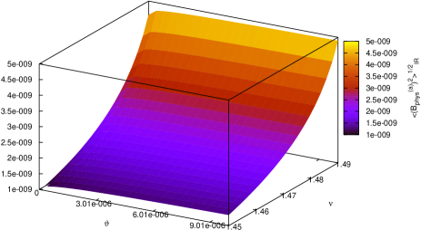
Figure 1: $\left.\left<\left(B^{(a)}_{phys}\right)^{2}\right>^{1/2}\right|_{IR}$ (in Gauss), with respect to $\nu$ and $\vartheta$. Notice that $\nu$ is related to the spectral index $n_{s}$ by the expression: $n_{s}=4-2\nu$, so that values used in the graphic for $\nu=(1.45,1.49)$ correspond respectively to $n_{s}=(1.1,1.02)$. Values considered for $\vartheta$ correspond to actual scales from $3\times 10^{3}$ to $3\times 10^{6}$ Mpc.

References

- (1) Y. Sofue, M. Fujimoto and R. Wielebinski, Ann. Rev. Astron. Astrophys. 24, 459 (1986).
- (2) E. Asseo and H. Sol, Phys. Rep. 148, 307 (1987).
- (3) P. P. Kronberg, Rep. Prog. Phys. 57, 325 (1994).
- (4) R. Beck, A. Brandenburg, D. Moss, A. A. Surkhurov and D. Sokloff, Annu. Rev. Astron. Astrophys. 34, 155 (1996).
- (5) D. Grasso and H. R. Bubinstein, Phys. Rep. 348, 163 (2001).
- (6) J. Bagchi, et al, New Astron. 7, 249 (2002).
- (7) P. P. Kronberg, J. J. Perri and A. L. Zukowski, Ap. J. 33, 528 (1992).
- (8) A. M. Wolfe, K. Lanzetta and A. L. Oren, Ap. J. 388, 17 (1992).
- (9) K.-T. Kim, P. C. Tribble and P. P. Kronberg, Astrophys. J. 379, 80 (1991).
- (10) M. Giovannini, Int. J. Mod. Phys. D13, 391 (2004).
- (11) C. Carilli and G. Taylor, Ann. Rev. Astron. Astrophys. 40, 319 (2002).
- (12) J. P. Vallée, Astron. J. 99, 459 (1990).
- (13) K. Subramanian and D. Barrow, Phys. Rev. D57, 3264 (1998).
- (14) C. G. Tsagas and J. D. Barrow, Class. Quantum Grav. 15, 3523 (1998); J. P. Ostriker, C. Thompson and E. Witten, Phys. Lett. B180, 231 (1986).
- (15) J. Vallée, Astron. J. 124, 1322 (2001).
- (16) A. Kosowsky, T. Kahniashvili, G. Lavrelashvili and B. Ratra, Phys. Rev. D71, 043006 (2005).
- (17) M. S. Turner and L. M. Widrow, Phys. Rev. D37, 2743 (1988).
- (18) A. D. Dolgov, Phys. Rev. D48, 2499 (1993); A. Ashoorioon, R. Mann, Phys. Rev. D71, 103509 (2005).
- (19) B. Ratra, Ap. J. 391, L1 (1992).
- (20) A. A. Starobinsky, JETP Lett. 30, 682 (1979); Phys. Lett. B91, 99 (1980).
- (21) A. Guth, Phys. Rev. D23, 347 (1981).
- (22) A. Linde, Phys. Lett. B129, 177 (1983).
- (23) D. S. Ledesma and M. Bellini, Phys. Lett. B581, 1 (2004).
- (24) J.E. Madriz Aguilar and M. Bellini, Phys. Lett. B619, 208 (2005).
- (25) J. E. Madriz Aguilar and M. Bellini, Eur. Phys. J. C38, 367 (2004).
- (26) 20 J.D. Jackson, Classical Electrodynamics, (John Wiley & Sons, Inc., 1975).
- (27) J. M. Overduin, P. S. Wesson, Phys. Rept. 283, 303 (1997).
- (28) C. A. Clarkson, A. A. Coley, R. Maartens and C. G. Tsagas, Class. Quant. Grav. 20, 1519 (2003).