Shear dynamics in Bianchi I cosmologies with $R^{n}$-gravity

Abstract

We give the equations governing the shear evolution in Bianchi spacetimes for general $f(R)$-theories of gravity. We consider the case of $R^{n}$-gravity and perform a detailed analysis of the dynamics in Bianchi I cosmologies which exhibit local rotational symmetry. We find exact solutions and study their behaviour and stability in terms of the values of the parameter $n$. In particular, we found a set of cosmic histories in which the universe is initially isotropic, then develops shear anisotropies which approaches a constant value.

leachj@maths.uct.ac.za, scarloni@maths.uct.ac.za and pksd@maths.uct.ac.za

1 Introduction

In the last few years there has been renewed interest in theories of gravity where the gravitational Lagrangian is a non-linear function of the scalar curvature. These $f(R)$-theories of gravity can take on a number of forms, the majority of the functions considered being of the type $R+\epsilon R^{m}$. Theories with $m=-1$ have been proposed as possible alternatives to sources of dark energy to explain the observed cosmic acceleration [1, 2]. Solar system experiments do however constrain these type of theories for any corrections higher than $R^{2}$ (quadratic gravity) [3]. In these theories corrections to the characteristic length scale of General Relativity (GR) are introduced through the addition of a new length scale which is determined by the constant $\epsilon$.

There are however forms of $f(R)$ which do not alter the characteristic length scale, for example $R^{n}$, in which GR is recovered when $n=1$. These $R^{n}$-gravity theories have many attractive features, such as simple exact solutions which allows for comparison with observations [4, 5]. There are however some caveats, in particular the stability and global behaviour of the underlying cosmological model is not well understood. The dynamical systems approach [6] can address some of these problems, since it provides one with exact solutions through the determination of fixed points and a (qualitative) description of the global dynamics of the system. Carloni et al [7] have recently used this method to study the dynamics of $R^{n}$-theories in Friedmann-Lemaître-Robertson-Walker (FLRW) universes. Clifton and Barrow [8] used the dynamical systems approach to determine the extent to which exact solutions can be considered as attractors of spatially flat universes at late times. They compared the predictions of these results with a range of observations and were able to show that the parameter $n$ in FLRW may only deviate from GR by a very small amount ($n-1\sim 10^{-19}$).

The dynamics of anisotropic models with $f(R)$-gravity have not been studied as intensively as their FLRW counterparts and it is therefore not known how the behaviour of the shear is modified in these theories of gravity. Bianchi spacetimes with isotropic 3-surfaces have been investigated for the quadratic theory [9] and it was found that in Bianchi I cosmologies the universe isotropises slower than in the Einstein case. The equations governing the evolution of shear in Bianchi spacetimes for general $f(R)$-theories can be found from the trace-free Gauss-Codazzi equations (see for example [10, 11]). However, it is not easy to solve these equations since the shear depends non-linearly on the Ricci scalar. Consequently the dynamical systems approach provides us with the best means of understanding the dynamics of these models.

In GR the vacuum Kasner solutions [12] and their fluid filled counterparts, the Type I Bianchi models, proved useful as a starting point for the investigation of the structure of anisotropic models. Barrow and Clifton [13, 14] have recently shown that it is also possible to find solutions of the Kasner type for $R^{n}$-gravity models. In [13] they showed that exact Kasner-like solutions do exist in the range of parameter $n$ for $1/2<n<5/4$ but with different Kasner-index relations to the ones in GR. In this paper we extend the dynamical systems analysis of $R^{n}$–gravity [7] to Bianchi I cosmological models that exhibit local rotational symmetry (LRS) [15, 16, 17]. LRS spacetimes geometries are subgroups within anisotropic spacetimes in which isotropies can occur around a point within the spacetime in 1- or 3–dimensions. Thus there exists a unique preferred spatial direction at each point which constitutes a local axis of symmetry. All observations are identical under rotation about the axis and are the same in all spatial directions perpendicular to that direction [15, 16].

Our analysis of the vacuum case revealed some interesting features regarding the evolution of Bianchi I cosmologies in HOTG. The phase space contains one isotropic fixed point and a line of fixed points with shear. The isotropic fixed point is an attractor (stable node) for values of the parameter $n$ in the ranges $n<1/2$, $1/2<n<1$ and $n>5/4$. In the range $1<n<5/4$ this point is a repeller (unstable node) and therefore may be seen as a past attractor. The existence of an isotropic past attractor implies, as in the case of braneworld models [18, 19, 20, 21], that we do not require special initial conditions for inflation to start since the cosmological singularity is FLRW. Another feature of these models is that the shear evolution is independent of the value of $n$ and is the same for all fixed points on the line.

The outline of this paper is as follows: In section 2 we give the basic equations for the kinematical and dynamical variables and we also state the field equations for general $f(R)$-theories of gravity. In section 3 we convert these equations into an autonomous set of equations for the case of $R^{n}$. We then proceed in section 4 and 5 to analyse this system for models with vacuum and matter respectively.

The following conventions will be used in this paper: the metric signature is $(-+++)$; Latin indices run from 0 to 3; $\nabla$ represents the usual covariant derivatives which may be split ($1+3$–covariantly) with the spatial covariant derivative being denoted by $D$ and the time derivative by a dot; units are used in which $c=8\pi G=1$.

2 Kinematics and dynamics of $f(R)$-gravity

2.1 Kinematical and dynamical quantities

We first state the relevant equations governing relativistic fluid dynamics (see for e.g. [10, 11]). For any given fluid 4-velocity vector field $u^{a}$, the projection tensor $h_{ab}=g_{ab}+u_{a}u_{b}$ projects into the instantaneous rest-space of a comoving observer. The first covariant derivative can be decomposed as

$$\nabla_{a}u_{b}=-\,u_{a}\,\dot{u}_{b}+D_{a}u_{b}=-\,u_{a}\,\dot{u}_{b}+{{\textstyle{1\over 3}}}\,\Theta\,h_{ab}+\sigma_{ab}+\omega_{ab}\ ,$$ (1)

where $\sigma_{ab}$ is the symmetric shear tensor ($\sigma_{ab}=\sigma_{(ab)}$, $\sigma_{ab}\,u^{b}=0$, $\sigma^{a}{}_{a}=0$), $\omega_{ab}$ is the vorticity tensor ($\omega_{ab}=\omega_{[ab]}$, $\omega_{ab}\,u^{b}=0$) and $\dot{u}_{a}$ is the acceleration vector ($\dot{u}_{a}=u^{b}\nabla_{b}u_{a}$). $\Theta$ is the volume expansion ($\Theta=\nabla_{a}u^{a}$) which defines a length scale $a$ along the flow lines via the standard relation $\Theta={\textstyle{3\dot{a}\over a}}$.

The matter energy-momentum tensor $T^{M}_{ab}$ can be decomposed relative to $u^{a}$ in the form

$$T^{M}_{ab}=\mu\,u_{a}\,u_{b}+q_{a}\,u_{b}+u_{a}\,q_{b}+p\,h_{ab}+\pi_{ab}\ ,$$

where $\mu$ is the relativistic energy density, $p$ the isotropic pressure, $q^{a}$ the energy flux ($q_{a}\,u^{a}=0$) and $\pi_{ab}$ the trace-free anisotropic pressure ($\pi^{a}{}_{a}=0$, $\pi_{ab}=\pi_{(ab)}$, $\pi_{ab}\,u^{b}=0$), all relative to $u^{a}$.

The conservation equations $\nabla^{b}T^{M}_{ab}=0$, can be split with respect to $u^{a}$ and $h_{ab}$:

$$\dot{\mu}+D_{a}q^{a}+\Theta(\mu+p)+2(\dot{u}_{a}q^{a})+(\sigma^{a}\!_{b}\pi^{b}\!_{a})=0,$$ (2)

$$\dot{q}^{\langle a\rangle}+D^{a}p+D_{b}\pi^{ab}+{\textstyle{4\over 3}}\Theta\,q^{a}+\sigma^{a}\!_{b}\,q^{b}+(\mu+p)\,\dot{u}^{a}-\dot{u}_{b}\,\pi^{ab}+\omega^{ab}q_{b}=0.$$ (3)

2.2 $f(R)$-gravity Field Equations

In the case where the gravitational Lagrangian is a non-linear function of the scalar curvature $f(R)$, the action reads

$${\cal A}=\int dx^{4}\sqrt{-g}f(R)+\int{\cal L}_{M}dx^{4},$$ (4)

where ${\cal L}_{M}$ is the Lagrangian of the matter fields. The fourth order field equations can be obtained by varying (4):

$$T^{M}_{ab}=f^{\prime}R_{ab}-{\textstyle{1\over 2}}fg_{ab}+S_{cd}\left(g^{cd}g_{ab}-g^{c}_{\;a}g^{d}_{\;b}\right),$$ (5)

where primes denote derivatives with respect to $R$ and $S_{ab}=\nabla_{a}\nabla_{b}f^{\prime}(R)$. $S_{ab}$ can be decomposed as

$$S_{ab}=f^{\prime\prime}D_{a}D_{b}R+f^{\prime\prime\prime}D_{a}R\;D_{b}R-f^{\prime\prime\prime}\dot{R}\left(D_{b}R\;u_{a}+D_{a}R\;u_{b}\right)+f^{\prime\prime\prime}\dot{R}^{2}\;u_{a}u_{b}$$

$$-f^{\prime\prime}\left[D_{a}\dot{R}\;u_{b}+u^{c}\nabla_{c}(D_{b}R)\;u_{a}\right]+f^{\prime\prime}\left[\ddot{R}\;u_{a}u_{b}-\dot{R}(D_{a}u_{b}-u_{a}\dot{u}_{b})\right],$$ (6)

and so the D’Lambertian can be given by

$$S=\square f^{\prime}(R)=g^{ab}\nabla_{a}\nabla_{b}f^{\prime}(R)$$

$$=f^{\prime\prime}D^{c}D_{c}R+f^{\prime\prime\prime}D^{c}R\;D_{c}R+f^{\prime\prime}\dot{u}^{c}D_{c}R-f^{\prime\prime}(\ddot{R}+\dot{R}\Theta)-f^{\prime\prime\prime}\dot{R}^{2}.$$ (7)

The field equation (5) can be rewritten in the standard form

$$R_{ab}-{\textstyle{1\over 2}}g_{ab}R=T^{TOT}_{ab},$$ (8)

(when $f^{\prime}(R)\neq 0$) where the effective stress energy momentum tensor $T^{TOT}_{ab}$ is given by

$$T^{TOT}_{ab}=f^{\prime-1}\left[T^{M}_{ab}+{\textstyle{1\over 2}}g_{ab}\left(f-f^{\prime}R\right)+S_{cd}\left(g^{c}_{\;a}g^{d}_{\;b}-g^{cd}g_{ab}\right)\right].$$ (9)

As pointed out in [7], no matter how complicated the effective stress energy momentum tensor for the HOTG system is, it is always divergence free if $\nabla^{b}T^{M}_{ab}=0$. The total conservation equations therefore have the same form as those for standard matter and can thus be represented by (2) and (3).

The higher order field equations may then be split (see [10, 9, 22]) to give the following contributions:

$$\hskip 28.45274ptR = f^{\prime\;-1}\left[3p-\mu+2f-3\,S\right],$$ (10)

$$R_{ab}u^{a}u^{b} = f^{\prime\;-1}\left[\mu-{\textstyle{1\over 2}}f+h^{ab}S_{ab}\right],$$ (11)

$$R_{ab}u^{a}h^{b}_{c} = f^{\prime\;-1}\left[-q_{c}+S_{ab}u^{a}h^{b}_{c}\right],$$ (12)

$$R_{ab}h^{a}_{c}h^{b}_{d} = f^{\prime\;-1}\left[\pi_{cd}-\left(p+{\textstyle{1\over 2}}f+S\right)h_{cd}+S_{ab}h^{a}_{c}h^{b}_{d}\right].$$ (13)

The propagation and constraint equations for $f(R)$-theories are given by Ripple et al. [22]. In what follows we will use the Raychaudhuri equation

$$\dot{\Theta}-D_{a}\dot{u}^{a}+{\textstyle{1\over 3}}\,\Theta^{2}-(\dot{u}_{a}\dot{u}^{a})+2\,\sigma^{2}-2\,\omega^{2}+f^{\prime\;-1}\left[\mu-{\textstyle{1\over 2}}f+h^{ab}S_{ab}\right]=0,$$ (14)

and the trace free Gauss-Codazzi equation, which holds for an irrotational matter fluid flow ($\omega_{ab}=0$):

$${}^{3}R_{ab}-{\textstyle{1\over 3}}({}^{3}R)h_{ab} = -\dot{\sigma}_{\langle ab\rangle}-\Theta\,\sigma_{ab}+D_{\langle a}\dot{u}_{b\rangle}+\dot{u}_{\langle a}\,\dot{u}_{b\rangle}+f^{\prime\;-1}\pi_{ab}$$ (15)

$$+f^{\prime\;-1}\left[h^{c}_{a}h^{d}_{b}-{\textstyle{1\over 3}}h_{ab}h^{cd}\right]S_{cd},$$

where the 3-Ricci scalar is given by

$$^{3}R=2\sigma^{2}-{\textstyle{2\over 3}}\Theta^{2}+f^{\prime\;-1}\left[\mu+3p+f-S+2h^{cd}S_{cd}\right].$$ (16)

3 Shear dynamics in Bianchi I cosmologies

3.1 $f(R)$-gravity

We consider a Bianchi spacetimes whose homogeneous hypersurfaces have isotropic 3-curvature ${}^{3}R_{ab}={\textstyle{1\over 3}}({}^{3}R)h_{ab}$. These spacetimes include the Bianchi models which, via the dissipation of the shear anisotropy $\sigma_{ab}$, can reach a FLRW limit. Spatial homogeneity implies that the spatial gradients will vanish and that $\dot{u}_{a}=0=\omega$. Thus the trace free Gauss-Codazzi equation (15) becomes

$$\dot{\sigma}_{\langle ab\rangle}+\Theta\,\sigma_{ab}=f^{\prime-1}\left[\pi_{ab}+\left(h^{c}_{a}h^{d}_{b}-{\textstyle{1\over 3}}h_{ab}h^{cd}\right)S_{cd}\right],$$ (17)

and $S_{ab}$ can be split as follows

$$S_{ab} = f^{\prime\prime}\left(\ddot{R}u_{a}u_{b}-\dot{R}\nabla_{b}u_{a}\right)+f^{\prime\prime\prime}\dot{R}^{2}u_{a}u_{b},$$ (18)

$$S_{ab}u^{a}u^{b} = f^{\prime\prime}\ddot{R}+f^{\prime\prime\prime}\dot{R}^{2},$$ (19)

$$S_{ab}h^{ab} = -f^{\prime\prime}\dot{R}\Theta,$$ (20)

$$S = -f^{\prime\prime}(\ddot{R}+\dot{R}\Theta)-f^{\prime\prime\prime}\dot{R}^{2}.$$ (21)

Substituting these components into the Gauss-Codazzi equation (17) gives

$$\dot{\sigma}_{\langle ab\rangle}+\Theta\,\sigma_{ab}=f^{\prime\;-1}\left[\pi_{ab}-f^{\prime\prime}\dot{R}\sigma_{\langle ab\rangle}\right].$$ (22)

In the case of a perfect matter fluid, $\pi_{ab}=0$, so that the equation above becomes

$$\dot{\sigma}_{\langle ab\rangle}+\Theta\,\sigma_{ab}=a^{-3}\frac{d}{d\tau}\left(a^{3}\,\sigma_{ab}\right)=-\frac{f^{\prime\prime}\dot{R}}{f^{\prime}}\sigma_{ab}.$$ (23)

On integration this yields

$$\sigma_{ab}=f^{\prime\;-1}\Psi_{ab}a^{-3},\ \ \ \ \ \dot{\Psi}_{ab}=0,$$ (24)

which in turn implies

$$\sigma^{2}=f^{\prime\;-2}\Psi^{2}a^{-6},\ \ \ \ \ \dot{\Psi}^{2}=0.$$ (25)

In the case of $f(R)=R$, equation (25) gives the standard GR solution (see [11] and references there in) whose behaviour can be summarised as follows:

$$\sigma^{2}\rightarrow\infty\ \ {\rm as}\ \ a\rightarrow 0,\ \ \ \ \sigma^{2}\rightarrow 0\ \ {\rm as}\ \ a\rightarrow\infty.$$

This behaviour is modified in $f(R)$-theories of gravity (see [23, 9]), because $R$ (and therefore $f^{\prime}$) is a function of $\sigma^{2}$ (see (29) below) and therefore (25) is implicit. In particular, the dissipation of the shear in Bianchi I spacetimes is slower in quadratic gravity than in GR [9]. However, this result was obtained by solving the evolution equations under the assumption that the scale factor also has a power-law evolution. Although this is desirable it may not necessarily be true since no analytical cosmological solution could be obtained in [9]. A more general approach to this problem is to make use of the theory of dynamical systems (see [6] and references therein). In the following we will apply this technique to $R^{n}$ gravity in order to investigate further the behaviour of the shear in this framework.

3.2 $R^{n}$– gravity

We begin by specialising all the evolution equations above to the case of $f(R)=R^{n}$. The Raychaudhuri equation (14) is now

$$\dot{\Theta}+{\textstyle{1\over 3}}\,\Theta^{2}+2\sigma^{2}-\frac{1}{2n}R-(n-1)\frac{\dot{R}}{R}\Theta+\frac{\mu}{nR^{n-1}}=0,$$ (26)

and the trace free Gauss-Codazzi equation (22) for LRS spacetimes is given by

$$\dot{\sigma}=-\left(\Theta+(n-1)\frac{\dot{R}}{R}\right)\sigma.$$ (27)

The Friedmann equation can be found from (16)

$${\textstyle{1\over 3}}\,\Theta^{2}-\sigma^{2}+(n-1)\frac{\dot{R}}{R}\Theta-\frac{(n-1)}{2n}R-\frac{\mu}{nR^{n-1}}=0.$$ (28)

In general, the substitution of the Friedmann equation (28) into the Raychaudhuri equation (26) yields

$$R=2\dot{\Theta}+{\textstyle{4\over 3}}\Theta^{2}+2\sigma^{2}.$$ (29)

Note that, in this relation the energy density does not appear explicitly, but is however still contained implicitly in the variables on the right hand side.

In this paper we will assume standard matter behaves like a perfect fluid with barotropic pressure $p=w\mu$. The conservation equation (2) in this case is

$$\dot{\mu}=-(1+w)\mu\Theta.$$ (30)

In order to convert the equations above into a system of autonomous first order differential equations, we define the following set of expansion normalised variables ;

$$\Sigma=\frac{3\sigma^{2}}{\Theta^{2}}\;,\ \ \ \ \ \ x=\frac{3\dot{R}}{R\Theta}(n-1)\;,$$ (31)

$$y=\frac{3R}{2n\Theta^{2}}(n-1)\;,\ \ \ \ \ \ z=\frac{3\mu}{nR^{n-1}\Theta^{2}}\;,$$

whose equations are

$$\Sigma^{\prime}=2\left(-2+2\Sigma-\frac{y}{n-1}-2x+z\right)\Sigma,$$

$$x^{\prime}=y(2+x)-\frac{y}{n-1}(2+nx)-2x-2x^{2}+xz+(1-3w)z+2x\Sigma,$$ (32)

$$y^{\prime}=\frac{y}{n-1}\left[(3-2n)x-2y+2(n-1)z+4(n-1)\Sigma+2(n-1)\right],$$

$$z^{\prime}=z\left[2z-(1+3w)-3x-\frac{2y}{n-1}+4\Sigma\right],$$

where primes denote derivatives with respect to a new time variable $\tau=\ln a$ and the dynamical variables are constrained by

$$1-\Sigma+x-y-z=0.$$ (33)

4 Dynamics of the vacuum case

We first consider the vacuum case ($\mu=0$). In this case the set of dynamical equations (3.2) are given by

$$\Sigma^{\prime} = 2\left(-2+2\Sigma-\frac{y}{n-1}-2x\right)\Sigma,$$

$$x^{\prime} = y(2+x)-\frac{y}{n-1}(2+nx)-2x-2x^{2}+2x\Sigma,$$ (34)

$$y^{\prime} = \frac{y}{n-1}\left[(3-2n)x-2y+4(n-1)\Sigma+2(n-1)\right],$$

together with the constraint equation

$$1-\Sigma+x-y=0.$$ (35)

4.1 Fixed points and solutions

The two most useful variables are $\Sigma$ and $y$ since they respectively represent a measure of the expansion normalised shear and the expansion normalised Ricci curvature and hence allow us to investigate how the shear is modified by the curvature. We can therefore simplify the system (4), by making use of the constraint (35), which allow us to write the equation for $x$ as a combination of the two variables $\Sigma$ and $y$:

$$\Sigma^{\prime} = -2\left(\frac{2n-1}{n-1}\right)\;y\;\Sigma,$$

$$y^{\prime} = \frac{y}{n-1}\left[(2n-1)\Sigma-(2n-1)y+(4n-5)\right],$$ (36)

which together with the constraint (35) represents our new system. Setting $\Sigma^{\prime}=0$ and $y^{\prime}=0$ we obtain one isotropic fixed point $\mathcal{A}:\ \left(0,{\textstyle{4n-5\over 2n-1}}\right)$ and a line of fixed points $\mathcal{L}_{1}:\ \left(\Sigma_{*},0\right)$ where $\Sigma_{*}\geq 0$ ($\Sigma_{*}<0$ would imply imaginary shear) . The point $\Sigma_{*}=0$ on $\mathcal{L}_{1}$ represents another isotropic fixed point that merges with $\mathcal{A}$ when $n=5/4$.

The fixed points may be used to find exact solutions for the Bianchi I models. We substitute the definitions (31) into (29) to obtain

$$\dot{\Theta}=\left(\frac{n}{n-1}y_{i}-\Sigma_{i}-2\right)\frac{\Theta^{2}}{3},$$ (37)

where $(\Sigma_{i},y_{i})$ represents the coordinates of the fixed points. Given that $n\neq 1$ and $ny_{i}-(n-1)\left(\Sigma_{i}+2\right)\neq 0$, this equation can be integrated to give

$$a=a_{0}\left(t-t_{0}\right)^{\alpha},\ \ \ {\rm where}\ \ \ \alpha=\left(2+\Sigma_{i}-{\textstyle{n\over n-1}}y_{i}\right)^{-1}.$$ (38)

In the case of the fixed point $\mathcal{A}$ we have

$$a=a_{0}\left(t-t_{0}\right)^{{\textstyle{(1-n)(2n-1)\over(n-2)}}},$$ (39)

which is the same as the solution found in [7].

For the fixed line $\mathcal{L}_{1}$ we have

$$a=a_{0}\left(t-t_{0}\right)^{{\textstyle{1\over 2+\Sigma_{*}}}},$$ (40)

but direct substitution into the cosmological equations reveals that this solution is only valid for $n>1$. For $n<1$ the fixed points on $\mathcal{L}_{1}$ are non physical because the field equations do not hold there. We have summarised these solution in Table 2.

Table 1: The fixed points and eigenvalues for $R^{n}$-gravity in a LRS Bianchi I vacuum model.

	Fixed points $(\Sigma,y)$	Eigenvalues
Point $\mathcal{A}$	$\left(0,{\textstyle{4n-5\over 2n-1}}\right)$	$\left[{\textstyle{2(5-4n)\over n-1}},{\textstyle{(5-4n)\over n-1}}\right]$
Line $\mathcal{L}_{1}$	$\left(\Sigma_{*},0\right)$	$\left[0,{\textstyle{(4n-5)\over n-1}}+{\textstyle{(2n-1)\over n-1}}\Sigma_{*}\right]$

Table 2: The solutions of the scale factor and shear evolution for $R^{n}$-gravity in a LRS Bianchi I vacuum model.

	Scale factor	Shear
Point $\mathcal{A}$	$a=a_{0}\left(t-t_{0}\right)^{{\textstyle{(1-n)(2n-1)\over(n-2)}}}$	$\sigma=0$
Line $\mathcal{L}_{1}$	$a=a_{0}\left(t-t_{0}\right)^{{\textstyle{1\over 2+\Sigma_{*}}}}$,   (only valid for $n>1$)	$\sigma=\sigma_{0}a^{-(2+\Sigma_{*})}$

The analysis above would be incomplete without determining the fixed points at infinity. In order for us to compactify the phase space, we transform our coordinates $(\Sigma,y)$ to polar coordinates

$$\Sigma=\bar{r}\cos\phi,\ \ \ \ \ y=\bar{r}\sin\phi$$ (41)

and set $\bar{r}=\frac{r}{1-r}$. Now since $\Sigma\geq 0$, we will only consider half of the phase space, i.e. $-\pi/2\leq\phi\leq\pi/2$. In the limit $r\rightarrow 1$ ($\bar{r}\rightarrow\infty$), equations (4.1) take on the form

$$r^{\prime} =\frac{(2n-1)}{4(n-1)}\left[\;\cos\phi-\cos 3\phi-5\sin\phi-\sin 3\phi\;\right],$$ (42)

$$\phi^{\prime} =\frac{(2n-1)\left[\cos\phi-\cos 3\phi+\sin\phi+\sin 3\phi\;\right]}{(n-1)(1-r)}.$$ (43)

Since (42) does not depend on $r$ we can find the fixed points by making use of (43) only. Setting $\phi^{\prime}=0$ we obtain four fixed points which are listed in Table 3 with their corresponding solutions.

Table 3: Asymptotic fixed points, $\phi$-coordinates and solutions for $R^{n}$-gravity in a LRS Bianchi I vacuum model.

Point	$\phi$	Scale factor	Shear
$\mathcal{A}_{\infty}$	$0$	$\tau-\tau_{\infty}=\frac{1}{\Sigma_{c}}\ln\left|t-t_{0}\right|+C$	$\sigma=\sigma_{0}a^{-(2+\Sigma_{c})}$
$\mathcal{B}_{\infty}$	${\textstyle{\pi\over 2}}$	$|\tau-\tau_{\infty}|=\left[C_{1}\pm C_{0}\left|{\textstyle{n-1\over 2n-1}}\right|(t-t_{0})\right]^{\frac{2n-1}{n-1}}$	$\sigma=0$
$\mathcal{C}_{\infty}$	${\textstyle{3\pi\over 2}}$	$|\tau-\tau_{\infty}|=\left[C_{1}\pm C_{0}\left|{\textstyle{n-1\over 2n-1}}\right|(t-t_{0})\right]^{\frac{2n-1}{n-1}}$	$\sigma=0$
$\mathcal{D}_{\infty}$	${\textstyle{7\pi\over 4}}$	$|\tau-\tau_{\infty}|=\left[C_{1}\pm C_{2}(t-t_{0})\right]^{2}$	$\sigma=\sigma_{0}$

The form of the scale factor can be determined from the fixed points by integrating (42) to find [8, 24]

$$r-1=g(\phi_{i})(\tau-\tau_{\infty}),$$ (44)

where $g(\phi_{i})$ represents the right hand side of (42) and $\tau\to\tau_{\infty}$ as $r\to 1$. The evolution equation (37) is then transformed into polar coordinates

$$\frac{\Theta^{\prime}}{\Theta}=\frac{r}{1-r}\left(\frac{n}{n-1}\sin\phi_{i}-\cos\phi_{i}-\frac{2(1-r)}{r}\right),$$ (45)

which in the limit $r\to 1$ take on the form

$$\frac{\Theta^{\prime}}{\Theta}=\frac{-1}{g(\phi_{i})(\tau-\tau_{\infty})}\left(\frac{n}{n-1}\sin\phi_{i}-\cos\phi_{i}\right).$$ (46)

The equations above were all given in terms of the new time variable $\tau$ by using the relation $\Theta^{\prime}=3\dot{\Theta}/\Theta$. Integrating (46) yields the solution

$$|\tau-\tau_{\infty}|=\left[C_{1}\pm C_{0}\left|h(\phi_{i})\right|(t-t_{0})\right]^{\textstyle{1\over h(\phi_{i})}},$$ (47)

where

$$h(\phi_{i})=\frac{1}{g(\phi_{i})}\left(\frac{n}{n-1}\sin\phi_{i}-\cos\phi_{i}\right)+1.$$ (48)

Solutions at infinity can now be obtained by directly substituting the fixed points into (47), so for points $\mathcal{B}_{\infty}$ and $\mathcal{C}_{\infty}$ we find

$$|\tau-\tau_{\infty}|=\left[C_{1}\pm C_{0}\left|\frac{n-1}{2n-1}\right|(t-t_{0})\right]^{\frac{2n-1}{n-1}},$$ (49)

and for point $\mathcal{D}_{\infty}$

$$|\tau-\tau_{\infty}|=\left[C_{1}\pm C_{2}(t-t_{0})\right]^{2}.$$ (50)

The solution at point $\mathcal{A}_{\infty}$ can not be determined with this method since the limit approaches our fixed line $\mathcal{L}_{1}$ so that (47) yields an indefinite solution. However, defining the two new variables: $S=\ln\Sigma$ and $Y=\ln y$, the system (4.1) can be written as

$$S^{\prime} = -2\left(\frac{2n-1}{n-1}\right)\;e^{Y},$$

$$Y^{\prime} = \left(\frac{2n-1}{n-1}\right)\left(e^{S}-e^{Y}\right)+\left(\frac{4n-5}{n-1}\right).$$ (51)

Point $\mathcal{A}_{\infty}$ corresponds to $y\to 0$ as $\Sigma\to\infty$, so in its neighborhood the system (4.1) reduces to

$$S^{\prime}=0\ \ \ \ {\rm and}\ \ \ \ Y^{\prime}=\left(\frac{2n-1}{n-1}\right)e^{S},$$ (52)

which has the solution

$$S=S_{c}=constant\ \ \ \ {\rm and}\ \ \ \ Y=\left(\frac{2n-1}{n-1}\right)e^{S_{c}}\left(\tau-\tau_{\infty}\right).$$ (53)

The form of the scale factor for $\mathcal{A}_{\infty}$ can then be found in the same way as the previous points. For $y\to 0$ as $\Sigma\to\infty$, (37) takes the form $\dot{\Theta}=-\Sigma_{c}\frac{\Theta^{2}}{3}$ where $\Sigma_{c}=e^{S_{c}}$. We find the solution as

$$\tau-\tau_{\infty}=\frac{1}{\Sigma_{c}}\ln\left|t-t_{0}\right|+C,$$ (54)

where $C$ is a constant of integration.

4.2 Stability of the fixed points

The stability of the fixed point may be determined by linearising the system of equation (4.1). This can be done by perturbing $\Sigma$ and $y$ around the fixed points $(\Sigma_{i},y_{i})$ via $\Sigma=\Sigma_{i}+\delta\Sigma$ and $y=y_{i}+\delta y$. The corresponding eigenvalues of the linearised system are given in Table 1. The fixed point $\mathcal{A}$ is an unstable node (repeller) for values of $n$ in the range $1<n<5/4$. For all other values of $n$ it is a stable node (attractor).

The fixed points on line $\mathcal{L}_{1}$ all contain at least one zero eigenvalue and therefore we will have to study the effect of small perturbations around the line. We find that they have the following solutions

$$\delta\Sigma=\frac{\kappa}{\eta}e^{\eta\tau},\hskip 28.45274pt\delta y=C\;e^{\eta\tau},$$ (55)

where $C$ is a constant of integration and

$$\eta=\frac{(2n-1)}{(n-1)}\Sigma_{*}+\frac{(4n-5)}{(n-1)},\ \ \ \ \ \ \kappa=-\frac{2(2n-1)}{(n-1)}.$$ (56)

In order for the fixed points on line $\mathcal{L}_{1}$ to be stable node, we must have $\eta<0$. The fixed point is an unstable node when $\eta>0$. Over the interval $0\leq\Sigma_{*}<\frac{5-4n}{2n-1}$, we will have stable nodes for $1<n<5/4$ and unstable nodes for $1/2<n<1$. The remainder of the points $\Sigma_{*}>\frac{5-4n}{2n-1}$, will be stable nodes for $1/2<n<1$ and unstable nodes for $1<n<5/4$. When $n<1/2$ and $n>5/4$, the fixed points are always unstable nodes. We also note that for $\Sigma_{*}=1$, $\eta=6$ and is therefore always an unstable node. The stability of all the fixed points is given in Table 4.

Table 4: Stability of the fixed points for $R^{n}$-gravity in a LRS Bianchi I vacuum model. We use the term ‘attractor’ to denote a stable node and ‘repeller’ refers to an unstable node.

	$n<1/2$	$1/2<n<1$	$1<n<5/4$	$n>5/4$
Point $\mathcal{A}$	attractor	attractor	repeller	attractor
Line $\mathcal{L}_{1}$
$\Sigma_{*}=1$	repeller	repeller	repeller	repeller
$0\leq\Sigma_{*}<\frac{5-4n}{2n-1}$	repeller	repeller	attractor	repeller
$\Sigma_{*}>\frac{5-4n}{2n-1}$	repeller	attractor	repeller	repeller

A similar analysis may be performed for the fixed points at infinity. We only need to perturb the angular variable $\phi$ around the fixed points $\phi_{i}$ via $\phi=\phi_{i}+\delta\phi$. The fixed points will be stable if $r^{\prime}>0$ and the eigenvalue $\lambda<0$ for the linearised equation $\delta\phi^{\prime}=\lambda\;\delta\phi$, in the limit of $\bar{r}\to\infty$. When both conditions are satisfied the point is an stable node, if only one is satisfied it is a saddle and when neither holds it is an unstable node. Substituting the expression above into (43) and linearising as before, yields

$$\delta\phi^{\prime}\approx\frac{(2n-1)}{4(n-1)(1-r)}\left[\;-\sin\phi_{i}+3\sin 3\phi_{i}+\cos\phi_{i}+3\cos 3\phi_{i}\;\right]\;\delta\phi.$$ (57)

The stability of the fixed points are summarised in Table 5. We see that only point $\mathcal{D}_{\infty}$ have stable nodes for $n<1/2$ and $n>1$. Points $\mathcal{B}_{\infty}$ and $\mathcal{C}_{\infty}$ are always saddle points and $\mathcal{A}_{\infty}$ is a saddle when $1/2<n<1$ but is otherwise an unstable node.

Table 5: Stability of the asymptotic fixed points for $R^{n}$-gravity in a LRS Bianchi I vacuum model. We use the term ‘saddle’ to denote a saddle node.

Point	$n<1/2$	$1/2<n<1$	$n>1$
$\mathcal{A}_{\infty}$	repeller	saddle	repeller
$\mathcal{B}_{\infty}$	saddle	saddle	saddle
$\mathcal{C}_{\infty}$	saddle	saddle	saddle
$\mathcal{D}_{\infty}$	attractor	repeller	attractor

4.3 Evolution of the shear

In the previous section we found two isotropic points; the fixed point $\mathcal{A}$ and one point on the fixed line at $\Sigma_{*}=0$. The remaining fixed points all have non-vanishing shear.

The trace free Gauss Codazzi equation (27) can in general (i.e. for all points in the phase space) be represented in terms of the dynamical variables (31) as

$$\frac{\dot{\sigma}}{\sigma}=-{\textstyle{1\over 3}}(2+\Sigma+y)\Theta.$$ (58)

From the equation above it is clear that the shear evolution for all points in the phase space that lie on the line $y=1-\Sigma$, is the same as in the case of GR. The shear will dissipate faster than in GR when $\dot{\sigma}/\sigma<-\Theta$, that is all points that lie in the region $y<1-\Sigma$. We will call this the fast shear dissipation (FSD) regime. When $\dot{\sigma}/\sigma>-\Theta$ and hence for all points in the region $y>1-\Sigma$, the shear will dissipate slower than in GR. This will be called the slow shear dissipation (SSD) regime.

The fixed points on $\mathcal{L}_{1}$ for which $\Sigma_{*}>0$ all have non-vanishing shear. For these points (58) has the form

$$\frac{\dot{\sigma}}{\sigma}=-{\textstyle{1\over 3}}(2+\Sigma_{*})\Theta=-(2+\Sigma_{*})\left(\frac{\dot{a}}{a}\right),$$ (59)

which may be integrated to give

$$\sigma=\sigma_{0}a^{-(2+\Sigma_{*})}=\sigma_{0}a_{0}^{-(2+\Sigma_{*})}(t-t_{0})^{-1},$$ (60)

where we made use of (40). We note that the final solution of the shear for these fixed points (60), does not depend on the parameter $n$. This is to be expected since both the coordinates of the points on $\mathcal{L}_{1}$ and equation (58) are independent of $n$.

The only other fixed point with non-vanishing shear is $\mathcal{D}_{\infty}$ which corresponds to $y\to-\infty$ as $\Sigma\to\infty$. In this limit (58) yields $\dot{\sigma}/\sigma=0$ which implies that $\sigma=\sigma_{0}$ (i.e. constant shear).

We first consider values of the parameter for which $n<1/2$ (see Figure 1). If the initial conditions of the universe lie in the region $y>0$ (negative Ricci scalar), the orbits will always approach the isotropic fixed point $\mathcal{A}$. The shear will dissipate slower than in GR for almost all the orbits in this region, apart from the ones below the dotted line $y=1-\Sigma$, which make the transition from the SSD region to the FSD region. When the initial conditions lie in the region $y<0$ (positive Ricci scalar), the orbits will approach the fixed point $\mathcal{D}_{\infty}$ which has constant shear.

The case $1/2<n<1$ is illustrated in Figures 2 and 3. If the initial conditions are such that they lie in the shaded area ($y<1-\Sigma$ and $y<0$), then the evolution will always be in the FSD regime and will approach the isotropic solution of the point $\mathcal{A}$. Instead, the unshaded area $y<0$ and $y>1-\Sigma$, is divided into two regions; the first one is located below the dash-dotted line and the second above the dash-dotted line. For initial conditions that lie in the first region, the orbits make a transition from the SSD region to the FSD region where they approach the point $\mathcal{A}$. When the initial conditions lie in the second region, the orbits will always lie in the SSD region and approach $\mathcal{L}_{1}$. When the initial conditions lie in $y<1-\Sigma$ and $y>0$, the universe will evolve from the FSD regime to the SSD regime, in which the evolution will approach the stable solutions on $\mathcal{L}_{1}$. In the remaining area where $y>1-\Sigma$ and $y>0$, the shear will always dissipate slower than in GR.

We next consider $1<n<5/4$ which is illustrated in Figure 4. If the initial conditions of the universe are such that they lie in the shaded area, then the shear will always dissipate faster than in the case of GR. When the initial conditions lie in the region $y>1-\Sigma$ and $y>0$, the universe will evolve from the SSD regime to the FSD regime and the evolution will approach the stable solutions on $\mathcal{L}_{1}$. If the initial conditions lie in the unshaded area of $y<0$, the orbits will approach the fixed point $\mathcal{D}_{\infty}$. For initial conditions that lie in the region $y<1-\Sigma$, there will be a transition from the FSD region to the SSD region. For all initial conditions that lie in the region $y<1-\Sigma$, the orbits always lie in the SSD region. We can see that for this range of $n$, the fixed point $\mathcal{A}$ acts as a past attractor. This is an interesting feature since an isotropic past attractor implies that unlike GR, where the generic cosmological singularity is anisotropic, we have initial conditions which corresponds to a FLRW spacetime. This feature was also found in the braneworld scenarios where it was shown that homogeneous and anisotropic braneworld models (and some simple inhomogeneous models) have FLRW past attractors (see e.g. [18, 19, 20, 21]). This means that although inflation is still required to produce the fluctuations observed in the cosmic microwave background (CMB), there is no need for special initial conditions for inflation to begin [25]. In the range $1<n<5/4$, we can obtain models whose evolution starts at the isotropic point $\mathcal{A}$ and then either evolves toward the fixed points ($\Sigma_{*},0$) on line $\mathcal{L}_{1}$ or towards the point $\mathcal{D}_{\infty}$. The orbits that approach $\mathcal{L}_{1}$ will always lie in the FSD region. The orbits which approach $\mathcal{D}_{\infty}$ will make a transition from the FSD region to the SSD region. An interesting set of orbits are the ones that approach the fixed points on $\mathcal{L}_{1}$ for which $(\sigma/H)_{*}<<1$. These cosmic histories represent an universe that is initially isotropic and then develops shear anisotropies which approach a constant value that can be chosen to be comparable with the expansion normalised shear observed today ($(\sigma/H)_{*}<10^{-9}$ [26, 27, 28]) . Inflation is therefore not required to explain the low degree of anisotropy observed in the CMB. Furthermore, we still require all other observational constraints to be satisfied.

Finally, we consider values in the range $n>5/4$ (see Figure 5). For all initial conditions that lie in the shaded region, the shear will always dissipate faster than in the case of GR; for $y>0$ the orbits will approach $\mathcal{A}$ and for $y<0$ approach the point $\mathcal{D}_{\infty}$. If initial conditions lie in the region $y>1-\Sigma$ and $y>0$, the orbits will initially be in the SSD region, and then approach the isotropic solution $\mathcal{A}$, which is in the FSD region. For all orbits in the region $y>1-\Sigma$ and $y<0$, the shear will always dissipate slower than in the case of GR.

Figure 1: Phase space of the vacuum LRS Bianchi model with $n<1/2$.

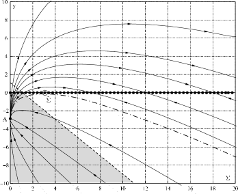
Figure 2: Phase space of the vacuum LRS Bianchi model with $1/2<n<1$ and where $\tilde{\Sigma}=\frac{5-4n}{2n-1}$. The shaded region represents the region of initial conditions for which the shear will always evolve faster than in GR.

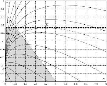
Figure 3: Close-up of the phase space of the vacuum LRS Bianchi model with $1/2<n<1$ around the line $y=1-\Sigma$.

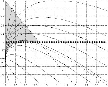
Figure 4: Phase space of the vacuum LRS Bianchi model with $1<n<5/4$.

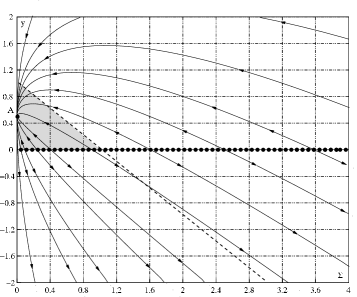
Figure 5: Phase space of the vacuum LRS Bianchi model with $n>5/4$.

5 Dynamics of the matter case

We will now consider the dynamics of LRS Bianchi I models in the presence of matter. As noted in [7], in HOTG there is a difference between vacuum and non-vacuum physics in the sense that not all higher order couplings are consistent in the presence of standard matter. This can be seen in the evolution equations (26) and (28) where the matter terms are coupled with a generic power of the curvature. Since the sign of the Ricci scalar is not fixed, these terms will not be defined for every real value of $n$. Thus, the inclusion of matter induces a natural constraint through the field equations on $R^{n}$- gravity and it is therefore necessary to express the results in terms of the allowed set of values of $n$. Following [7], we will work as if $n$ is unconstrained, supposing that the intervals we devise are meant to represent the subset of allowed values within these intervals.

Similar to the vacuum case, we can reduce the system (3.2) to the three variables $\Sigma$, $y$ and $z$ by making use of the constraint (33);

$$\Sigma^{\prime}=-2\left[\left(\frac{2n-1}{n-1}\right)\;y+z\right]\Sigma,$$

$$y^{\prime}=\frac{y}{n-1}\left[(2n-1)\Sigma-(2n-1)y+z+(4n-5)\right],$$ (61)

$$z^{\prime}=z\left[(2-3w)-z+\Sigma-\left(\frac{3n-1}{n-1}\right)\;y\right].$$

We note that when $y=0$ then $y^{\prime}=0$ and when $z=0$, $z^{\prime}=0$. The two planes $y=0$ and $z=0$ therefore corresponds to two invariant submanifolds. When $z=0$, the system (5) reduces to system (4.1) and one would be tempted to consider the plane $z=0$ as the vacuum invariant submanifold of the phase space, which would not be entirely correct. To illustrate this point, we write the energy density in terms of our expansion normalised variables (31)

$$\mu\propto zy^{n-1}\Theta^{2n}.$$ (62)

From this relation it can be seen that when $z=0$ and $y\neq 0$ the energy density is zero. However when $y=0$ and $z\neq 0$ the behaviour of $\mu$ does depend on the value of $n$. In this case the energy density is zero when $n>1$ but is divergent when $n<1$. When both $y$ and $z$ are equal to zero and $n<1$, one can only determine the behaviour of $\mu$ by direct substitution into the cosmological equations.

5.1 Fixed points and solutions

Setting $\Sigma^{\prime}=0$, $y^{\prime}=0$ and $z^{\prime}=0$ we obtain three isotropic fixed points $\mathcal{A}$, $\mathcal{B}$, $\mathcal{C}$ and a line of fixed points $\mathcal{L}_{1}:\ \left(\Sigma_{*},\ 0,\ 0\right)$, where $\Sigma_{*}\geq 0$ (see Table 6). When $\Sigma_{*}=0$ we have another isotropic fixed point which merges with $\mathcal{A}$ when $n=5/4$ and with $\mathcal{B}$ when $w=2/3$. This point will merge with $\mathcal{C}$ when $n=5/4$ and $w=2/3$.

We again substitute the definitions (31) into (29) to obtain

$$\dot{\Theta}=\left(\frac{n}{n-1}y_{i}-\Sigma_{i}-2\right)\frac{\Theta^{2}}{3}.$$ (63)

Under the condition that $n\neq 1$ and the terms inside the brackets are not equal to zero, this equation may be integrated to give the following solution

$$a=a_{0}\left(t-t_{0}\right)^{\alpha},\ \ \ {\rm where}\ \ \ \alpha=\left(2+\Sigma_{i}-{\textstyle{n\over n-1}}y_{i}\right)^{-1}.$$ (64)

The point $\mathcal{A}$ and line $\mathcal{L}_{1}$ will all have the same solutions as in the vacuum case, since either $y=0$ or $z=0$ for these points.

The behaviour of the scale factor for point $\mathcal{B}$ is

$$a=a_{0}\left(t-t_{0}\right)^{1/2},$$ (65)

and since $y_{2}=0$ and $z_{2}\neq 0$, the energy density is zero (only valid for $n>1$). When $n<1$, point $\mathcal{B}$ and the points on $\mathcal{L}_{1}$ are non physical since the energy density is divergent.

For point $\mathcal{C}$, the scale factor behaves as

$$a=a_{0}\left(t-t_{0}\right)^{{\textstyle{2n\over 3(1+w)}}},$$ (66)

while the energy density is

$$\mu=\mu_{0}t^{-2n},$$ (67)

where

$$\mu_{0} = (-1)^{n}3^{-n}2^{2n-1}n^{n}(1+w)^{-2n}(4n-3(1+w))^{n-1}$$

$$\times\left[2n^{2}(4+3w)-n(13+9w)+3(1+w)\right].$$

This point thus represents a power-law regime which in the case of $n>0$, yields an expanding solution with the energy density decreasing in time. In the case of $n<0$ we obtain a contracting solution with $\mu$ increasing in time. In order for $\mathcal{C}$ to be a physical point, we require $\mu>0$ and therefore $\mu_{0}>0$ (see [7] for detailed analysis). Note than when $n>{\textstyle{3\over 2}}(1+w)$, this solution corresponds to accelerated expansion.

Table 6: Fixed points and solutions of the scale factor and matter density for LRS Bianchi I with matter.

Point	Fixed points $(\Sigma,y,z)$	Scale factor	Matter density
$\mathcal{A}$	$\left(0,\;{\textstyle{4n-5\over 2n-1}},\;0\right)$	$a=a_{0}\left(t-t_{0}\right)^{{\textstyle{(1-n)(2n-1)\over(n-2)}}}$	$\mu=0$
$\mathcal{B}$	$\left(0,\;0,\;2-3w\right)$	$a=a_{0}\left(t-t_{0}\right)^{\frac{1}{2}}$	$\mu=0$   ($n>1$)
$\mathcal{C}$	$\left(0,\ \frac{(n-1)[4n-3(1+w)]}{2n^{2}},\right.$	$a=a_{0}\left(t-t_{0}\right)^{{\textstyle{2n\over 3(1+w)}}}$	$\mu=\mu_{0}t^{-2n}$
	$\left.\frac{n(13+9w)-2n^{2}(4+3w)-3(1+w)}{2n^{2}}\right)$
Line $\mathcal{L}_{1}$	$\left(\Sigma_{*},0,0\right)$	$a=a_{0}\left(t-t_{0}\right)^{{\textstyle{1\over 2+\Sigma_{*}}}}$	$\mu=0$  ($n>1$)

We next study the behaviour of the system (5) at infinity. The compactification of the phase space can be achieved by transforming to spherical coordinates

$$\Sigma=\bar{r}\sin\theta\cos\phi,\ \ \ \ y=\bar{r}\sin\theta\sin\phi,\ \ \ \ z=\bar{r}\cos\theta,$$ (68)

and setting $\bar{r}=\frac{r}{1-r}$, where $0\leq\bar{r}\leq\infty$, $0\leq\theta\leq\pi$ and since we are again only considering half of the phase space, $-\pi/2\leq\phi\leq\pi/2$ . In the limit $r\rightarrow 1$ ($\bar{r}\rightarrow\infty$), equations (5) take on the form

$$r^{\prime}=\frac{1}{4(n-1)}\left[\;2\cos\theta\{3-2n+(2n-1)\cos 2\phi\}+2\cos^{3}\theta\{(2n-1)\cos 2\phi-1\}\right.$$

$$\hskip 14.22636pt+2\sin\theta\;\cos^{2}\theta\{(2n-1)\cos 2\phi-1\}\{\cos\phi+\sin\phi\}$$

$$\hskip 14.22636pt+(2n-1)\sin\theta\left.\{\cos\phi-\cos 3\phi-5\sin\phi-\sin 3\phi\}\;\right],$$ (69)

$$\theta^{\prime}=\frac{\sin 2\theta\{1-(2n-1)\cos 2\phi\}\left[\cos\theta+\sin\theta\{\cos\phi+\sin\phi\}\;\right]}{4(n-1)(1-r)}$$ (70)

$$\phi^{\prime}=\frac{(2n-1)\sin 2\phi\left[\cos\theta+\sin\theta\{\cos\phi+\sin\phi\}\;\right]}{2(n-1)(1-r)}.$$ (71)

Table 7: Eigenvalues and shear solutions for LRS Bianchi I with matter.

Point	Eigenvalues	Shear
$\mathcal{A}$	$\left[{\textstyle{2(5-4n)\over n-1}},\;{\textstyle{5-4n\over n-1}},\;{\textstyle{n(13+9w)-2n^{2}(4+3w)-3(1+w)\over 1-3n+2n^{2}}}\right]$	$\sigma=0$
$\mathcal{B}$	$\left[-2+3w,\;-4+6w,\;{\textstyle{4n-3(1+w)\over n-1}}\right]$	$\sigma=0$
$\mathcal{C}$	$\left[{\textstyle{3((2n-1)w-1)\over n}},\;{\textstyle{P_{1}(n,w)-\sqrt{P_{2}(n,w)}\over 4n(n-1)}},\;{\textstyle{P_{1}(n,w)+\sqrt{P_{2}(n,w)}\over 4n(n-1)}}\right]$	$\sigma=0$
	$P_{1}(n,w)=3(1+w)+3n\left((2n-3)w-1\right)$
	$P_{2}(n,w)=(n-1)\left[4n^{3}(8+3w)^{2}-4n^{2}(152+3w(55+18w))\right.$
	$\left.+3n(1+w)(139+87w)-81(1+w)^{2}\right]$
Line $\mathcal{L}_{1}$	$\left[0,\;{\textstyle{(4n-5)\over n-1}}+{\textstyle{(2n-1)\over n-1}}\Sigma_{*},\;2-3w+\Sigma_{*}\right]$	$\sigma=\sigma_{0}a^{-(2+\Sigma_{*})}$

Now since (69) does not depend on $r$ we can find the fixed points by just making use of (70) and (71). Setting $\theta^{\prime}=0$ and $\phi^{\prime}=0$ we obtain the fixed points which are listed in Table 8 with their corresponding solutions.

Table 8: Coordinates and solutions of the asymptotic fixed points for LRS Bianchi with matter. For the fixed line $\tilde{\theta}=\arctan[-1/(\cos\phi_{i}+\sin\phi_{i})]$ and for the double point $\tilde{\phi}=(1/2)\arccos[1/(2n-1)]$.

Point	$(\theta,\phi)$	Scale factor	Shear
$\mathcal{A}_{\infty}$	$(0,0)$	$|\tau-\tau_{\infty}|=\left[C_{1}\pm C_{0}(t-t_{0})\right]$	$\sigma=0$
$\mathcal{B}_{\infty}$	$(\pi,0)$	$|\tau-\tau_{\infty}|=\left[C_{1}\pm C_{0}(t-t_{0})\right]$	$\sigma=0$
$\mathcal{C}_{\infty}$	$({\textstyle{\pi\over 2}},0)$	$\tau-\tau_{\infty}=\frac{1}{\Sigma_{c}}\ln\left|t-t_{0}\right|+C$	$\sigma=\sigma_{0}a^{-(2+\Sigma_{c})}$
$\mathcal{D}_{\infty}$	$({\textstyle{\pi\over 2}},{\textstyle{\pi\over 2}})$	$|\tau-\tau_{\infty}|=\left[C_{1}\pm C_{0}\left|{\textstyle{n-1\over 2n-1}}\right|(t-t_{0})\right]^{\frac{2n-1}{n-1}}$	$\sigma=0$
$\mathcal{E}_{\infty}$	$({\textstyle{\pi\over 2}},{\textstyle{3\pi\over 2}})$	$|\tau-\tau_{\infty}|=\left[C_{1}\pm C_{0}\left|{\textstyle{n-1\over 2n-1}}\right|(t-t_{0})\right]^{\frac{2n-1}{n-1}}$	$\sigma=0$
$\mathcal{F}_{\infty}$	$(\tilde{\theta},\tilde{\phi})$	$|\tau-\tau_{\infty}|=\left[C_{1}\pm C_{2}(t-t_{0})\right]^{2}$	$\sigma=\sigma_{0}$
Line
$\mathcal{L}_{\infty}$	$(\tilde{\theta},\phi)$	$|\tau-\tau_{\infty}|=\left[C_{1}\pm C_{2}(t-t_{0})\right]^{2}$	$\sigma=\sigma_{0}$

The form of the scale factor can be determined from the fixed points as in the vacuum case. We integrate (69) to find

$$r-1=G(\theta_{i},\phi_{i})(\tau-\tau_{\infty}),$$ (72)

where $G(\theta_{i},\phi_{i})$ represents the right hand side of (69) and $\tau\to\tau_{\infty}$ as $r\to 1$. We transform the evolution equation (63) to polar coordinates and write them in terms of the time parameter $\tau$:

$$\frac{\Theta^{\prime}}{\Theta}=\frac{r\;\sin\theta_{i}}{1-r}\left(\frac{n}{n-1}\sin\phi_{i}-\cos\phi_{i}-\frac{2(1-r)}{r\;\sin\theta_{i}}\right),$$ (73)

which in the limit $r\to 1$ takes the form

$$\frac{\Theta^{\prime}}{\Theta}=\frac{-\sin\theta_{i}}{G(\theta_{i},\phi_{i})(\tau-\tau_{\infty})}\left(\frac{n}{n-1}\sin\phi_{i}-\cos\phi_{i}\right).$$ (74)

Integrating the equation above then yields

$$|\tau-\tau_{\infty}|=\left[C_{1}\pm C_{0}\left|H(\theta_{i},\phi_{i})\right|(t-t_{0})\right]^{\textstyle{1\over H(\theta_{i},\phi_{i})}},$$ (75)

where

$$H(\theta_{i},\phi_{i})=\frac{\sin\theta_{i}}{G(\theta_{i},\phi_{i})}\left(\frac{n}{n-1}\sin\phi_{i}-\cos\phi_{i}\right)+1.$$ (76)

The solutions is then obtained by directly substituting the coordinates of the fixed points into (75). For points $\mathcal{A}_{\infty}$ and $\mathcal{B}_{\infty}$ we have the solutions

$$|\tau-\tau_{\infty}|=\left[C_{1}\pm C_{0}(t-t_{0})\right],$$ (77)

and for point $\mathcal{D}_{\infty}$ and $\mathcal{E}_{\infty}$ we have

$$|\tau-\tau_{\infty}|=\left[C_{1}\pm C_{0}\left|\frac{n-1}{2n-1}\right|(t-t_{0})\right]^{\frac{2n-1}{n-1}}.$$ (78)

In addition to the ordinary fixed points, we have a line of fixed points $\mathcal{L}_{\infty}$ for which $\tilde{\theta}=\arctan[-1/(\cos\phi_{i}+\sin\phi_{i})]$, and a double fixed point at $\tilde{\phi}=(1/2)\arccos[1/(2n-1)]$. Equation (75) gives the solutions for the fixed points on the line:

$$|\tau-\tau_{\infty}|=\left[C_{1}\pm C_{2}(t-t_{0})\right]^{2}.$$ (79)

As in the vacuum case, $\mathcal{C}_{\infty}$ can not be determined with this method since the limit approaches the fixed line $\mathcal{L}_{1}$. In order to analyse this point, we can define three new variables: $S=\ln\Sigma$, $Y=\ln y$ and $Z=\ln z$. The system (5) can then be written as

$$S^{\prime} = -2\left(\frac{2n-1}{n-1}\right)\;e^{Y}-2e^{Z},$$

$$Y^{\prime} = \left(\frac{2n-1}{n-1}\right)\left(e^{S}-e^{Y}\right)+\frac{1}{n-1}e^{Z}+\left(\frac{4n-5}{n-1}\right),$$ (80)

$$Z^{\prime} = (2-3w)-e^{Z}+e^{S}-\left(\frac{3n-1}{n-1}\right)e^{Y}.$$

The point $\mathcal{C}_{\infty}$ corresponds to $y\to 0$ and $z\to 0$ as $\Sigma\to\infty$ so that the system (5.1) reduce to

$$S^{\prime}=0,\ \ \ \ \ Y^{\prime}=\left(\frac{2n-1}{n-1}\right)e^{S},\ \ \ \ \ Z^{\prime}=e^{S},$$ (81)

which has the following solution

$$S=S_{c},\ \ \ Y=\left(\frac{2n-1}{n-1}\right)e^{S_{c}}\left(\tau-\tau_{\infty}\right),\ \ \ {\rm and}\ \ \ Z=e^{S_{c}}\left(\tau-\tau_{\infty}\right),$$ (82)

where $S_{c}$ is a constant. The form of the scale factor for $\mathcal{C}_{\infty}$ can then be found in the same way as the previous points. For $y\to 0$ and $z\to 0$ as $\Sigma\to\infty$, (63) takes the form $\dot{\Theta}=-\Sigma_{c}\frac{\Theta^{2}}{3}$ where $\Sigma_{c}=e^{S_{c}}$. We find the solution as

$$\tau-\tau_{\infty}=\frac{1}{\Sigma_{c}}\ln\left|t-t_{0}\right|+C,$$ (83)

where $C$ is a constant of integration.

5.2 Stability of the fixed points

We next check the stability of the fixed point by linearising the system of equation (5). The eigenvalues of the linearised system are given in Table 7.

For the stability analysis, we consider three cases: dust $w=0$, radiation $w=1/3$ and stiff matter $w=1$. The stability of the fixed points $\mathcal{A}$ and $\mathcal{B}$ are summarised in Tables 9 and 10 respectively. Their behaviour is similar to the flat ($k=0$) points ($\mathcal{C}$ and $\mathcal{F}$) considered in [7]. The stability analysis for the fixed point $\mathcal{C}$ cannot be performed in an exact way. The eigenvalues are complex in the following ranges: When $w=0$, for $0.31\lesssim n\lesssim 0.71$ and $1\lesssim n\lesssim 1.32$; when $w=1/3$, for $0.35\lesssim n\lesssim 1.28$; and when $w=1$, for $0.37\lesssim n\lesssim 1$ and $1.224\lesssim n\lesssim 1.47$. The results are given in Table 11.

Table 9: Stability of the fixed point $\mathcal{A}$ for LRS Bianchi I with matter. The parameters are $N_{\pm}={\textstyle{1\over 16}}(13\pm\sqrt{73})$, $P_{\pm}={\textstyle{1\over 5}}(4\pm\sqrt{6})$ and $Q_{\pm}={\textstyle{1\over 14}}(11\pm\sqrt{37})$.

	$n<N_{-}$	$N_{-}<n<P_{-}$	$P_{-}<n<Q_{-}$	$Q_{-}<n<1/2$
$w=0$	attractor	saddle	saddle	saddle
$w=1/3$	attractor	attractor	saddle	saddle
$w=1$	attractor	attractor	attractor	saddle
	$1/2<n<1$	$1<n<Q_{+}$	$Q_{+}<n<5/4$	$5/4<n<P_{+}$
$w=0$	attractor	repeller	repeller	saddle
$w=1/3$	attractor	repeller	repeller	saddle
$w=1$	attractor	repeller	saddle	attractor
	$P_{+}<n<N_{+}$	$n>N_{+}$
$w=0$	saddle	attractor
$w=1/3$	attractor	attractor
$w=1$	attractor	attractor

Table 10: Stability of the fixed point $\mathcal{B}$ for LRS Bianchi I with matter.

	$n<3/4$	$3/4<n<1$	$1<n<3/2$	$n>3/2$
$w=0$	saddle	attractor	saddle	saddle
$w=1/3$	saddle	saddle	saddle	saddle
$w=1$	repeller	repeller	saddle	repeller

Table 11: Stability of the fixed point $\mathcal{C}$ for LRS Bianchi I with matter. We use the term ‘spiral’ to denote a pure attractive spiral and an ‘anti-spiral’ refers to a pure repulsive spiral.

	$0<n\lesssim 0.31$	$0.31\lesssim n\lesssim 0.35$	$0.35\lesssim n\lesssim 0.37$	$0.37\lesssim n\lesssim 0.71$	$0.71\lesssim n\lesssim 0.75$
$w=0$	attractor	spiral	spiral	spiral	attractor
$w=1/3$	attractor	attractor	spiral	spiral	spiral
$w=1$	saddle	saddle	saddle	spiral	spiral
	$0.75\lesssim n\lesssim 1$	$1\lesssim n\lesssim 1.220$	$1.220<n\lesssim 1.224$	$1.224\lesssim n\lesssim 1.28$	$1.28\lesssim n\lesssim 1.29$
$w=0$	saddle	spiral	spiral	spiral	spiral
$w=1/3$	spiral	spiral	spiral	spiral	attractor
$w=1$	spiral	saddle	repeller	anti-spiral	anti-spiral
	$1.29\lesssim n\lesssim 1.32$	$1.32\lesssim n\lesssim 1.34$	$1.34\lesssim n\lesssim 1.47$	$1.47\lesssim n\lesssim 1.5$	$n\gtrsim 1.5$
$w=0$	spiral	attractor	saddle	saddle	saddle
$w=1/3$	saddle	saddle	saddle	saddle	saddle
$w=1$	anti-spiral	anti-spiral	anti-spiral	repeller	saddle

As in the vacuum case we find that the fixed points on the line $\mathcal{L}_{1}$ have zero eigenvalues. We therefore study the perturbations around the fixed line which lead to the following solutions

$$\delta\Sigma=-{\textstyle{2(2n-1)\over(n-1)}}{\textstyle{C_{0}\over\eta}}e^{\eta\tau}-2\Sigma_{*}\;{\textstyle{C_{1}\over\kappa}}e^{\kappa\tau},\ \ \ \ \delta y={\textstyle{C_{0}\over\eta}}e^{\eta\tau},\ \ \ \ \delta z={\textstyle{C_{1}\over\kappa}}e^{\kappa\tau},$$ (84)

where $C_{0}$ and $C_{1}$ are constants of integration and

$$\eta=\frac{(2n-1)}{(n-1)}\Sigma_{*}+\frac{(4n-5)}{(n-1)}\;,\ \ \ \ \ \ \ \ \kappa=2-3w+\Sigma_{*}.$$ (85)

In order for the fixed points on line $\mathcal{L}_{1}$ to be stable nodes, we must have $\eta<0$ and $\kappa<0$. When $\eta>0$ and $\kappa<0$ or $\eta<0$ and $\kappa>0$ we have a saddle and when $\eta>0$ and $\kappa>0$ it is an unstable node. The results have been summarised in Table 12.

Table 12: Stability of the fixed line $\mathcal{L}_{1}$ for LRS Bianchi I with matter. The coordinates for all these points are $(\Sigma_{*},0,0)$ and therefore we only state the range of values on the fixed line in terms of their $\Sigma$-coordinates.

$w=0,\;1/3$	Attractors	Saddles	Repellers
$n<1/2$	none	none	$\Sigma_{*}>0$
$1/2<n<1$	none	$\Sigma_{*}>\frac{5-4n}{2n-1}$	$0<\Sigma_{*}<\frac{5-4n}{2n-1}$
$1<n<2$	none	$0<\Sigma_{*}<\frac{5-4n}{2n-1}$	$\Sigma_{*}>\frac{5-4n}{2n-1}$
$n>2$	none	none	$\Sigma_{*}>0$
$w=1$
$n<1/2$	none	$0<\Sigma_{*}<1$	$\Sigma_{*}>1$
$1/2<n<1$	none	$\left\{\begin{tabular}[]{l}{\small$\Sigma_{*}>\frac{5-4n}{2n-1}$}\\ {\small$0<\Sigma_{*}<1$}\end{tabular}\right.$	$1<\Sigma_{*}<\frac{5-4n}{2n-1}$
$1<n<5/4$	$0<\Sigma_{*}<\frac{5-4n}{2n-1}$	$\frac{5-4n}{2n-1}<\Sigma_{*}<1$	$\Sigma_{*}>1$
$n>5/4$	none	$0<\Sigma_{*}<1$	$\Sigma_{*}>1$

A similar analysis can be performed for the fixed points at infinity. We can check the stability of the fixed point by linearising the system of equation (69)-(71). The eigenvalues of the linearised system are given in Table 13. The stability of the fixed points $\mathcal{A}_{\infty}$, $\mathcal{B}_{\infty}$, $\mathcal{C}_{\infty}$, $\mathcal{D}_{\infty}$ and $\mathcal{E}_{\infty}$ can then be found straightforwardly as in the vacuum case (see Table 14). Points $\mathcal{A}_{\infty}$ and $\mathcal{B}_{\infty}$ are always saddle points. The point $\mathcal{C}_{\infty}$ lie on the fixed line $\mathcal{L}_{1}$ and is an unstable node for $n<1/2$ and $n>1$ and a saddle for $1/2<n<1$. Point $\mathcal{D}_{\infty}$ is an unstable node for $n<0$ and $n>1$, a saddle for $0<n<1/2$ and a stable node for $1/2<n<1$. Point $\mathcal{E}_{\infty}$ is a stable node for $n<0$ and $n>1$, a saddle for $0<n<1/2$ and an unstable node for $1/2<n<1$.

Table 13: Eigenvalues and value of $r^{\prime}$ of the ordinary asymptotic fixed points for LRS Bianchi I with matter.

Point	$(\theta,\phi)$	Eigenvalues	$r^{\prime}$
$\mathcal{A}_{\infty}$	$(0,0)$	$\left[-1,{\textstyle{2n-1\over n-1}}\right]$	-1
$\mathcal{B}_{\infty}$	$(\pi,0)$	$\left[1,-{\textstyle{2n-1\over n-1}}\right]$	1
$\mathcal{C}_{\infty}$	$({\textstyle{\pi\over 2}},0)$	$\left[1,{\textstyle{2n-1\over n-1}}\right]$	0
$\mathcal{D}_{\infty}$	$({\textstyle{\pi\over 2}},{\textstyle{\pi\over 2}})$	$\left[-{\textstyle{n\over n-1}},{\textstyle{2n-1\over n-1}}\right]$	$-{\textstyle{2n-1\over n-1}}$
$\mathcal{E}_{\infty}$	$({\textstyle{\pi\over 2}},{\textstyle{3\pi\over 2}})$	$\left[-{\textstyle{2n-1\over n-1}},{\textstyle{n\over n-1}}\right]$	${\textstyle{2n-1\over n-1}}$

Table 14: Stability of the ordinary asymptotic fixed points for LRS Bianchi I with matter. Results are independent of $w$.

Point	$n<0$	$0<n<1/2$	$1/2<n<1$	$n>1$
$\mathcal{A}_{\infty}$	saddle	saddle	saddle	saddle
$\mathcal{B}_{\infty}$	saddle	saddle	saddle	saddle
$\mathcal{C}_{\infty}$	repeller	repeller	saddle	repeller
$\mathcal{D}_{\infty}$	attractor	saddle	saddle	attractor
$\mathcal{E}_{\infty}$	repeller	saddle	attractor	repeller

The eigenvalues of the fixed line $\mathcal{L}_{\infty}$ are given by

$$[\lambda_{1},\lambda_{2}]=\left[\frac{P_{1}(n,\phi)-\sqrt{P_{2}(n,\phi)}}{4(n-1)(2+\sin 2\phi)^{3/2}},\frac{P_{1}(n,\phi)+\sqrt{P_{2}(n,\phi)}}{4(n-1)(2+\sin 2\phi)^{3/2}}\right],$$ (86)

where

$$P_{1}(n,\phi) = (3n-4)\cos\phi+n\cos 3\phi-(3n+1)\sin\phi+(n-1)\sin 3\phi,$$

$$P_{2}(n,\phi) = 2(2+\sin 2\phi)^{3/2}\left[(2n^{2}-2n+1)(1+\sin 2\phi)\right.$$

$$\left.+(2n-1)(-\cos 2\phi-2\sin 4\phi+(2n-1)\sin 6\phi)\right].$$

The stability can then be found in a similar fashion as the ordinary asymptotic fixed points. The eigenvalues in this case is dependent on two variables, $n$ and $\phi$, which makes it difficult to express the results in a table. We have therefore summarised these results in a diagram (see Figure 6) . The stability of any fixed point on the line $\mathcal{L}_{\infty}$ for a given value of $n$ can be read from this diagram. For example the black dot in Figure 6 represents the fixed point at $\phi=0.4$ for a model with $n=1.4$. It lies within a region that classify it as an attractor.

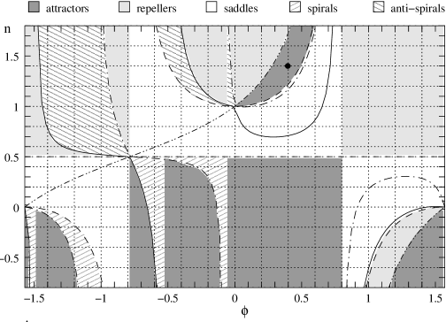
Figure 6: Stability of the line of fixed points $\mathcal{L}_{\infty}$ for LRS Bianchi I with matter. Results are independent of $w$. The black dot represents the fixed point at $\phi=0.4$ for a model with $n=1.4$.

5.3 Evolution of the shear

The trace free Gauss Codazzi equation (27) can in general (i.e. for all points in the phase space) be represented in terms of the dynamical variables (31) as

$$\frac{\dot{\sigma}}{\sigma}=-{\textstyle{1\over 3}}(2+\Sigma+y+z)\Theta.$$ (87)

The shear evolves at the same rate as in GR when $\dot{\sigma}/\sigma=-\Theta$, which holds for all values on the plane $1=\Sigma+y+z$. The shear will dissipate faster than in GR when $\dot{\sigma}/\sigma<-\Theta$, that is all points that lie in the region $1>\Sigma+y+z$. We may again call this the fast shear dissipation (FSD) regime. The shear will dissipate slower than in GR when $\dot{\sigma}/\sigma>-\Theta$ and hence all points in the region $1<\Sigma+y+z$. This will be called the slow shear dissipation (SSD) regime. Analysing the three dimensional phase space for this system is more difficult than the two dimensional spaces considered in the vacuum case since it is harder to visualise.

All the finite fixed points ($\mathcal{A}$, $\mathcal{B}$ and $\mathcal{C}$) together with the point $\Sigma_{*}=0$ on $\mathcal{L}_{1}$, lie on the plane $\Sigma=0$ and are therefore isotropic.

The evolution of the shear for the anisotropic fixed points on $\mathcal{L}_{1}$ can be obtained as in the vacuum case. For these points (87) take the form

$$\frac{\dot{\sigma}}{\sigma}=-{\textstyle{1\over 3}}(2+\Sigma_{*})\Theta=-(2+\Sigma_{*})\left(\frac{\dot{a}}{a}\right).$$ (88)

which may be integrated to give

$$\sigma=\sigma_{0}a^{-(2+\Sigma_{*})}=\sigma_{0}a_{0}^{-(2+\Sigma_{*})}(t-t_{0})^{-1},$$ (89)

where we made use of (38). This is the same solutions that where obtained in the vacuum case. This is to be expected since all these fixed points lie on the line $\mathcal{L}_{1}$ for which $z=0$.

The point $\mathcal{C}_{\infty}$ and the points on the line $\mathcal{L}_{\infty}$ (including $\mathcal{F}_{\infty}$) are the only asymptotic fixed points with non-vanishing shear. Point $\mathcal{C}_{\infty}$ lies on the line $\mathcal{L}_{1}$ and therefore has the solution

$$\sigma=\sigma_{0}a^{-(2+\Sigma_{c})}.$$ (90)

The behaviour of the shear for the fixed points on $\mathcal{L}_{\infty}$ can be found like (74), i.e by transforming (87) into polar coordinates and taking the limit $r\to 1$. The resulting equation then yields the solution $\sigma=\sigma_{0}={\rm constant}$.

6 Discussion and Conclusions

We have derived the evolution equations of the shear for Bianchi I cosmologies with $f(R)$-gravity. This general expression, allows us to consider the shear evolution for any function of the scalar curvature. However, because the shear depend non-linearly on the Ricci scalar one can not determine how the dissipation of the shear anisotropy compares with the case in GR even if one chooses a specific form for $f(R)$ (such as $R+R^{2}$ or $R^{n}$). One way of dealing with this problem is to make certain assumptions (for example the form of the evolution of the scale factor $a$ [9]) to obtain a solution. A more general approach is to make use of the dynamical systems approach to study HOTG in these cosmologies since it provides both exact solutions and the global behaviour of the system.

Our main aim in this paper was to see how the shear behaves in LRS Bianchi I cosmologies with $R^{n}$- gravity and whether these models isotropises at early and late times. To achieve this goal we used the theory of dynamical systems to analyse the system of equations governing the evolution of this model with and without matter.

The phase space for these models have a number of interesting features, in particular it contains one isotropic fixed point and a line of fixed points with non-vanishing shear. The isotropic fixed point is an attractor (stable node) for values of the parameter $n$ in the ranges $n<1/2$, $1/2<n<1$ and $n>5/4$. In the range $1<n<5/4$ this point is a repeller (unstable node) and therefore may be seen as a past attractor. An isotropic past attractor implies that inflation can start without requiring special initials conditions. However, since we have attractors for $(\sigma/H)_{*}<<1$ on $\mathcal{L}_{1}$, we may not need inflation since the shear anisotropy approaches a constant value which may be chosen as the expansion normalised shear observed today ($(\sigma/H)_{*}<10^{-9}$ [26, 27, 28]), provided that other observational constraints such as nucleosynthesis are satisfied.

We also found that the line $y=1-\Sigma$ separates the phase space into two part. For all points on this line, the shear dissipates at the same rate as in GR. In the region above the line the shear dissipates faster (FSD) than GR and in the region below the line, slower (SSD) than in GR. From Figures $1-5$ we can see that there are a number of orbits which cross the dotted line. These are systems which initially lie in the FSD region and then make a transition to the SSD region and vice versa. An interesting feature of the vacuum case is that when the evolution of the universe reaches the stable solutions on $\mathcal{L}_{1}$, the shear will evolve according to $\sigma\propto t^{-1}$ irrespective of the value of $n$. For values that lie in the range $1/2<n<1$ and $y>0$, one may have orbits that initially lie in the FSD region (see Figures 1 and 2) and then make a transition to the SSD region at late times. The opposite will happen for values that lie in the range $1<n<5/4$ and $y>0$. Initially the orbits lie in the SSD region (see Figure 3) and then make a transition to the FSD region.

We observe the same kind of behaviour in the matter case where the phase space is however 3-dimensional, but is similarly divided into two regions, by the plane $1=\Sigma+y+z$. The space above the plane is the SSD region and below the FSD region. Similar argument to the vacuum case can be used here to investigate the orbits. When matter is included we do however only have stable fixed points on $\mathcal{L}_{1}$ for values of $n$ in the range $1<n<5/4$.

In conclusion we have shown that $R^{n}$- gravity modifies the dynamics of the shear in LRS Bianchi I cosmologies by altering the rate at which the shear dissipates. There are cases in which the shear always dissipate slower or faster than in GR, and there are ones which make transitions from first evolving faster and later slower (and vice versa) than in GR.

References

References

- [1] Carroll S M, Duvvuri V, Trodden M and Turner M S 2004 Phys. Rev. D70 043528
- [2] Nojiri S and Odintsov S D 2003 Phys. Rev. D68 123512
- [3] Olmo G J 2005 Phys. Rev. D72 083505
- [4] Capozziello S 2002 Int. Journ. Mod. Phys. D 11 483
- [5] Capozziello S, Carloni S and Troisi A 2003 Recent Res. Devel. Astronomy & Astrophysics 1 625 (Preprint astro-ph/0303041)
- [6] Wainwright J and Ellis G F R (ed) 1997 Dynamical systems in cosmology (Cambridge: Cambridge University Press) (see also references therein)
- [7] Carloni S, Dunsby P K S, Capozziello S and Troisi A 2005 Class. Quantum Grav. 22 4839
- [8] Clifton T and Barrow J D 2005 Phys. Rev. D72 103005
- [9] Maartens R and Taylor D R 1994 Gen. Rel. Grav. 26 599
- [10] Ellis G F R 1973 Cargèse Lectures in Physics, Vol 6 (ed) E Scatzman (New York: Gordon and Breach)
- [11] Ellis G F R and van Elst H 1999 Cosmological Models (Cargèse Lectures 1998), Theoretical and Observational Cosmology (ed) M. Lachièze-Rey (Kluwer, Dordrecht) 1-116 (Preprint gr-qc/9812046)
- [12] Kasner E 1925 Trans. Am. Math. Soc. 27 101
- [13] Barrow J D and Clifton T 2006 Class. Quantum Grav. 23 L1
- [14] Clifton T and Barrow J D 2006 Class. Quantum Grav. 23 2951
- [15] Ellis G F R 1967 J. Math. Phys. 8 1171
- [16] Stewart J M and Ellis G F R 1968 J. Math. Phys. 9 1072
- [17] van Elst H and Ellis G F R 1996 Class. Quantum Grav. 13 1099
- [18] Coley A A 2002 Class. Quantum Grav. 19 L45
- [19] Coley A A 2002 Phys. Rev. D66 023512
- [20] Dunsby P K S, Goheer N, Bruni M and Coley A 2004 Phys. Rev. D69 101303
- [21] Goheer N, Dunsby P K S, Bruni M and Coley A 2004 Phys. Rev. D70 123517
- [22] Rippl S, van Elst H, Tavakol R and Taylor D 1996 Gen. Rel. Grav. 28 193
- [23] Berkin A L 1990 Phys. Rev. D42 1016
- [24] Holden D J and Wands D 1998 Class. Quantum Grav. 15 3271
- [25] Goode S W and Wainwright J 1985 Class. Quantum Grav. 2 99
- [26] Bunn E F, Ferreira P G and Silk J 1996 Phys. Rev. Lett. 77 2883
- [27] Kogut A, Hinshaw G and Banday A J 1997 Phys. Rev. D55 1901
- [28] Jaffe T R, Banday A J, Eriksen H K, Górski K M a nd Hansen F K 2005 Astrophys. J. 629 L1
- [29] Collins C B and Hawking S W 1973 Astrophys. J. 180 317
- [30] Strogatz S H 1994 Nonlinear Dynamics and Chaos (Cambridge, Massachusetts: Perseus Books)