On the Exact Solutions of the Regge-Wheeler Equation in the Schwarzschild Black Hole Interior

Abstract

We solve the Regge-Wheeler equation for axial perturbations of the Schwarzschild metric in the black hole interior in terms of Heun’s functions and give a description of the spectrum and the eigenfunctions of the interior problem. The phenomenon of attraction and repulsion of the discrete eigenvalues of gravitational waves is discovered.

Keywords: Schwarzschild black hole, gravitational waves, Regge-Wheeler equation, Heun’s functions.

PACS: 04.70.Bw, 04.30.-w., 04.30 Nx

1 Introduction

The perturbations of the gravitational field of black holes (BH) is a very active and large area of analytical, numerical, experimental and astrophysical research. Ongoing and future experiments, based on perturbation analysis and numerical calculations, are expected to give critical tests of the existing theories of gravity [1, 2]. For the experimental study of the gravitational waves a unprecedented precision of the already existing and future detectors must be reached [1, 2]. Since this is an extremely arduous and expensive task, an important goal of the theory is to reach detailed description of all features of the studied phenomena.

For the study of the perturbations outside the BH horizon one uses the quasi-normal modes (QNM) with well known complex spectra [3]. QNM do not form a complete basis of functions in the space of the linear metric’s perturbations. Nevertheless, they are widely used as a tool for theoretical study of the perturbations in the outer domain of BH. The QNM are believed to be relevant to the quantum gravity, too [4].

Analogous tool for the study of perturbations of the black hole interior is not known even in the simplest case of Schwarzschild black holes (SBH). Since the BH-spacetimes are considered to describe uniform physical objects with their exterior and interior, separated by an event horizon, it is natural to study the perturbations of the gravitational field in both domains, at least by reason of completeness.

In the classical theory of BH it seems reasonable to exclude from the most of the considerations the inner domain, because it does not influence directly the observable outer domain. Nevertheless, the excitations of degrees of freedom in the inner domain may be essential for the consideration of the total BH entropy and for construction of the quantum theory of BH. The interior excitations may yield observable effects in the exterior of the BH, due to the quantum effects, see, for example, the recent article [5] and references therein. To discuss such problems one needs a proper mathematical description of the BH-interior’s perturbations.

Another reason to study the BH interior was discovered in the very recent article [6]: It was shown that without excision of the inner domain around the singularity one can improve dramatically the long-term stability of the numerical calculations. Although the region of the space-time that is causally disconnected can be ignored for signals and perturbations traveling at physical speeds, numerical signals, such as gauge waves or constraint violations, may travel at velocities larger then that of light and thus leave the physically disconnected region.

Thus the study of the perturbations of the BH interior becomes an important issue both from analytical and numerical point of view.

In the present article we are starting the analytical and numerical investigation of the mathematical problem, introducing a large set of solutions for description of the perturbation of the SBH interior and studying the basic properties of the corresponding functions. We believe that this will help a more deep understanding of the problems of BH physics.

We show that one can find some unexpected new results for the perturbations of the SBH interior. In particular, we have discovered that variations of the boundary conditions at the event horizon $r=1$ produce attraction and repulsion of the discrete spectral levels of the gravitational waves in the SBH interior.

2 General Consideration of the Interior Problem

The proper mathematical ground for the investigation of the problem is the Regge-Wheeler equation (RWE) [7]:

$$\partial_{t}^{2}\Phi_{s,l}+\left(-\partial^{2}_{x}+V_{s,l}\right)\Phi_{s,l}=0.$$ (2.1)

Its study has a long history as well as important and significant achievements [3, 7].

The RWE describes the axial perturbations of the Schwarzschild metric of mass $M$ in the first order linear approximation. In Eq. (2.1) $x\!=\!r\!+\!r_{\!{}_{Sch}}\ln\left(|r/r_{\!{}_{Sch}}\!-\!1|\right)$ denotes the Regge-Wheeler ”tortoise” coordinate, $r_{\!{}_{Sch}}=2M$ is the Schwarzschild radius and $\Phi_{s,l}(t,r)$ is the radial function for perturbations of spin $s$ and angular momentum $l\!\geq\!s$. Hereafter we use units $r_{\!{}_{Sch}}\!=\!2M\!=\!1$. The effective potential in RWE (2.1) reads

$$V_{s,l}(r)=\left(1-{{1}\over r}\right)\left({{l(l+1)}\over{r^{2}}}+{{1-s^{2}}\over{r^{3}}}\right).$$

For $r\in[0,1]$ the area radius $r$ in it can be expressed explicitly as a function of the variable $x$ using Lambert W-function [8]: $r=W(-e^{x-1})+1$.

The most important case $s\!=\!2$ describes the gravitational waves and is our main subject here.

The standard ansatz $\Phi_{s,l}(t,r)=R_{\varepsilon,s,l}(r)e^{i\varepsilon t}$ brings us to the stationary problem in the outer domain $r>1$:

$$\partial^{2}_{x}R_{\varepsilon,s,l}+\left(\varepsilon^{2}-V_{s,l}\right)R_{\varepsilon,s,l}=0.$$ (2.2)

Its exact solutions were described recently [9] in terms of the confluent Heun’s functions $HeunC\!\left(\alpha,\beta,\gamma,\delta,\eta,r\right)$ [10].

Here we introduce for the first time the exact solutions of the Regge-Wheeler equation in the interior of the SBH. It is well known [11] that because of the change of the signs of the components $g_{tt}=-1/g_{rr}=1-1/r$ of the metric, in this domain the former Schwarzschild-time variable $t$ plays the role of radial space variable $r_{in}=t\in(0,\infty)$ and the area radius $r\in(1,0)$, plays the role of time variable. As a result, the Regge-Wheeler ”tortoise” coordinate $x\in(-\infty,0)$ presents a specific time coordinate in the inner domain. For the study of the solutions of Eq. (2.1) in this domain it is useful to stretch the last interval to the standard one by a further change of the time-variable: $x\to t_{in}=x-1/x\in(-\infty,\infty)$.

These notes are important for the physical interpretation of the mathematical results. In particular, it is natural to write down the interior solutions of the RWE in the form: $\Phi_{\varepsilon,s,l}^{in}(r_{in},t_{in})=e^{i\varepsilon r_{in}}R_{\varepsilon,s,l}\left(r(t_{in})\right)$, where

$$r(t_{in})\!=\!W\!\left(-exp\left({{t_{in}}\over{2}}\!-\!1\!-\!\sqrt{\left({{t_{in}}\over{2}}\right)^{2}\!+\!1}\,\right)\right)\!\!+\!1.\hskip 8.5359pt$$ (2.3)

The dependence of this solution on the interior radial variable $r_{in}$ is simple. Its dependence on the interior time $t_{in}$ is governed by the RWE (2.2) with interior-time-dependent potential $V_{s,l}$. In despite of this unusual feature of the solutions in the SBH interior, this way we obtain a basis of functions, which are suitable for the study of the corresponding linear perturbations.

Without any additional conditions the differential equation (2.2) has a reach variety of solutions which may describe different physical problems. For a correct formulation of a given physical problem one must restrict the class of the solutions using proper boundary conditions. Since the physics at the boundary influences strongly the solutions of the problem, the boundary conditions are a necessary ingredient of the theory and define the physical problem under consideration.

The solutions of the Eq. (2.2), which are not regular at the point $r=0$ are not stable, since they grow up infinitely as $t_{in}\!\to\!+\infty$. In addition they have a complicated series expansion with logarithmic terms [10]. Hence, these solutions are not single-valued functions and have no suitable properties for physical applications.

Solutions of the Eq. (2.2), which grow up infinitely with respect to the future direction of the exterior time $t$ exist in the exterior domain of SBH, too. They are physically unacceptable and therefore are excluded by formulation of a proper boundary problem [3, 7]. Only after that the physical problem is fixed and one can prove the stability of the remaining solutions (QNM) and small perturbations of general form with respect to the exterior-time evolution [12]. All these solutions unavoidably grow up infinitely both at the space infinity and at the horizon [3, 7, 9].

By analogy with the consideration in the outer domain of SBH, in the inner one we are considering only the solutions, which are stable with respect to the future direction of the interior time. Indeed, the common physical sense states that only the stable solutions are of physical interest. Therefore in this article we study the solutions, which are regular at the point $r\!=\!0$, formulating the corresponding boundary problem. The remaining solutions are stable in the future direction of the interior time: $t_{in}\!\to\!+\infty$ and have a nontrivial spectrum with novel properties.

From a pure mathematical point of view in the present article we are considering the two-singular-points-boundary problem [10, 9] for the RWE on the interval $r\in[0,1]$. In this sense here we present an extension of the article [9], where only exact solutions of different types on the intervals $r\in[0,\infty)$ and $r\in[r_{*},\infty)\subset[0,\infty)$ were studied in detail.

There exist one more possibility: to study two-singular-points-boundary problem for the Eq. (2.2) on the interval $r\in[0,\infty)$ using some contour in the complex plane ${\cal C}_{r}$ with singular ends $0\,\,\hbox{and}\,\,\infty$, which turns round on the third singular point $r=1$. Such solutions may describe mutual perturbations both of SBH exterior and interior. This interesting possibility seems to correspond to the perturbations of the Kruscal-Szekeres extension of the Schwarzschild solution [11]. It is beyond the scope of the present article and will be considered somewhere else.

3 The Exact Solutions in the SBH interior

The RWE (2.2) has three singular points: the origin $r\!=\!0$, the horizon $r\!=\!1$ and the infinite point $r\!=\!\infty$. The first two are regular singular points and can be treated on equal terms. The last one is an irregular singular point, obtained by confluence of two regular singular points in the general Heun’s equation. As a result, in the interior of the SBH around the regular singular points we have the following local analytical solutions [9]:

$$R_{\,\,\varepsilon,s,l}^{(0)-}(r)=r^{s+1}e^{i\varepsilon\left(\ln(1-r)+r\right)}HeunC\!\left(2i\varepsilon,2s,2i\varepsilon,2\varepsilon^{2},s^{2}-l(l+1),r\right),$$ (3.1)

$$R_{\,\,\varepsilon,s,l}^{(1)\pm}(r)\!=\!r^{s\!+\!1}e^{\!\pm i\varepsilon\left(\ln(1\!-\!r)\!-r\right)}HeunC\!\left(\pm 2i\varepsilon,\pm 2i\varepsilon,2s,-2\varepsilon^{2},2\varepsilon^{2}\!\!+\!s^{2}\!\!-\!l(l\!+\!1),1\!-\!r\right)\!.\hskip 11.38092pt$$ (3.2)

The solution (3.1) is the only one, which is regular at the point $r=0$. In addition it is the only single-valued local solution, defined around this point.

The solution $R_{\,\,\varepsilon,s,l}^{(1)+}(r)$ in (3.2) can be derived from the one, used in [9], applying proper transformations of the Heun’s functions [10]. For $\varepsilon\neq 0$ the functions $R_{\,\,\varepsilon,s,l}^{(1)\pm}(r)$ (3.2) define a pair of linearly independent solutions with the symmetry property

$$R_{\,\,\varepsilon,s,l}^{(1)\pm}(r)=R_{\,\,-\varepsilon,s,l}^{(1)\mp}(r).$$ (3.3)

4 The Interior Spectral Problem

4.1 The Continuous Spectrum ($\varepsilon^{2}>0$).

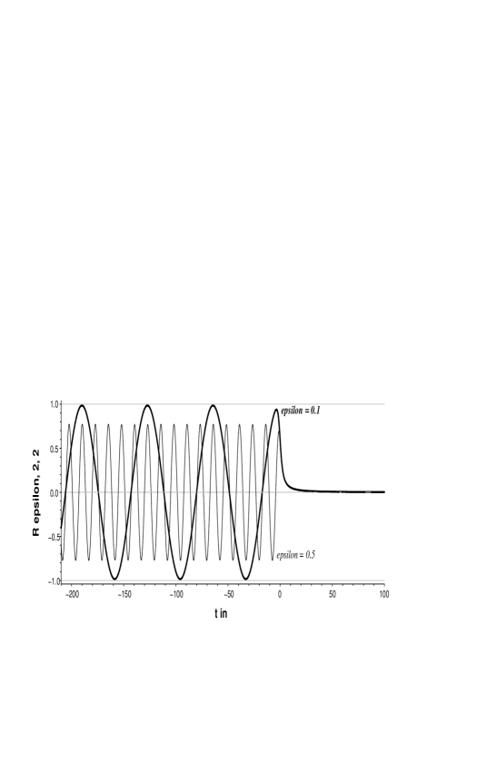
Figure 1: Two solutions of the continuous spectrum.

For real $\varepsilon^{2}>0$ the problem has a real continuous spectrum. The corresponding solutions $R_{\varepsilon,2,2}(t_{in})$ are illustrated in Fig. 1. They define a basis of stable normal modes for perturbations of the metric in the SBH interior and can be used for Fourier expansion of perturbations of more general form.

As seen in the Fig. 1, the use of the inner time variable $t_{in}$ instead of the tortoise coordinate $x$ makes the variations of the solutions almost equidistant in the limit $t_{in}\to-\infty$. This property makes the inner time variable $t_{in}$ to seem the most natural one in the SBH interior. Using variables like $r$ or $x$ we lose this property and meet numerical problems in this limit.

4.2 The Special Solutions with $\varepsilon^{2}=0$.

The zero eigenvalue $\varepsilon=0$ yields a degenerate case in which the two functions (3.2) coincide. Then we obtain the infinite series of polynomial solutions:

$$R_{\,\,\varepsilon=0,s,l}^{(0)-}(r)\!=\!{{(l\!-\!s)!}\over{Poch(1\!+\!2s,l\!-\!s)}}r^{s\!+\!1}JacobiP(l\!-\!s,2s,0,1\!-\!2r)=r^{3}\!+\!\dots,$$ (4.1)

which are finite on the whole interval $r\in[0,1]$. These functions form an orthogonal basis with respect to the measure $w(r)=(1-r)^{2s}$. Here $JacobiP(n,a,b,z)$ stands for the standard Jacobi polynomials and $Poch(c,d)$ – for the Pochhammer symbol.

The basis of the stable normal modes (4.1) is suitable for series expansion of the perturbations of $\varepsilon=0$. These solutions do not depend on the variable $r_{in}$ and are the only ones, which are finite at both singular ends of the interval $r\in[0,1]$.

4.3 The Discrete Spectrum ($\varepsilon^{2}<0$).

The discrete spectrum of the problem at hand corresponds to pure imaginary values of the parameter $\varepsilon$, i.e. to Laplace transform of the perturbations of general form, instead of their Fourier transform, which corresponds to real values of $\varepsilon$. Thus, studying the the case $\varepsilon^{2}<0$ we are constructing a basis for Laplace expansion of the perturbations of more general form in the SBH interior.

For a qualitative analysis of the discrete spectrum we can apply the Ferrari-Mashhoon transformation [13]: $x\to\tilde{x}=-ix$, $r_{s}\to\tilde{r}_{s}=-ir_{s}$, $V\to\tilde{V}=-V$. It reduces our spectral problem to a standard one: to find the bound states in the inverted potential $\tilde{V}$. For $s\geq 2$ the latter describes two negative-valued potential wells i) a finite one, in which one may have several negative eigenvalues, and ii) an infinite one, in which one has infinite series of negative eigenvalues. In both cases $\varepsilon^{2}\leq 0$. Hence, $Re\left(\varepsilon\right)\equiv 0$. Then the functions (3.1), (3.2) and all their parameters are real. In particular,

$$R_{\,\,\varepsilon,s,l}^{(0)-}(r)\!=\!\Gamma_{1+}^{0-}(\varepsilon,s,l)R_{\,\,\varepsilon,s,l}^{(1)+}(r)+\Gamma_{1-}^{0-}(\varepsilon,s,l)R_{\,\,\varepsilon,s,l}^{(1)-}(r)$$ (4.2)

$$\hskip 46.94687pt\sim\cos\alpha\,R_{\,\,\varepsilon,s,l}^{(1)+}(r)+\sin\alpha\,R_{\,\,\varepsilon,s,l}^{(1)-}(r)\hskip 56.9055pt$$

with real transition coefficients $\Gamma_{1-}^{0\pm}$ [9] and real mixing angle $\alpha$:

$$\tan\alpha=\Gamma_{1-}^{0-}(\varepsilon,s,l)/\Gamma_{1+}^{0-}(\varepsilon,s,l)\in\mathbb{R},\,\,\,\hbox{for}\,\,\,\varepsilon=i\varepsilon_{I}.\hskip 8.5359pt$$ (4.3)

The physical meaning of the mixing angle $\alpha$ is obvious: since the solutions $R_{\,\,\varepsilon,s,l}^{(1)+}(r)$ describe the ingoing into the horizon waves and the solutions $R_{\,\,\varepsilon,s,l}^{(1)-}(r)$ – the outgoing from the horizon waves [9], this angle describes the ratio of the amplitudes of these waves in their mixture (4.2). The value $\alpha=0$ corresponds to absence of the outgoing waves, and the value $\alpha=\pi/2$ describes the case without ingoing waves. Thus, fixing the value of the mixing angle $\alpha$ we are defining completely the physical problem under consideration.

When $r\to 0$, the asymptotic of the inverted potential is $\tilde{V}\sim(1-s^{2})r^{-4}$. Hence, we arrive at the well known from quantum mechanics specific physical problem of ”falling at the centrum” – the singular point $r=0$. Mathematically this means that the corresponding differential operator on the interval $r\in[0,1]$ has a defect [14] and we need an additional physical conditions to fix the eigenvalue problem. In our case such conditions are the regularity condition of solutions at the singular point $r=0$ and the fixation of the mixing angle $\alpha$, i.e. the justification of the physical conditions at the second singular point – the horizon $r=1$. Thus, for any given value of $\alpha$ the Eq. (4.3) presents a specific spectral equation for the eigenvalues.

Unfortunately, at present the transition coefficients $\Gamma_{1\pm}^{0-}(\varepsilon,s,l)$ are not known explicitly [10]. Therefore we replace the spectral equation (4.3) with the equivalent one:

$$\left|\begin{array}[]{cc}R_{\,\,\varepsilon,s,l}^{(0)-}(r_{1})&\cos\alpha\,R_{\,\,\varepsilon,s,l}^{(1)+}(r_{1})\!+\!\sin\alpha\,R_{\,\,\varepsilon,s,l}^{(1)-}(r_{1})\\ R_{\,\,\varepsilon,s,l}^{(0)-}(r_{2})&\cos\alpha\,R_{\,\,\varepsilon,s,l}^{(1)+}(r_{2})\!+\!\sin\alpha\,R_{\,\,\varepsilon,s,l}^{(1)-}(r_{2})\end{array}\right|=0,\hskip 17.07182pt$$ (4.6)

where $r_{1,2}\in(0,1),r_{1}\neq r_{2}$ are two otherwise arbitrary points. Because of the symmetry property (3.3), it is enough to study only the solutions $\varepsilon_{n,s,l}$ of the equation (4.6) with positive $\varepsilon_{I}=Im\left(\varepsilon_{n,s,l}\right)>0$.

We apply the complex plot abilities of Maple 10 to find a relatively small vicinity of the complex roots of this equation and then we justify their values by Muller’s method for finding of complex roots [15]. Our numerical results for $Im\left(\varepsilon_{n,2,2}\right)$ are shown in the Table 1 and in Figs. 2–5.

$n$	$\Big{|}$ $Im\left(\varepsilon_{n,2,2}\right)$	$\Big{|}$ $n$	$\Big{|}$ $Im\left(\varepsilon_{n,2,2}\right)$	$\Big{|}$ $n$   $\Big{|}$ $Im\left(\varepsilon_{n,2,2}\right)$
$1$	$\Big{|}$ 0.7523	$\Big{|}$ $7$	$\Big{|}$ 4.5138	$\Big{|}$ $13$ $\Big{|}$ 7.5657
$2$	$\Big{|}$ 1.3463	$\Big{|}$ $8$	$\Big{|}$ 5.0256	$\Big{|}$ $14$ $\Big{|}$ 8.0714
$3$	$\Big{|}$ 1.8999	$\Big{|}$ $9$	$\Big{|}$ 5.5357	$\Big{|}$ $15$ $\Big{|}$ 8.5768
$4$	$\Big{|}$ 2.4361	$\Big{|}$ $10$	$\Big{|}$ 6.0446	$\Big{|}$ $16$ $\Big{|}$ 9.0823
$5$	$\Big{|}$ 2.9627	$\Big{|}$ $11$	$\Big{|}$ 6.5524	$\Big{|}$ $17$ $\Big{|}$ 9.5867
$6$	$\Big{|}$ 3.4833	$\Big{|}$ $12$	$\Big{|}$ 7.0594	$\Big{|}$ $18$ $\Big{|}$ 10.0939

Table 1: The values of the first 18 eigenvalues of the RWE for SBH interior for $s=l=2$ and $\alpha=0$.

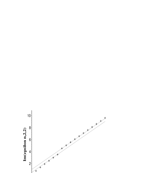
Figure 2: The first 18 eigenvalues (for $s=l=2$ and $\alpha=0$).

In the Fig.2 we see the first 18 eigenvalues (including the zero eigenvalue) of the RWE for SBH interior for $s=l=2$ and $\alpha=0$. The two series: $n=0,1,\dots 6$; and $n=7,\dots$ are clearly seen. They are placed around the straight lines $\varepsilon_{I}=n/2+1/2$ and $\varepsilon_{I}=n/2+1$, correspondingly.

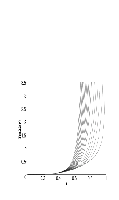
Figure 3: From right to the left: The first 18 eigenfunctions (for n=1, 2,…,18, s=l=2 and $\alpha=0$).          

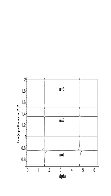
Figure 4: The dependence of $Im\left(\varepsilon_{n,2,2}\right)$ on the mixing angle $\alpha\in[0,2\pi]$.          

In Fig.4 we see a specific attraction and repulsion of the eigenvalues $\varepsilon_{n,s,l}(\alpha)$. Such behavior is typical for the eigenvalue problems related with the Heun’s equation [10]. It is well known in the quantum physics. To the best of our knowledge, this phenomenon is observed for the first time in the theory of SBH. Several additional remarks are in order:

1. Solving Eq. (4.6) one is unable to obtain the eigenvalues $\varepsilon_{N/2,2,2}({\pi\over 2})=i{N\over 2},N\in\mathbb{Z}^{+}$, i.e., when $\alpha\!=\!{\pi\over 2}/\!\!\!\mod\pi$ (the small circles in Fig.4). A pure numerical study of the RWE (2.2) shows that in these cases the solutions have the same behavior as the one, demonstated in Fig.3. Hence, one has to be careful, taking the corresponding limits in the analytical expressions (3.1), (3.2).

2. In the second series: $n=7,...$ the dependence of the eigenvalues on the mixing angle is similar to the one, shown in Fig.4, but $Im\left(\varepsilon_{n,2,2}\right)$ are decreasing functions of $\alpha$. The amplitudes of their variations are extremely small ($<10^{-9}$) and they are practically constant on the larger part of the interval $\alpha\in[0,2\pi]$.

3. There exist two more series of eigenvalues $\varepsilon_{n,2,2}$. For them all $Im\left(\varepsilon_{n,2,2}\right)$ are negative. These have the same absolute values as the eigenvalues, shown in Table 1 and in Fig.4. Their dependence on the mixing angle $\alpha$ is shifted by ${\pi\over 2}$ and correspondingly inverted. Because of this shift, the behavior of the corresponding eigenfunctions is the same as the one, demonstrated in Fig.3. This reflects the symmetry property (3.3) of the solutions.

4. The behavior of the eigenfunctions $R_{1,2,l}(r)$ with $l=3,\dots$ is the same as of the functions $R_{1,2,1}(r)$ in Fig.3. The dependence of the eigenvalues $\varepsilon_{1,2,l}(\alpha=0)$ on the angular momentum $l$ is shown in Fig.5.

5. The eigenfunctions $R_{n,2,l}(r)$ with $n>1,l>2$ start from infinity at $r=1$ and approach zero at $r=0$, oscillating around the zero value. The number of oscillations depends on the numbers $n$ and $l$.

Figure 5:   The dependence of the eigenvalues $\varepsilon_{1,2,l}(\alpha=0)$ on the angular momentum $l$.          

6. Our results bring to light a complementary information about the stability problem of SBH. Up to now only the stability of the exterior domain has been studied in linear approximation [12]. Here we have found the following details about stability properties of the solutions in the SBH interior:

$\bullet$ As we see in Figs. 1, 3, all solutions of Eq. (2.1), which are considered in the present article, are stable in direction of the interior-time-future ($t_{in}\to+\infty$), according to Lyapunov criterion. If $\varepsilon\neq 0$, these solutions are unstable in direction of the interior-time-past ($t_{in}\to-\infty$) according to Lyapunov criterion.

$\bullet$ There is a basic difference in the stability properties of the solutions of continuous spectrum (real $\varepsilon,\,\,\,\varepsilon^{2}>0$), which are of limited variation when $t_{in}\to-\infty$ and thus – stable in direction of the interior-time past in this weaker sense, and the solutions of discrete spectrum (imaginary $\varepsilon,\,\,\,\varepsilon^{2}<0$), which grow up infinitely when $t_{in}\to-\infty$ and, hence, are unstable in this direction of the interior time in any sense.

$\bullet$ All other interior solutions of the Regge-Wheeler equation with $\varepsilon\neq 0$, which are not considered in this article, are unstable in the future direction of the interior time and drop out of the physical consideration.

$\bullet$ There do not exist interior solutions, different from the above ones with $\varepsilon=0$ (see Eq. (4.1)), which are stable in both directions of the interior time.

5 Concluding Remarks

In this article we have shown that the Heun’s functions are an adequate powerful tool for description of the linear perturbations of the gravitational field not only outside the SBH horizon [9], but in their interior domain as well.

It is well known that every analytical function is defined completely by its singularities in the whole compactified complex domain. In the previous investigations of the specific properties of the solutions of RWE was used only the structure of these singular points, see the review articles [3] and the huge amount of reverences therein. Using many different mathematical technics, this way were reached important results for perturbations in the exterior of SBH. Some of the used methods of that type may be not applicable for the study of perturbations in the SBH interior.

Here we overcome the limits of that methods, using directly the properties of Heun’s functions, see for example Eq. (3.1), (3.2), (3.3), (4.3), etc. and writing down the corresponding explicit analytical solutions of the RWE.

All numerical results were obtained using Maple 10 package for performing direct calculations with these functions. Owing to the new version 10 of the Maple package, at present we are able to work with the Heun’s functions in the complex domain, thus obtaining a new freedom and new tools for the study of different new boundary problems for RWE, as well as for study of the old ones, applying new technics.

Using Heun’s functions we have obtained the analytical and the numerical description of all solutions of the Regge-Wheeler equation in the SBH interior, which are stable in direction of the interior-time future and single-valued functions in the whole complex domain. Having in our disposal these solutions we are ready for a more deep understanding of the problems of BH physics.

For example, as we have seen, the perturbations of SBH metric do not change the singularity at the point $r=0$, at least in the first order of perturbation theory. This result can be used for further justification of the numerical treatment of BH problems without excision of the interior domain. Now it becomes clear, that due to the unavoidable numerical errors in the interior of the BH one will lose the small stable single-valued physical solution around the point $r=0$ at the background of the big nonphysical solution. Hence, in order to obtain physically correct and stable numerical results one must suppress by proper techniques this nonphysical solution.

We have shown that under proper boundary conditions there exist interior solutions both of real continuous spectrum and of pure imaginary discrete spectrum. The first may form a basis for Fourier transform of linear perturbations of general form in SBH interior. The second may form analogous basis for Laplace transform. The investigation of the completeness of these sets of functions as a basis for the corresponding expansions and the analytical proof of the numerical results of the present article remain an open problem.

Our numerical study shows that there do not exist other solutions of the spectral equation (4.6). In particular, in the two-singular-points-boundary problem on the interval $r\in[0,1]$ we do not found solutions with $Re(\varepsilon)\times Im(\varepsilon)\neq 0$, in contrast to the case of exterior domain perturbations of SBH.

The discrete pure imaginary eigenvalues have a nontrivial behavior under changes of the boundary conditions at the horizon, described by the mixing angle $\alpha$. The phenomenon of attraction and repulsion of these eigenvalues has been observed.

The basic properties of the considered solutions have been studied and a new information about stability of the solutions of RWE in the SBH interior was obtained.

In the present article we have studied only the most important from physical point of view perturbations of SBH with $s=2$. The detailed study of the solutions with $s=0,1$ may be useful for numerical relativity in the spirit of the article [6].

Acknowledgments

The author is grateful to the High Energy Physics Division, ICTP, Trieste, for the hospitality and for the nice working conditions during his visit in the autumn of 2003. There the idea of the present article was created. The author is grateful to the JINR, Dubna, too, for the priority financial support of a cycle of scientific researches and for the hospitality and the good working conditions during his three months visits in 2003, 2004 and 2005. This article also was supported by the Scientific Found of Sofia University, Contract 70/2006, by its Foundation ”Theoretical and Computational Physics and Astrophysics” and by the Scientific Found of the Bulgarian Ministry of Sciences and Education, Contract VUF 06/05.

The author is thankful to Nikolay Vitaniov for the reading of the manuscript and the useful suggestions, to Luciano Rezzolla for the useful and stimulating discussion of the results of the present article and their relation with the recently found numerical techniques for treatment of BH problems without excision of the interior domain, and to Kostas Kokkotas for discussion of the exact solutions of RWE and SBH interior solutions during the XXIV Spanish Relativity Meeting, E.R.E. 2006.

References

- [1] Thorne K S 2003 Warping spacetime, in The Future of Theoretical Physics and Cosmology, Celebrating Stephen Hawking’s 60th Bird Day (Cambrige: Cambridge University Press)
- [2] Mours B and Marion F, ed Proceedings of the 9-th Gravitational Wave Data Analysis Workshop, Annecy, France, 15-18 December 2004, 2005 Class. Quant. Grav. 22 special issue
- [3] Ferrari V 1995 in Proc. of 7-th Marcel Grossmann Meeting ed R Ruffini and M Kaiser (Singapoore: World Scientific) Ferrari V 1998 in Black Holes and Relativistic Stars ed R Wald (Chikago: University Chicago Press) Kokkotas K D and Schmidt B G 1999 Living Rev. Relativity 2 2 Nollert H-P 1999 Class. Quant. Grav. 16 R159 Nagar A and Rezzola L 2005 Class. Quant. Grav. 22 R167
- [4] Motl L Adv. 2003 Theor. Math. Phys. 6 1135 Motl L and Neitzke A 2003 Adv. Theor. Math. Phys. 7 307 Berti E 2004 Black hole quasinormal modes: hints of quantum gravity? gr-qc/0411025. Natário J and Schiappa R 2004 Adv. Theor. Math. Phys. 8 1001-1131
- [5] Balasubramanian V, Marolf D and Rosali M 2006 Information recovery from black holes hep-th/0604045
- [6] Baiotti L and Rezzolla L 2006 Challenging the paradigm of singularity excision in gravitational collapse gr-qc/0608113
- [7] Regge T and Wheeler J A 1957 Phys. Rev. 108 1063 Chandrasekhar S 1983 The Mathematical Theory of Black Holes (Oxford: Oxford University Press)
- [8] Corless R M, Gonnet G H, Hare D E G, Jeffrey D. J and Knuth D E 1996 Advances in Comp. Math. 5 329
- [9] Fiziev P P 2006 Class. Qunt. Grav. 23 2447
- [10] Heun K 1889 Math. Ann. 33 161 Bateman H and Erdélyi A 1955 Higher Transcendental Functions, Vol. 3 (New York: Mc Grow-Hill) Decarreau A, Dumont-Lepage M Cl, Maroni P, Robert A and Roneaux A 1978 Ann. Soc. Buxelles 92 53 Decarreau A and Maroni P Robert A 1978 Ann. Soc. Buxelles 92 151 Decarreau A and Maroni P Robert A 1995 Heun’s Differential Equations ed. A Roneaux (Oxford: Oxford University Press) Slavyanov S Y and Lay W 2000 Special Functions, A Unified Theory Based on Singularities (Oxford Mathematical Monographs) (Oxford: Oxford University Press)
- [11] Landau L D and Lifshitz E M 1962 The Classical Theory of Fields 2d ed (Reading Mass: Addison-Wesley) Misner C, Thorne K S and Wheeler J A 1973 Gravity (W H Freemand & Co) Adler R, Bazin M and Schiffer M 1975 Introduction to General Relativity Sec. ed. (McFraw-Hill Co) Frolov V P and Novikov I D, 1998 Black Hole Physics (Kuwer Acad. Publ.) Rindler W 2001 Relativity (Oxford: Oxford University Press)
- [12] Vishveshwara C V 1970 Phys. Rev. D 1 2870 Steward J M 1975 Proc. R. Soc. A 344 65 Wald R M 1979 J. Math. Phys. 20 1056
- [13] Ferrari V and Mashhoon B 1984 Phys. Rev. D 30 295
- [14] Reed M and Simon B 1975 Methods of Modern Mathematical Physics Vol. II (New York: Acad. Press)
- [15] Press W H, Teukolsly S A, Wetterling W T and Flannery B P 1992 Numerical Recipes in Fortran 77 Vol. 1 Second Edition (Cambrige: Cambrige University Press)