Abstract

In part I we study quantum modified photon trajectories in a Schwarzschild blackhole spacetime. The photon vacuum polarization effect in curved spacetime leads to birefringence, i.e. the photon velocity becomes $c\pm\delta c$ depending on its polarization. This velocity shift then results in modified photon trajectories.

We find that photon trajectories are shifted by equal and opposite amounts for the two photon polarizations, as expected by the sum rule [5]. Therefore, the critical circular orbit at $u=1/3M$ in Schwarzschild spacetime, is split depending on polarization as $u=1/3M\pm A\delta(M)$ (to first order in $A$), where $A$ is a constant found to be $\sim 10^{-32}$ for a solar mass blackhole. Then using general quantum modified trajectory equations we find that photons projected into the blackhole for a critical impact parameter tend to the critical orbit associated with that polarization. We then use an impact parameter that is lower than the critical one. In this case the photons tend to the event horizon in coordinate time, and according to the affine parameter the photons fall into the singularity. This means even with the quantum corrections the event horizon behaves in the classic way, as expected from the horizon theorem [5].

We also construct a quantum modified Schwarzschild metric, which encompasses the quantum polarization corrections. This is then used to derive the photons general quantum modified equations of motion, as before. We also show that when this modified metric is used with wave vectors for radially projected photons we obtain the classic equations of motion, as expected, because radial velocities are not modified by the quantum polarization correction.

In Part II we use the 2+1d Nambu–Jona-Lasino (NJL) model to study the superfluid behaviour of two-dimensional quark matter. In previous work, [12], it was suggested that the high density phase of the 2+1d NJL model could be a relativistic gapless thin film BCS superfluid. In this work we find that as we raise the baryon chemical potential ($\mu$) the baryon supercurrent jumps from a non-superfluid (zero) phase to a superfluid (non-zero) phase. This sharp transition is seen to occur in the region $0.65<\mu_{c}<0.68$, which was shown in [12] to be the region of chiral symmetry restoration. In this analysis we prove that at high density the $2+1d$ NJL model is in a superfluid phase.

We then go on to study the dynamics of the superfluid phase, represented by the helicity modulus ($\Upsilon$ ), which is the constant of proportionality between the supercurrent and the gradient of the diquark state function. We find that below the temperature associated with lattice size $L_{t}=4$, the system is in a non-superfluid phase, and above $L_{t}=24$ the system is in a superfluid phase. We also find a possible 2nd order transition at $L_{t}\approx 6$, which corresponds to the critical point as described by Kosterlitz and Thouless’ theory of $2D$ critical systems with $U(1)$ global symmetry - such as the $XY$ model.

For my family

UNIVERSITY OF WALES SWANSEA

Author:                  Avtar Singh Sehra
Title:                      Particles Under Extreme Conditions
Department:           Department of Physics
Degree:                   Ph.D.
Year:                      2005



This work has not previously been accepted in substance for any degree and is not being concurrently submitted in candidature for any degree.

This thesis is the result of my own investigations, except where otherwise stated. Other sources are acknowledged by explicit references. A bibliography is appended.

I hereby give consent for my thesis, if accepted, to be available for photocopying and for inter-library loan, and for the title and summary to be made available to outside organisations.

Preface

In this work we will be dealing with quantum particles under extreme conditions. This will include the study of quantum modified photon trajectories in a highly curved background spacetime (Schwarzschild blackhole spacetime) and high density quark matter in two dimensional films.

Part 1: Quantum Modified Null Trajectories in Schwarzschild Spacetime

In this part we will be studying the quantum modifications to null geodesics in Schwarzschild spacetime, in particular the modifications to the critical stable orbit. In Chapter 1 we will give an introduction to the the vacuum polarization effect that leads to the modification of photon trajectories in general relativity. In Chapter 2 we will give an introduction to the derivation of the orbit equation in Schwarzschild spacetime, including the techniques involved in solving it and the interpretation of results, i.e. for critical stable orbits and trajectories to the singularity. In Chapter 3 we will then provide an introduction to the techniques of geometric optics, i.e. the derivation of the light-cone and geodesic equation from Maxwell’s equations of motion in curved spacetime (with and without the quantum corrections). We will also give a brief overview of previous theories associated with quantum modified null geodesics, such as the horizon theorem and the polarization sum rule. In Chapter 4 we will go onto using theses techniques in order to determine the quantum modified critical circular orbits, and the changes in the associated critical impact parameters. These finding will then be extended, by deriving a general quantum modified equation of motion. Using this, with the modified impact parameters, we will study the modifications to general null geodesics as they tend to the critical stable orbits. Also, using the quantum modified general equation of motion, we will show that a general geodesic aimed into the black hole behaves in the classical way around the event horizon, as described by the horizon theorem. In Chapter 5 we will encompass these results into a quantum modified Schwarzschild metric.

Part 2: Study of the 2+1d NJL Gapless Superfluid

In this part we will be studying high density quark matter in two dimensional films using the 2+1d Nambu-Jona-Lasino (NJL) model, in particular to isolate a critical gapless BCS superfluid phase, which was suspected to exist in [12]. In Chapter 7 we will set the scene for this work by giving an overview of quantum chromodynamics, its symmetries and aspects of its phase diagram. In Chapter 8 we will give a brief introduction to the NJL model; then we will go on to discuss the techniques and results of the previous simulations of the NJL model, given in 2+1d [12], i.e. simulation of the diquark condensate through the introduction of diquark sources, and the evidence of chiral symmetry restoration and the non-zero baryon density. In Chapter 9 we will extend the baryon density to a baryon three current by the use of Ward identities, these are then implemented into the simulation. We also introduce a spatially varying diquark source, referred to as a twisted source. In this way a gradient in the diquark pair wave function is introduced, which forces a flow of the baryon current, which will then be measured. We will then explore the behaviour of the 3-current (using the helicity modules, $\Upsilon$, Sec. 9.2) with variations in spatial volume, temperature, and variations in the diquark source, in order to isolate the superfluid (and non-superfluid) state of the 2+1d NJL model. In Chapter 10 we will study the variation of the helicity modulus with temperature; which will be done in order to determine the critical point of the system, i.e. the point where vortex and antivortex pairs come together to form the superfluid phase (as predicted in the condensed matter study of 2 dimensional systems, e.g. the XY model).

Contents

1. Abstract
2. Acknowledgments
3. Preface
4. I Quantum Modified Null Trajectories in Schwarzschild Spacetime
   1. 1 Introduction
      1. 1.1 General Relativity
      2. 1.2 QED in a Curved Spacetime
      3. 1.3 The Equivalence Principle and Causality
      4. 1.4 Critical Stable Orbits
   2. 2 Null Dynamics in Schwarzschild Spacetime
      1. 2.1 Equations of Motion
         1. 2.1.1 Orbit Equation
      2. 2.2 Orbits in Schwarzschild Spacetime
         1. 2.2.1 Null Radial Geodesic
         2. 2.2.2 General Null Geodesics and Critical Orbits
   3. 3 Quantum Gravitational Optics
      1. 3.1 Photon Propagation in Curved Spacetime
         1. 3.1.1 Geometric Optics in Curved Spacetime
      2. 3.2 Quantum Modified Null Dynamics
      3. 3.3 Horizon Theorem and Polarization Rule
         1. 3.3.1 Polarization Sum Rule
         2. 3.3.2 Horizon Theorem
   4. 4 Quantum Modified Trajectories
      1. 4.1 Quantum Modified Circular Orbits
         1. 4.1.1 Quantum Modified Critical Orbits
      2. 4.2 Quantum Modified General Geodesics
         1. 4.2.1 General Vectors
         2. 4.2.2 Quantum Modification
         3. 4.2.3 General Trajectory to the Critical Orbit.
      3. 4.3 Quantum Modification and the Event Horizon
         1. 4.3.1 Trajectories to the singularity
         2. 4.3.2 Fixed Event Horizon
   5. 5 Quantum Modified Schwarzschild Metric
      1. 5.1 Construction of the Metric
      2. 5.2 Dynamics with the Quantum Modified Metric
   6. 6 Summary
5. II Superfluid Behaviour of the 2+1d NJL Model at High Density
   1. 7 Introduction
      1. 7.1 Quantum Chromodynamics
         1. 7.1.1 QCD: A Model of Strongly Interacting Matter
         2. 7.1.2 Lattice QCD
      2. 7.2 Chiral Symmetry in QCD
         1. 7.2.1 Helicity and Chirality
         2. 7.2.2 Chiral Symmetry
         3. 7.2.3 The QCD Vacuum and Spontaneous Symmetry Breaking
      3. 7.3 The QCD Phase Diagram
         1. 7.3.1 A Classic Phase Diagram of $H_{2}O$
         2. 7.3.2 A Map of the QCD Phase Diagram
         3. 7.3.3 Restoration of Chiral Symmetry
      4. 7.4 Coloured BCS Phenomenon
         1. 7.4.1 BCS Processes
         2. 7.4.2 BCS in QCD
   2. 8 The Nambu-Jona-Lasino Model
      1. 8.1 The NJL Model of QCD
         1. 8.1.1 NJL Lagrangian
         2. 8.1.2 Bosonization
         3. 8.1.3 Chiral Symmetry of the NJL Model
      2. 8.2 The Lattice Transcription of the NJL Model
      3. 8.3 QCD Dynamics using the NJL Model
         1. 8.3.1 Phase Transitions at High Density
         2. 8.3.2 Diquark Condensation
   3. 9 Forced Baryon Current Flow
      1. 9.1 Simulating the Baryon 3-Current
      2. 9.2 Introducing the Twisted Diquark Source
      3. 9.3 Simulations of the 3-current
         1. 9.3.1 Constant and Twisted Diquark Source
         2. 9.3.2 Twisted Source with n-Cycles
         3. 9.3.3 Effects of Temperature and Density Variation
      4. 9.4 Finite Volume Effects
         1. 9.4.1 Working with the Helicity Modulus
   4. 10 Thin Film Superfluid Dynamics
      1. 10.1 $T_{KT}$ given by Kosterlitz and Thouless’ Theory
      2. 10.2 Extrapolation Criteria and the Critical Point
         1. 10.2.1 Finite Volume Effects at Low Temperature
         2. 10.2.2 Critical Temperature Range
   5. 11 Summary
   6. A Schwarzschild Spacetime
      1. A.1 Geodesic Equations
      2. A.2 Riemann Components in the Orthonormal Frame
      3. A.3 Tetrad Transformation
      4. A.4 Riemann Components in the Coordinate Frame
   7. B XY Model and the KT Transition
      1. B.1 Spin Systems
         1. B.1.1 The Ising Model
         2. B.1.2 The XY Model
      2. B.2 Phase Transitions in the XY Model
         1. B.2.1 The Critical Phase in the XY Model
      3. B.3 The KT Transition and Superfluidity in $2d$
         1. B.3.1 Superfluids and the XY model
   8. C Changes to QCD
      1. C.1 Lattice QCD at $\mu\neq 0$
         1. C.1.1 $\mu\neq 0$ in the NJL Model
      2. C.2 Staggered Fermions
   9. D Hybrid Molecular Dynamics Code

Part I Quantum Modified Null Trajectories in Schwarzschild Spacetime

Chapter 1 Introduction

1.1 General Relativity

Since the birth of special relativity, in 1905, the nature of space and time has been demoted to a relative entity, known as spacetime, which is stretched and contracted depending on an observer’s frame of reference, while the speed of light, $c$, has taken the pedestal of an absolute and universal speed limit, unaffected by any transformation of reference frame. From this emerged a generalized theory of relativity, which portrayed the gravitational field in a new and revolutionary way: where it didn’t depend on a propagating field but on the nature of spacetime itself. In this view matter (or energy) is said to curve and modify the surrounding spacetime, this then results in photons and particles tracing out shortest paths between two points, known as geodesics. Therefore, gravitational forces become a manifestation of the curved spacetime due to the presence of matter [4, 3]. In this general relativistic framework spacetime is described by the metric $g_{\mu\nu}$ and the motion of particles are described by the interval equation:

$$k^{2}=g_{\mu\nu}k^{\mu}k^{\nu}\qquad\Rightarrow\qquad\begin{array}[]{c}>0\qquad\textmd{Time-like ($c<1$)}\\ =0\qquad\textmd{Light-like ($c=0$)}\\ <0\qquad\textmd{Space-like ($c>1$)}\\ \end{array}$$ (1.1)

where $k^{\mu}=\frac{dx^{\mu}}{d\tau}$. For flat spacetime or a local inertial frame (LIF), where $g_{\mu\nu}$ is replaced by the diagonal Minkowski metric $\eta_{\mu\nu}=(1,-1,-1,-1)$, the interval equation becomes:

$$k^{2}=\eta_{\mu\nu}k^{\mu}k^{\nu}=\frac{dt}{d\tau}^{2}-\frac{dx}{d\tau}^{2}-\frac{dy}{d\tau}^{2}-\frac{dz}{d\tau}^{2}$$ (1.2)

for $c=1$. Apart from resolving the problems associated with Newtonian mechanics, such as describing the perihelion advance of Mercury, the strongest aspect of general relativity was its predictive power. One of its most radical claims, and the building blocks of the theory itself, was that gravitational fields affect radiation, which was then confirmed through the observation of starlight deflection by the sun. From this emerged some profound and fantastic possibilities such as black holes and gravitational lensing. The gravitational effect on light rays also leads to the possibility that photons could follow stable orbits around stars (discussed in chapter 2), and it’s this possibility in which we will be interested.

1.2 QED in a Curved Spacetime

Even though photon trajectories are modified in a curved spacetime, and the resulting curved paths are described by general relativity, this bending of light was, for a long time, considered to have no effect on the velocity of the photon. This view shifted slightly when, in 1980, Drummond and Hathrell[1] proposed that a photon propagating in a curved spacetime may, depending on its direction and polarization, travel with a velocity that exceeds the normal speed of light $c$. This change in velocity would then result in trajectories other then the ones described by "classical" general relativity. This effect is simply described as a modification of the light cone in a LIF:

$$k^{2}=\eta_{\mu\nu}k^{\mu}k^{\nu}=0\quad\rightarrow\quad(\eta_{\mu\nu}+\alpha\sigma_{\mu\nu}(R))k^{\mu}k^{\nu}$$ (1.3)

Where $\alpha$ is the fine structure constant and $\sigma_{\mu\nu}(R)$ is a modification to the metric that depends on the Riemann curvature at the origin of the LIF. This correction is seen to arise from photon vacuum polarizations in a curved space time, Fig. 1.1.

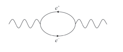
Figure 1.1: First order, $\alpha$, vacuum polarization Feynman diagram contributing to the photon propagator

Qualitatively it can be thought of as a photon splitting into a virtual $e^{+}e^{-}$ pair, so at the quantum level it is characterized by the Compton wavelength $\lambda_{c}$; then, when this quantum cloud of size $\mathcal{O}(\lambda_{c})$ passes through a curved spacetime its motion would be affected differently to that described by general relativity, possibly in a polarization-dependent way [5].

This effect of vacuum polarization is considered through the effective action:

$$S=S_{1}+S_{2}$$ (1.4)

where $S_{1}$ is the Maxwell electromagnetic action in curved space time:

$$S_{1} = -\frac{1}{4}\int d^{4}x\sqrt{-g}F_{\mu\nu}F^{\mu\nu}$$

$$F_{\mu\nu} = \partial_{\mu}A_{\nu}-\partial_{\nu}A_{\mu}$$ (1.5)

and $S_{2}$ is the part of the action that incorporates the effects of virtual electron loops in a background gravitational field. As we are only concerned with the propagation of individual photons it must be quadratic in $A_{\mu}$, and the constraint of gauge invariance then implies that it must depend on $F_{\mu\nu}$ rather than $A_{\mu}$. Also, as the virtual loops give the photon a size of $\lambda_{c}$, $S_{2}$ can be expanded in powers of $\lambda_{c}^{2}=m^{-2}$, thus the lowest term in the expansion would be of order $m^{-2}$, which is the term corresponding to one electron loop. With these constraints there are only four independent gauge invariant terms, which can be chosen to be:

$$S_{2} = \frac{1}{m^{2}}\int d^{4}x\sqrt{-g}(aRF_{\mu\nu}F^{\mu\nu}+bR_{\mu\nu}F^{\mu\sigma}F^{\nu}_{\sigma}$$ (1.6)

$$+ cR_{\mu\nu\sigma\tau}F^{\mu\nu}F^{\sigma\tau}+dD_{\mu}F^{\mu\nu}D_{\sigma}F^{\sigma}_{\nu})$$

The first three terms represent a direct coupling of the electromagnetic field to the curvature, and they vanish in flat-spacetime. The fourth, however, is also applicable in the case of flat-spacetime, and represents off-mass-shell effects in the vacuum polarization. In [1] the values for $a$, $b$, $c$, and $d$ have been determined to $\mathcal{O}(e^{2})$. The constant $d$ is obtained by comparing the coefficient of the renormalized flat-spacetime photon propagator associated with the Feynman diagram in Fig. 1.1 to the result of the same order given by the effective action $S$; and $a$, $b$, and $c$ are obtained by comparing the coefficients of the coupling of a graviton to two photons to the same result obtained from $S_{2}$. In this way the constants are given as:

$$a=-\frac{5}{720}\frac{\alpha}{\pi}\qquad b=\frac{26}{720}\frac{\alpha}{\pi}\qquad c=-\frac{2}{720}\frac{\alpha}{\pi}\qquad d=-\frac{24}{720}\frac{\alpha}{\pi}$$ (1.7)

Then, as the equations of motion for the electromagnetic field are given by:

$$\frac{\delta S}{\delta A_{\mu}(x)}=0$$ (1.8)

using the modified action (1.4) we find:

$$D_{\mu}F^{\mu\nu}+\frac{\delta S_{2}}{\delta A_{\mu}}=0$$ (1.9)

From this we can see that $D_{\mu}F^{\mu\nu}$ is of $\mathcal{O}(e^{2})$, therefore, the term with coefficient $d$ in Eqn. (1.6) will be of $\mathcal{O}(e^{4})$, hence we can omit it from the final equation of motion. In this way we find [7]:

$$D_{\mu}F^{\mu\nu}-\frac{1}{m_{e}^{2}}[2bR_{\mu\lambda}D^{\mu}F^{\lambda\nu}+4cg^{\nu\tau}R_{\mu\tau\lambda\rho}D^{\mu}F^{\lambda\rho}]=0$$ (1.10)

which is the Maxwell equation in curved spacetime, incorporating the coupling of curvature with vacuum polarization effects. Using this modified Maxwell equation and the methods of geometric optics (described in Chapter 3) it is possible to derive the quantum modified light cone and geodesic equations. Then, using these, we are able to determine the quantum modified trajectories in curved spacetime.

1.3 The Equivalence Principle and Causality

The equivalence principle exists in two forms: weak and strong. The weak equivalence principle states that at each point in spacetime there exists a local Minkowski frame, which is a fundamental requirement of general relativity. The strong equivalence principle (SEP), on the other hand, states that the laws of physics are the same in all LIFs at different points in spacetime, and at the origin of each LIF they take the special relativistic form. Then the coupling of curvature to the electromagnetic field in the effective action, Eqn. (1.4), is a violation of the SEP. Due too this violation of the SEP, QED in curved spacetime remains a causal theory - despite the modification to the physical light cone.

This can be seen more clearly by considering Global Lorentz invariance (GLI), which is the special relativistic equivalent of the SEP. In special relativity GLI states that faster than light signals automatically imply the possibility of unacceptable closed-time-loops, Fig. 1.2. That is, if you can send a signal backwards in time in one frame, then it should be possible in any frame. However, if you break this GLI, a signal backwards in time in one frame does not automatically imply you can send a signal backwards in time from any frame. Therefore, in the case of QED in curved spacetime, due to the breakdown of the SEP we retain the fundamental property of causality: faster than light signals can be seen to go backwards in time in a certain frame, but this no longer implies that you can send a signal backwards in time from any frame. Thus, in this case, spacelike motion does not necessarily imply a causality violation.

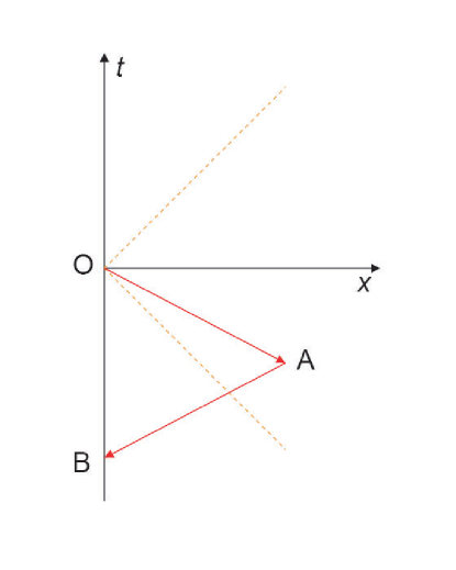
Figure 1.2: An unacceptable closed-time-loop.

1.4 Critical Stable Orbits

One of the simplest curved spacetimes is the (Ricci-flat) Schwarzschild spacetime, which describes the spherically symmetric geometry outside a star. The geometry of such a spacetime structure is given by the line interval:

$$ds^{2}=(1-\frac{2M}{r})dt^{2}-(1-\frac{2M}{r})^{-1}dr^{2}-r^{2}d\theta^{2}-(r^{2}\sin^{2}\theta)d\phi^{2}$$ (1.11)

In this spacetime the equations of motion, derived for $k^{2}=0$, have a special solution for null geodesics. This solution describes a light ray in a circular orbit with a radius $r=3M$ and an associated critical impact parameter. Therefore, a photon projected from $r\rightarrow\infty$ with the critical parameter tends to the stable circular orbit by spiralling around it. But, in the context of vacuum polarization effects, we may derive the null equation of motion using the quantum modified Maxwell equation. In this way the orbit equation should give us stable circular orbits that are dependent on the photon polarization, i.e. splitting the circular orbit depending on polarization. Therefore, a photon coming in from $r\rightarrow\infty$, with a particular polarization and impact parameter, should tend to its associated critical stable orbit by spiralling around it in the classic way.

Chapter 2 Null Dynamics in Schwarzschild Spacetime

In this chapter we will give a brief overview of null dynamics in Schwarzschild spacetime. Starting with the geodesic equations and the line interval for photons we will derive the orbit equation, which will then be used to determine the critical stable orbit for photons and the associated impact parameter. We will then go on to show that decreasing the impact parameter, from the critical value, causes the photon trajectory, given as a function of $\phi$, to spiral into the singularity, but as a function of $t$ it tends to the event horizon. The main aim of this chapter is to familiarise ourselves with the classical solutions of photon trajectories in Schwarzschild spacetime, so we can then compare the equivalent results for the quantum modified case.

2.1 Equations of Motion

When we consider motion in a plane, where $\theta=\frac{\pi}{2}$ and $\dot{\theta}=\ddot{\theta}=0$, the geodesic equations for Schwarzschild spacetime, (A.10)-(A.13), can written as:

$$(1-\frac{2M}{r})\ddot{t}+\frac{2M}{r^{2}}\dot{r}\dot{t}=0$$ (2.1)

$$\frac{M}{r^{2}}\dot{t}^{2}-r\dot{\phi}^{2}+(1-\frac{2M}{r})^{-1}\ddot{r}-\frac{M}{r^{2}}(1-\frac{2M}{r})^{-2}\dot{r}^{2}=0$$ (2.2)

$$2r\dot{r}\dot{\phi}+r^{2}\ddot{\phi}=0$$ (2.3)

And the spacetime line interval becomes:

$$(1-\frac{2M}{r})\dot{t}^{2}-(1-\frac{2M}{r})^{-1}\dot{r}^{2}-r^{2}\dot{\phi}^{2}=K$$ (2.4)

where $K=0$ for photons and $\pm 1$ for space-like or time-like motion. Now, to derive the orbit equation $\frac{du}{d\phi}$ we use Eqns. (2.1), (2.3) and the interval equation (2.4), in the simplified form:

$$0 = \ddot{t}+\frac{2M}{r^{2}}(1-\frac{2M}{r})^{-1}\dot{r}\dot{t}$$ (2.5)

$$0 = \ddot{\phi}+\frac{2\dot{r}}{r}\dot{\phi}$$ (2.6)

$$K(1-\frac{2M}{r}) = -\dot{r}^{2}+(1-\frac{2M}{r})^{2}\dot{t}^{2}-r^{2}(1-\frac{2M}{r})\dot{\phi}^{2}$$ (2.7)

In order to specify photon trajectories we can set $K=0$ at anytime, however, then $\tau$ would be interpreted as an affine parameter and not proper time. To proceed we divide (2.5) by $\frac{dt}{d\tau}$ and (2.6) by $\frac{d\phi}{d\tau}$:

$$0 = \frac{\ddot{t}}{\dot{t}}+\frac{2M}{r^{2}}(1-\frac{2M}{r})^{-1}\dot{r}$$ (2.8)

$$0 = \frac{\ddot{\phi}}{\dot{\phi}}+\frac{2\dot{r}}{r}$$ (2.9)

These can written as:

$$0 = \frac{d}{d\tau}(\ln{\dot{t}}+\ln(1-\frac{2M}{r}))$$ (2.10)

$$0 = \frac{d}{d\tau}(\ln{\dot{\phi}}+\frac{2\dot{r}}{r})$$ (2.11)

Then, solving these we have:

$$\dot{t} = (1-\frac{2M}{r})^{-1}E$$ (2.12)

$$\dot{\phi} = \frac{J}{r^{2}}$$ (2.13)

Where $E$ and $J$ are constants of integration denoting total energy and angular momentum about an axis normal to the plane $\theta=\pi/2$. Now, using Eqns. (2.12) and (2.13) to substitute for $\dot{t}$ and $\dot{\phi}$ in Eqn (2.7) and rearranging, we have:

$$\dot{r}^{2}+r^{2}(1-\frac{2M}{r})\frac{J^{2}}{r^{4}}+K(1-\frac{2M}{r})=(1-\frac{2M}{r})^{2}(1-\frac{2M}{r})^{-1}E^{2}$$ (2.14)

Rearranging and simplifying, this becomes:

$$(\frac{dr}{d\tau})^{2}+(1-\frac{2M}{r})(K+\frac{J^{2}}{r^{2}})=E^{2}$$ (2.15)

$$(\frac{dr}{d\tau})=E[1-(1-\frac{2M}{r})(\frac{K}{E^{2}}+\frac{J^{2}}{E^{2}r^{2}})]^{\frac{1}{2}}$$ (2.16)

We now have the components of the four momentum $P^{\alpha}$ in spherical polar coordinates

$$P^{\alpha} = (\dot{t},\dot{r},\dot{\theta},\dot{\phi})$$ (2.17)

$$= E(F^{-1},[1-F(\frac{K}{E^{2}}+\frac{D^{2}}{r^{2}})]^{\frac{1}{2}},0,\frac{D}{r^{2}})$$

where $D=\frac{J}{E}$ is the impact parameter, $F=(1-\frac{2M}{r})$ and $K=0$ for photons and $K=+1$ for particles.

2.1.1 Orbit Equation

In order to derive orbit equations that are physically understandable we need to represent them as $r(\phi)$, $r(t)$ and $\phi(t)$. In this form we can analyse the orbit paths as a function of rotational angle $\phi$ and the time taken to reach a certain point along the angle. Therefore, by using

$$\frac{dr}{d\tau}=\frac{dr}{d\phi}\cdot\frac{d\phi}{d\tau}=\frac{dr}{d\phi}\frac{J}{r^{2}}$$ (2.18)

we can rewrite (2.15) as

$$E^{2} = (\frac{dr}{d\phi})^{2}\frac{J^{2}}{r^{4}}+(1-\frac{2M}{r})(K+\frac{J^{2}}{r^{2}})$$

$$\Rightarrow\qquad(\frac{dr}{d\phi})^{2} = (E^{2}-K)\frac{r^{4}}{J^{2}}+2MK\frac{r^{3}}{J^{2}}-r^{2}+2Mr$$ (2.19)

Now, transforming $u=r^{-1}$, so at $r=\infty$ we have $u=0$, Eqn. (2.19) becomes:

$$(\frac{du}{d\phi})^{2}r^{4} = (E^{2}-K)\frac{r^{4}}{J^{2}}+2MK\frac{r^{3}}{J^{2}}-r^{2}+2Mr$$

$$(\frac{du}{d\phi})^{2} = \frac{(E^{2}-K)}{J^{2}}+2MK\frac{u}{J^{2}}-u^{2}+2Mu^{3}$$ (2.20)

Doing similar manipulation for $\phi(t)$ we have

$$\frac{d\phi}{dt}=\frac{d\phi}{d\tau}\cdot\frac{d\tau}{dt}$$ (2.21)

and using Eqns. (2.12) and (2.13) in this, and transforming $u=\frac{1}{r}$, we have:

$$\frac{d\phi}{dt}=\frac{D}{r^{2}}(1-\frac{2M}{r})=Du^{2}(1-2Mu)$$ (2.22)

Finally, we can determine $u(t)$ by inserting:

$$\frac{du}{d\phi}=\frac{du}{dt}\cdot\frac{dt}{d\phi}=\frac{du}{dt}[Du^{2}(1-2Mu)]^{-1}$$ (2.23)

into Eqn. (2.20), which gives

$$(\frac{du}{dt})^{2}=[Du^{2}(1-2Mu)]^{2}[\frac{(E^{2}-K)}{J^{2}}+2MK\frac{u}{J^{2}}-u^{2}+2Mu^{3}]$$ (2.24)

Now, the Eqns. (2.20), (2.22) and (2.24) are the general equations that determine photon and particle trajectories in the plane $\theta=\pi/2$. If we take $K=0$ we then have the required photon trajectory equations

$$(\frac{du}{d\phi})^{2} = \frac{1}{D^{2}}-u^{2}+2Mu^{3}=f(u)$$ (2.25)

$$(\frac{du}{dt})^{2} = [Du^{2}(1-2Mu)]^{2}[\frac{1}{D^{2}}-u^{2}+2Mu^{3}]$$ (2.26)

$$= [Du^{2}(1-2Mu)]^{2}f(u)$$

We can also write another equation, specifically for null radial geodesics. By using the fact that $\dot{\phi}=0$, Eqn. (2.13) implies $J=0$, then Eqns (2.12) and (2.15) become

$$(1-\frac{2M}{r})\frac{dt}{d\tau}=E$$ (2.27)

$$\frac{dr}{d\tau}=\pm E$$ (2.28)

Combining these we have:

$$\frac{dr}{dt}=\pm(1-\frac{2M}{r})$$ (2.29)

2.2 Orbits in Schwarzschild Spacetime

We will now discuss the solutions of Eqns. (2.25), (2.26) and (2.29). We will start off with the simple case of the radial geodesic and then go onto the case of the general orbits. For the general case we will solve (2.25) and (2.26) to determine the critical stable orbits and the associated impact parameters. We will then go on to study the trajectories of photons as they fall into the singularity

2.2.1 Null Radial Geodesic

Eqn. (2.29) can be solved by rewriting it as:

$$\frac{dt}{dr} = \pm(1-\frac{2M}{r})^{-1}$$ (2.30)

$$\Rightarrow\qquad t = \pm(r+2M\log(\frac{r}{2M}-1))+constant_{\pm}$$ (2.31)

This solution (specifically the $-$ one) gives the trajectory of a photon coming from infinity and into the black hole. It shows that the photon takes an infinite coordinate time to reach the horizon, which can be seen in Fig. 2.1. However, if we solve Eqn. (2.28), i.e. in terms of the affine parameter, we can show that the photon reaches and crosses the event horizon without ever noticing it,

$$r=\pm E\tau+constant_{\pm}$$ (2.32)

this can be seen in Fig. 2.2

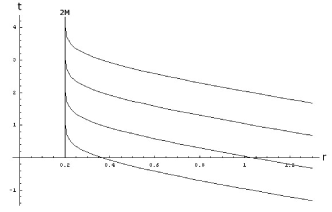
Figure 2.1: Radial Null geodesics take an infinite coordinate time to reach the event horizon at 2M

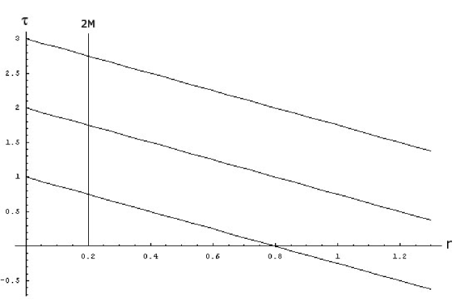
Figure 2.2: Radial Null geodesics reach and cross the event horizon at 2M without noticing it when defined with the affine parameter

2.2.2 General Null Geodesics and Critical Orbits

We will first solve Eqn. (2.25) in order to determine the the critical stable photon orbits. In order to do this we first consider the point of equilibrium and the associated impact parameter. This equilibrium point occurs when

$$\frac{du}{d\phi}=0$$ (2.33)

which means as the photon is orbiting the black hole $u$ does not change; so if the radial distance does not change it implies a circular orbit. Therefore we must solve

$$f(u)=\frac{1}{D^{2}}-u^{2}+2Mu^{3}=0$$ (2.34)

The sum and product of the roots $u_{1}$, $u_{2}$, and $u_{3}$ of this equation are given by

$$u_{1}+u_{2}+u_{3}=\frac{1}{2M}\qquad\textrm{and}\qquad u_{1}u_{2}u_{3}=-\frac{1}{2MD^{2}}$$ (2.35)

This shows that $f(u)=0$ must have a real negative root, and the two remaining roots can be real (distinct or coincident) or be a complex conjugate pair; however, the occurrence of coincident positive real roots implies the existence of a circular orbit. Thus, if a coincident root occurs it should be at the point given by the derivative of $f(u)$

$$f^{\prime}(u)=6Mu^{2}-2u=0$$ (2.36)

Which then has the solution $u_{1}=u_{2}=(3M)^{-1}$. For this solution the impact parameter of equation (2.34) is $D=(3\sqrt{3})M$. From the product condition, equation (2.35), we find that the roots of $f(u)=0$ are

$$u_{1}=u_{2}=\frac{1}{3M}\qquad\textrm{and}\qquad u_{3}=-\frac{1}{6M}\qquad\textrm{and}\qquad D=(3\sqrt{3})M$$ (2.37)

Therefore, when the impact parameter is $D=(3\sqrt{3})M$ then $\frac{du}{d\phi}$ vanishes for $u=(3M)^{-1}$, which implies a circular orbit of radius $3M$ is an allowed null geodesic [2].

Now we can consider a photon at $u=0$ with an impact parameter $D=(3\sqrt{3})M$. This, then, gives a trajectory of a photon spiralling in and tending to the critical orbit at $u=(3M)^{-1}$. The general differential equation for this impact parameter is given by rearranging and substituting for $D$ in Eqn. (2.25)

$$(\frac{du}{d\phi})^{2}=2M(u+\frac{1}{6M})(u-\frac{1}{3M})^{2}$$ (2.38)

From [2] we have the solution to this as

$$u=-\frac{1}{6M}+\frac{1}{2M}\tanh^{2}{\frac{1}{2}(\phi-\phi_{0})}$$ (2.39)

where $\phi_{0}$ is a constant of integration, given by:

$$\tanh^{2}{(-\frac{1}{2}\phi_{0})}=\frac{1}{3},$$ (2.40)

which gives: $u=0$ ($r\rightarrow\infty$) when $\phi=0$, and $u=\frac{1}{3M}$ when $\phi\rightarrow\infty$. Therefore a null geodesic arriving from infinity with an impact parameter $D=(3\sqrt{3})M$ approaches the circle of radius $3M$, asymptotically, by spiralling around it, as can be seen in Fig. 2.3. Also, numerically solving Eqn (2.26) we can show that as time increases $u$ tends to $\frac{1}{3M}$, which can be seen in Fig. 2.4.

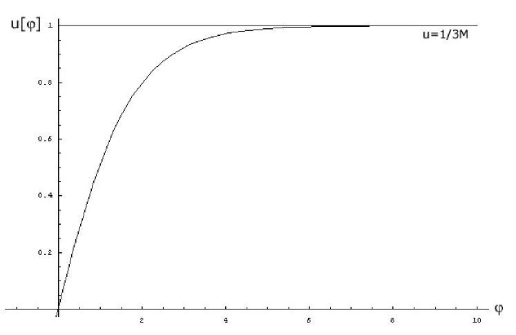
Figure 2.3: Null geodesic, with impact parameter $D=(3\sqrt{3})M$, arriving from infinity and approaching $u=\frac{1}{3M}$ asymptotically (M=1/3)

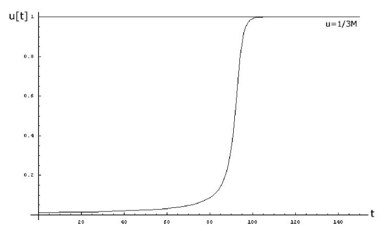
Figure 2.4: For impact parameter $D=(3\sqrt{3})M$ a null trajectory tends to $u=\frac{1}{3M}$ asymptotically with time.

Finally we can show that when an impact parameter other than $D=(3\sqrt{3})M$ is used, for example if we set $D=(3\sqrt{3})M-0.1$, the solution of Eqn. (2.25) shows that the photon falls past the critical orbit, through the event horizon, and into the singularity, Fig. 2.5. Using this new impact parameter in Eqn. (2.26) and, again solving numerically, we see that the photon comes in from infinity and tends to the event horizon, $u=\frac{1}{2M}$, asymptotically in time $t$, Fig. 2.6.

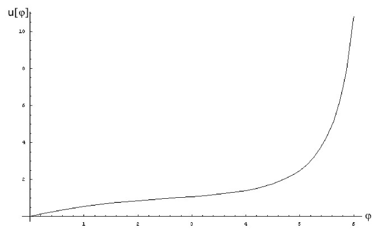
Figure 2.5: Null geodesic, with impact perimeter $D=(3\sqrt{3})M-0.1$, arrives from infinity and spirals into the singularity.

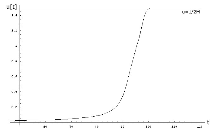
Figure 2.6: Null geodesic, with impact perimeter $D=(3\sqrt{3})M-0.1$, arrives from infinity and tends to $u=\frac{1}{2M}$ asymptotically in time $t$.

Chapter 3 Quantum Gravitational Optics

3.1 Photon Propagation in Curved Spacetime

Maxwell’s equations, in curved spacetime,

$$0=D_{\mu}F^{\mu\nu}$$ (3.1)

$$0 = D_{\mu}F_{\nu\lambda}+D_{\nu}F_{\lambda\mu}+D_{\lambda}F_{\mu\nu}$$ (3.2)

$$\Rightarrow F_{\mu\nu}=\partial_{\mu}A_{\nu}-\partial_{\nu}A_{\mu},$$ (3.3)

cannot be solved explicitly, and even in cases of extreme symmetry explicit solutions are difficult; this is due to the fact that as curved space acts as a dispersive material (i.e. bending light rays) plane wave solutions do not exist.

3.1.1 Geometric Optics in Curved Spacetime

In dispersive materials, where light rays are bent, we can consider the solution of Maxwell’s equations to be a simple perturbation of the plane wave solution. For example in curved space, relative to an observer, the electromagnetic waves can appear to be plane and monochromatic on a scale that is much larger compared to the typical wavelength, but very small compared with the typical radius of curvature of space time. Such "locally plane" waves can be represented, in geometric optics, by approximate solutions of Maxwell’s equations of the form[6]:

$$\mathcal{F}^{\mu\nu}=Re(F_{1}^{\mu\nu}+i\varepsilon F_{2}^{\mu\nu}+\ldots)e^{i\frac{\theta}{\varepsilon}}$$ (3.4)

and the electromagnetic field vector, defined by Eqn. (3.3), takes the form:

$$\mathcal{A}^{\mu}=Re(A_{1}^{\mu}+i\varepsilon A_{2}^{\mu}+\ldots)e^{i\frac{\theta}{\varepsilon}}$$ (3.5)

where the electromagnetic field is written as a slowly-varying amplitude and a rapidly-varying phase. The parameter $\varepsilon$ is introduced in order to keep track of the relative order of magnitude of terms, so in curved space Maxwell’s equations can be solved order-by-order in $\varepsilon$. In this formulation the wave vector is then defined as the gradient of the phase of the field, $k_{\mu}=D_{\mu}\frac{i}{\varepsilon}\theta=\partial_{\mu}\frac{i}{\varepsilon}\theta$, which in terms of the quantum interpretation is identified as the photon momentum. We can also write $A^{\mu}=Aa^{\mu}$, where $A$ represents the amplitude and $a_{\mu}$ (normalized as $a_{\mu}a^{\mu}=-1$) specifies the wave polarization. These vectors then satisfy the condition $k_{\mu}a^{\mu}=0$.

Geometric Optics and Null Dynamics

In this notation Eqn. (3.1) can be written, to leading order $\mathcal{O}(\frac{1}{\varepsilon})$, as:

$$\partial_{\mu}(F_{1}^{\mu\nu}e^{i\frac{\theta}{\varepsilon}}) = F_{1}^{\mu\nu}e^{i\frac{\theta}{\varepsilon}}(\frac{i}{\varepsilon}\partial_{\mu}\theta)$$

$$\Rightarrow\qquad k_{\mu}F_{1}^{\mu\nu} = 0$$ (3.6)

and Eqn. (3.3) becomes:

$$F_{1\mu\nu}e^{i\frac{\theta}{\varepsilon}} = (\partial_{\mu}A_{1\nu}-\partial_{\nu}A_{1\mu})e^{i\frac{\theta}{\varepsilon}}$$

$$= \frac{i}{\varepsilon}(\partial_{\mu}\theta A_{1\nu}-\partial_{\nu}\theta A_{1\mu})e^{i\frac{\theta}{\varepsilon}}$$

$$\Rightarrow\qquad F_{1\mu\nu} = k_{\mu}A_{1\nu}-k_{\nu}A_{1\mu}$$ (3.7)

Now, by combining these, we have:

$$k_{\mu}F_{1}^{\mu\nu} = k_{\mu}(k^{\mu}A_{1}^{\nu}-k^{\nu}A_{1}^{\mu})=0$$

$$= (k_{\mu}k^{\mu})A_{1}^{\nu}-k^{\nu}(k_{\mu}A_{1}^{\mu})$$

$$\Rightarrow\qquad k^{2}a^{\nu} = 0$$ (3.8)

and from this we can deduce that $k^{2}=0$, i.e. $k^{\mu}$ is a null vector. Also, it follows from the definition of $k^{\mu}$ as a gradient that $D_{\mu}k_{\nu}=D_{\nu}k_{\mu}$, so

$$k^{\mu}D_{\mu}k^{\nu}=k^{\mu}D^{\nu}k_{\mu}=\frac{1}{2}D^{\nu}k^{2}=0$$ (3.9)

Using this, and the fact that light rays are defined as the curves given by $x_{\mu}(s)$ where $\frac{dx_{\mu}}{ds}=k_{\mu}$, we can derive the geodesic equation as follows[7]:

$$0 = k^{\mu}D_{\mu}k^{\nu}$$ (3.10)

$$= \frac{d^{2}x^{\nu}}{ds^{2}}+\Gamma^{\nu}_{\mu\lambda}\frac{dx^{\mu}}{ds}\frac{dx^{\lambda}}{ds}$$

3.2 Quantum Modified Null Dynamics

As was seen in Sec. 1.2, using the effective action, Eqn. (1.4), the equation of motion becomes:

$$0=D_{\mu}F^{\mu\nu}-\frac{1}{m^{2}}[2bR_{\mu\lambda}D^{\mu}F^{\lambda\nu}+4cg^{\nu\tau}R_{\mu\tau\lambda\rho}D^{\mu}F^{\lambda\rho}]$$ (3.11)

and the Bianchi identity, Eqn. (3.2), remains unchanged. Now, as before we can determine the quantum modified light cone and geodesic equations.

Quantum Modified Light Cone

Substituting Eqn. (3.4) in (3.11) we find, again to $\mathcal{O}(\frac{1}{\varepsilon})$:

$$0=\frac{i}{\varepsilon}(D_{\mu}\theta)e^{i\frac{\theta}{\varepsilon}}F_{1}^{\mu\nu} - \frac{1}{m^{2}}[2bR_{\mu\lambda}\frac{i}{\varepsilon}(D^{\mu}\theta)e^{i\frac{\theta}{\varepsilon}}F_{1}^{\lambda\nu}$$

$$+ 4cg^{\nu\tau}R_{\mu\tau\lambda\rho}\frac{i}{\varepsilon}(D^{\mu}\theta)e^{i\frac{\theta}{\varepsilon}}F_{1}^{\lambda\rho}]$$

$$\Rightarrow\qquad 0=k_{\mu}F_{1}^{\mu\nu}-\frac{1}{m_{e}^{2}}[2bR_{\mu\lambda}k^{\mu}F_{1}^{\lambda\nu}+4cg^{\nu\tau}R_{\mu\tau\lambda\rho}k^{\mu}F_{1}^{\lambda\rho}]$$ (3.12)

and using Eqn. (3.7) we have:

$$0=k_{\mu}(k^{\mu}A_{1}^{\nu}-k^{\nu}A_{1}^{\mu}) - \frac{1}{m_{e}^{2}}[2bR_{\mu\lambda}k^{\mu}(k^{\lambda}A_{1}^{\nu}-k^{\nu}A_{1}^{\lambda})$$

$$+ 4cg^{\nu\tau}R_{\mu\tau\lambda\rho}k^{\mu}(k^{\lambda}A_{1}^{\rho}-k^{\rho}A_{1}^{\lambda})]$$

using $k_{\mu}A^{\mu}=0$ this becomes:

$$0=k_{\mu}k^{\mu}A_{1}^{\nu} - \frac{1}{m_{e}^{2}}[2bR_{\mu\lambda}k^{\mu}(k^{\lambda}A_{1}^{\nu}-k^{\nu}A_{1}^{\lambda})$$ (3.13)

$$+ 4cg^{\nu\tau}R_{\mu\tau\lambda\rho}k^{\mu}(2k^{\lambda}A_{1}^{\rho})]$$

where $A_{1}^{\nu}=A_{1}a^{\nu}$, and the last line is simplified by relabeling of indices. Now, Contracting with $Aa_{\nu}$ and eliminating $A$ we have:

$$0=-k_{\mu}k^{\mu}+\frac{2b}{m_{e}^{2}}R_{\mu\lambda}k^{\mu}k^{\lambda}-\frac{8c}{m_{e}^{2}}R_{\mu\tau\lambda\rho}k^{\mu}k^{\lambda}a_{1}^{\tau}a_{1}^{\rho}$$

This then gives the quantum modified light cone:

$$k^{2}-\frac{2b}{m^{2}}R_{\mu\lambda}k^{\mu}k^{\lambda}-\frac{8c_{\alpha}}{m_{e}^{2}}R_{\mu\tau\lambda\rho}k^{\mu}k^{\lambda}a^{\tau}a^{\rho}=k^{2}-\delta k(a)=0$$ (3.14)

where we have replaced the constant $c=-\frac{\alpha}{360\pi}$ with $c_{\alpha}=\frac{\alpha}{360\pi}$ for convenience of interpretation, i.e. the sign of the light cone is immediately obvious from $R_{\mu\tau\lambda\rho}k^{\mu}k^{\lambda}a^{\tau}a^{\rho}$. As we will be working in the Schwarzschild spacetime the quantum modified light cone for the Ricci flat case ($R_{\mu\lambda}=0$) is given by:

$$k^{2}=\frac{8c_{\alpha}}{m_{e}^{2}}R_{\mu\tau\lambda\rho}k^{\mu}k^{\lambda}a^{\tau}a^{\rho}=\delta k(a)$$ (3.15)

Here the sign of the light cone depends on polarization and the photon trajectory; if the correction is positive we have space-like motion, and if it’s negative we have time-like motion.

Quantum Modified Geodesic Equation

The photon trajectories corresponding to the quantum modified equation of motion, (3.11), can be represented by a generalised version of Eqn. (3.9):

$$0 = \frac{1}{2}D_{\nu}[k^{2}-\frac{2b}{m^{2}}R_{\mu\lambda}k^{\mu}k^{\lambda}-\frac{8c_{\alpha}}{m_{e}^{2}}R_{\mu\tau\lambda\rho}k^{\mu}k^{\lambda}a^{\tau}a^{\rho}]$$

$$0 = \frac{1}{2}D_{\nu}k^{2}-\frac{1}{m^{2}}D_{\nu}[bR_{\mu\lambda}k^{\mu}k^{\lambda}+4c_{\alpha}R_{\mu\tau\lambda\rho}k^{\mu}k^{\lambda}a^{\tau}a^{\rho}]$$

$$\Rightarrow\qquad 0 = \frac{d^{2}x^{\nu}}{ds^{2}}+\Gamma_{\mu\lambda}^{\nu}\frac{dx^{\mu}}{ds}\frac{dx^{\lambda}}{ds}$$ (3.16)

$$- \frac{1}{m^{2}}\partial_{\nu}[(bR_{\beta\gamma}+4c_{\alpha}R_{\beta\sigma\gamma\tau}a^{\sigma}a^{\tau})\frac{dx^{\beta}}{ds}\frac{dx^{\gamma}}{ds}]$$

where we have used $k^{\mu}=\frac{dx^{\mu}}{ds}$, and covariant derivative in the second term is replaced by a partial derivative as it’s acting on a scalar. In Ricci spacetime this equation becomes:

$$0=\frac{d^{2}x^{\nu}}{ds^{2}}+\Gamma_{\mu\lambda}^{\nu}\frac{dx^{\mu}}{ds}\frac{dx^{\lambda}}{ds}-\frac{4c_{\alpha}}{m^{2}}\partial_{\nu}[R_{\beta\sigma\gamma\tau}a^{\sigma}a^{\tau}\frac{dx^{\beta}}{ds}\frac{dx^{\gamma}}{ds}]$$ (3.17)

3.3 Horizon Theorem and Polarization Rule

There are two general features associated with quantum modified photon propagation[7]. First, it is a general result that the velocity of radially directed photons remains equal to $c$ at the event horizon. Second, for Ricci flat spacetimes (such as Schwarzschild[1] and Kerr[8] spacetimes), the velocity shifts for the two transverse polarizations are always equal and opposite. However, this is no longer true for non-Ricci flat cases (such as Robertson-Walker spacetime[1]). In these cases, the polarization averaged velocity shift is proportional to the matter energy-momentum tensor. These features can be easily shown by using the Newman-Penrose formalism: this characterises spacetimes using a set of complex scalars, which are found by contracting the Weyl tensor with elements of a null tetrad[2].

Newman-Penrose Formalism

We choose the basis vectors of the null tetrad as[7]: $l^{\mu}=k^{\mu}$, the photon momentum. Then, we denote the two spacelike, normalized, transverse polarization vectors by $a^{\mu}$ and $b^{\mu}$ and construct the null vectors $m^{\mu}=\frac{1}{\sqrt{2}}(a^{\mu}+ib^{\mu})$ and $\bar{m}^{\mu}=\frac{1}{\sqrt{2}}(a^{\mu}-ib^{\mu})$. We complete the tetrad with a further null vector $n^{\mu}$, which is orthogonal to $m^{\mu}$ and $\bar{m}^{\mu}$. We then have the conditions:

$$l\cdot m=l\cdot\bar{m}=n\cdot m=n\cdot\bar{m}=0$$ (3.18)

from orthogonality, and:

$$l\cdot l=n\cdot n=m\cdot m=\bar{m}\cdot\bar{m}=0$$ (3.19)

since the basis vectors are null. Finally, we impose:

$$l\cdot n=-m\cdot\bar{m}=1$$ (3.20)

The Weyl tensor, given in terms of the Riemann and Ricci tensors, is:

$$C_{\mu\nu\gamma\delta}=R_{\mu\nu\gamma\delta} - \frac{1}{2}(\eta_{\mu\gamma}R_{\nu\delta}-\eta_{\nu\gamma}R_{\mu\delta}-\eta_{\mu\delta}R_{\nu\gamma}+\eta_{\nu\delta}R_{\mu\gamma})$$ (3.21)

$$+ \frac{1}{6}(\eta_{\mu\gamma}\eta_{\nu\delta}-\eta_{\mu\delta}\eta_{\nu\gamma})R$$

where $R_{\mu\gamma}=\eta^{\nu\delta}R_{\mu\nu\gamma\delta}$ and $R=\eta^{\mu\nu}R_{\mu\nu}$; and the Weyl tensor satisfies the trace-free condiation:

$$\eta^{\mu\delta}C_{\mu\nu\gamma\delta}=0$$ (3.22)

and the cyclicity property:

$$C_{1234}+C_{1342}+C_{1423}=0$$ (3.23)

Now, using the null tetrad, we can denote the ten independent components of the Weyl tensor by the five complex Newman-Penrose scalars:

$$\Psi_{0} = -C_{\mu\nu\gamma\delta}l^{\mu}m^{\nu}l^{\gamma}m^{\delta}$$

$$\Psi_{1} = -C_{\mu\nu\gamma\delta}l^{\mu}n^{\nu}l^{\gamma}m^{\delta}$$

$$\Psi_{2} = -C_{\mu\nu\gamma\delta}l^{\mu}m^{\nu}\bar{m}^{\gamma}n^{\delta}$$

$$\Psi_{3} = -C_{\mu\nu\gamma\delta}l^{\mu}n^{\nu}\bar{m}^{\gamma}n^{\delta}$$

$$\Psi_{4} = -C_{\mu\nu\gamma\delta}n^{\mu}\bar{m}^{\nu}n^{\gamma}\bar{m}^{\delta}$$ (3.24)

3.3.1 Polarization Sum Rule

Ricci Flat Spacetime

In Ricci flat spacetime, summing the quantum correction over the two polarizations leads to the following polarization sum rule:

$$\sum_{a}\delta k(a)=0$$ (3.25)

This can be proven by suming the quantum correction in Eqn. (3.15) over the two polarizations,

$$\sum_{a}\delta k(a)=\frac{8c_{\alpha}}{m_{e}^{2}}\sum_{a}R_{\mu\nu\gamma\delta}k^{\mu}k^{\gamma}a^{\nu}a^{\delta}$$ (3.26)

In the Newman-Penrose basis, using $k=l$, $a=\frac{\sqrt{2}}{2}(m+\bar{m})$, $b=-\frac{i\sqrt{2}}{2}(m-\bar{m})$, and the fact that $C_{\mu\nu\gamma\delta}=R_{\mu\nu\gamma\delta}$ for the Ricci flat case, we have:

$$\sum_{a}R_{\mu\nu\gamma\delta}k^{\mu}k^{\gamma}a^{\nu}a^{\delta} = \frac{1}{2}C_{\mu\nu\gamma\delta}l^{\mu}l^{\gamma}(m^{\nu}+\bar{m}^{\nu})(m^{\delta}+\bar{m}^{\delta})$$ (3.27)

$$- \frac{1}{2}C_{\mu\nu\gamma\delta}l^{\mu}l^{\gamma}(m^{\nu}-\bar{m}^{\nu})(m^{\delta}-\bar{m}^{\delta})$$

$$= C_{\mu\nu\gamma\delta}l^{\mu}l^{\gamma}(m^{\nu}\bar{m}^{\delta}+\bar{m}^{\nu}m^{\delta})$$

This particular contraction is equal to zero as it’s not part of the complex scalars in Eqns. (3.24); hence the sum of the two quantum corrections is zero. This implies the trajectory (and velocity) shifts are equal and opposite.

Non-Ricci Flat Spacetime

For the non-Ricci flat spacetimes the polarization sum rule is given as:

$$\sum_{a}\delta k(a)=-\frac{8\pi}{m_{e}^{2}}(2b-8c_{\alpha})T_{\mu\nu}k^{\mu}k^{\nu}$$ (3.28)

where $T_{\mu\nu}$ is the energy-momentum tensor. This can be shown by proceeding as before, but now we include the Ricci tensor and scalar, as in Eqn. (3.21):

$$\sum_{a}R_{\mu\nu\gamma\delta}k^{\mu}k^{\gamma}a^{\nu}a^{\delta}=C_{\mu\nu\gamma\delta}l^{\mu}l^{\gamma}(m^{\nu}\bar{m}^{\delta}+\bar{m}^{\nu}m^{\delta})-R_{\mu\gamma}l^{\mu}l^{\gamma}$$ (3.29)

As before the first term on the RHS is zero, and the second term is only dependent on the photon momentum. Then, combining this with the Ricci term in Eqn. (3.14) we have:

$$\sum_{a}\delta k(a)=\frac{1}{m_{e}^{2}}(2b-8c_{\alpha})R_{\mu\nu}k^{\mu}k^{\nu}$$ (3.30)

Finally replacing the Ricci tensor with the energy-momentum tensor, by using the Einstein equation

$$R_{\mu\nu}=-8\pi T_{\mu\nu}+\frac{1}{2}Rg_{\mu\nu}$$ (3.31)

we obtain Eqn. (3.28).

3.3.2 Horizon Theorem

At the event horizon, photons with momentum directed normal to the horizon have velocity equal to $c$, i.e. the light cone remains $k^{2}=0$, independent of polarization[7].

This can be easily proven for the Ricci flat spacetime, using the orthonormal vectors $k^{a}=(E_{k},E_{k},0,0)$, $a^{b}=(0,0,1,0)$ and $a^{b}=(0,0,0,1)$. Therefore, using these vectors in Eqn. (3.15), we have:

$$k^{2}=\frac{8c_{\alpha}}{m_{e}^{2}}R_{abcd}k^{a}k^{c}a^{b}a^{d}=0$$ (3.32)

So, in Ricci flat spacetime all radially projected photon trajectories remain unchanged.

It is also possible to prove the horizon theorem for the general case (for Ricci and non-Ricci flat spacetimes) that the light cone at the event horizon is unchanged. This can be seen in the null tetrad, so that the physical, space-like, polarization vectors $a^{\mu}$ and $b^{\mu}$ lie parallel to the event horizon 2-surface, while $k^{\mu}$ is the null vector normal to the surface. Then, from Eqn. (3.14) we have for the two polarizations:

$$k^{2} = \frac{2b}{m_{e}^{2}}R_{\mu\gamma}k^{\mu}k^{\gamma}+\frac{8c_{\alpha}}{m_{e}^{2}}R_{\mu\nu\gamma\delta}k^{\mu}k^{\gamma}a^{\nu}a^{\delta}$$ (3.33)

$$= \frac{2b}{m_{e}^{2}}R_{\mu\gamma}l^{\mu}l^{\gamma}+\frac{8c_{\alpha}}{m_{e}^{2}}[-\frac{1}{2}R_{\mu\gamma}l^{\mu}l^{\gamma}\pm C_{\mu\nu\gamma\delta}l^{\mu}l^{\gamma}\frac{1}{2}(m^{\nu}\pm\bar{m}^{\nu})(m^{\delta}\pm\bar{m}^{\delta})]$$

$$= \frac{1}{m_{e}^{2}}(2b-4c_{\alpha})R_{\mu\gamma}l^{\mu}l^{\gamma}\pm\frac{4c_{\alpha}}{m_{e}^{2}}C_{\mu\nu\gamma\delta}l^{\mu}l^{\gamma}\frac{1}{2}(m^{\nu}\pm\bar{m}^{\nu})(m^{\delta}\pm\bar{m}^{\delta})$$

Using Eqn. (3.31) and the fact that $C_{\mu\nu\gamma\delta}l^{\mu}l^{\gamma}(m^{\nu}\bar{m}^{\delta}+\bar{m}^{\nu}m^{\delta})=0$, we can write this as:

$$k^{2} = -\frac{8\pi}{m_{e}^{2}}(2b-4c_{\alpha})T_{\mu\gamma}l^{\mu}l^{\gamma}\pm\frac{4c_{\alpha}}{m_{e}^{2}}C_{\mu\nu\gamma\delta}l^{\mu}l^{\gamma}(m^{\nu}m^{\delta}+\bar{m}^{\nu}\bar{m}^{\delta})$$ (3.34)

and in terms of the Newman-Penrose scalars this can be written as:

$$k^{2} = -\frac{8\pi}{m_{e}^{2}}(2b-4c_{\alpha})T_{\mu\gamma}l^{\mu}l^{\gamma}\pm\frac{8c_{\alpha}}{m_{e}^{2}}\Psi_{0},$$ (3.35)

where the simplification in the last term on the RHS is possible as $\Psi_{0}$ is real for Schwarzschild spacetime. In general Eqn. (3.35) is non zero, however, at the event horizon the terms: $T_{\mu\gamma}l^{\mu}l^{\gamma}$ and $\Psi_{0}$ are zero for stationary spacetimes[7, 9].

Physically the Ricci term represents the flow of matter across the horizon and the Weyl term represents the flow of gravitational radiation[7], and both are zero in classic general relativity; and as, even with the quantum modification, the light cone remains unchanged at the event horizon, means the event horizon is fixed and light cannot escape from inside the black hole.

Chapter 4 Quantum Modified Trajectories

In this chapter we will analyse how the classical null trajectories, described in Chapter 2, are modified in Schwarzschild spacetime, due to quantum modifications of the equations of motion of general relativity. Using Eqn. (3.14) we will calculate the quantum corrected version of Eqn. (2.25), which will then describe the quantum modified motion of a null trajectory in a Schwarzschild spacetime. Using this, and following the methods of Chapter 2, we will begin by studying simple critical circular orbits at the stationary point, $u=1/3M$. As stated in the polarization rule, the critical orbit should be shifted up and down by equal amounts, depending on the polarization of each photon. Also, we will show that these modifications are only valid if the "classic" impact parameter corresponding to the stationary orbit is adjusted, depending on the photon’s polarization, in order to compensate for the orbit shift. This information, of the modified orbits and the corresponding impact parameter for each polarization, will then be used to determine the general trajectory of a (vertically or horizontally polarized) photon coming in from infinity and tending to one of the two shifted critical orbits. We will then go on to show that these quantum modifications have no effect on the event horizon, that is, when the impact parameter is accordingly adjusted and a photon falls into the singularity the event horizon remains fixed at $u=1/2M$.

4.1 Quantum Modified Circular Orbits

In Schwarzschild spacetime, using $k^{\nu}=dx^{\nu}/d\tau$, Eqn. (3.15) can be written as:

$$0 = \dot{r}^{2}-(1-\frac{2M}{r})^{2}\dot{t}^{2}+r^{2}(1-\frac{2M}{r})\dot{\theta}^{2}$$ (4.1)

$$+ (1-\frac{2M}{r})r^{2}\dot{\phi}^{2}+\frac{8c_{\alpha}}{m_{e}^{2}}(1-\frac{2M}{r})R_{\mu\nu\gamma\delta}k^{\mu}k^{\gamma}a^{\nu}a^{\delta}$$

and Eqn. (3.17) as:

$$0 = \ddot{t}+\frac{2M}{r^{2}}(1-\frac{2M}{r})^{-1}\dot{r}\dot{t}$$ (4.2)

$$- \frac{4c_{\alpha}}{m_{e}^{2}}\partial_{t}(R_{\mu\nu\gamma\delta}a^{\nu}a^{\delta}\frac{dx^{\mu}}{d\tau}\frac{dx^{\gamma}}{d\tau})$$

$$0 = \ddot{r}-\frac{M}{r^{2}}(1-\frac{2M}{r})^{-1}\dot{r}^{2}-r(1-\frac{2M}{r})\dot{\phi}^{2}$$ (4.3)

$$+ \frac{M}{r^{2}}(1-\frac{2M}{r})\dot{t}^{2}-\frac{4c_{\alpha}}{m_{e}^{2}}\partial_{r}(R_{\mu\nu\gamma\delta}a^{\nu}a^{\delta}\frac{dx^{\mu}}{d\tau}\frac{dx^{\gamma}}{d\tau})$$

$$0 = \ddot{\phi}+\frac{2\dot{r}\dot{\phi}}{r}-\frac{4c_{\alpha}}{m_{e}^{2}}\partial_{\phi}(R_{\mu\nu\gamma\delta}a^{\nu}a^{\delta}\frac{dx^{\mu}}{d\tau}\frac{dx^{\gamma}}{d\tau})$$ (4.4)

$$0 = -\frac{4c_{\alpha}}{m_{e}^{2}}\partial_{\theta}(R_{\mu\nu\gamma\delta}a^{\nu}a^{\delta}\frac{dx^{\mu}}{d\tau}\frac{dx^{\gamma}}{d\tau})$$ (4.5)

where $c_{\alpha}=\frac{\alpha}{360\pi}$. Now, in order to consider quantum modified circular orbits we require three things: (i) the Riemann tensor components, (ii) the photon wave vectors, $k^{\mu}=\frac{dx^{\mu}}{d\tau}$, for circular orbits, and finally (iii) the photon polarization vectors, $a^{\mu}$. Due to the circular nature of the orbit the simplest basis to work in is the orthonormal basis. In this frame the required polarization and wave vectors, for circular orbits, are simply given as:

$$a^{\mu}=(0,1,0,0)\qquad\textrm{Planar Polarized}$$ (4.6)

$$a^{\mu}=(0,0,1,0)\qquad\textrm{Vertically Polarized}$$ (4.7)

$$k^{\mu}=\frac{dx^{\mu}}{d\tau}=(E_{k},0,0,E_{k})\qquad\textrm{$4$-momentum along $\phi$}$$ (4.8)

Now using these photon vectors, the quantum modifications in Eqns. (4.1)-(4.5), can be expanded to give:

• For the planar polarized case we have:

  $$R_{abcd}k^{a}k^{c}a^{b}a^{d} = R_{arcr}k^{a}k^{c}=E_{k}^{2}(R_{arcr}\hat{k}^{a}\hat{k}^{c})$$ (4.9)

  $$= E_{k}^{2}(R_{trtr}+R_{\phi r\phi r}+2R_{tr\phi r})$$

• For the vertically polarized case we have:

  $$R_{abcd}k^{a}k^{c}a^{b}a^{d} = R_{a\theta c\theta}k^{a}k^{c}=E_{k}^{2}(R_{a\theta c\theta}\hat{k}^{a}\hat{k}^{c})$$ (4.10)

  $$= E_{k}^{2}(R_{t\theta t\theta}+R_{\phi\theta\phi\theta})$$

Using the six independent components of the Riemann tensor in the orthonormal basis, we find:

$$R_{trrt}=-R_{trtr}=-\frac{2M}{r^{3}}\Rightarrow R_{trtr}=\frac{2M}{r^{3}}$$ (4.11)

$$R_{\phi rr\phi}=-R_{\phi r\phi r}=-\frac{M}{r^{3}}\Rightarrow R_{\phi r\phi r}=\frac{M}{r^{3}}$$ (4.12)

$$R_{\theta t\theta t}=R_{t\theta t\theta}=-\frac{M}{r^{3}}\Rightarrow R_{t\theta t\theta}=-\frac{M}{r^{3}}$$ (4.13)

$$R_{\phi\theta\theta\phi}=-R_{\phi\theta\phi\theta}=\frac{2M}{r^{3}}\Rightarrow R_{\phi\theta\phi\theta}=-\frac{2M}{r^{3}}$$ (4.14)

$$R_{tr\phi r}=0$$ (4.15)

Then Eqns. (4.9) and (4.10) become:

• For the planar polarized case:

  $$R_{abcd}k^{a}k^{c}a^{b}a^{d}=E_{k}^{2}(R_{trtr}+R_{\phi r\phi r}+2R_{tr\phi r})=\frac{3E_{k}^{2}M}{r^{3}}$$ (4.16)

  with the relevant derivatives:

  $$\partial_{t}\frac{3E_{k}^{2}M}{r^{3}} = 0\qquad\partial_{r}\frac{3E_{k}^{2}M}{r^{3}}=-\frac{9E_{k}^{2}M}{r^{4}}$$

  $$\partial_{\theta}\frac{3E_{k}^{2}M}{r^{3}} = 0\qquad\partial_{\phi}\frac{3E_{k}^{2}M}{r^{3}}=0$$ (4.17)

• For the vertically polarized case:

  $$R_{abcd}k^{a}k^{c}a^{b}a^{d}=E_{k}^{2}(R_{t\theta t\theta}+R_{\phi\theta\phi\theta})=-\frac{3E_{k}^{2}M}{r^{3}}$$ (4.18)

  and the relevant derivatives:

  $$-\partial_{t}\frac{3E_{k}^{2}M}{r^{3}} = 0\qquad-\partial_{r}\frac{3E_{k}^{2}M}{r^{3}}=\frac{9E_{k}^{2}M}{r^{4}}$$

  $$-\partial_{\theta}\frac{3E_{k}^{2}M}{r^{3}} = 0\qquad-\partial_{\phi}\frac{3E_{k}^{2}M}{r^{3}}=0$$ (4.19)

From Eqns. (3.15), (4.16) and (4.18) we can see that:

$$k^{2} \sim \frac{3E_{k}^{2}M}{r^{3}}\qquad\textrm{For Planar Polarization}$$ (4.20)

$$k^{2} \sim -\frac{3E_{k}^{2}M}{r^{3}}\qquad\textrm{For Vertical Polarization}$$ (4.21)

This implies that, as the light cone for planar polarization is positive, it represents a photon trajectory with a speed $<c$, and as the light cone for vertical polarization is negative, it represents a photon trajectory with a speed $>c$.

Planar Polarization

Considering the planar polarized case first, we can use Eqns. (4.16) and (4.17) to rewrite Eqns. (4.1)-(4.4) as:

$$0 = \dot{r}^{2}-(1-\frac{2M}{r})^{2}\dot{t}^{2}+r^{2}(1-\frac{2M}{r})\dot{\theta}^{2}$$ (4.22)

$$+ (1-\frac{2M}{r})r^{2}\dot{\phi}^{2}+\frac{8c_{\alpha}}{m_{e}^{2}}(1-\frac{2M}{r})\frac{3E_{k}^{2}M}{r^{3}}$$

$$0 = \ddot{t}+\frac{2M}{r^{2}}(1-\frac{2M}{r})^{-1}\dot{r}\dot{t}$$ (4.23)

$$0 = \ddot{r}-\frac{M}{r^{2}}(1-\frac{2M}{r})^{-1}\dot{r}^{2}-r(1-\frac{2M}{r})\dot{\phi}^{2}$$ (4.24)

$$+ \frac{M}{r^{2}}(1-\frac{2M}{r})\dot{t}^{2}+\frac{4c_{\alpha}}{m_{e}^{2}}\frac{9E_{k}^{2}M}{r^{4}}$$

$$0 = \ddot{\phi}+\frac{2\dot{r}\dot{\phi}}{r}$$ (4.25)

where Eqn. (4.5) becomes zero. Now, using the solutions of (4.23) and (4.25), as given by (2.12) and (2.13), we can rewrite Eqn. (4.22) as a simple quantum modified trajectory equation for circular orbits with radius $r$ and in a plane $\theta=\frac{\pi}{2}$:

$$0 = \dot{r}^{2}-E^{2}+(1-\frac{2M}{r})\frac{J^{2}}{r^{2}}+\frac{8c_{\alpha}}{m_{e}^{2}}(1-\frac{2M}{r})\frac{3E_{k}^{2}M}{r^{3}}$$

$$\Rightarrow\qquad E^{2} = (\frac{dr}{d\tau})^{2}+(1-\frac{2M}{r})(\frac{24cE_{k}^{2}M}{m_{e}^{2}r^{3}}+\frac{J^{2}}{r^{2}})$$ (4.26)

To make this equation more meaningful and easier to solve we make the following transformations:

$$\tau\rightarrow\phi\qquad\frac{dr}{d\phi}\cdot\frac{d\phi}{d\tau}=\frac{dr}{d\phi}\cdot\frac{J}{r^{2}}$$ (4.27)

$$r\rightarrow u=\frac{1}{r}\qquad\frac{du}{d\phi}\cdot\frac{dr}{du}=\frac{du}{d\phi}\cdot(-\frac{1}{u^{2}})$$ (4.28)

Therefore, Eqn. (4.26) becomes:

$$E^{2} = (\frac{dr}{d\phi})^{2}\cdot(\frac{J}{r^{2}})^{2}+(1-\frac{2M}{r})(\frac{24c_{\alpha}E_{k}^{2}M}{m_{e}^{2}r^{3}}+\frac{J^{2}}{r^{2}})$$ (4.29)

$$= (\frac{du}{d\phi})^{2}\cdot(-\frac{1}{u^{2}})^{2}\cdot(Ju^{2})^{2}+(1-2Mu)(\frac{24c_{\alpha}E_{k}^{2}Mu^{3}}{m_{e}^{2}}+J^{2}u^{2})$$

$$= (\frac{du}{d\phi})^{2}\cdot J^{2}+(1-2Mu)(\frac{24c_{\alpha}E_{k}^{2}Mu^{3}}{m_{e}^{2}}+J^{2}u^{2})$$

Which can be written as:

$$(\frac{du}{d\phi})^{2} = 2M^{2}Au^{4}+(2M-MA)u^{3}-u^{2}+\frac{E^{2}}{J^{2}}$$ (4.30)

where we have defined the dimensionless constant:

$$A=\frac{24c_{\alpha}E_{k}^{2}}{J^{2}m_{e}^{2}}=\frac{72c_{\alpha}}{m_{e}^{2}D^{2}},$$ (4.31)

In the last form we have used (without proof) the relation $E_{k}=\sqrt{3}E$, which will be proven in Sec. 4.2.1, Eqn. (4.68).

Vertical Polarization

Similarly, for the vertically polarized case, using Eqns. (4.18) and (4.19) in Eqns. (4.1)-(4.5) to give:

$$0 = \dot{r}^{2}-(1-\frac{2M}{r})^{2}\dot{t}^{2}+r^{2}(1-\frac{2M}{r})\dot{\theta}^{2}$$ (4.32)

$$+ (1-\frac{2M}{r})r^{2}\dot{\phi}^{2}-\frac{8c_{\alpha}}{m_{e}^{2}}(1-\frac{2M}{r})\frac{3E_{k}^{2}M}{r^{3}}$$

$$0 = \ddot{t}+\frac{2M}{r^{2}}(1-\frac{2M}{r})^{-1}\dot{r}\dot{t}$$ (4.33)

$$0 = \ddot{r}-\frac{M}{r^{2}}(1-\frac{2M}{r})^{-1}\dot{r}^{2}-r(1-\frac{2M}{r})\dot{\phi}^{2}$$ (4.34)

$$+ \frac{M}{r^{2}}(1-\frac{2M}{r})\dot{t}^{2}-\frac{4c_{\alpha}}{m_{e}^{2}}\frac{9E_{k}^{2}M}{r^{4}}$$

$$0 = \ddot{\phi}+\frac{2\dot{r}\dot{\phi}}{r}$$ (4.35)

which, in a similar way as before, gives us the equation of motion for the vertically polarized photon:

$$(\frac{du}{d\phi})^{2}=-2M^{2}Au^{4}+(2M+MA)u^{3}-u^{2}+\frac{E^{2}}{J^{2}}$$ (4.36)

4.1.1 Quantum Modified Critical Orbits

Now the general equation for the quantum modified circular orbits is:

$$(\frac{du}{d\phi})^{2}=\pm AM(2Mu-1)u^{3}+2Mu^{3}-u^{2}+\frac{1}{D^{2}}=f(u)$$ (4.37)

where $+$ is for planar polarization in the $r$ direction, $-$ is for vertical polarization in the $\theta$ direction and $D$ is the impact parameter. As $A\rightarrow 0$ Eqn. (4.37) tends to the classic orbit equation in general relativity, Eqns. (2.25). Therefore, in order to determine the magnitude of the quantum correction we can calculate the order of $A$ using typical values for $m_{e}$, $D$ and $c_{\alpha}$, in Eqn. (4.31). Using $m_{e}c/h\sim 10^{11}$ for the electron mass (as it is given as inverse length), $c_{\alpha}=\alpha/360\pi\sim 10^{-6}$, and the mass of the sun inserted into the critical impact parameter: $D=3\sqrt{3}GM_{\bigodot}/c^{2}\sim 10^{2}$ (given in terms of length), this then gives us:

$$A=\frac{72c_{\alpha}}{m_{e}^{2}D^{2}}\sim\frac{10^{-6}}{(10^{11}10^{2})^{2}}\sim 10^{-32}$$ (4.38)

With the order of $A$ being so small the correction in Eqn. (4.37) will be tiny compared to the size of the orbit ($r=3GM/c^{2}\sim 10^{2}$); therefore the modified orbits will not differ from the classic critical orbit, given by Eqn. (2.25), by very much.

We will now determine the quantum modified critical circular orbits. In order to solve Eqn. (4.37), we can use the fact, from the polarization rule, that the modified orbits should be shifted above and below $u=\frac{1}{3M}$ by equal amounts depending on polarization. So we expect a solution of the type $u=\frac{1}{3M}\pm\delta u$; which means we can try a simple modified solution of the form:

$$u=u_{0}+ku_{1}$$ (4.39)

where $u_{0}=\frac{1}{3M}$, $u_{1}$ is the quantum modification, and $k$ is a small constant depending on the quantum modification $A$.

Planar Polarized Critical Orbit

Working with Planar polarization, we can substitute the solution (4.39) into the derivative $df/du$ of Eqn. (4.37):

$$\frac{df}{du}=2AM^{2}u^{3}+3AM(2Mu-1)u^{2}+6Mu^{2}-2u=0$$ (4.40)

and as $A\ll 1$ and $k\sim A$, then the only terms of relevance are the ones first order in $k$ and $A$, everything else can be assumed to be $\approx 0$. Therefore, we have:

$$2AM^{2}u_{0}^{3}+6AM^{2}u_{0}^{3}-3AMu_{0}^{2}+6Mu_{0}^{2}+12Mku_{1}u_{0}-2u_{0}-2ku_{1}=0$$

$$\Rightarrow u_{1}=\frac{AM}{6k}u_{0}^{2}$$ (4.41)

Now, substituting this into the trial solution (4.39), we have:

$$u=u_{0}(1+\frac{AM}{6}u_{0})$$ (4.42)

where $u_{0}=\frac{1}{3M}$ is the classic solution. Therefore the classic orbit $u_{0}$ is modified by $\frac{M}{6}u_{0}$ to first order in $A$. Also, with this orbit modification we require an associated, modified, impact parameter, which should take the form:

$$\frac{1}{D^{2}}=\frac{1}{D_{0}^{2}}+\beta$$ (4.43)

where $1/D_{0}^{2}=1/27M^{2}$. The modified impact parameter can be found by substituting (4.42) and (4.43) into (4.37) and solving for $\beta$. Doing so, we find:

$$(\frac{du}{d\phi})^{2} = 2M^{2}Au^{4}-AMu^{3}+2Mu^{3}-u^{2}+\frac{1}{D_{0}^{2}}+\beta=0$$ (4.44)

$$= 2M^{2}Au_{0}^{4}-AMu_{0}^{3}+2Mu_{0}^{3}+M^{2}Au_{0}^{4}-u_{0}^{2}$$

$$- \frac{1}{3}AMu_{0}^{3}+\frac{1}{D_{0}^{2}}+\beta$$

We have $2Mu_{0}^{3}-u_{0}^{2}+\frac{E^{2}}{J^{2}}=0$, as this forms the classic equation of motion for circular orbits. Therefore,

$$2M^{2}Au_{0}^{2}-AMu_{0}^{3}+M^{2}Au_{0}^{4}-\frac{1}{3}AMu_{0}^{3}+\beta=0$$

Now, as $u_{0}=\frac{1}{3M}$, we have:

$$\beta=\frac{AM}{3}u_{0}^{3}$$ (4.45)

Therefore the modified impact parameter, for planar polarization, is:

$$\frac{1}{D^{2}}=\frac{1}{D_{0}^{2}}+\frac{AM}{3}u_{0}^{3}$$ (4.46)

Then, substituting for $D_{0}$, we have:

$$\frac{1}{D^{2}} = \frac{1}{3(3M)^{2}}+\frac{AM}{3}u_{0}^{3}=\frac{u_{0}^{2}}{3}+\frac{AM}{3}u_{0}^{3}$$ (4.47)

$$= \frac{u_{0}^{2}}{3}(1+AMu_{0})$$

Vertical Polarized Critical Orbit

Doing the same for the vertically polarized photon, i.e. by using:

$$\frac{df}{du}=-2AM^{2}u^{3}-3AM(2Mu-1)u^{2}+6Mu^{2}-2u=0$$ (4.48)

and substituting the trial solution (4.39) we find:

$$-2AM^{2}u_{0}^{3}-6AM^{2}u_{0}^{3}+3AMu_{0}^{2}+6Mu_{0}^{2}+12Mku_{1}u_{0}-2u_{0}-2ku_{1}=0$$

$$\Rightarrow u_{1}=-\frac{AM}{6k}u_{0}^{2}$$ (4.49)

$$u=u_{0}(1-\frac{AM}{6}u_{0})$$ (4.50)

which is equal, but opposite in sign, to (4.41), as is expected from the polarization rule. Also, as before, the relevant impact parameter is given by substituting (4.50) and (4.43) into the negative equation of (4.37) and working to first order in $A$.

$$\frac{du}{d\phi} = -2M^{2}Au^{4}+AMu^{3}+2Mu^{3}-u^{2}+\frac{1}{D_{0}^{2}}+\beta=0$$ (4.51)

$$= -2M^{2}Au_{0}^{4}+AMu_{0}^{3}+2Mu_{0}^{3}-MAu_{0}^{4}-u_{0}^{2}$$

$$+ \frac{1}{3}AMu_{0}^{3}+\frac{1}{D_{0}^{2}}+\beta$$

Eliminating terms and rearranging, as before, we find:

$$\beta=-\frac{AM}{3}u_{0}^{3}$$ (4.52)

Therefore the modified impact perimeter, for vertical polarization, is:

$$\frac{1}{D^{2}} = \frac{1}{3(3M)^{2}}-\frac{AM}{3}u_{0}^{3}=\frac{u_{0}^{2}}{3}-\frac{AM}{3}u_{0}^{3}$$ (4.53)

$$= \frac{u_{0}^{2}}{3}(1-AMu_{0})$$

The Modified Orbits

We now have the circular orbit solutions for Eqn. (4.37) and the relevant impact parameters:

• Planar $(r)$ polarization solution (c<1)

  $$u=u_{0}+A(\frac{M}{6}u_{0}^{2})\qquad\frac{1}{D^{2}}=\frac{u_{0}^{2}}{3}(1+AMu_{0})$$ (4.54)

• Vertical($\theta$) polarization solution (c>1)

  $$u=u_{0}-A(\frac{M}{6}u_{0}^{2})\qquad\frac{1}{D^{2}}=\frac{u_{0}^{2}}{3}(1-AMu_{0})$$ (4.55)

which are displayed in Fig. 4.1 We can note that as the constant $A$ is of the order $10^{-32}$ these modifications are extremely small.

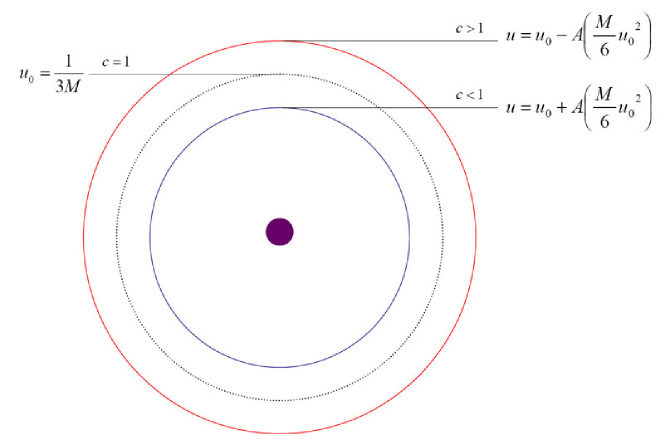
Figure 4.1: Orbit shifts about the classic critical orbit $u_{0}=1/3M$, with corresponding shifts in the speed of light (Not to scale)

.

4.2 Quantum Modified General Geodesics

Using the solutions for the critical circular orbits and the associated impact parameters we can now study how the general photon trajectories are modified due to quantum corrections. In the classic case when a photon comes in from infinity, with the critical impact parameter, it tends to the critical orbit, as was shown in Fig. 2.3; and if we slightly decrease the impact parameter the photon spirals into the singularity, Fig. 2.5. We will now construct a general quantum modified equation of motion and determine how the geodesics change, depending on polarization, as they tend to the critical orbits.

4.2.1 General Vectors

From the quantum modification term in Eqn. (4.1) we can see that in order to construct a general quantum modified geodesic equation we require general photon polarization and wave vectors. The wave vector, $k^{\mu}$, can no longer be represented by a simple constant vector pointing in the $\phi$ direction, as given in the orthonormal frame. And, even though the vertical polarization will remain a constant, as before, the planar polarization will now be a more general vector, constantly changing as the photon moves through the plane.

General Wave Vectors

Our general wave vector will be of the form:

$$k^{\mu}=(\frac{dt}{d\tau},\frac{dr}{d\tau},\frac{d\theta}{d\tau},\frac{d\phi}{d\tau})$$ (4.56)

which respects the light cone condition:

$$0=g_{\mu\nu}k^{\nu}k^{\mu}=F\dot{t}^{2}-F^{-1}\dot{r}^{2}-r^{2}\dot{\phi}^{2}$$ (4.57)

where $g_{\mu\nu}$ is the Schwarzschild metric. Using previous results, of Eqns (2.12) and (2.13), and the fact that we are working in the plane, $\theta=\frac{\pi}{2}$, we can represent three of the wave vector components as:

$$\frac{dt}{d\tau}=EF^{-1}\qquad\frac{d\phi}{d\tau}=\frac{J}{r^{2}}\qquad\frac{d\theta}{d\tau}=0$$ (4.58)

where we have defined:

$$F=(1-\frac{2M}{r})$$ (4.59)

Now using Eqn. (4.57) we can write the final component as:

$$(\frac{dr}{d\tau})^{2} = F^{2}(\frac{dt}{d\tau})^{2}-r^{2}F(\frac{d\phi}{d\tau})^{2}$$

$$\frac{dr}{d\tau} = \sqrt{E^{2}-\frac{J^{2}F}{r^{2}}}=E(1-\frac{D^{2}F}{r^{2}})^{\frac{1}{2}}$$ (4.60)

where we have used $D^{2}=\frac{J^{2}}{E^{2}}$. Now the general wave vector can be written as:

$$k^{\mu}=(EF^{-1},E(1-\frac{D^{2}F}{r^{2}})^{\frac{1}{2}},0,\frac{J}{r^{2}})$$ (4.61)

Also:

$$k_{\mu} = g_{\mu\nu}k^{\nu}$$

$$k_{\mu} = (E,-F^{-1}E(1-\frac{D^{2}F}{r^{2}})^{\frac{1}{2}},0,-J)$$ (4.62)

We now have:

$$k_{\mu}k^{\mu}=E^{2}F^{-1}-F^{-1}E^{2}(1-\frac{D^{2}F}{r^{2}})-\frac{J^{2}}{r^{2}}=0$$

as required. Therefore, eliminating $E$, we have the general wave vectors:

$$k^{\mu} = \frac{J}{D}(F^{-1},(1-\frac{D^{2}F}{r^{2}})^{\frac{1}{2}},0,\frac{D}{r^{2}})$$ (4.63)

$$k_{\mu} = \frac{J}{D}(1,-F^{-1}(1-\frac{D^{2}F}{r^{2}})^{\frac{1}{2}},0,-D)$$ (4.64)

We now need to normalize these vectors so, as they come in from infinity and tend to the critical circular orbit, they correspond to the critical orbit vector (4.8). However, as (4.8) is given in the orthonormal basis, and we are now working in the coordinate frame, we must use the tetrad (A.44), given in Appendix B, to transform (4.8) to its coordinate frame equivalent. Therefore, (4.8) in the coordinate basis is given as:

$$k^{\mu}=(e^{-1})^{\mu}_{a}k^{a}=(e^{-1})^{\mu}_{a}\left(\begin{array}[]{c}E_{k}\\ 0\\ 0\\ E_{k}\\ \end{array}\right)=E_{k}\left(\begin{array}[]{c}F^{-\frac{1}{2}}\\ 0\\ 0\\ \frac{1}{r}\\ \end{array}\right)$$ (4.65)

This now corresponds to a wave vector for a circular orbit in the coordinate frame. To represent the critical orbit we simply substitute for $r=3M$, in which case $F=1-\frac{2M}{r}\rightarrow\frac{1}{3}$, thus (4.65) becomes:

$$k^{\mu}=E_{k}(\sqrt{3},0,0,\frac{1}{3M})$$ (4.66)

Now, if we evaluate (4.64) with $r=3M$ and $D=3\sqrt{3}M$ we have:

$$k^{\mu}=\frac{J}{D}\sqrt{3}(\sqrt{3},0,0,\frac{1}{3M})$$ (4.67)

Therefore, (4.67) is similar to (4.66) up to a constant of normalization, given as:

$$E_{k}=\frac{J}{D}\sqrt{3}=E\sqrt{3}$$ (4.68)

Then, the normalized form of (4.64) is given by using (4.68):

$$k^{\mu}=\frac{E_{k}}{\sqrt{3}}(F^{-1},(1-\frac{D^{2}F}{r^{2}})^{\frac{1}{2}},0,\frac{D}{r^{2}})$$ (4.69)

General Polarization Vectors

Now we need to construct the, planar and vertical, polarization vectors, $a^{\mu}$, of the photon; which must be spacelike normalized as:

$$a_{\mu}a^{\mu}=-1\qquad a_{\mu}k^{\mu}=0$$ (4.70)

As before, as we are working in a plane, the vertical polarization, $a^{\mu}_{1}$, will be a constant, and can simply be written as:

$$a_{1}^{\mu}=(0,0,1,0)$$ (4.71)

To normalize this we do as follows:

$$a_{1\mu}=g_{\mu\nu}a^{\nu}_{1}=-r^{2}(0,0,1,0)\qquad\Rightarrow\qquad a_{1}^{\mu}a_{1\mu}=-r^{2}$$ (4.72)

Therefore, the normalized vertical polarization vector is given as:

$$a_{1}^{\mu} = (0,0,\frac{1}{r},0)$$

$$a_{1\mu} = -r^{2}(0,0,\frac{1}{r},0)$$ (4.73)

These now satisfy both the conditions in (4.70). The planar polarized vector, $a^{\mu}_{2}$, is given in the plane of $r$ and $\phi$:

$$a^{\mu}_{2}=(0,A,0,B)$$ (4.74)

Now, using the two conditions in (4.70) we can determine $A$ and $B$. From:

$$a_{2\mu}=g_{\mu\nu}a_{2}^{\nu}=(0,-AF^{-1},0,-r^{2}B)$$ (4.75)

and the vector (4.69) we have:

$$k^{\mu}a_{2\mu}=(1-\frac{D^{2}F}{r^{2}})^{\frac{1}{2}}(AF^{-1})+(\frac{D}{r^{2}})(r^{2}B)=0$$ (4.76)

$$a^{2\mu}a_{2\mu}=A^{2}F^{-1}+B^{2}r^{2}=-1$$ (4.77)

Solving these for $A$ and $B$:

$$B=-\frac{F^{-1}}{D}(1-\frac{D^{2}F}{r^{2}})^{\frac{1}{2}}A$$ (4.78)

$$A^{2}=\frac{F}{(1+\frac{r^{2}F^{-1}}{D^{2}}(1-\frac{D^{2}F}{r^{2}}))}$$ (4.79)

Therefore, we have:

$$A=\frac{DF}{r}\qquad B=-\frac{1}{r}(1-\frac{D^{2}F}{r^{2}})^{\frac{1}{2}}$$ (4.80)

and the planar polarization vector becomes:

$$a_{2}^{\mu}=(0,\frac{DF}{r},0,-\frac{1}{r}(1-\frac{D^{2}F}{r^{2}})^{\frac{1}{2}})$$ (4.81)

We now have the required polarization vectors:

$$a_{1}^{\mu} = \frac{1}{r}(0,0,1,0)$$ (4.82)

$$a_{1\mu} = -r^{2}(0,0,\frac{1}{r},0)$$ (4.83)

$$a_{2}^{\mu} = \frac{1}{r}(0,DF,0,-(1-\frac{D^{2}F}{r^{2}})^{\frac{1}{2}})$$ (4.84)

$$a_{2\mu} = (0,-\frac{D}{r},0,(1-\frac{D^{2}F}{r^{2}})^{\frac{1}{2}})$$ (4.85)

where subscript 1 and 2 are vertical and planar polarizations respectively. These now satisfy the conditions in (4.70) with the wave vector (4.69).

4.2.2 Quantum Modification

Having derived the general polarization and wave vectors, we can see from Eqn. (3.15) that the quantum modification given by:

$$\delta k(a)=\frac{8c_{\alpha}}{m_{e}^{2}}R_{abcd}k^{a}k^{c}a^{b}a^{d}$$ (4.86)

also requires the Riemann tensor components in the coordinate frame. In Appendix A we have calculated the required components as:

$$R^{\prime}_{trrt} = -\frac{2M}{r^{3}}\qquad R^{\prime}_{\theta rr\theta}=-\frac{MF^{-1}}{r}\qquad R^{\prime}_{\phi rr\phi}=-\frac{MF^{-1}}{r}$$

$$R^{\prime}_{\phi\theta\theta\phi} = 2Mr\qquad R^{\prime}_{\theta t\theta t}=-\frac{MF}{r}\qquad R^{\prime}_{\phi t\phi t}=-\frac{MF}{r}$$ (4.87)

Using this information we will now determine the form of the general quantum modification; and from the polarization rule, this quantum correction should satisfy the condition: $\delta k_{1}^{2}=-\delta k_{2}^{2}$ for the two polarizations.

For vertical $(\theta)$ polarization we have, by using (4.69) and (4.82) in (4.86):

$$R_{abcd}k^{a}k^{c}a_{1}^{b}a_{1}^{d} = R_{a\theta c\theta}\frac{1}{r^{2}}k^{a}k^{c}=R_{t\theta t\theta}\frac{1}{r^{2}}k^{t}k^{t}+R_{r\theta r\theta}\frac{1}{r^{2}}k^{r}k^{r}+R_{\phi\theta\phi\theta}\frac{1}{r^{2}}k^{\phi}k^{\phi}$$ (4.88)

$$= -\frac{MF}{r}(\frac{1}{r^{2}})(\frac{F^{-1}E_{k}}{\sqrt{3}})(\frac{F^{-1}E_{k}}{\sqrt{3}})$$

$$+ \frac{MF^{-1}}{r}(\frac{1}{r^{2}})(\frac{\sqrt{1-\frac{D^{2}F}{r^{2}}}E_{k}}{\sqrt{3}})(\frac{\sqrt{1-\frac{D^{2}F}{r^{2}}}E_{k}}{\sqrt{3}})$$

$$- 2Mr(\frac{1}{r^{2}})(\frac{DE_{k}}{r^{2}\sqrt{3}})(\frac{DE_{k}}{r^{2}\sqrt{3}})$$

$$= -\frac{ME_{k}^{2}F^{-1}}{3r^{3}}+\frac{ME_{k}^{2}F^{-1}(1-\frac{D^{2}F}{r^{2}})}{3r^{3}}-\frac{2ME_{k}^{2}D^{2}}{3r^{5}}$$

$$= -\frac{ME_{k}^{2}D^{2}}{r^{5}}$$

Similarly, for planar ($r-\phi$ plane) polarization we have, by using (4.69) and (4.84) in (4.86):

$$R_{abcd}k^{a}k^{c}a_{2}^{b}a_{2}^{d} = R_{arcr}k^{a}k^{c}a_{2}^{r}a_{2}^{r}+R_{arc\phi}k^{a}k^{c}a_{2}^{r}a_{2}^{\phi}+R_{a\phi cr}k^{a}k^{c}a_{2}^{\phi}a_{2}^{r}$$ (4.89)

$$+ R_{a\phi c\phi}k^{a}k^{c}a_{2}^{\phi}a_{2}^{\phi}$$

$$= R_{trtr}k^{t}k^{t}a_{2}^{r}a_{2}^{r}+R_{\phi r\phi r}k^{\phi}k^{\phi}a_{2}^{r}a_{2}^{r}+R_{\phi rr\phi}k^{\phi}k^{r}a_{2}^{r}a_{2}^{\phi}$$

$$+ R_{r\phi\phi r}k^{r}k^{\phi}a_{2}^{\phi}a_{2}^{r}+R_{t\phi t\phi}k^{t}k^{t}a_{2}^{\phi}a_{2}^{\phi}+R_{r\phi r\phi}k^{r}k^{r}a_{2}^{\phi}a_{2}^{\phi}$$

$$= \frac{2M}{r^{3}}(\frac{F^{-1}E_{k}}{\sqrt{3}})^{2}(\frac{DF}{r})^{2}+\frac{MF^{-1}}{r}(\frac{DE_{k}}{\sqrt{3}r^{2}})^{2}(\frac{DF}{r})^{2}$$

$$+ \frac{MF^{-1}}{r}(\frac{DE_{k}}{\sqrt{3}r^{2}})(\frac{E_{k}}{\sqrt{3}}\sqrt{1-\frac{D^{2}F}{r^{2}}})(\frac{DF}{r})(\frac{\sqrt{1-\frac{D^{2}F}{r^{2}}}}{r})$$

$$+ \frac{MF^{-1}}{r}(\frac{E_{k}\sqrt{1-\frac{D^{2}F}{r^{2}}}}{\sqrt{3}})(\frac{DE_{k}}{\sqrt{3}r^{2}})(\frac{\sqrt{1-\frac{D^{2}F}{r^{2}}}}{r})(\frac{DF}{r})$$

$$- \frac{MF}{r}(\frac{F^{-1}E_{k}}{\sqrt{3}})^{2}(\frac{\sqrt{1-\frac{D^{2}F}{r^{2}}}}{r})^{2}$$

$$+ \frac{MF^{-1}}{r}(\frac{E_{k}\sqrt{1-\frac{D^{2}F}{r^{2}}}}{\sqrt{3}})^{2}(\frac{\sqrt{1-\frac{D^{2}F}{r^{2}}}}{r})^{2}$$

$$= \frac{ME_{k}^{2}D^{2}}{r^{5}}$$

Therefore, the quantum modifications, $k^{2}=\delta k(a)$, for the two polarizations $a_{1}$ and $a_{2}$ (vertical and planar respectively) are:

$$\delta k(a_{1}) = -(\frac{8c_{\alpha}}{m_{e}^{2}})\frac{ME_{k}^{2}D^{2}}{r^{5}}\qquad\textrm{Vertical}$$ (4.90)

$$\delta k(a_{2}) = (\frac{8c_{\alpha}}{m_{e}^{2}})\frac{ME_{k}^{2}D^{2}}{r^{5}}\qquad\textrm{Planar}$$ (4.91)

where $-\delta k(a_{1})=\delta k(a_{2})$, as required. Now, using $k^{\mu}k_{\mu}-\delta k(a)$=0 we can write the general equations of motion for the two polarizations:

$$k^{\mu}k_{\mu}\pm(\frac{8c_{\alpha}}{m_{e}^{2}})\frac{ME_{k}^{2}D^{2}}{r^{5}}=0$$

$$(\frac{dr}{d\tau})^{2}=F^{2}(\frac{dt}{d\tau})^{2}-r^{2}F(\frac{d\phi}{d\tau})^{2}\pm F(\frac{8c_{\alpha}}{m_{e}^{2}})\frac{ME_{k}^{2}D^{2}}{r^{5}}$$

As before, substituting for $\dot{t}$, $\dot{\phi}$ and transforming $r\rightarrow\frac{1}{u}$, we have:

$$(\frac{du}{d\phi})^{2}=\frac{1}{D^{2}}-Fu^{2}\pm(\frac{D^{2}MA}{3})Fu^{5}$$ (4.92)

We can also write $u$ as a function of time:

$$(\frac{du}{dt})^{2}=(Du^{2}F)^{2}(\frac{1}{D^{2}}-Fu^{2}\pm(\frac{D^{2}MA}{3})Fu^{5})$$ (4.93)

where we have used the substitution for $A$ given in equation (4.31). Now, the Eqns. 4.92 and 4.93 are the general equations of motion, $+$ for vertical ($\theta$) polarization and $-$ for planar ($r$-$\phi$) polarization. In these equations we not only use the impact parameter of the form $1/D^{2}$ but also $D^{2}$, therefore the parameters for the two polarizations are given as:

$$\frac{1}{D^{2}}=\frac{u_{0}^{2}}{3}(1\pm AMu_{0})\rightarrow D=\frac{\sqrt{3}}{u_{0}}\mp\frac{\sqrt{3}AM}{2}+\mathcal{O}(A)$$ (4.94)

4.2.3 General Trajectory to the Critical Orbit.

Now that we have the general orbit equation (4.92) we can first test whether, for the critical impact perimeter $D$, the equation $\frac{du}{d\phi}\rightarrow 0$ for first order in $A$. Substituting the critical orbits and the impact parameters given in (4.54),(4.55) and (4.94) into (4.92) and expanding up to first order in $A$ we have: For planar polarization.

$$(\frac{du}{d\phi})^{2} = \frac{u_{0}^{2}}{3}(1+AMu_{0})-[1-2M(u_{0}(1+\frac{AM}{6}u_{0}))[(u_{0}(1+\frac{AM}{6}u_{0})]^{2}$$ (4.95)

$$- (\frac{\frac{3}{u_{0}^{2}(1+AMu_{0})}AM}{3})[1-2M[u_{0}(1+\frac{AM}{6}u_{0})]][u_{0}(1+\frac{AM}{6}u_{0})]^{5}$$

$$\rightarrow 0$$

and similarly for vertical polarization.

$$(\frac{du}{d\phi})^{2} = \frac{u_{0}^{2}}{3}(1-AMu_{0})-[1-2M[u_{0}(1-\frac{AM}{6}u_{0})]][u_{0}(1-\frac{AM}{6}u_{0})]^{2}$$ (4.96)

$$- (\frac{\frac{3}{u_{0}^{2}(1-AMu_{0})}AM}{3})[1-2[(u_{0}(1-\frac{AM}{6}u_{0})]][u_{0}(1-\frac{AM}{6}u_{0})]^{5}$$

$$\rightarrow 0$$

Expanding these and eliminating all terms of order $A^{2}$ and higher, we find that the right hand sides go to zero, as required. Thus for the appropriate impact parameters these equations behave as they should.

The next step is to solve equation (4.92) for the two polarizations. This is most simply done using numerical methods in Mathematica. As a guide, we know our solution will be of the form $u=u_{0}+ku_{1}$, where $u_{0}$ will be the classical solution (2.39), $u_{1}$ will be a small modification that pushes the critical orbit up or down depending on photon polarization, and $k$ will be some constant that is first order in $A$, i.e. of the form $k=As$, where $s$ will be some number given by the boundary condition: for $\phi\rightarrow\infty$ then $u(\phi)\rightarrow u_{0}(1\pm\frac{A}{6}u_{0})$. If we substitute for the critical impact parameter $D$ from (4.54) and (4.55) depending on the polarization, and then transform to $u\rightarrow u_{0}+Asu_{1}$, and expand to first order in $A$, we have non-linear first order differential equations in $u_{0}$, $u_{1}$ and $\phi$.

• For planar polarization:

  $$\frac{du_{1}(\phi)}{d\phi} = \frac{}{6s\sqrt{\frac{1}{27M^{2}}-u_{0}(\phi)^{2}+2Mu_{0}(\phi)^{3}}}[\frac{1}{27M^{2}}-27M^{3}u_{0}(\phi)^{5}$$ (4.97)

  $$+ 54M^{4}u_{0}(\phi)^{6}-6su_{0}(\phi)u_{1}(\phi)+18sMu_{0}(\phi)^{2}u_{1}(\phi)]$$

• For vertical polarization:

  $$\frac{du_{1}(\phi)}{d\phi} = \frac{1}{6s\sqrt{\frac{1}{27M^{2}}-u_{0}(\phi)^{2}+2Mu_{0}(\phi)^{3}}}[-\frac{1}{27M^{2}}+27M^{3}u_{0}(\phi)^{5}$$ (4.98)

  $$- 54M^{4}u_{0}(\phi)^{6}-6su_{0}(\phi)u_{1}(\phi)+18sMu_{0}(\phi)^{2}u_{1}(\phi)]$$

These can be solved in one of two ways, (i) is to substitute the classic solution (2.39) for $u_{0}$ and solve analytically, (ii) is to solve $\frac{du_{1}}{d\phi}$ and the classic equation for $\frac{du_{0}}{d\phi}$ simultaneously using numerical techniques. We attempted to use method (i) to derive an analytic solution for $u_{1}(\phi)$, however, due to the complex nature of the equation we proceeded to use method (ii), that is solving by numerical methods. To do this we set the constant $s=1$, and then when the numerical values of $u_{1}(\phi)$ were determined we could determine the constant $s$ so that $u(\phi)$ coincided with the modified circular orbits given in (4.54) and (4.55). This technique was used for reasons of convenience, because solving (4.97) and (4.98) for various values of $s$ would be time consuming as each numerical calculation takes a significant amount of time; therefore solving them once and then scaling the solution is a more convenient method. The results of the equations were plotted as:

$$u(\phi)=u_{0}(\phi)+Asu_{1}(\phi)$$ (4.99)

where the constant $s$ was picked to satisfy the condition: $\phi\rightarrow\infty$ $\Rightarrow$ $u(\phi)\rightarrow u_{0}(1\pm\frac{A}{6}u_{0})$ i.e. the trajectories tend to the critical orbit, depending on polarization. In this way the constant $s$ was determined to be $s=1/3$, which was tested for various values of $M$. We have plotted the results of the numerical calculation in Figs. 4.2 and 4.3. In Fig. 4.2, you can see that the general critical orbits follow a classic style path, however the orbit splitting is not clearly visible. But in Fig. 4.3 we have plotted a closer view of the critical orbits, and here the splitting is highly visible. It can be seen that the general trajectories for the planar and vertically polarized photons tend to the relevant critical orbits.

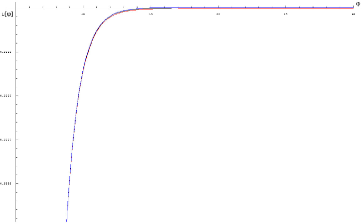
Figure 4.2: The quantum modified critical orbits follow classic type paths. We have used a factor $A=0.00009$ in order to make the quantum corrections more visible, where a real value should be of order $\sim 10^{-32}$, Eqn. 4.38. The splitting of the orbits can be clearly seen in the Fig. 4.3, given below.

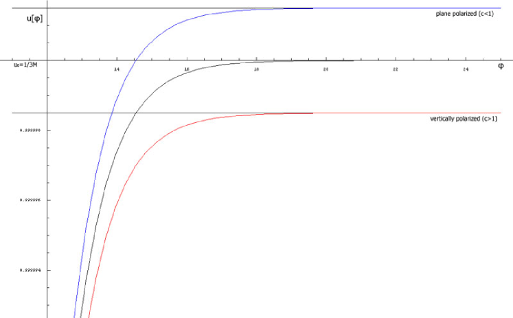
Figure 4.3: The quantum modified trajectories show clear splitting as they tend to the critical points. We used the constants $M=\frac{1}{3}$ and $A=0.00009$.

4.3 Quantum Modification and the Event Horizon

In Chapter. 2 it was shown that when we decreased the impact parameter from the critical value ($D=3\sqrt{3}M$ to $D-1/10$) the photon trajectory, given as $u(\phi)$, spiraled into the singularity, Fig. 2.5; and when we represent the trajectory as a function of coordinate time, $u(t)$, it tends to the event horizon, $u=1/2M$. From the horizon theorem it was seen that quantum modifications have no effect on photon velocities directed normal to the event horizon. So this implies when a photon tends to the event horizon at an angle, e.g. with an impact parameter $D=D_{critical}-1/10$, then the component of velocity normal to the horizon should be unchanged, while the component parallel to it is modified according to the quantum correction; this modification should then result in a shift of the photon trajectory, but the horizon should remain fixed. In order to test this we used Eqn. (4.92) with an impact parameter $D=D_{critical}-1/10$ to show that the photon trajectories still fall into the singularity. We then used Eqn. (4.93), with the new impact parameter, to study the behavior of the trajectories around the event horizon.

4.3.1 Trajectories to the singularity

In order to construct quantum modified trajectories, which go past the critical orbit and fall into the singularity, we require the impact parameters:

$$\frac{1}{D^{2}}=\frac{1}{(\frac{\sqrt{3}}{u_{0}\sqrt{(1\pm AMu_{0})}}-\frac{1}{10})^{2}}\rightarrow D=\frac{\sqrt{3}}{u_{0}}\mp\frac{\sqrt{3}AM}{2}-\frac{1}{10}+\mathcal{O}(A)$$ (4.100)

where, as before, $+$ is for vertical polarization and $-$ is planar polarization, in $1/D^{2}$. For these impact parameters we numerically solved Eqn. (4.92), and in Fig. 4.4 we can see that all the trajectories follow a classic type path into the singularity. However, near the singularity you can see the splitting of the orbits as they tend to $u\rightarrow\infty$. In Fig. 4.5 we have shown a magnified view of the point where the trajectories cross the event horizon. In this figure it can be seen that the planar polarized photon ($c<1$) crosses the event horizon at a point before the classic trajectory and the vertically polarized photon ($c>1$) crosses it at a point after the classic trajectory. This makes sense, as the planar polarized photons are pushed towards the black hole and vertically polarized trajectories are pushed out, the vertically polarized ones must spiral further around the black hole to reach the event horizon compared to the classic or the planar polarized trajectories.

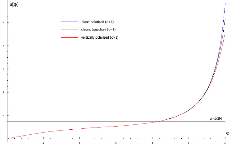
Figure 4.4: The quantum modified trajectories follow similar paths, as the classic trajectory, to the singularity, with $M=\frac{1}{3}$ and $A=0.0009$.

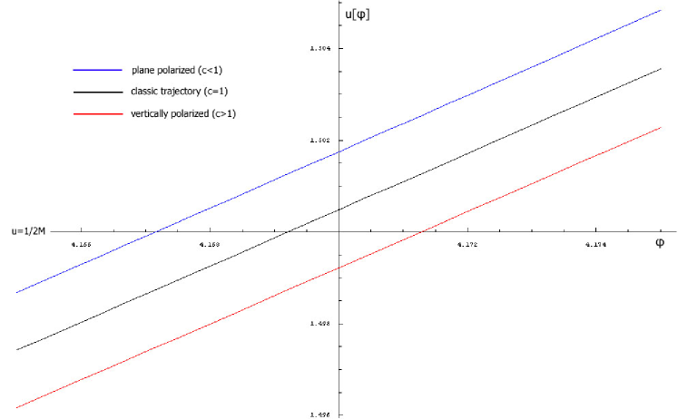
Figure 4.5: The classic and quantum modified trajectories crossing the event horizon $u=2M$, with $M=\frac{1}{3}$ and $A=0.0009$.

4.3.2 Fixed Event Horizon

To demonstrate the fact that the event horizon remains fixed at $u=1/2M$ we applied the impact parameters given by (4.100) to Eqn.(4.93). Again, solving numerically we found that the trajectories tend to the event horizon in the classic way, Fig. 4.6, however, they are again slightly shifted. In Fig. 4.7, a close up of the point where the trajectories tend to the event horizon at $u=1/2M$, you can clearly see that the quantum modified orbits tend to the horizon before the classic orbit. This can be understood by the fact that the planar polarized trajectory is pushed towards the black hole, hence it has less of a distance to propagate before it reaches the horizon, and even though the vertically polarized trajectory is pushed outwards, the fact that it has a faster velocity than $c=1$ it reaches the event horizon before the classic trajectory.

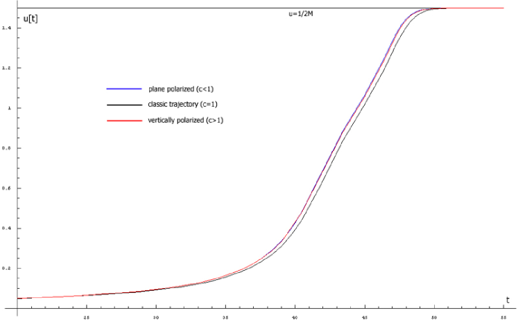
Figure 4.6: The quantum modified trajectories follow similar paths, as the classic trajectory, to the event horizon, with $M=\frac{1}{3}$ and $A=0.0009$.

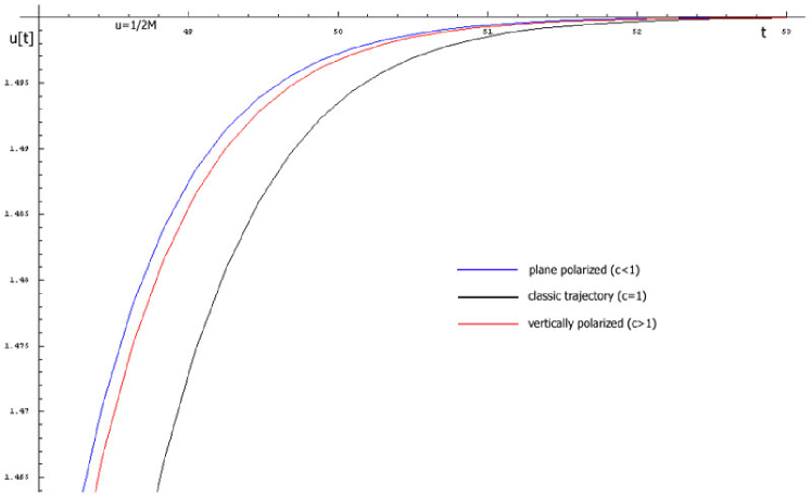
Figure 4.7: The classic and quantum modified trajectories reach the event horizon at differing times, with $M=\frac{1}{3}$ and $A=0.0009$.

The other more important thing we can note from this calculation is that the event horizon remains fixed at the classic point $u=1/2M$, due to the fact that, as was stated earlier, the quantum correction has no effect on photon momentum normal to the horizon. This means even though the quantum correction implies velocities greater than the speed of light, no photons can escape from the event horizon, so the black hole remains black.

Chapter 5 Quantum Modified Schwarzschild Metric

Now, using our previous results, we can construct a new metric that encompasses the quantum corrections due to vacuum polarization. This metric should then be a sum of the classic Schwarzschild metric and the polarization dependent quantum corrections we derived in Eqns. (4.88) and (4.89):

$$\mathcal{G}_{\mu\nu}k^{\mu}k^{\nu} = (g_{\mu\nu}+\mathfrak{g}_{\mu\nu})k^{\mu}k^{\nu}=0$$ (5.1)

$$= (g_{\mu\nu}-\frac{8c_{\alpha}}{m_{e}^{2}}R_{\mu\eta\nu\lambda}a^{\eta}a^{\lambda})k^{\mu}k^{\nu}=0$$

5.1 Construction of the Metric

Using the results in Sec. 4.2.2 we can write the first components of the quantum modified metric $\mathcal{G}_{tt}^{1}$ and $\mathcal{G}_{tt}^{2}$, for vertical and planar polarization respectively, as:

$$\mathcal{G}_{tt}^{1} = g_{tt}-\frac{8c_{\alpha}}{m_{e}^{2}}R_{tbtd}a_{1}^{b}a_{1}^{d}$$ (5.2)

$$= F-\frac{8c_{\alpha}}{m_{e}^{2}}(-\frac{MF}{r})(\frac{1}{r^{2}})$$

$$= F+\frac{AMD^{2}}{9}Fu^{3}$$

$$\mathcal{G}_{tt}^{2} = g_{tt}-\frac{8c_{\alpha}}{m_{e}^{2}}R_{tbtd}a_{2}^{b}a_{2}^{d}$$ (5.3)

$$= F-\frac{8c_{\alpha}}{m_{e}^{2}}[\frac{2M}{r^{3}}(\frac{DF}{r})^{2}-(\frac{MF}{r})(\frac{\sqrt{1-\frac{D^{2}F}{r^{2}}}}{r})^{2}]$$

$$= F-\frac{AMD^{2}}{9}(3D^{2}F^{2}u^{5}-Fu^{3})$$

where, in the last lines of each component, we have used Eqn (4.31) to replace the constants with $A$, and we’ve made the transformation $r\rightarrow 1/u$. Now, doing this for all the other components we can construct the metrics for vertical and planar polarizations:

• Vertical Polarization: $a_{1}^{\mu}=u(0,0,1,0)$

  $$\mathcal{G}^{1}_{\mu\nu}=\left(\begin{array}[]{cccc}F-BFu^{3}&0&0&0\\ 0&-\frac{1}{F}+\frac{Bu^{3}}{F}&0&0\\ 0&0&-\frac{1}{u^{2}}&0\\ 0&0&0&-\frac{1}{u^{2}}-Bu\\ \end{array}\right)$$ (5.4)

• Planar Polarization: $a_{2}^{\mu}=u(0,DF,0,D\frac{du}{d\phi})$

  $$\mathcal{G}^{2}_{\mu\nu}=\left(\begin{array}[]{cccc}F+BFu^{3}(1-3D^{2}Fu^{2})&0&0&0\\ 0&-\frac{1}{F}-\frac{Bu^{3}(1-D^{2}Fu^{2})}{F}&0&Bu^{3}D\frac{du}{d\phi}\\ 0&0&-\frac{1}{u^{2}}&0\\ 0&Bu^{3}D\frac{du}{d\phi}&0&-\frac{1}{u^{2}}-BD^{2}Fu^{3}\\ \end{array}\right)$$ (5.5)

where $B=\frac{AMD^{2}}{9}$. These are now the relevant quantum modified Schwarzschild metrics for vertical and planar polarizations.

5.2 Dynamics with the Quantum Modified Metric

We can now derive the same equations of motion as (4.92), but now we can do it simply with the quantum modified metrics. Using the general wave vector in a plane:

$$k^{\mu} = (\dot{t},\dot{r},\dot{\theta},\dot{\phi})$$ (5.6)

$$= (\frac{J}{D}F^{-1},-J\frac{du}{d\phi},0,Ju^{2})$$

where we have transformed to $r\rightarrow 1/u$, and we substitute for $\dot{t}$ and $\dot{\phi}$ as before. Applying this wave vector to (5.4) and(5.5) we find:

$$0 = \mathcal{G}^{1}_{\mu\nu}k^{\mu}k^{\nu}$$ (5.7)

$$\Rightarrow (\frac{du}{d\phi})^{2}=\frac{1}{D^{2}}-Fu^{2}+(\frac{D^{2}A}{3})Fu^{5}$$

for vertical polarization, and

$$0 = \mathcal{G}^{2}_{\mu\nu}k^{\mu}k^{\nu}$$ (5.8)

$$\Rightarrow (\frac{du}{d\phi})^{2}=\frac{1}{D^{2}}-Fu^{2}-(\frac{D^{2}A}{3})Fu^{5}$$

for planar polarization. These are identical to the equations we derived in Sec. 4.2.2.

Radial Geodesics

We can now show that the metric for vertical polarization is consistent with the fact that radially projected photon trajectories are not modified. By using the vertical polarization metric, (5.4), and a general radial wave vector, ($k^{\mu}=(\dot{t},\dot{r},0,0)$, we find:

$$0 = \mathcal{G}^{1}_{\mu\nu}k^{\mu}k^{\nu}$$

$$\Rightarrow\qquad\frac{dt}{dr} = \pm\frac{1}{F}$$ (5.9)

which is identical to the classic radial geodesic equation, (2.30). However, the same is not true for the planar polarization metric. Due to our derivation of the polarization vectors in Sec. 4.2.1, we constructed a very general vertical polarization vector and then normalized it; however, the one for planar polarization was constructed for the case where $\frac{d\phi}{d\tau}\neq 0$, as can be seen in Eqns. (4.60) and (4.76); therefore the planar polarization vector has $\phi$ dependence "mixed" into it through the substitution of $\dot{\phi}$:

$$(\frac{dr}{d\tau})^{2} = F^{2}(\frac{dt}{d\tau})^{2}-r^{2}F(\frac{d\phi}{d\tau})^{2}$$

$$= (E^{2}-\frac{J^{2}F}{r^{2}})^{\frac{1}{2}}=E(1-\frac{D^{2}F}{r^{2}})^{\frac{1}{2}}$$

We can note that it’s a result of the substitution $\frac{d\phi}{d\tau}=\frac{J}{r^{2}}$, in the polarization vectors, that we acquire an extra parameter $D$ in our quantum correction (apart from the one introduced through normalization, which was incorporated into $B=AD^{2}/9$). We can then say that if we need to use the metric for a radial trajectory with $\frac{d\phi}{d\tau}=0$ we can just set $D=0$, as this would lead to the removal of the $\phi$ dependence. In this way, the planar polarized quantum modified metric for radial trajectories is:

$$\mathcal{G}(\textsl{$\phi$=0})^{2}_{\mu\nu}=\left(\begin{array}[]{cccc}F+BFu^{3}&0&0&0\\ 0&-\frac{1}{F}-\frac{Bu^{3}}{F}&0&0\\ 0&0&-\frac{1}{u^{2}}&0\\ 0&0&0&0\\ \end{array}\right)$$ (5.11)

Then applying this to a general radial wavevector, we again find the classic radial geodesic equation:

$$0 = \mathcal{G}(\textsl{$\phi$=0})^{2}_{\mu\nu}k^{\mu}k^{\nu}$$

$$\Rightarrow\qquad\frac{dt}{dr} = \pm\frac{1}{F}$$ (5.12)

Therefore, we have metrics for the Schwarzschild space time that incorporate quantum corrections due to vacuum polarization; and these metrics are consistent with classic results.

Chapter 6 Summary

For Schwarzschild Spacetime we showed, in the orthonormal frame, that, due to quantum corrections, the stable circular orbit at $u_{0}=1/3M$ splits depending on the polarization of the photon, and the new modified circular orbits are given by the classical orbit plus a correction term to first order in a dimensionless constant $A$: $u=u_{0}+Au_{1}$, where $A=\frac{24c_{\alpha}E_{k}^{2}}{J^{2}m_{e}^{2}}$ and has an order of $10^{-32}$. As stated by the polarization sum rule this splitting of the critical orbit is equal in magnitude but opposite in sign for the two polarizations. We found that the vertically polarized photon (c>1) is pushed out by a correction of $u_{1}=-\frac{M}{6}u_{0}^{2}$, while the planar polarized photon is pulled in by a correction of $u_{1}=\frac{M}{6}u_{0}^{2}$. It was also found that this orbit shift also requires an appropriate modification of the classic impact parameter $\frac{1}{D_{0}^{2}}=\frac{u_{0}^{2}}{3}$. This modification, for the quantum corrected orbits, took the form $\frac{1}{D^{2}}=\frac{1}{D_{0}^{2}}+AD_{1}$, and again as for the orbit shift, the change was equal in magnitude but opposite in sign for the two polarizations: $D_{1}=\frac{Mu_{0}^{3}}{3}$ for planar polarization and $D_{1}=-\frac{Mu_{0}^{3}}{3}$ for vertical polarization. Using this information, for the splitting of circular orbits, we then constructed the quantum corrected general equations of motion for the Schwarzschild spacetime. Using these equation of motion it was shown that a photon starting at $u=0$, with the appropriate critical impact parameter, tends to the critical orbit associated with that impact parameter - and the trajectory follows a similar path to the classic case.

We then went on to show that, using the general quantum corrected equations of motion, a photon projected towards the black hole with an impact parameter less than the critical value falls into the the singularity, in terms of the angular distance ($\phi$). Although the photons follow a classic type path into the singularity, the trajectories are slightly shifted according to polarization. The planar polarized photon crosses the horizon before the classic trajectory, and the vertically polarized one crosses it after, this corresponds to the fact that planar polarized photons are pulled towards the black hole and vertically polarized ones are pushed away, hence the vertically polarized ones need to go a further angular distance to reach the event horizon.

In terms of coordinate time ($t$) we found that the photon trajectories tend to the event horizon. Therefore, the quantum corrections do not shift the classic event horizon from $u=\frac{1}{2M}$, which corresponds to the horizon theorem. Also, we found that, although the quantum corrected orbits follow a classic type path to the event horizon, the point at which they hit the horizon is, again, slightly shifted depending on polarization. However, this time both polarizations hit the horizon before the classic trajectory. The planar polarized photon tends to arrive at the horizon first, then the vertically polarized one, and finally the classic photon. This could correspond to the fact that the planar polarized photon, although it has a velocity lower than the speed of light, has less of a distance to go, as its trajectory is pulled towards the black hole. For the vertically polarized case, even though it has a faster than light velocity, it has a further distance to go to reach the horizon as its trajectory is pushed away from the black hole.

Having determined the equations of motion, with the quantum correction, we then went on to construct a Schwarzschild metric that incorporates the quantum correction: $\mathcal{G}_{\mu\nu}=(g_{\mu\nu}+\mathfrak{g}_{\mu\nu})$, where the correction: $\mathfrak{g}_{\mu\nu}$ was again first order in $A$. We showed that with this metric and a general photon wave vector, $k^{\mu}$, we obtain the quantum modified equations of motion, as before. Also, this new metric confirms the horizon theorem, that is, when we use a wave vector indicating a radially projected photon we obtain the classic equation of motions. This was fine for vertical polarization, however, in the planar polarization case we had a problem; we had previously used a substitution that mixed a "hidden" radial angle, $\phi$, into our polarization vector (as in general orbits the planar polarization depends on $\phi$). By tracing back to the origin of this substitution we found that, in order to study radial trajectories, we need to set $D=0$, this then removes the $\phi$ dependency; this then gives us the classic equation of motion for planar polarized radially projected photons.

So in conclusion, after studying the dynamics of null trajectories in Schwarzschild spacetime we derived the polarization dependent photon trajectories to first order in the constant $A$ (which is dependent on the fine structure constant, the mass of the star, mass of the electron, and the energy of the photon). We then incorporated these modification into a general quantum modified metric, which could also be used to derive the general quantum modified equations of motion. Also, the results of this work coincide with the conditions of the horizon theorem and the polarization sum rule.

Part II Superfluid Behaviour of the 2+1d NJL Model at High Density

Chapter 7 Introduction

7.1 Quantum Chromodynamics

Since the 70’s it has been accepted that nucleons and other hadrons (baryons and mesons) observed in particle accelerators are not fundamental particles themselves, but are composed of fractionally charged fermions known as quarks, which exchange bosons of the strong force known as gluons. In this description, known as the quark model, baryons and mesons are depicted as bound states of three quarks and quark anti-quark pairs respectively. In this way the quark model provides a very natural explanation for the multiplicity and pattern of all the strongly-interacting particles [13, 15]. Experimental tests of this theory (in a similar way to the classic high-angle Rutherford scattering of $\alpha$-particles off atoms demonstrating the existence of the nucleus) consists of high energy inelastic scattering experiments of electrons off nucleons. The evidence from such experiments is consistent with the presence of pointlike spin-$\frac{1}{2}$ constituents called partons with a mass one third that of the proton. These partons, which are able to move freely within the nucleon volume, are then identified with quarks.

7.1.1 QCD: A Model of Strongly Interacting Matter

Quantum Chromodynamics (QCD) was introduced in the early 70s as the theoretical framework that translated the experimental and conceptual description of the quark model into a quantitative calculational scheme. QCD describes quarks and anti-quarks as quanta of the elementary fermion fields $\psi$ and $\bar{\psi}$, each with an $SU(3)$ colour charge, and gluons as quanta of a self-interacting non-abelian gauge field $A_{\mu}$. The Lagrangian density of QCD is given by

$$\mathcal{L}_{QCD}=\bar{\psi}^{\alpha}_{i}(iD/\hskip 1.99997pt-m_{0})^{\alpha\beta}_{ij}\psi^{\beta}_{j}-\frac{1}{4}\mathcal{F}^{a}_{\mu\nu}\mathcal{F}_{a}^{\mu\nu}$$ (7.1)

In the fermionic part $i$ and $j$ run over $N_{f}$ flavours of quarks, $\alpha$ and $\beta$ run over the 3 colours, then $m_{0}$ is an $N_{f}\times N_{f}$ mass matrix in flavour space. The covariant derivative

$$D/\hskip 1.99997pt=\gamma^{\mu}D_{\mu}^{\alpha\beta}=\gamma^{\mu}(\delta^{\alpha\beta}\partial_{\mu}-\frac{i}{2}g(\lambda^{a})^{\alpha\beta}A^{a}_{\mu})$$ (7.2)

is introduced so the Lagrangian density is invariant under local $SU(3)$ gauge transformations, where $g$ is the bare coupling constant, $A^{a}_{\mu}$ is a vector (gauge) field with eight gluonic degrees of freedom and $\lambda^{a}$ denote the generators of the $SU(3)$ group. Due to the introduction of the eight gluon fields, through gauge symmetry, we adjoin the free gluon lagrangian (the final (gauge) part of the action) to give the full QCD lagrangian. In the free gluon term of the action the field strength tensor is

$$\mathcal{F}^{a}_{\mu\nu}=\partial_{\mu}A^{a}_{\nu}-\partial_{\nu}A^{a}_{\mu}+gf_{abc}A^{b}_{\mu}A^{c}_{\nu}$$ (7.3)

where $f_{abc}$ are the structure constants of the $SU(3)$ group. As the QCD lagrangian is symmetric under a non-Abelian gauge group, underlined by the presence of the structure constants $f^{abc}$, the theory has some non-trivial features that are not present in Abelian gauge theories like quantum electrodynamics[11]:

• $\mathcal{L}_{QCD}$ contains gluonic self-coupling (three and four gluon vertices), which means the gluons themselves carry colour.

• At large momentum, $Q$, the QCD coupling behaves as:

  $$\alpha_{s}\sim\frac{1}{\ln(Q^{2}/\Lambda^{2}_{QCD})}$$ (7.4)

  where $\Lambda_{QCD}\sim 200MeV$ is the QCD scale parameter.

• Eqn. (7.4) implies that $\alpha_{s}(Q^{2})\rightarrow 0$ as $Q^{2}\rightarrow\infty$, and $\alpha_{s}(Q^{2})\rightarrow\infty$ when $Q^{2}=\Lambda^{2}_{QCD}$.

This behaviour of the strong force is known as asymptotic freedom, and can be simply represented through the quark anti-quark potential

$$V(r)=-\frac{\alpha_{s}(r)}{r}+Kr$$ (7.5)

where $K$ is an experimentally determined constant, called the string tension, with an estimated value of $\simeq(420MeV)$[13]; and $\alpha_{s}$ is the coupling given in Eqn. (7.4), which varies with distance as $1/\ln(r^{-1})$. Now it can be seen that for small distances the first term dominates, in which case the strong force behaves like an attractive Coulomb potential, and in the limit $r\rightarrow 0$ the quarks can be considered as free non-interacting particles[13]. However, with greater separations the potential scales approximately linearly due to the self interaction of the gluons, as seen through the second term. This is related to the phenomenon of "confinement", i.e. to the empirical fact that coloured objects, like quarks and gluons, do not exist as physical degrees of freedom in the vacuum. So, as the coupling constant (related to the potential) becomes larger for greater separations perturbative treatments of QCD become less and less effective.

7.1.2 Lattice QCD

A perturbative treatment of QCD leads to a successful description of the force between quarks at small distances . However, as already stated, at large distances a perturbative treatment of QCD is less fruitful. One method to address the non-perturbative nature of QCD at large distances is that of Lattice Gauge Theory, proposed by Wilson in 1974. In this method all the fields are defined on a discrete Euclidean space-time lattice with a nonzero lattice spacing $a$. Thus, in this way the lattice QCD calculations can be numerically carried out without the use of perturbative expansion. Even with its advantages, lattice field theory still has problem, such as:

• It’s difficult to discretise the fermion field in a chirally symmetric way.

• Simulations with reasonable light current quark masses are computationally very expensive.

• To simulate a smooth space time by implementing a large lattice volume and small lattice spacing requires a very large number of lattice sites.

• Simulations for non-zero chemical potential ($\mu\neq 0$) are next to impossible due to the sampling weight (used in Monte-Carlo methods) becoming complex (Appendix C.1).

However, with the continual improvement of lattice algorithms and the advances in computing power, lattice QCD is the driving force in our understanding of strongly interacting matter.

7.2 Chiral Symmetry in QCD

An important feature of QCD is its chiral symmetry for fermions with a vanishing mass (or approximate symmetry as is the case for physical quarks). Chiral symmetry is related to the symmetries associated with a particle’s handedness, which in turn is defined by its helicity. Before we go into chiral symmetry we’ll briefly discuss the concept of helicity and chirality.

7.2.1 Helicity and Chirality

A particle propagating with spin $\vec{s}$ has helicity $h=\vec{s}\cdot\vec{k}/|k|$, which is the projection of the spin axis along the direction of its motion $\vec{k}$, where positive helicity is right-handed and negative is left-handed. Also, if the particle has a vanishing mass its helicity would then be invariant under Lorentz transformations, which (for the massless case) leads to two good quantum numbers $B_{L}$ and $B_{R}$, referring to the separate conservation of left- and right-handed particle numbers in the absence of external effects. However, in the case of massive particles these quantum numbers are not separately conserved, but their sum is a good quantum number: $B=B_{L}+B_{R}$. So, through this concept of helicity we can define the chirality operators that project out left- and right-handed field states

$$\psi_{L} = \frac{1}{2}(1-\gamma_{5})\psi=P_{L}\psi\qquad\psi_{R}=\frac{1}{2}(1+\gamma_{5})\psi=P_{R}\psi$$

$$\bar{\psi}_{L} = \bar{\psi}\frac{1}{2}(1+\gamma_{5})=\bar{\psi}P_{R}\qquad\bar{\psi}_{R}=\bar{\psi}\frac{1}{2}(1-\gamma_{5})=\bar{\psi}P_{L}$$ (7.6)

and these chiral field states, $\psi_{L}$ and $\psi_{R}$, satisfy the equations

$$\gamma_{5}\psi_{L}=-\psi_{L}\qquad\gamma_{5}\psi_{R}=+\psi_{R}$$ (7.7)

where $\gamma_{5}=i\gamma^{0}\gamma^{1}\gamma^{2}\gamma^{3}$ and its eigenvalues are called "chirality". In general, unlike helicity, chirality is not directly measurable. We find that in the limit where $m\rightarrow 0$ (or for $E\gg m$) the helicity and chirality of a particle are in one-to-one correspondence, and the chiral fields associated with the massless particles thus represent physical states. However, as helicity is not Lorentz invariant massive particle fields must be expressed as a sum of left- and right-handed chiral fields,

$$\psi=P_{L}\psi+P_{R}\psi=\psi_{L}+\psi_{R}$$ (7.8)

which is the covariant formulation of massive particles. So in this case, of massive particles, chirality and helicity are distinct things, and thus the chiral states are not physical states, but represent internal degrees of freedom.

7.2.2 Chiral Symmetry

With this discussion of handedness and chirality we can go on to discuss what is meant by chiral symmetry. In general, chiral symmetry is the symmetry associated with the independent transformations of the left- and right-handed chiral states of a particle. So, when we say QCD, for $N_{f}$ quark flavours, possesses chiral symmetry under $SU(N_{f})_{L}$ $\times$ $SU(N_{f})_{R}$, we actually refer to the lagrangian of the theory being invariant for the separate transformations of the left and right-handed chiral fields[19]

$$\psi \rightarrow V\psi,\qquad V=V_{L}P_{L}+V_{R}P_{R},$$ (7.9)

$$\bar{\psi} \rightarrow\bar{\psi}\bar{V},\qquad\bar{V}=V^{{\dagger}}_{L}P_{R}+V^{{\dagger}}_{R}P_{L}$$

where $V_{L}$, $V_{R}$ $\in$ $SU(N_{f})$. This is equivalent to the symmetry under the $SU(N_{f})_{V}\times SU(N_{f})_{A}$, with the transformations

$$SU(N_{f})_{V}: \psi\rightarrow e^{-\frac{i}{2}\tau_{a}\theta_{a}}\psi\qquad\bar{\psi}\rightarrow\bar{\psi}e^{\frac{i}{2}\tau_{a}\theta_{a}}$$

$$SU(N_{f})_{A}: \psi\rightarrow e^{-\frac{i}{2}\gamma_{5}\tau_{a}\vartheta_{a}}\psi\qquad\bar{\psi}\rightarrow\bar{\psi}e^{-\frac{i}{2}\gamma_{5}\tau_{a}\vartheta_{a}}$$

where $\tau_{a}$ are the generators of flavor $SU(N_{f})$. Chiral symmetry would be exact in the limit of $N_{f}$ massless flavours, but for non-vanishing mass ($m_{0}\neq 0$) it is explicitly broken from $SU(N_{f})_{V}\times SU(N_{f})_{A}$ to $SU(N_{f})_{V}$, as the mass term in $\mathcal{L}_{QCD}$ mixes the chiral states $\psi_{L}$ and $\psi_{R}$[16]. However, though quarks have non-vanishing masses, chiral symmetry is still a useful concept for the up/down quarks $(N_{f}=2)$ as the masses are very small and could be considered negligible compared to the QCD scale parameter $\Lambda_{QCD}$ (and to a lesser extent for the inclusion of the strange quark i.e. $N_{f}=3$). Thus, as long as the masses are small compared to the relevant scale of the theory one may treat $SU(N_{f})_{A}$ as an approximate symmetry, so that predictions based upon the assumptions of the symmetry should be reasonably close to the actual results[16]. As this is an approximate symmetry we could ask: what are the observable phenomena related to chiral symmetry being approximate rather than an exact symmetry? One of the most obvious effects is seen through the non-zero (but small) mass of the pions, i.e. the Goldstone bosons associated with the spontaneous breaking of chiral symmetry for $N_{f}=2$ (which will be discussed in the next section).

Total Chiral Symmetry Group of QCD

It can be shown that the QCD Lagrangian is also invariant under phase transformations of the left- and right-handed quarks ($u_{L}$ and $d_{L}$), which is the $U(1)_{L}\times U(1)_{R}$ symmetry. So the total chiral symmetry group of the QCD Lagrangian for $N_{f}=2$ flavors can be written as

$$U(2)_{L}\times U(2)_{R} = SU(2)_{L}\times SU(2)_{R}\times U(1)_{L}\times U(1)_{R}$$

$$= SU(2)_{V}\times SU(2)_{A}\times U(1)_{V}\times U(1)_{A}$$

where the axial and vector $U(1)$ rotations can be written as

$$U(1)_{V}: \psi\rightarrow e^{-i\theta}\psi\qquad\bar{\psi}\rightarrow\bar{\psi}e^{i\theta}$$

$$U(1)_{A}: \psi\rightarrow e^{i\gamma_{5}\vartheta}\psi\qquad\bar{\psi}\rightarrow\bar{\psi}e^{i\gamma_{5}\vartheta}$$

Having the full chiral symmetry group of QCD we can discuss the physical manifestations of theses symmetries in nature. The $U(1)_{A}$ symmetry is (said to be) explicitly broken due to quantum fluctuations[21], but the $U(1)_{V}$ symmetry is responsible for baryon number conservation, and hence is labeled as $U(1)_{B}$. The pure unitary transformation $SU(2)_{V}$ corresponds to isospin conservation, where the axial transformation, $SU(2)_{A}$, alters the parity that is associated with a state. This means the manifestation of $SU(2)_{A}$ in nature would require that each isospin multiplet be accompanied by a mirror multiplet that has opposite parity. However, as no such multiplets are observed in nature it is an accepted view that $SU(2)_{A}$ is a broken symmetry of QCD, where the resulting massless Goldstone bosons are associated with the pions. We can also write the conserved currents associated with each of the symmetries (as given by Klevansky [22]):

$$SU(2)_{V} : \qquad I^{k}_{\mu}=\bar{\psi}\gamma_{\mu}\tau^{k}\psi\Rightarrow Isospin$$

$$U(1)_{V} : \qquad I_{\mu}=\bar{\psi}\gamma_{\mu}\psi\Rightarrow Baryonic$$

$$SU(2)_{A} : \qquad I^{k}_{5\mu}=\bar{\psi}\gamma_{\mu}\gamma_{5}\tau^{k}\psi\Rightarrow Chiral$$

$$U(1)_{A} : \qquad I_{5\mu}=\bar{\psi}\gamma_{\mu}\gamma_{5}\psi\Rightarrow Axial$$

(7.13)

We have used the notation $I$ for the currents, this is due to the fact that in this thesis $J$ is reserved for source terms, as is the convention in condensed matter physics.

7.2.3 The QCD Vacuum and Spontaneous Symmetry Breaking

As discussed, due to the smallness of the current quark masses, QCD is said to possess approximate chiral symmetry. However, in the world around us this symmetry is spontaneously broken due to dynamical mass generation, occurring when quarks interact with vacuum quark condensates. In this section we will discuss this phenomenon of spontaneous breaking of chiral symmetry as it will help in building a conceptual picture of the QCD phase diagram, which will then lead to a greater understanding of the superconducting/superfluid phases of strongly-interacting particles at high baryon density.

Dynamic Mass Generation

In metallic superconductivity it is seen that a small electron-electron attraction (due to effects of the surrounding lattice) leads to bosonic particles of bound electron pairs, known as Cooper pairs. These bosons then form a condensate in the ground state of the metal leading to superconductivity. In a similar way we can assert that the ground state of QCD, or vacuum, is unstable with respect to the formation of a quark condensate.

Quark-anti-quark pairs are created in the vacuum, near the surface of the Dirac sea, as the binding energy of the $\bar{\psi}\psi$ pair exceeds the energy needed to excite the quark anti-quark pair. Once excited the strong attractive interaction between them causes the bound fermion pairs to condense, which leads to the creation of an energy gap. The resulting vacuum quark condensate is quantitatively characterized by a nonzero vacuum expectation value

$$<\bar{\psi}\psi>=<0|\bar{\psi}_{L}\psi_{R}+\bar{\psi}_{R}\psi_{L}|0>\neq 0$$ (7.14)

This nonzero expectation value signals that the vacuum mixes the quark chiral states leading to them acquiring an effective mass. This can be seen conceptually if you consider that a left-handed quark propagating through a vacuum can be annihilated by $\psi_{L}$, leaving $\bar{\psi}_{R}$ to create a right handed quark chiral state with the same momentum. As this continually happens, with the quark traveling through the QCD vacuum, its chiral state will flip at a rate proportional to $<\bar{\psi}\psi>$, which implies it would propagate just as if it had a mass [13].

Spontaneously Broken Chiral Symmetry

Through this dynamically-generated mass, called the constituent mass $\Sigma$ as opposed to the current mass $m$, chiral symmetry is spontaneously broken. This spontaneous breaking of symmetry, occurring due to QCD’s own dynamics, leads to massless Goldstone bosons. For the case of $N_{f}=2$ we end up with three massless Goldstone Bosons, which are identified with the isospin triplet of relatively light mesons, the pions, $\pi^{\pm}$ and $\pi^{0}$. These pions are light, but not massless, which (as previously discussed) is a consequence of the fact that chiral symmetry was initially not an exact symmetry as quarks have a nonzero, but small, mass to begin with.

This generation of (constituent) rest mass, and the associated chirally broken phase, is portrayed in Fig. 7.1.

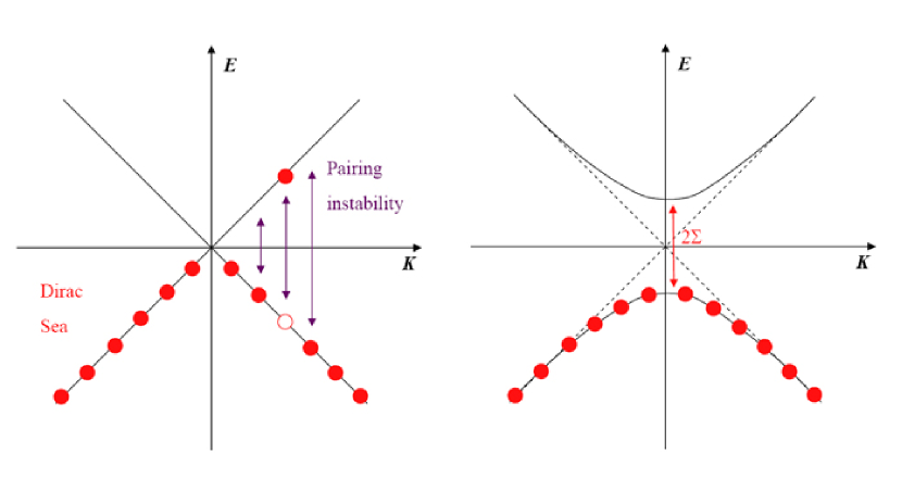
Figure 7.1: $\bar{\psi}\psi$ pairing instability leading to a chirally broken phase of the vacuum.

In this energy-momentum diagram it can be seen that, due to the pairing of the quark anti-quark pairs, an energy gap of $2\Sigma$ is created between the highest (quark) and lowest (anti-quark) states. This gap then represents a rest mass that is far greater than the current mass i.e. $\Sigma\gg m$, which can be interpreted as a physical representation of a vacuum with broken chiral symmetry.

In Sec. 7.3 we will go onto discuss how a variation in thermodynamic conditions could lead to the restoration of chiral symmetry, and how extreme variation then leads to exotic strongly interacting matter i.e. colour superconductivity/superfluidity.

7.3 The QCD Phase Diagram

When it had become clear that hadrons were indeed a state of confined quarks and gluons, it was suggested that they should become deconfined at high temperatures or densities when the hadrons strongly overlap and lose their individuality[11]. In this picture, we then have two phases, the "hadronic phase" where quarks and gluons are confined, and the quark-gluon plasma where they are deconfined. Such phases of strongly interacting matter and the associated transitions between them, with external thermodynamic control parameters like temperature and density, make up a map of The QCD Phase Diagram.

7.3.1 A Classic Phase Diagram of $H_{2}O$

A classical example of a phase diagram is that of $H_{2}O$, Fig. 7.2.

Figure 7.2: The phase diagram of $H_{2}O$ (not to scale).

In this diagram the thermodynamic control parameters are temperature $T$ and pressure $P$, and the different manifestations (or phases) of $H_{2}O$ are separated into three regions of ice, water and steam, with the separating boundaries between them marked by the equilibrium coexistence curves $P(T)$. Thus, a first order phase transition such as melting or boiling is observed when moving along a path in the $(T,P)$ plane that crosses the equilibrium boundaries. In this diagram there are two special points: the critical point ($T_{c}=650K$, $P_{c}=2.21\times 10^{7}Nm^{-2}$) where the phases of water and vapour become indistinguishable, and the triple point ($T_{tr}=273.16K$,$P_{tr}=600Nm^{-2}$) where all three phases coexist.

7.3.2 A Map of the QCD Phase Diagram

A possible schematic of the QCD phase diagram is presented in Fig. 7.3, with the thermodynamic control parameters temperature, $T$, and baryon chemical potential, $\mu$.

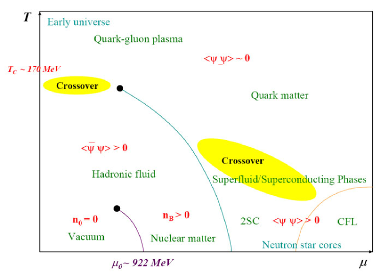
Figure 7.3: The proposed phase diagram of QCD (not to scale).

In this diagram we can note several locations which have analogues in condensed matter physics. The first location is the bottom left hand corner of the phase diagram where $T$ and $\mu$ are both small. Here the thermodynamic behavior of QCD can be described as that of a vapour of hadrons, i.e. composite states of quarks and/or anti-quarks. In this location extensive work has been carried out to classify and quantify the bound states of strongly interacting matter, hence, this area has a certain amount of resemblance to relativistic atomic physics. It is then argued, and has been shown through numerical calculations that as we increase $T$ the hadronic vapour phase cannot persist. Eventually there comes a point, found to be $T_{c}\simeq 170MeV$[25], where the dominant degrees of freedom are no longer hadrons, but quarks and gluons themselves. This "gas" of strongly interacting matter is known as the quark-gluon plasma (QGP), thus the upper left region of the phase diagram has the classic analogue of relativistic plasma physics. Two possible candidates for the formation of the QGP phase are the early universe, immediately after the Big Bang, and high energy collisions between nuclear particles.

The final area of the phase diagram, and also the most elusive, lies along the $\mu$-axis. Unlike simulations along the $T$-axis, lattice gauge theory simulation become ineffective when applied to QCD with $\mu\neq 0$. However, through extrapolation methods it is seen that as you increase $\mu$, for zero temperature, the ground state (i.e. the vacuum) persists until $\mu$ reaches the value of nuclear matter (nucleon rest mass minus the binding energy), at which point it becomes energetically favorable to fill the ground state with a bound nucleonic fluid. This onset value is estimated at $\mu_{0}=922MeV$, at which point baryon density $n_{B}$ jumps from zero to nuclear density $n_{B0}\simeq 0.16fm^{-3}$. This is referred to in [13] as ’room chemical potential’ as the vacuum and nuclear matter coexist at this point. Extrapolation methods, can be employed for densities up to $2-3n_{B0}$, however beyond this we are forced to rely on approximate treatments such as the MIT bag model or the NJL model. Through such treatments it is estimated that as $n_{B}$ increases we again expect a transition from a phase where matter exists in the form of nucleons to one where the dominant degrees of freedom are quarks and gluons. This phase of dense, strongly interacting, matter is believed to exist at the cores of neutron stars. It is also speculated that under such conditions a phenomenon similar to the Bardeen-Cooper-Schrieffer (BCS) instability, that leads to superconductivity in metals and superfluidity in liquid ³He at low temperature, results in the formation of diquark pairs and the onset of a colour superconducting/superfluid phase (see Sec. 7.4). Therefore, the lower right region of the diagram has similarities to a branch of condensed matter physics; and it is this region of the phase diagram with which this thesis will be dealing.

7.3.3 Restoration of Chiral Symmetry

Before we go on to coloured BCS phenomenon (the area with which this thesis is concerned) we will discuss the restoration of chiral symmetry in the various areas of the phase diagram, in particular the areas of high $T$ and $\mu$, i.e. the upper part around to the bottom right of the phase diagram.

$<\bar{\psi}\psi>\sim 0$ For Extreme $T$

It has been seen through numerical simulations that the onset of QGP coincides with the restoration of chiral symmetry[25]. As you move from the phase of bound strongly interacting matter, at low temperature and density, up to the high temperature region dominated by QGP there is seen to be a drop in the vacuum quark condensate i.e. the order parameter $<\bar{\psi}\psi>$ tends to zero in the QGP phase. However, to be precise it has been shown [13] that the order parameter $<\bar{\psi}\psi>$ doesn’t strictly vanish, but rather drops very steeply in the transition region, and this transition is seen to occur at $T_{c}\simeq 170MeV$. Thus, in the QCD phase diagram the formation of QGP along the $\mu=0$ axis is naturally referred to as a crossover rather than a true first or second order phase transition. In a hand waving way we can interpret the "destruction" of the vacuum quark condensate as a result of the high temperature influence on the strong coupling constant, $g(T)$. We can say that at very high temperatures, where QGP occurs, large energies are exchanged in inter-particle collisions, which results in the weakening of the strong interaction due to asymptotic freedom. Therefore, as the energy needed to excite quark anti-quark pairs is no longer below the binding energy between them the quark condensate does not form, which in turn leads to the restoration of chiral symmetry.

$<\bar{\psi}\psi>\sim 0$ For Extreme $\mu$

As previously discussed, to study the high density region of the QCD phase diagram, i.e. above $2-3n_{B0}$ (and $T\approx 0$), one must employ alternative models to lattice gauge theory such as the MIT bag model and the NJL model. Each model has its pros and cons: the most important characteristic of the bag model is its property of quark confinement, and that of the NJL model is chiral symmetry and its spontaneous breakdown in the vacuum; on the other hand the bag model violates chiral symmetry and the NJL model does not possess confinement. So one must decide which property is of greater importance and employ the appropriate model. Through simulations, using the NJL model, it is seen that as you increase baryon density beyond the nuclear density $n_{B0}$, i.e. move from the hadronic phase to that of strongly interacting matter, a phase transition takes place from the chirally broken phase to one of restored chiral symmetry [12]. This restoration of chiral symmetry in the high density regime can be considered due to the quarks becoming the dominant degrees of freedom at this density. At extreme densities ($\mu\sim 1200MeV$ [13]) hadrons strongly overlap, lose their individuality and start to behave like one big mass of quark matter; which is thought to occur in neutron stars. Being fermions, the quarks occupy the Fermi sea up to the level $E_{F}$. This leads to $\bar{\psi}\psi$ vacuum excitations, for $|k|\ll k_{F}$, becoming Pauli-blocked. Therefore, at some point, these pairs require so much energy to excite that it becomes preferable to revert to a chirally symmetric ground state. In this way, at high density, chiral symmetry is restored.

7.4 Coloured BCS Phenomenon

7.4.1 BCS Processes

In BCS theory the pairing of Fermions (known as Cooper pairs) leads to the formation of Bosonic particles, which condense and leave an energy gap $2\Delta$ that is equal to the energy of the binding between the pair, Fig. 7.4. In metals this BCS condensation of electrons leads to superconductivity, i.e. the flow of electric current without resistance. It is also seen that BCS condensation is accompanied by the breaking of the $U(1)$ local electromagnetic gauge symmetry. Such BCS processes are also relevant in the study of superfluidity (the flow of fluid with negligible viscosity). One type of superfluid, ${}^{4}He$, is a Bosonic fluid, and simply undergoes Bose-Einstein condensation at low temperatures. However, ${}^{3}He$, a Fermionic fluid, undergoes a BCS type process which leads to the condensation of bound Cooper pairs. As both superconductor and superfluid have an energy gap, the way to distinguish between the two is that a superfluid is characterised by a ground state which does not respect a global symmetry of the underlying action.

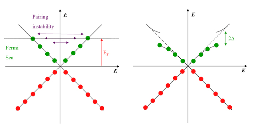
Figure 7.4: $\psi\psi$ pairing instability leading to super-conductivity.

7.4.2 BCS in QCD

Due to the strong attraction between quarks the BCS process leads to some interesting results in QCD. One of these, as we have already seen in sec. 7.2.3, is the condensation of quark-antiquark pairs. This leads to spontaneous Chiral symmetry breaking, and a resulting effective quark mass which is much higher than the current mass. Also, it is believed that at high densities, when chiral symmetry is restored, and quarks are deconfined, condensation of diquark pairs occurs; and the resulting $qq$ wave function is a gauge non-singlet. This condensation leads to the formation of an energy gap separating the ground and excited states by $2\Delta$. As in "orthodox" BCS processes, this condensation of diquark pairs is accompanied by the breaking of local colour gauge symmetry, $SU(3)_{c}$; and in analogy with electromagnetic superconductivity this high density phenomenon is known as colour superconductivity (CSC).

If we were able to conduct Lattice QCD simulations at $\mu\neq 0$ it could be possible that we’d see the colour superconducting phase. However, due to the sampling weight, used in Monte-Carlo methods, becoming complex, to study quark matter in the high density phase we require effective field theories, such as the NJL model. The NJL model is a purely Fermionic model, containing no gauge degrees of freedom, and interactions are simply represented by a four-point interaction. One of the most important features that makes the NJL model an ideal effective theory of QCD at high density is that it not only observes the same (Chiral) symmetries of QCD, but the breaking of these symmetries in the vacuum is analogous to BCS superconductivity. For this reason it is viewed as an appropriate model to study coloured BCS phenomena. However, in the NJL model the $qq$ wave function is gauge singlet, which implies the ground state is not superconducting, but rather superfluid.

Chapter 8 The Nambu-Jona-Lasino Model

Quantum chromodynamics is the accepted theory of strong interactions and at short distances is highly successful. However, as discussed in the previous chapter, for larger distances where perturbative techniques break down lattice gauge theory is required to calculate the QCD expectation values. This method itself has problems such as the requirement of huge computing power, problems associated with including fermions on a discretized lattice, problems for $\mu\neq 0$, etc (See Sec. 7.1.2). For this reason it is reasonable to isolate the relevant physics associated with a process of interest and construct an approximate model of the exact theory that accentuates the main features of the theory; to study strongly interacting matter at high density (i.e. $\mu\neq 0$) we do just this. In this chapter we start off by discussing the Nambu-Jona-Lasino (NJL) model as a model of QCD, its chiral symmetry and other associated technical issues, and also the benefits of its use for lattice calculations at high density. We then go onto discuss the lattice transcription of the NJL model in $2+1$ dimensions. Finally we discuss QCD calculations involving the lattice NJL model in 2+1 dimensions, referring to the results of [12] and how they relate to the investigations of this thesis.

8.1 The NJL Model of QCD

Non-perturbative QCD calculations in the high density regime are next to impossible due to the measure of the Euclidean path integral becoming complex for baryon chemical potential $\mu\neq 0$. This phenomenon, known as the sign problem, involves the QCD path integral effectively generating meaningless complex probabilities. One way to overcome this problem is by the use of the pre-QCD model of Nambu and Jona-Lasino [23, 24]. In this model nucleons were considered to interact through a two body interaction, and the resulting lagrangian was symmetric under the full chiral symmetry group given in Eqn. (LABEL:full_chiral_symmetry_group). However, in accordance with experimental observation the $U(1)_{A}$ symmetry was later excluded.

As this theory was conceived before the advent of quarks, Nambu and Jona-Lasino used nucleons as the elementary building blocks of the model. In analogy to the effective electron-electron interaction in BCS theory the nucleon-antinucleon attractive interaction was considered to be responsible for the formation of Cooper pairs of nucleons and antinucleons, which results in a nucleon condensate. This condensate would then lead to a vacuum mass gap and the breaking of chiral symmetry, where the pion could then be identified as the Goldstone boson occurring in the theory due to the breaking of the axial symmetry.

With the possibility of quarks the NJL model can be reinterpreted as a simple model of QCD, with the quarks taking the place of the nucleons. However in this simplified model the strong interaction, mediated by the gluons, is excluded; instead the interaction between quarks is assumed to be a point-like four-point interaction (for $N_{f}=2$). This means it does not describe quark confinement - the phenomenon whereby single isolated quarks are never observed. On the other hand the NJL model has other interesting properties which make it a suitable substitute for QCD, i.e. the model’s global symmetries and the patterns of their breaking are similar to those of QCD [22].

8.1.1 NJL Lagrangian

In Euclidean space, the original lagrangian density describing the NJL model with $N_{f}=2$ quark flavours in the isospin representation of $SU(2)$ can be written as

$$\mathcal{L}=\overline{\psi}^{p}(\partial/\hskip 1.00006pt+m_{0})\tau^{pq}_{0}\psi^{q}-\frac{g^{2}}{2}[(\overline{\psi}^{p}\tau^{pq}_{0}\psi^{q})^{2}-(\overline{\psi}^{p}\gamma_{5}\vec{\tau}^{pq}\psi^{q})^{2}]$$ (8.1)

where $\psi$ and $\overline{\psi}$ are independent Grassmann Dirac 4-spinors representing the quark fields, $m_{0}$ is the current, or bare-mass of the quark, $\vec{\tau}\equiv(\tau_{1},\tau_{2},\tau_{3})$ is a vector of the $2\times 2$ Pauli matrices, which run over internal isospin or flavour degrees of freedom, and $\tau_{0}$ is the unit matrix.

When the NJL model was reinterpreted as a quark model, with $\psi$ as the quark field with two flavour and 3 colour degrees of freedom, it was kept in the original NJL form (8.1), and in this thesis we will work with this form of the model. However, Eqn. (8.1) is not unique and other chirally symmetric interaction terms can be included. A more general form of the NJL model is given as [11]:

$$\mathcal{L}=\overline{\psi}^{p}(\partial/\hskip 1.00006pt+m_{0})\tau^{pq}_{0}\psi^{q}-\frac{g^{2}}{2}[(\overline{\psi}^{p}\tau^{pq}_{0}\psi^{q})^{2}-(\overline{\psi}^{p}\vec{\tau}^{pq}\psi^{q})^{2}+(\overline{\psi}^{p}\gamma_{5}\tau^{pq}_{0}\psi^{q})^{2}-(\overline{\psi}^{p}\gamma_{5}\vec{\tau}^{pq}\psi^{q})^{2}]$$ (8.2)

8.1.2 Bosonization

Through the introduction of auxiliary scalar and pseudo-scalar fields, $\sigma$ and $\vec{\pi}$, the NJL model can be rewritten in a bosonized form, which makes it easier to treat both numerically and analytically. Starting with the NJL Lagrangian (8.1) we can introduce the generating functional

$$Z\sim\int\mathcal{D}\psi\mathcal{D}\bar{\psi}\exp[\int d^{4}x\mathcal{L}(\psi,\bar{\psi})]$$ (8.3)

Then using the fact that path integrals of Gaussian functions can be performed exactly [22],

$$\int\mathcal{D}\Phi\exp[\int d^{4}x(\pm A\Phi-B\Phi^{2})]\sim\exp[\int d^{4}x\frac{A^{2}}{4B}]$$ (8.4)

we can write:

$$\exp[\int d^{4}xG(\bar{\psi}\psi)^{2}] \sim \int\mathcal{D}\sigma\exp\{\int d^{4}x[(\bar{\psi}\psi)\sigma-\frac{1}{4G}\sigma^{2}]\}$$

$$\exp[\int d^{4}xG(\bar{\psi}i\gamma_{5}\vec{\tau}\psi)^{2}] \sim \int\mathcal{D}\pi\exp\{\int d^{4}x[(\bar{\psi}i\gamma_{5}\vec{\tau}\cdot\vec{\pi}\psi)-\frac{1}{4G}\vec{\pi}^{2}]\}$$

where we have $G=-\frac{g^{2}}{2}$. Therefore, we can rewrite (8.3) in a bosonized form as

$$Z \sim \int\mathcal{D}\psi\mathcal{D}\bar{\psi}\mathcal{D}\sigma\mathcal{D}\vec{\pi}\exp\{\int d^{4}x[\bar{\psi}[\partial/\hskip 1.00006pt+m_{0}+(\sigma+i\gamma_{5}\vec{\tau}\cdot\vec{\pi})]\psi$$ (8.6)

$$- \frac{1}{4G}(\sigma^{2}+\vec{\pi}\cdot\vec{\pi})]\}$$

Now using $\Phi=\sigma+i\vec{\pi}\cdot\vec{\tau}$ and $\sigma^{2}+\vec{\pi}\cdot\vec{\pi}=\frac{1}{2}Tr\Phi^{\dagger}\Phi$ we have the bosonized form of the NJL lagrangian:

$$\mathcal{L}=\bar{\psi}[\partial/\hskip 1.00006pt+m_{0}+(\sigma+i\gamma_{5}\vec{\tau}\cdot\vec{\pi})]\psi-\frac{1}{8G}Tr\Phi^{\dagger}\Phi$$ (8.7)

8.1.3 Chiral Symmetry of the NJL Model

The simplest way to show that the NJL lagrangian is symmetric under chiral transformations (7.9) is to use the bosonized lagrangian in (8.7). For vanishing mass the kinetic term can be easily shown to be symmetric:

$$\bar{\psi}\gamma^{\mu}\partial_{\mu}\psi\rightarrow\bar{\psi}\bar{V}\gamma^{\mu}\partial_{\mu}V\psi = \bar{\psi}\gamma^{\mu}(V^{\dagger}_{L}V_{L}P_{L}+V^{\dagger}_{R}V_{R}P_{R})\partial_{\mu}\psi$$ (8.8)

$$= \bar{\psi}\gamma^{\mu}(P_{L}+P_{R})\partial_{\mu}\psi$$

$$= \bar{\psi}\gamma^{\mu}\partial_{\mu}\psi$$

However, the symmetry of the bosonic terms is a little more subtle. Bosonic fields, as in the last term of (8.7), transform as[19]:

$$\Phi\rightarrow V_{L}\Phi V^{\dagger}_{R}$$ (8.9)

Using this we can show that the first bosonic term is symmetric, by first writing it in the form:

$$\bar{\psi}(\sigma+i\gamma_{5}\vec{\tau}\cdot\vec{\pi})\psi = \bar{\psi}_{L}(\sigma+i\vec{\tau}\cdot\vec{\pi})\psi_{R}+\bar{\psi}_{R}(\sigma-i\vec{\tau}\cdot\vec{\pi})\psi_{L}$$ (8.10)

$$= \bar{\psi}_{L}\Phi\psi_{R}+\bar{\psi}_{R}\Phi^{\dagger}\psi_{L}$$

where

$$\Phi=\left(\begin{array}[]{cc}\sigma+i\pi_{3}&\pi_{2}+i\pi_{1}\\ -\pi_{2}+i\pi_{1}&\sigma-i\pi_{3}\\ \end{array}\right)$$ (8.11)

Now under the chiral transformation we have:

$$\bar{\psi}_{L}V^{\dagger}_{L}\Phi V_{R}\psi_{R}+\bar{\psi}_{R}V^{\dagger}_{R}\Phi^{\dagger}V_{L}\psi_{L}$$ (8.12)

which is symmetric, as the bosonic field $\Phi$ transforms as (8.9).

8.2 The Lattice Transcription of the NJL Model

In this thesis we use the lattice transcription of the NJL model in $2+1$ dimensions, as used in [12]. We replace the space-time continuum with a 3-dimensional lattice, where each site is separated from its nearest neighbours by an arbitrary lattice spacing $a$. In dimensions $d>2+1$ this lattice spacing must be chosen for the effect of introducing an ultra-violet (UV) cutoff $\Lambda\sim a^{-1}$, which then regularises the divergences and makes the theory mathematically well-defined, however, in $d=2+1$ dimensions the theory is renormalizable and well defined on the lattice for an arbitrary cutoff[14].

The structure of our model consists of the fermion fields being defined on the lattice sites $x$ and the bosonic fields being defined on the dual lattice sites $\tilde{x}$, translated from the original lattice by $(\frac{1}{2},\frac{1}{2},\frac{1}{2})$. The space-time integrals and differentials are represented by sums and finite differences, so that in the staggered fermion notation the noninteracting quark action

$$S=\int d^{3}x\bar{\psi}(\partial/\hskip 1.00006pt+m_{0})\psi$$ (8.13)

is given by

$$S=\sum_{x}a^{3}\{{\frac{1}{2a}\sum^{2}_{\nu=0}\eta_{\nu}(x)[(\bar{\chi}_{x}\chi_{x+\hat{\nu}})-(\bar{\chi}_{x}\chi_{x-\hat{\nu}})]+m_{0}(\bar{\chi}_{x}\chi_{x})}\}$$ (8.14)

where $\bar{\chi}$ and $\chi$ are the Grassmann-valued staggered fermion fields defined on the lattice sites, and $\eta_{\nu}(x)$ is the Kawamoto-Smit phase $(-1)^{x_{0}+...x_{\nu-1}}$. Now, using this definition of the free action, we can go onto describe the construction of the full NJL model as used in this thesis.

Lattice NJL Model for $\mu=0$

The NJL model on the lattice for $\mu=0$, in its bosonised form, is defined by the Euclidean action

$$S=\sum_{x}\bar{\chi}M[\Phi]\chi+\frac{1}{g^{2}}\sum_{\tilde{x}}tr\Phi^{{\dagger}}\Phi\\$$

where $\chi$, $\overline{\chi}$ are, as before, the fermionic fields defined on the lattice sites, and $\Phi\equiv\sigma+i\overrightarrow{\pi}\cdot\overrightarrow{\tau}$ is a $2\times 2$ matrix of bosonic auxiliary fields, again as before, defined on the dual lattice sites. Also, $M[\Phi]$ is the kinetic operator, and is in the form for staggered lattice fermions interacting with scalar fields,

$$M^{pq}_{xy} = \frac{1}{2}\delta^{pq}\sum_{\nu=0}^{2}[\eta_{\nu}(x)(\delta_{yx+\hat{\nu}}-\delta_{yx-\hat{\nu}})+2m\delta_{xy}]$$ (8.15)

$$+ \frac{1}{8}\delta_{xy}\sum_{<\tilde{x},x>}[\sigma(\tilde{x})\delta^{pq}+i\varepsilon(x)\vec{\pi}(\tilde{x})\cdot\vec{\tau}^{pq}]$$

Here the parameters are bare fermion mass $m$ and coupling constant $g^{2}$. The Pauli matrices, $\vec{\tau}$, are normalized to $\textrm{tr}(\tau_{i}\tau_{j})=2\delta_{ij}$ and act on the internal $SU(2)$ isospin indices $p,q=1,2$, and $\varepsilon(x)$ denotes the phase $(-1)^{x_{0}+x_{1}+x_{2}}$. Finally we have $<\widetilde{x},x>$, which represents the sum over the set of $8$ dual lattice sites neighbouring $x$. In this bosonized form we can integrate over the auxiliary $\Phi$ fields which leads to an equivalent action in terms of fermions that self-interact via a four-point contact term proportional to $g^{2}$, as shown in Sec. 8.1.2.

Lattice NJL Model for $\mu\neq 0$

To introduce a chemical potential $\mu$ into a fermionic field theory we must incorporate a term of the form $\mathcal{L}_{\mu}=\mu\bar{\psi}\gamma_{0}\psi$ into the fermionic Lagrangian. The inclusion of this term can be understood in a simple way by considering that to introduce a source into a Lagrangian we must incorporate a source term of the type $\mathcal{L}_{source}=J\phi$, where $J$ is the source for the field $\psi$. Therefore, as $\bar{\psi}\gamma_{0}\psi\sim\psi^{\dagger}\psi$ is the quark number operator $N_{q}$, we can think of $\mu$ as a source for this operator, which leads to the creation of fermions over anti-fermions as a more energetically favourable process. Therefore, the chemical potential term would then be incorporated into the partition function in the usual way, as $e^{-\mu N_{q}}$. However, introducing a chemical potential in a discretized field theory is not as simple. We cannot simply implement a term of the form given above and naively discretise it, as it can be shown that this leads to divergences in the energy density of the theory [25, 26]. This can be resolved if we consider that incorporating a chemical potential in the form given above is like the zeroth component of a vector potential interaction term in a fermionic Lagrangian, $\bar{\psi}\gamma_{\mu}\psi A^{\mu}\Rightarrow\bar{\psi}\gamma_{0}\psi A^{0}$. Thus, due to this similarity to a gauge field, we must incorporate the chemical potential term in a "gauge-invariant" way. This is done by introducing $\mu$ into the zeroth derivative by multiplying the forward time difference by $e^{\mu}$ and the backward time difference by $e^{-\mu}$. In this way the kinetic operator (8.15) becomes

$$M^{pq}_{xy} = \frac{1}{2}\delta^{pq}[(e^{\mu}\delta_{yx+\hat{0}}-e^{-\mu}\delta_{yx-\hat{0}})$$ (8.16)

$$+ \sum_{\nu=1,2}\eta_{\nu}(x)(\delta_{yx+\hat{\nu}}-\delta_{yx-\hat{\nu}})+2m\delta_{xy}]$$

$$+ \frac{1}{8}\delta_{xy}\sum_{<\tilde{x},x>}[\sigma(\tilde{x})\delta^{pq}+i\varepsilon(x)\vec{\pi}(\tilde{x})\cdot\vec{\tau}^{pq}]$$

Introduction of the Diquark Sources

Due to limitations of computer memory we are forced to work on a finite volume system, and working under such conditions leads to certain complications. One such issue is that due to finite volume effects on spontaneous symmetry breaking. A simple example of this phenomenon is seen in the O(N) model. One of the most important properties of this model is the effect of spontaneous spin symmetry breaking at the critical temperature, Appendix B. In the 2-dimensional O(N) model, above the critical temperature, the spins at each lattice site are randomly orientated due to thermal fluctuations, hence we have the average value $<S_{i}>=0$. When we hit the critical temperature, thermal fluctuations become less dominant compared to spin interactions and the correlation length increases, this in turn leads to spontaneous magnetisation (i.e. magnetisation with a zero external field). Then, at $T=0$ the magnetisation is at its maximum, and the correlation length is comparable to the size of the lattice. However, it is seen that such effects only occur in the thermodynamic limit

$$M=\lim_{N\rightarrow\infty}\frac{1}{N}\sum_{i}<S_{i}>\neq 0$$ (8.17)

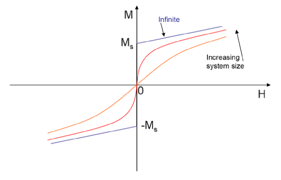
Figure 8.1: Magnetisation $M$ against external field $H$.

These finite volume effects are shown in Fig. 8.1, which shows magnetisation verses external magnetic field. It can be seen that spontaneous symmetry breaking only occurs in the limit of $N\rightarrow\infty$. So how can we simulate an infinite lattice? This problem can be overcome in computational calculations by including a symmetry breaking term that represents the external field. Therefore, for a finite volume system we can conduct simulations with various values of the external field, such as the magnetic field $H$ in the O(N) model, and then extrapolate to the limit of the field going to zero, $H\rightarrow 0$. This then gives the spontaneous magnetisation value of the system at temperature $T$. A similar problem is seen in the study of chiral symmetry breaking, where we include a finite bare mass $m$ to allow the measurement of the chiral condensate $<\bar{\psi}\psi>$ on a finite volume. It is for a similar reason we include the diquark and anti-diquark symmetry breaking terms, which allows us to measure the values for $<\psi\psi>$ and $<\bar{\psi}\bar{\psi}>$ condensates. The implementation of such diquark symmetry breaking terms requires the introduction of diquark and anti-diquark fields $j$ and $\bar{j}$ that can be taken to zero for the infinite volume system. Therefore, in analogy with the mass term (for the measurement of the chiral condensate), and the external field term (in the O(N) model for the measurement of spontaneous magnetisation) we include the following terms into the NJL Lagrangian:

$$j\chi^{tr}\tau_{2}\chi+\bar{j}\bar{\chi}\tau_{2}\bar{\chi}^{tr}$$ (8.18)

Final Form of the Model and its Symmetries

We can now write down the full NJL model, as studied in this thesis:

$$S_{NJL}=S_{fer}+S_{bos}$$ (8.19)

where the fermionic and bosonic parts of the action are:

$$S_{fer}=\sum_{x}\bar{\chi}M[\Phi]\chi+j\chi^{tr}\tau_{2}\chi+\bar{j}\bar{\chi}\tau_{2}\bar{\chi^{tr}}$$ (8.20)

$$S_{bos}=\frac{1}{g^{2}}\sum_{\tilde{x}}tr\Phi^{{\dagger}}\Phi$$ (8.21)

where $M[\Phi]$ is given in Eqn. (8.16). To construct the partition function of this system we rewrite the fermion part of the action by defining a bispinor $\Psi^{tr}=(\bar{\chi}^{tr},\chi)$. In this, Gor’kov, basis we can write the fermion action as

$$S_{fer}=\Psi^{tr}\mathcal{A}\Psi$$ (8.22)

where the Nambu-Gor’kov matrix $\mathcal{A}$ is

$$\mathcal{A}^{pq}_{xy}=\left(\begin{array}[]{cc}\bar{j}\tau_{2}^{pq}\delta_{xy}&\frac{1}{2}M^{pq}_{xy}\\ -\frac{1}{2}M^{qp}_{yx}&j\tau_{2}^{pq}\delta_{xy}\\ \end{array}\right)$$ (8.23)

In this basis we can integrate out the fermion fields, which leaves us with the following Euclidean path integral:

$$Z=\int D\Phi^{\dagger}D\Phi\sqrt{\det 2\mathcal{A}}\exp(-S_{bos}(\Phi))$$ (8.24)

The discretized NJL model, given by Eqns. (8.19)-(8.21) and (8.16), still has the full QCD symmetry $SU(2)_{L}\times SU(2)_{R}\times U(1)_{B}$, as discussed in sec. 8.1.3. But now the projection operators (7.6) become $P_{R/L}\rightarrow P_{e/o}=\frac{1}{2}[1\pm\varepsilon(x)]$, which project onto even and odd sublattices, respectively; and the transformations take the form:

$$\chi \rightarrow(V_{e}P_{e}+V_{o}P_{o})\chi\qquad\bar{\chi}\rightarrow\bar{\chi}(P_{e}V_{e}^{\dagger}+P_{o}V_{o}^{\dagger})$$ (8.25)

$$\Phi \rightarrow V_{o}\Phi V_{e}^{\dagger}\qquad[V_{e},V_{o}\in SU(2)]$$

$$\chi \rightarrow e^{i\alpha}\qquad\bar{\chi}\rightarrow\bar{\chi}e^{-i\alpha}\qquad[e^{i\alpha}\in U(1)_{B}]$$ (8.26)

The symmetry of the diquark source terms, Eqn. (8.18), requires an extra explanation. These terms were added to break baryon symmetry, $U(1)_{B}$, hence allowing the measurement of the diquark condensate as $j\rightarrow 0$. Therefore, under the transformation (8.26) it is not symmetric,

$$j\chi^{tr}\tau_{2}\chi+\bar{j}\bar{\chi}\tau_{2}\bar{\chi}^{tr}\rightarrow j\chi^{tr}\tau_{2}\chi e^{i2\alpha}+\bar{j}\bar{\chi}\tau_{2}\bar{\chi}^{tr}e^{-i2\alpha},$$ (8.27)

where the symmetry is restored for vanishing $j$ and $\bar{j}$. Under the $SU(2)$ symmetry, (8.25), the terms are still symmetric. We can show this by considering only the $j$ term:

$$j\chi^{tr}\tau_{2}\chi \rightarrow j\chi^{tr}(V_{e}^{tr}P_{e}+V_{o}^{tr}P_{o})\tau_{2}(V_{e}P_{e}+V_{o}P_{o})\chi$$

$$= j\chi^{tr}(V_{e}^{tr}\tau_{2}V_{e}P_{e}+V_{o}^{tr}\tau_{2}V_{o}P_{o})\chi$$

Now using the identity: $\tau_{2}U\tau_{2}=U^{*}$ we can write:

$$j\chi^{tr}(\tau_{2}V_{e}^{\dagger}V_{e}P_{e}+\tau_{2}V_{o}^{\dagger}V_{o}P_{o})\chi = j\chi^{tr}\tau_{2}(P_{e}+P_{o})\chi$$ (8.29)

$$= j\chi^{tr}\tau_{2}\chi$$

which shows the symmetry of the diquark source term (similarly for the anti-diquark source term).

8.3 QCD Dynamics using the NJL Model

Previous studies of the $2+1$d NJL model have shown that a strong first order phase transition, at $\mu_{c}\simeq\Sigma\simeq 0.65$, takes place to a chirally symmetric state [12]. This transition is seen to be accompanied by the onset of a non-vanishing density of baryon charge in the ground state. However, in this high density region it is also seen, for $2+1$ dimensions, that there is no diquark condensation and the $U(1)_{B}$ symmetry is not broken, and there’s no evidence of a non-zero energy gap. More interestingly, it is seen that the diquark condensate scales non-analytically at high density, $<\psi\psi>\propto j^{\frac{1}{\delta}}$.

In this section we will look at how these results were determined, and more importantly (for our work) how the non-analytic behaviour of the diquark condensate could imply superfluidity.

8.3.1 Phase Transitions at High Density

Chiral Condensate

Chiral symmetry restoration is signalled by the first order transition of the chiral condensate, $<\bar{\psi}\psi>\rightarrow 0$, which is determined as:

$$<\bar{\psi}\psi> = \frac{1}{V}\frac{\partial\ln Z}{\partial m}=\frac{1}{ZV}\frac{\partial Z}{\partial m}$$

$$= \frac{1}{ZV}\frac{\partial}{\partial m}\int\mathcal{D}\Phi^{\dagger}\mathcal{D}\Phi\sqrt{\det 2\mathcal{A}}\exp(-S_{bos}(\Phi))$$

$$= \frac{1}{ZV}\int\mathcal{D}\Phi^{\dagger}\mathcal{D}\Phi\frac{1}{2}\frac{1}{\sqrt{\det 2\mathcal{A}}}\frac{\partial(\det 2\mathcal{A})}{\partial m}\exp(-S_{bos}(\Phi))$$

using $\det 2\mathcal{A}=\exp(\textrm{tr}\ln(2\mathcal{A}))$, we have:

$$<\bar{\psi}\psi> = \frac{1}{ZV}\int\mathcal{D}\Phi^{\dagger}\mathcal{D}\Phi\frac{1}{2}\textrm{tr}(\frac{2\frac{\partial\mathcal{A}}{\partial m}}{2\mathcal{A}})\frac{\det 2\mathcal{A}}{\sqrt{\det 2\mathcal{A}}}\exp(-S_{bos}(\Phi))$$

$$= \frac{1}{ZV}\int\mathcal{D}\Phi^{\dagger}\mathcal{D}\Phi\frac{1}{2}\textrm{tr}(\mathcal{A}^{-1}\frac{\partial\mathcal{A}}{\partial m})\sqrt{\det 2\mathcal{A}}\exp(-S_{bos}(\Phi))$$

From (8.16) and (8.23) we have

$$\frac{\partial\mathcal{A}}{\partial m}=\left(\begin{array}[]{cc}0&\frac{1}{2}\delta\\ -\frac{1}{2}\delta&0\\ \end{array}\right)$$ (8.32)

therefore (LABEL:qbarq) becomes

$$<\bar{\psi}\psi>=\frac{1}{Z}\int\mathcal{D}\Phi^{\dagger}\mathcal{D}\Phi\frac{1}{4V}\textrm{tr}(\mathcal{A}^{-1}\left(\begin{array}[]{cc}0&\frac{1}{2}\delta\\ -\frac{1}{2}\delta&0\\ \end{array}\right))\sqrt{\det 2\mathcal{A}}\exp(-S_{bos}(\Phi))$$ (8.33)

Then, the expectation we calculate is:

$$<\bar{\psi}\psi>=<\frac{1}{4V}\textrm{tr}(\mathcal{A}^{-1}\left(\begin{array}[]{cc}0&\frac{1}{2}\delta\\ -\frac{1}{2}\delta&0\\ \end{array}\right))>$$ (8.34)

Baryon Charge Density

As chiral symmetry is restored at high density, and nucleons dissociate into quarks, there is seen to be an onset of a non-vanishing density of baryon charge in the ground state, $n_{B}=<\bar{\psi}\gamma_{0}\psi>$, which is determined using Eqn. (8.24),

$$n_{B} = <\bar{\psi}\gamma_{0}\psi>=\frac{1}{V}\frac{\partial\ln Z}{\partial\mu}=\frac{1}{ZV}\frac{\partial Z}{\partial\mu}$$

$$= \frac{1}{ZV}\int\mathcal{D}\Phi^{\dagger}\mathcal{D}\Phi\frac{1}{2}\textrm{tr}(\mathcal{A}^{-1}\frac{\partial\mathcal{A}}{\partial\mu})\sqrt{\det 2\mathcal{A}}\exp(-S_{bos}(\Phi))$$

where, as before, we find using (8.16) and (8.23)

$$\frac{\partial\mathcal{A}}{\partial\mu}=\left(\begin{array}[]{cc}0&\frac{1}{2}\frac{\partial M}{\partial\mu}\\ -\frac{1}{2}\frac{\partial M^{tr}}{\partial\mu}&0\\ \end{array}\right)$$ (8.36)

where

$$\frac{\partial M}{\partial\mu} = \frac{1}{2}\delta^{pq}[\exp(\mu)\delta_{y,x+\hat{0}}+\exp(-\mu)\delta_{y,x-\hat{0}}]$$

$$\frac{\partial M^{tr}}{\partial\mu} = \frac{1}{2}\delta^{pq}[\exp(\mu)\delta_{x+\hat{0},y}+\exp(-\mu)\delta_{x-\hat{0},y}]$$

$$= \frac{1}{2}\delta^{pq}[\exp(\mu)\delta_{y,x-\hat{0}}+\exp(-\mu)\delta_{y,x+\hat{0}}]$$

Now, defining:

$$\mathcal{X} = \frac{\partial\mathcal{A}}{\partial\mu}$$ (8.40)

$$= \frac{1}{4}\left(\begin{array}[]{cc}0&\delta^{pq}[e^{\mu}\delta_{y,x+\hat{0}}+e^{-\mu}\delta_{y,x-\hat{0}}]\\ -\delta^{pq}[e^{\mu}\delta_{y,x-\hat{0}}+e^{-\mu}\delta_{y,x+\hat{0}}]&0\\ \end{array}\right)$$

we then have:

$$<\bar{\psi}\gamma_{0}\psi>=\frac{1}{Z}\int\mathcal{D}\Phi\frac{1}{2V}\textrm{tr}(\mathcal{A}^{-1}\mathcal{X})\sqrt{\det 2\mathcal{A}}\exp(-S_{bos}(\Phi))$$ (8.42)

We then determine the baryon density by the expectation:

$$n_{B}=<\frac{1}{4V}\textrm{tr}(\mathcal{A}^{-1}\mathcal{X})>$$ (8.43)

These transitions in the chiral condensate and the baryon density can be seen in Fig. 8.2, from which we can note the strong first order transition at $\mu=0.65$.

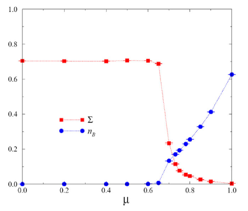
Figure 8.2: Chiral condensate $\Sigma$ and baryon charge density $n_{B}$ as a function of $\mu$ (from [12]).

8.3.2 Diquark Condensation

The diquark condensates $<\psi\psi>$ are calculated in a similar way to the previous expectation values, but this time the derivatives of the partition function are taken with respect to the diquark source (or the anti-diquark source for $<\bar{\psi}\bar{\psi}>$):

$$<\psi\psi>=\frac{1}{V}\frac{\partial\ln Z}{\partial j}$$ (8.44)

In order to effectively study diquark condensation the operators $\psi\psi_{\pm}$ are defined as:

$$<\psi\psi_{\pm}>=\frac{1}{2V}\left(\begin{array}[]{c}\frac{\partial\ln Z}{\partial j}\pm\frac{\partial\ln Z}{\partial\bar{j}}\\ \end{array}\right)$$ (8.45)

with corresponding source strengths $j_{\pm}=j\pm\bar{j}$, so when $j=\bar{j}\Rightarrow j_{-}=0$. Then diquark condensation is given by:

$$<qq_{+}>=\frac{1}{V}\frac{\partial\ln Z}{\partial j_{+}}=\frac{1}{4V}<\textmd{tr}\tau_{2}\mathcal{A}^{-1}>$$ (8.46)

Then, the non-vanishing of (8.46) in the limit $j_{+}\rightarrow 0$ is a criterion for the formation of a diquark condensate and the resulting spontaneous breakdown of the $U(1)_{B}$ symmetry.

Criticality and Superfluidity

However, in [12] it was seen that the diquark condensate does not extrapolate to a non-zero value for high density, but scales non-analytically to zero as

$$<\psi\psi>\propto j^{\frac{1}{\delta}},$$ (8.47)

implying no breakdown of $U(1)_{B}$ symmetry. It was then suggested that this behaviour could be due to working in 2+1 dimensions. The Mermin–Wagner theorem predicts: there can be no phase transition to a state with long-range order at finite temperature for a two dimensional system with a continuous global symmetry[29]. This was supported in [15], where diquark condensation and an energy gap were observed in simulations of the 3+1d NJL model.

It is also seen that the exponent $\delta$ varies continuously with chemical potential, $\mu$, taking the value $\delta\approx 3$ at $\mu=0.8$ and $\approx 5$ at $\mu=0.9$. This suggests a line of critical points for $\mu>\mu_{c}$. This type of behaviour is similar to that observed in other 2-dimensional critical thermodynamic systems. For a spin system (XY model) at its critical temperature the spontaneous magnetisation, $M$, scales with applied magnetic field, $H$, as $M\propto H^{\frac{1}{\delta}}$, where again the exponent forms a line of critical points.

The simplest description of a critical system is given by the XY model, for which long range order would also spontaneously break a $U(1)$ global symmetry. Using this system Kosterlitz and Thouless (KT) described the critical behaviour, of a 2 dimensional system, as a consequence of binding and unbinding of vortex pairs at a critical temperature $T_{KT}$ (Appendix B). Applying this to a 2-dimensional superfluid, the critical temperature is seen to be the point where superfluid vortices bind and unbind. Thus, above the critical temperature when the vortices are free they experience long-rang mutual interactions leading to the behaviour of a viscous fluid; but below the critical temperature vortex-antivortex pairs bind, reducing long range interaction, resulting in superfluid behaviour. The jump from the spin XY model to superfluids comes from the fact that we replace the total spin angle (of vortex-antivortex pairs) in the XY model by the phase angle of the possible superfluid condensate wave function (Appendix B.3). Therefore, (as was conjectured in [12]) in analogy to the non-analytic behaviour displayed by the XY model the high density (and low temperature) critical phase of the 2+1d NJL model can be considered to be a gapless thin film BCS superfluid.

In the rest of this thesis we will investigate this possible superfluid behaviour of 2+1d NJL model. This will be done by extending the baryon density to a baryon three current by the use of Ward Identities. Then, by the use of a spatially varying diquark source we will introduce a gradient in the diquark pair wave function, which should force a flow of the baryon current, and hence result in a measurable signal. Using this current signal we will explore its behaviour (using the helicity modulus, $\Upsilon$, Sec. 9.2) with variations in spatial volume, temperature, and diquark source. We will also attempt to isolate the superfluid (and non-superfluid) states of the 2+1d NJL model with respect to chemical potential and temperature. The variation of superfluidity with respect to temperature will be of most importance. The temperature where superfluidity changes from zero to non-zero should be the critical point of the system, i.e. the point where vortex and antivortex pairs come together to form the superfluid phase. If this critical point of the NJL model coincides with the critical point predicted by the KT theory, this would then be strong evidence that the critical phase of the 2+1d NJL model could be a gapless thin film BCS superfluid.

Chapter 9 Forced Baryon Current Flow

Chiral symmetry restoration of the $2+1$d NJL model is accompanied by the onset of baryon charge density $n_{B}$, as discussed in Sec. 8.3; in the first part of this chapter we will extend this baryon density to a baryon 3-current $I_{\mu}$, where $n_{B}$ is the timelike component, $I_{0}$, of the current. We will then implement a twisted diquark source i.e. a periodically varying source spanning the whole system. In the final section we will then conduct simulations with this twisted source; these will involve comparing the induced baryon 3-current with the constant source to one with a twisted source. We will show that by introducing a twisted source we introduce a diquark phase gradient between the system sites, this then results in a non-zero superfluid current. We will then present the results of the effects on this baryon 3-current, as a result of variations in spatial volume, temperature (i.e changes in temporal volume) and number of cycles of the diquark source.

9.1 Simulating the Baryon 3-Current

In Sec. 8.3 we saw that the baryon charge density is given by:

$$I_{0}\equiv n_{B}\equiv<\bar{\psi}\gamma_{0}\psi>=\frac{1}{V}\frac{\partial\ln Z}{\partial\mu}=<\frac{1}{4V}\textrm{tr}(\mathcal{A}^{-1}\mathcal{X})>$$ (9.1)

This was easily derived, as the NJL lagrangian contains a chemical potential term, which allows simple measurements of the baryon charge density. This charge density can be denoted as the timelike component of a baryon 3-current, which is the conserved Noether current associated with baryon number conservation $U(1)_{B}$, Eqn. (7.13). The association of a conserved Noether current to a global symmetry in continuum field theory has an equivalent in Euclidean quantum field theory: known as the Ward-Takahashi identities. These identities can be derived for a general action (Using the naive fermions):

$$S\sim\frac{1}{2}\sum_{x\nu}(\bar{\psi}_{x}\gamma_{\nu}\psi_{x+\nu}-\bar{\psi}_{x}\gamma_{\nu}\psi_{x-\nu})$$ (9.2)

with a partition function:

$$\mathcal{Z}=\int\mathcal{D}\psi\mathcal{D}\bar{\psi}e^{-S}$$ (9.3)

If this partition function is invariant under a simple $U(1)$ transformation:

$$\psi_{x}\rightarrow\psi_{x}e^{i\alpha}\qquad\bar{\psi}_{x}\rightarrow\bar{\psi}_{x}e^{-i\alpha}$$ (9.4)

we can derive the Ward-Takahashi identities, and hence the conserved currents of the symmetry. Under the $U(1)$ transformation, the above action becomes:

$$S\rightarrow\frac{1}{2} \sum_{x\nu} [e^{-i\alpha}(\bar{\psi}_{x}\gamma_{\nu}\psi_{x+\nu}-\bar{\psi}_{x}\gamma_{\nu}\psi_{x-\nu})$$ (9.5)

$$+ e^{i\alpha}(\bar{\psi}_{x-\nu}\gamma_{\nu}\psi_{x}-\bar{\psi}_{x+\nu}\gamma_{\nu}\psi_{x})]$$

which can be written as $S\rightarrow S+\delta S$, where

$$\delta S\sim- \frac{i\alpha}{2} [(\bar{\psi}_{x+\nu}\gamma_{\nu}\psi_{x}+\bar{\psi}_{x}\gamma_{\nu}\psi_{x+\nu})$$ (9.6)

$$- (\bar{\psi}_{x}\gamma_{\nu}\psi_{x-\nu}+\bar{\psi}_{x-\nu}\gamma_{\nu}\psi_{x})]+\mathcal{O}(\alpha^{2})$$

$$= -i\alpha\nabla_{\nu}^{-}I_{\nu}(x)$$

where the final line, known as the Ward identity, is written in terms of the backwards operator,$\nabla_{\nu}^{-}$, and $I_{\nu}(x)$ is given as:

$$I_{\nu}(x)=\frac{1}{2}(\bar{\psi}_{x+\nu}\gamma_{\nu}\psi_{x}+\bar{\psi}_{x}\gamma_{\nu}\psi_{x+\nu})$$ (9.7)

This can be shown to be the conserved current of the $U(1)$ symmetry, by writing the transformed partition function as:

$$\mathcal{Z}^{\prime} = \int\mathcal{D}\psi^{\prime}\mathcal{D}\bar{\psi}^{\prime}e^{-S(\psi^{\prime},\bar{\psi}^{\prime})}e^{-\delta S(\psi^{\prime},\bar{\psi}^{\prime})}$$ (9.8)

$$= \int\mathcal{D}\psi^{\prime}\mathcal{D}\bar{\psi}^{\prime}(1-i\alpha\nabla_{\nu}^{-}I_{\nu}(x))e^{-S(\psi^{\prime},\bar{\psi}^{\prime})}$$

$$= \mathcal{Z}$$

$$\Rightarrow <\nabla_{\nu}^{-}I_{\nu}(x)>=0$$

The last line shows a zero expectation value of the Ward identity. This then implies that the current $I_{\nu}(x)$ is conserved.

Now the conserved current in Eqn. (9.7) can be used to determine the current components $I_{1}$ and $I_{2}$ associated with the $U(1)_{B}$ global symmetry. In order to do this we can compare our NJL action, Eqn. (8.16) and (8.19), with the above action, Eqn. (9.2), so we can write the Ward current components for our NJL model as:

$$I_{0}(x) = \frac{1}{2}(e^{\mu}\bar{\chi}_{x}\chi_{x+\hat{0}}+e^{-\mu}\bar{\chi}_{x}\chi_{x-\hat{0}})$$

$$I_{i}(x) = \frac{1}{2}(\eta_{i}\bar{\chi}_{x}\chi_{x+\hat{i}}+\eta_{i}\bar{\chi}_{x}\chi_{x-\hat{i}})$$ (9.9)

where $i=1,2.$ Now comparing the $I_{0}$ component with the baryon charge density expectation value, Eqn. (8.43), we can adjust the matrix (LABEL:baryon_x_matrix) to correspond with the $I_{i}$ components. Then the equivalent matrix for the $I_{i}$ components is given by:

$$\mathcal{X^{\star}}_{i}=\frac{1}{4}\left(\begin{array}[]{cc}0&\delta^{pq}\eta_{i}[\delta_{y,x+\hat{i}}+\delta_{y,x-\hat{i}}]\\ \delta^{pq}\eta_{i}[\delta_{y,x-\hat{i}}+\delta_{y,x+\hat{i}}]&0\\ \end{array}\right)$$ (9.10)

where the expectation value of the baryon current density, $I_{i}$, are given as:

$$I_{i}\equiv<\bar{\psi}\gamma_{i}\psi>=<\frac{1}{4V}\textrm{tr}(\mathcal{A}^{-1}\mathcal{X^{\star}}_{i})>$$ (9.11)

where $i=1,2$.

9.2 Introducing the Twisted Diquark Source

Previous simulations, as in [12], were conducted using a constant diquark source,

$$j\psi\psi+\bar{j}\bar{\psi}\bar{\psi}$$ (9.12)

where $j=\bar{j}=j_{0}$. This was sufficient to force diquark condensation and derive physically meaningful results in the limit $j\rightarrow 0$. Such simulations have shown, as the Mermin-Wagner theorem states, there is no observable diquark condensation for the $2+1$d NJL system. However, the diquark condensate behaves in a non-analytic way, which could imply the existence of a type of superfluid phase at high density (discussed in Sec. 8.3.2). Such a two dimensional superfluid state, without an obvious diquark condensation phase, can be associated with the binding [and unbinding] of vortex pairs that leads to the critical phase, as in the XY model (Appendix B). For our NJL system the vortices can be associated with the phase of the current carrying superfluid particles, i.e. the phase of the diquark pairs:

$$<\psi\psi>(\vec{x})=\varphi(\vec{x})_{diquark}=\varphi_{0}\exp(i\theta(\vec{x}))$$ (9.13)

Where $\theta(\vec{x})$ is the phase corresponding to the external diquark source; where for a constant real source, as used in [12], the phase is $\theta=0$.

We can now substitute Eqn. (9.13) into the current density:

$$\vec{I}\sim(\varphi\vec{\nabla}\varphi^{*}-\varphi^{*}\vec{\nabla}\varphi),$$ (9.14)

which will give us the baryon current density over the $x$-$y$ plane, i.e. the components $I_{1}$ and $I_{2}$:

$$\vec{I}=\Upsilon\vec{\nabla}\theta(\vec{x}),$$ (9.15)

where $\Upsilon$ is defined as the constant of proportionality between the current density and the gradient of the phase of the superfluid components, $\Upsilon=(\phi_{0})^{2}$, and is known as the helicity modulus(Appendix B)[38]. From this we can see that using the constant source above, or a complex constant diquark source:

$$j=j_{0}\exp(i\theta)\qquad\bar{j}=j_{0}\exp(-i\theta)\textrm{,}$$ (9.16)

where $\theta$ is a real constant, we have no gradient over the $x$-$y$ plane:

$$\vec{\nabla}\theta=0$$ (9.17)

This zero gradient leads to a zero current density. For this reason, we must implement a source that generates a non zero gradient over the $x$-$y$ plane, which would then lead to a spatially varying diquark wave function, which in turn implies a non-zero current density. If we introduce a "twisted" (or periodic) source:

$$j=j_{0}\exp(i\theta(\vec{x}))\qquad\bar{j}=j_{0}\exp(-i\theta(\vec{x}))$$ (9.18)

where the phase, dependent on spatial position, is given as:

$$\theta(\vec{x})=2\pi\frac{x_{1}}{L_{1}}+2\pi\frac{x_{2}}{L_{2}}$$ (9.19)

then, depending on the direction of the twist, this leads to a non-zero current density, given by inserting (9.19) into (9.15):

$$I_{1}=\Upsilon\frac{2\pi}{L_{1}}\qquad I_{2}=\Upsilon\frac{2\pi}{L_{2}}$$ (9.20)

So, in an attempt to force a superfluid current flow, we implemented a generalised version of (9.18),

$$j=j_{0}\exp(i2\pi n_{1}\frac{x_{1}}{L_{1}})\qquad\bar{j}=j_{0}\exp(-i2\pi n_{2}\frac{x_{2}}{L_{2}})$$ (9.21)

where $n_{1}$ and $n_{2}$ are the number of cycles in the source spanning the lattice. Thus, similarly to (9.20), the baryon current should become:

$$I_{1}=\Upsilon\frac{2\pi}{L_{1}}n_{1}\qquad I_{2}=\Upsilon\frac{2\pi}{L_{2}}n_{2}$$ (9.22)

Also, as the baryon charge density would only depend on the magnitude of the diquark source, the signal for $I_{0}$ should be unaffected with this twisting of the source.

9.3 Simulations of the 3-current

Running simulations, as is often the case, is a time consuming task. Each run of the Hybrid Molecular Dynamics (HMD) code, with particular magnitudes of diquark source $|j|=j_{0}$ and density (chemical potential) $\mu$, generates results for one value of $\vec{I}$. So, in order to create a plot of baryon current as a function of $j$ with 9 points, we had to run 9 simulations - for one particular value of chemical potential. Then, to plot the extrapolated value of baryon current (as $j\rightarrow 0$) as a function of $\mu$, with 10 points, would mean we need to run 90 simulations. Taking into account the fact that these simulations were conducted with variations in spatial dimensions $L_{s}$ (to study finite volume effects) and variations in the temporal dimension $L_{t}$ (to study effects due to temperature variation), we were looking at over 1000 runs. So in an attempt to eliminate unnecessary runs we conducted our study in two parts. This section represents the preliminary study of the superfluid phase. Here we start off first by testing the baryon three current with the twisted source. Then we go on to study the general thermodynamic behaviour of the superfluid state; that is, we analyse how the baryon current behaves at high and low temperatures and chemical potentials, without running detailed simulations in the intermediate transition period. In this way, if we see a jump in the superfluid current from high temperature to low temperature, we could then go and study the transition period, and relate it to the $KT$ transition as described by the XY model. Then in a similar way we could study the effect of the current with respect to changes in chemical potential.

Physical Units

The simulations in this work were conducted with a strong coupling $g^{2}=2.0$ corresponding to $\Sigma a=0.71$, as in [12]; where the result $\Sigma a$ is the dimensionless measure of the constituent quark mass. In the same way our measurements of the helicity modulus, from the HMD simulations, will be in the dimensionless form $\Upsilon=\Upsilon_{0}a$, determined by a straight line extrapolation of the baryon current against diquark source. Therefore, in order to obtain physically meaningful results we will need to take the ratio:

$$\frac{\Upsilon_{0}}{\Sigma}=\frac{\Upsilon_{0}a}{\Sigma a}=\frac{\Upsilon}{0.71}$$ (9.23)

This will become necessary in Chapter. 10, when we relate our measured value of $\Upsilon$ to temperature.

9.3.1 Constant and Twisted Diquark Source

In Fig. 9.1 we have plotted all the components of the baryon 3-current as a function of the constant diquark source $j=\bar{j}=j_{0}$. In this plot it can be seen that the only non zero parts are the baryon charge density $I_{0}$. This is as we expected, as the constant source produces no gradient, hence there is no superfluid baryon current flow, i.e. $I_{1}=I_{2}=0$.

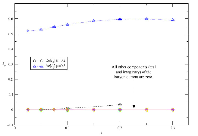
Figure 9.1: Real and Imaginary parts of the baryon 3-current, $I_{\mu}$, as a function of constant diquark source, $j$. (Lattice Size=$16\times 16\times 64$)

In Fig. 9.2 we have plotted the non-zero components of the baryon 3-current with the twisted diquark source (9.21). We conducted two sets of simulation, the first was with the source only twisted in the $x$ direction, and the second with the source only twisted in the $y$ direction. We found, as expected, that for a twist in the $x$ direction we had a super current signal $I_{1}\neq 0$ and for a twist in the $y$ direction we had a signal $I_{2}\neq 0$. These simulations were conducted for the same magnitudes of the diquark source, so that both simulations gave the same signal for the baryon charge density $I_{0}=n_{B}$.

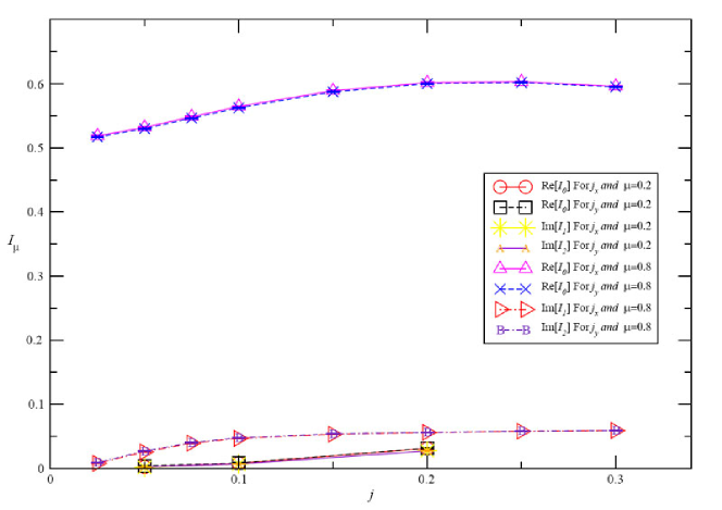
Figure 9.2: Non-zero components of baryon 3-current, $I_{\mu}$, as a function of twisted diquark source $j_{\mu}$, with $n_{1}=n_{2}=1$. (Lattice Size=$16\times 16\times 64$)

It is also seen that the signals generated for the super currents $I_{1}$ and $I_{2}$ are identical; this is obvious from eqn. 9.22 if we have $L_{1}=L_{2}$ and $n_{1}=n_{2}$. Therefore in the rest of the simulations we only conducted simulations for a twist in the $y$ direction, and assumed that a twist in the $x$ direction would give identical results.

9.3.2 Twisted Source with n-Cycles

We conducted simulations to test how the baryon current, $I_{2}$, changed as we varied the number of cycles (or twists) in the diquark source, $n_{2}$. This was done for high and low chemical potential $\mu=0.8$ and $0.2$, and the results have been plotted in Fig. 9.3.

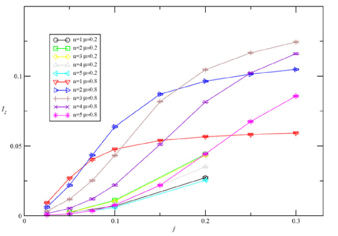
Figure 9.3: Baryon current, component $I_{2}$, as a function of twisted diquark source, $j_{2}$, for various values of $=n_{2}$. (Lattice Size=$16\times 16\times 24$)

You can note that as you increase the number of cycles for the low chemical potential, $\mu=0.2$, the $I_{\mu}\propto j^{2}$ behaviour, which is more prominent in Figs. 9.6 and 9.7, becomes more pronounced.

However, at high $\mu$, the behaviour shifts from an approximate linear fit ($I_{\mu}\propto j$) to a parabolic fit ($I_{\mu}\propto j^{2}$). This shift then leads to a zero extrapolation of the baryon current as $j\rightarrow 0$. So as you increase the number of cycles the baryon current ceases to flow. This shift and the resulting destruction of the baryon current can be considered due to finite volume effects. From Eqn. (9.22) it can be seen that increasing $n$ from $1$ to $2$ cycles has an effect of decreasing the wavelength from $L$ to $L/2$. Therefore, increasing the lattice size would counteract the effect of increasing the number of cycles. This can be seen in Fig. 9.4 where we have plotted the baryon current, $I_{2}$, against diquark source with $n=2$ cycles. We have also plotted the a baryon current for $n=1/2$. However, due to periodic boundary conditions the results for non-integer values of $n$ do not coincide with those of the physically relevant current signals, corresponding to integer values of $n$. This is seen clearly from the plots for $L_{s}=16,n=0.5$ and $L_{s}=32,n=1$, in Fig. 9.4.

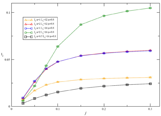
Figure 9.4: Baryon current, component $I_{2}$, as a function of twisted diquark source, $j_{2}$, for $=n_{2}=1$, $2$ and $0.5$ and lattice size $L_{s}=16$, $32$, and $L_{t}=24$

It can also be noted that by using different size spatial dimensions we obtain very different baryon currents, so the baryon current is dependent on the spatial lattice size. In order to obtain a result that is independent of spatial dimensions, we need to work with the helicity modulus, which will only vary depending on spatial size as a result of finite volume effects. The use of the Helicity modulus will be discussed in further detail in Sec. 9.4.

9.3.3 Effects of Temperature and Density Variation

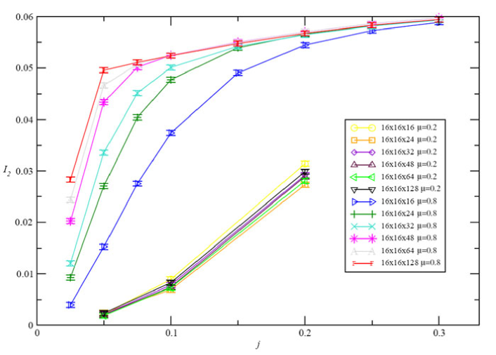
Figure 9.5: Baryon current, $I_{2}$, as a function of twisted diquark source, $j$, for various time dimensions and fixed space, $L_{s}=16$.

In Fig. 9.5 we have plotted the baryon current, $I_{2}$, as a function of diquark source, for a fixed spatial volume ($L_{s}=16$), two values of chemical potential and various time dimensions ($L_{t}$). At low chemical potential, $\mu=0.2$, it can be seen that there is not much variation in $I_{2}$ with changes in temperature $(T=1/L_{t})$. However, at high chemical potential, $\mu=0.8$, the current can be seen to collapse onto a straight line as you decrease temperature. By $L_{t}=128$ it becomes clear that $I_{2}$ extrapolates to a non-zero value as $j\rightarrow 0$. From these results we decided to conduct further simulations using $L_{t}=64$, as this gives us results comparable to $L_{t}=128$, however in a third of the CPU time.

In Fig. 9.6 we have plots of various $\mu$ at low temperature ($L_{t}=64$). It can be seen that the current behaves in a fundamentally different way at high density ($\mu\geq 0.68$) compared to low density ($\mu\leq 0.65$). As we go from high to low $\mu$ the negative curvature of the high density phase shifts sharply to a strong quadratic type, which can then be extrapolated to $I_{2}=0$. In this way we can determine the critical chemical potential for the onset of superfluidity as $0.65<\mu_{c}<0.68$, which is also the region of chiral symmetry restoration i.e. $\mu_{c}\sim 0.65$ (Fig. 8.2). On the other hand, it can be seen from Fig. 9.7 that at high temperature ($L_{t}=4$), all the chemical potential curves follow a quadratic extrapolation to $I_{2}=0$ at $j=0$. So, at high temperature no superfluid state exists.

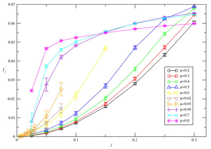
Figure 9.6: Baryon current, $I_{2}$, as a function of twisted diquark source, $j$, for various chemical potential ($\mu$) at low temperature ($L_{t}=64$). ($L_{s}=16$)

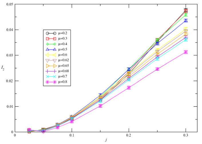
Figure 9.7: Baryon current, $I_{2}$, as a function of twisted diquark source, $j$, for various chemical potential ($\mu$) at high temperature ($L_{t}=4$). ($L_{s}=16$)

Also, even though we have a possible linear extrapolation for the low temperature and high density phase, as seen in Fig. 9.5 (for $L_{t}=128)$, we do not have a systematic method of extrapolating to $j\rightarrow 0$ for $\mu\geq\mu_{c}$ in general, therefore we are unable to make any decisive statement about the nature of the transition.

$I_{2}$ as a Function of $j$

The behaviour of the baryon current, $I_{2}$, as a function of source, $j$, can be summarised as:

$$I_{2}(j,\mu,T)=I_{2}(0,\mu,T)+A(\mu,T)j+B(\mu,T)j^{2}$$ (9.24)

At low temperature, and for high $\mu$ (as for the case $\mu=0.8$ in Figs. 9.5  and 9.6) we have: $B=0$ and $A\neq 0$, and a possible straight line fit extrapolates (as $j\rightarrow 0$) to $I_{2}(0,\mu)\neq 0$. However, for low $\mu$ (as for $\mu\leq 0.65$ in Fig. 9.6) we have: $A=0$ and $B\neq 0$ which leads to a $j^{2}$ fit, extrapolating (as $j\rightarrow 0$) to $I_{2}(0,\mu)=0$. On the other hand, at high temperature this behaviour changes (Fig. 9.7), here the extrapolation is of the form $j^{2}$ for all values of $\mu$, i.e. $I_{2}(0,\mu,T)=A(\mu,T)=0$. The extrapolation shift from $j$ to $j^{2}$ can be understood if we have different wave functions for the current carrying superfluid particles at different chemical potentials:

$$\phi(\vec{x}) = \phi_{0}j_{0}\exp(i\theta(\vec{x}))\qquad\mu<\mu_{c}$$

$$\phi(\vec{x}) = \phi_{0}\exp(i\theta(\vec{x}))\qquad\mu>\mu_{c}$$ (9.25)

The linear $j_{0}$ dependence, at low chemical potential, is expected due to the fact that there should be no diquark condensate for $\mu<\mu_{c}$; so $\phi\rightarrow 0$ as $j\rightarrow 0$. In this way, using Eqn. (9.14), the baryon current is:

$$\vec{I} \sim \phi_{0}^{2}j_{0}^{2}\vec{\nabla}\theta(\vec{x})\qquad\mu<\mu_{c}$$

$$\vec{I} \sim \phi_{0}^{2}\vec{\nabla}\theta(\vec{x})\qquad\mu>\mu_{c}$$ (9.26)

and in the limit $j\rightarrow 0$, we have:

$$\vec{I} \sim 0\qquad\mu<\mu_{c}$$

$$\vec{I} \sim \phi_{0}^{2}\vec{\nabla}\theta(\vec{x})=\textrm{constant}\qquad\mu>\mu_{c}$$ (9.27)

which is the behaviour of the baryon current as seen throughout our simulations.

9.4 Finite Volume Effects

We have, so far, been working with the baryon current, $I_{2}$, for example in Fig. 9.6 we have plotted the current against diquark source. However, this is not the most appropriate variable to work with, due to its dependence on spatial volume, as we saw briefly in Sec. 9.3.2. This dependence on spatial volume can be seen clearly when we conduct simulations for a fixed temperature, but differing spatial sizes: in Fig. 9.8 it can be seen that, at low temperature, the baryon current differs hugely for the three different spatial volumes $L_{s}=16$, $24$ and $32$, and any linear extrapolation of the baryon current with $j\rightarrow 0$ will give very different results. However, at low $\mu$ and/or high temperature, when the extrapolation is of the $j^{2}$ form, finite volume effects do not matter too much as all extrapolations tend to $I_{2}\rightarrow 0$, Figs. 9.8 and 9.9.

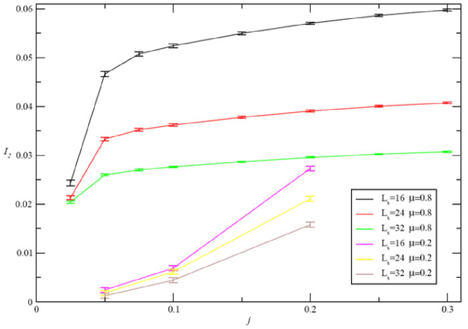
Figure 9.8: Baryon current, $I_{2}$, as a function of twisted diquark source, $j$, for various spatial dimensions, $\mu=0.2$ and $0.8$, and low temperature, $L_{t}=64$.

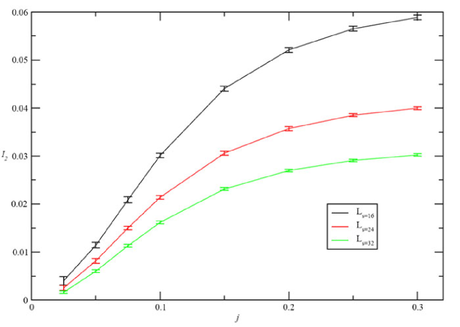
Figure 9.9: Baryon current, $I_{2}$, as a function of twisted diquark source, $j$, for various space dimensions, $\mu=0.8$, and high temperature, $L_{t}=12$.

9.4.1 Working with the Helicity Modulus

We can overcome effects of spatial dependence by working with the helicity modulus, $\Upsilon$, which, as seen earlier, is the constant of proportionality between the baryon current and the gradient of the source’s phase, Eqn. (9.15). In this way we are able to represent, in a volume independent manner, the superfluid behaviour of the system. So, when we plot $\Upsilon=I_{2}L_{s}/2\pi$ against $j$ for varying spatial volumes, $L_{s}$, but constant temperature and chemical potential, any variations in the plots could be put down to finite volume effects.

Low Temperature Finite Volume Effects

In Fig. 9.10 we have plotted $\Upsilon$ against $j$ for low temperature, $L_{t}=64$; this is only done for high $\mu$, as for lower values of $\mu$ the extrapolation is always of the $j^{2}$ type, which implies the current, and thus, the helicity modulus extrapolates to zero as $j\rightarrow 0$.

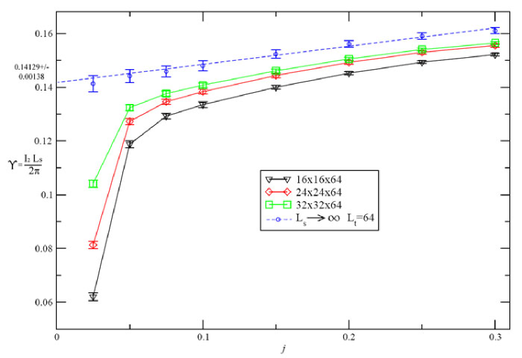
Figure 9.10: Helicity modulus, $\Upsilon$, as a function of twisted diquark source, $j$, for various spatial dimensions, $\mu=0.8$ and low temperature, $L_{t}=64$.

We can note that the dip in $\Upsilon$, at low $j$, decreases as the spatial volume increases; thus, if this dip is a finite volume effect it should tend to a straight line in the infinite volume. In order to analyse this dip at larger volumes, we extrapolated $\Upsilon$ to the limit of $L_{s}\rightarrow\infty$ by plotting $\Upsilon$ for each value of $j$ against $1/L_{s}$, Fig. 9.11, and then the infinite volume value of $\Upsilon$ was deduced by extrapolating the plots $1/L_{s}\rightarrow 0$. The infinite volume plot of $\Upsilon$ is also plotted in Fig. 9.10; and it can be seen that the dip vanishes in this limit, hence this effect can be put down to finite volume effects.

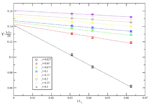
Figure 9.11: Helicity modulus, $\Upsilon$, as a function of $1/L_{s}$, for various $j$, $\mu=0.8$ and low temperature, $L_{t}=64$.

From the low temperature, infinite volume plot, we have conducted an extrapolation of $\Upsilon$ for $j\rightarrow 0$, which should represent the dimensionless value of $\Upsilon$ at low temperature: $\Upsilon=0.1413\pm 0.0014$.

High Temperature Finite Volume Effects

Using the same techniques as before we studied the superfluid behaviour at high temperature, $L_{t}=4$. In Fig. 9.12 we have plotted $\Upsilon$ for $\mu=0.8$, $L_{t}=4$ and, again, for various spatial volumes. As before we extrapolate to the infinite volume limit, where the extrapolation lines are shown in Fig. 9.13.

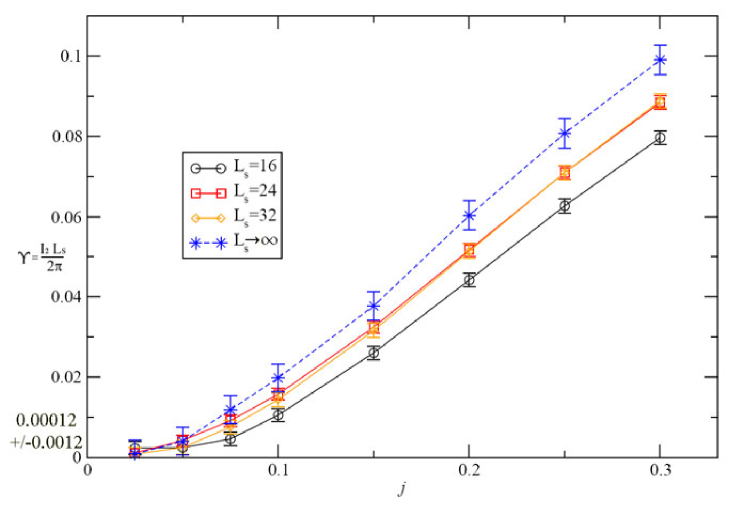
Figure 9.12: Helicity modulus, $\Upsilon$, as a function of twisted diquark source, $j$, for various spatial dimensions, $\mu=0.8$ and high temperature, $L_{t}=4$.

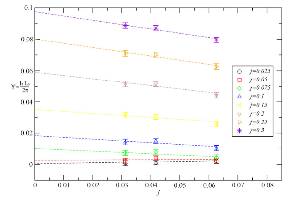
Figure 9.13: Helicity modulus, $\Upsilon$, as a function of $1/L_{s}$, for various $j$, $\mu=0.8$ and high temperature, $L_{t}=4$.

In Fig. 9.12 we have also plotted the curve for $L_{s}\rightarrow\infty$. From this we see that at high temperature and in the infinite volume limit the $\Upsilon\propto j^{2}$ behaviour does not change significantly, if anything it becomes more pronounced at lower values of $j$. From this extrapolation we find $\Upsilon=0.00012\pm 0.0012\sim 0$.

Behaviour at Intermediate Temperature

We have shown that at low temperature there are significant, but controllable, finite volume effects, which are removed by extrapolating to the infinite volume limit. In the infinite volume limit the low temperature linear behaviour, $\Upsilon(j)\propto\Upsilon(0)+Aj$, becomes obvious and straight line extrapolations for $j\rightarrow 0$ lead to $\Upsilon\neq 0$. At high temperature, where we expect a $\Upsilon(j)\propto j^{2}$ behaviour, working on a finite volume does not have much of an effect, that is the finite volume plots do not differ from the infinite volume extrapolation. So, we can state that the superfluid current drops from a non-zero value at low $T$ to a zero value at high $T$.

However, if we attempt to analyse the intermediate temperature region we encounter some difficulties. In Fig. 9.14 we have plotted $\Upsilon$ for $\mu=0.8$, $L_{t}=12$.

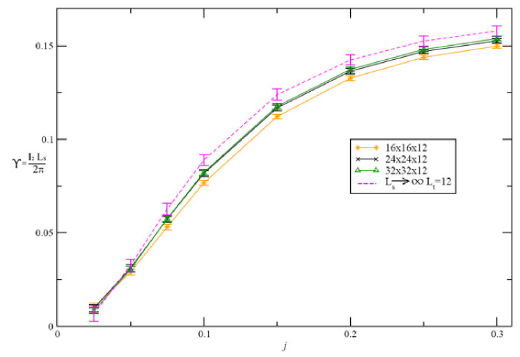
Figure 9.14: Helicity modulus, $\Upsilon$, as a function of twisted diquark source, $j$, for various spatial dimensions, $\mu=0.8$ and high temperature, $L_{t}=12$.

The extrapolation of this, to the thermodynamic limit, is given in Fig. 9.15. We see that the various volume plots have an "s" shaped form, which remains even in the infinite volume limit.

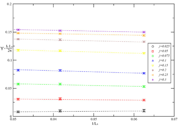
Figure 9.15: Helicity modulus, $\Upsilon$, as a function of $1/L_{s}$, for various $j$, $\mu=0.8$ and high temperature, $L_{t}=12$.

In this case we could implement a $j^{2}$ extrapolation for the first four points, however this does not seem very conclusive as the last 4 points lie well outside any $j^{2}$ behaviour. On the other hand, in Fig. 9.16, where we have again plotted a curve for $L_{t}=12$, but now we have used a larger volume, $(L_{s}=40)$, and obtained further points at low $j$, a $j^{2}$ extrapolation does seem appropriate. From this extrapolation $\Upsilon$ can be deduced to be $\Upsilon=0.00016\pm 0.0014\sim 0$.

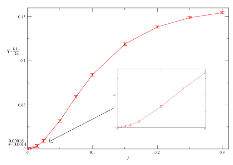
Figure 9.16: Helicity modulus, $\Upsilon$, as a function of twisted diquark source, $j$, for $L_{s}=40$, $\mu=0.8$ and high temperature, $L_{t}=12$.

A similar situation occurs as you decrease the temperature further. In Fig. 9.17 we have a plot of $L_{t}=24$, and its extrapolation lines in Fig. 9.18. At this temperature we can see that it is not obvious if this plot falls under a linear extrapolation (giving $\Upsilon\neq 0$) or a parabolic extrapolation (giving $\Upsilon=0$). At low $j$ the curve must tend to $\Upsilon=0$ hence it must follow a $j^{2}$ curve to the origin. But, more plausibly, we could apply a straight line extrapolation to the last 5 points. Even in the infinite volume limit it does not obviously fall under either extrapolation criteria.

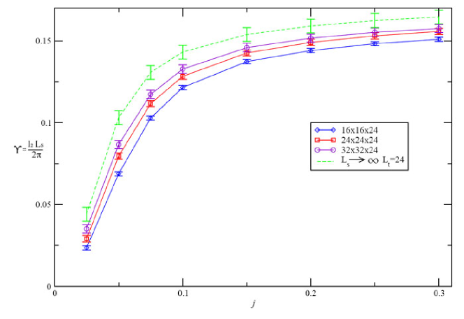
Figure 9.17: Helicity modulus, $\Upsilon$, as a function of twisted diquark source, $j$, for various spatial dimensions, $\mu=0.8$ and temperature, $L_{t}=24$.

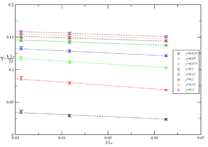
Figure 9.18: Helicity modulus, $\Upsilon$, as a function of $1/L_{s}$, for various $j$, $\mu=0.8$ and temperature, $L_{t}=24$.

In the next chapter we will go on to investigate the intermediate temperature range. We will attempt to deduce some criterion for the extrapolation of these temperatures, which will then help in isolating the critical temperature i.e. the temperature at which $\Upsilon$ falls from the non-zero superfluid value at low $T$ to a zero value in the non-superfluid phase at high $T$.

Chapter 10 Thin Film Superfluid Dynamics

In the previous chapter it was shown that the baryon current-density has a strong transition in the region $0.65<\mu_{c}<0.68$ - the region corresponding to chiral symmetry restoration. Also, working with the spatially independent helicity modulus, $\Upsilon$, it was shown that at low temperature, $L_{t}=64$, and high chemical potential, $\mu=0.8$, the helicity modulus extrapolates to $\Upsilon=0.1413\pm 0.0014$; and at high temperature, $L_{t}=4$, it extrapolates to zero. However, at intermediate temperatures, for example $L_{t}=12$ and $L_{t}=24$, extrapolation techniques are not obvious - even in the infinite volume limit. In this chapter we will investigate the behaviour of $\Upsilon$ in this intermediate region, and attempt to provide some extrapolation criteria for this puzzling domain. The aim of this chapter will be to try and isolate the critical temperature and see if it corresponds with the predicted $T_{KT}$ temperature, given by the theory of Kosterlitz and Thouless (KT).

10.1 $T_{KT}$ given by Kosterlitz and Thouless’ Theory

If the phase transition, for the 2+1d NJL model at high density, is described by the KT theory (Appendix B) then the critical temperature should be given by Eqn. (B.23), or in lattice units:

$$aL_{t}=\frac{1}{T_{KT}}=\frac{2}{\pi}\frac{1}{\Upsilon_{0}}\qquad\rightarrow\qquad L_{t}=\frac{1}{aT_{KT}}=\frac{2}{\pi}\frac{1}{\Upsilon},$$ (10.1)

where $\Upsilon=\Upsilon_{0}a$ is the dimensionless measured value. Using our value of $\Upsilon$ we find:

$$L_{t}=\frac{2}{\pi}\frac{1}{0.14129\pm 0.00138}=4.51\pm 0.44$$ (10.2)

Therefore, according to the KT theory the critical $L_{t}$ should be approximately $6$, which is the nearest even lattice length where the fluid phase jumps to that of a superfluid state. This implies that everything above (and including) this critical length (temperature) should be in the superfluid phase (the bound vortex phase)i.e. $\Upsilon\neq 0$. This suggests that the $L_{t}=6$ data should follow a linear extrapolation to the origin. However, from our previous findings it was shown that $L_{t}=12$ follows more of a $j^{2}$ extrapolation than a linear one, but even this is not very clear. We will now investigate the intermediate domain, ranging from $L_{t}=6-64$, in order to determine, whether or not, the KT critical point exists in our $2+1d$ NJL model.

10.2 Extrapolation Criteria and the Critical Point

In order to investigate the change in $\Upsilon$ from the high temperature ($\Upsilon(j)\propto j^{2}$) phase to the low temperature linear ($\Upsilon(j)\propto\Upsilon(0)+Aj$) phase we have plotted, in Fig. 10.1, $\Upsilon$ against $j$ for temperatures ranging from $L_{t}=2$ to $L_{t}=64$.

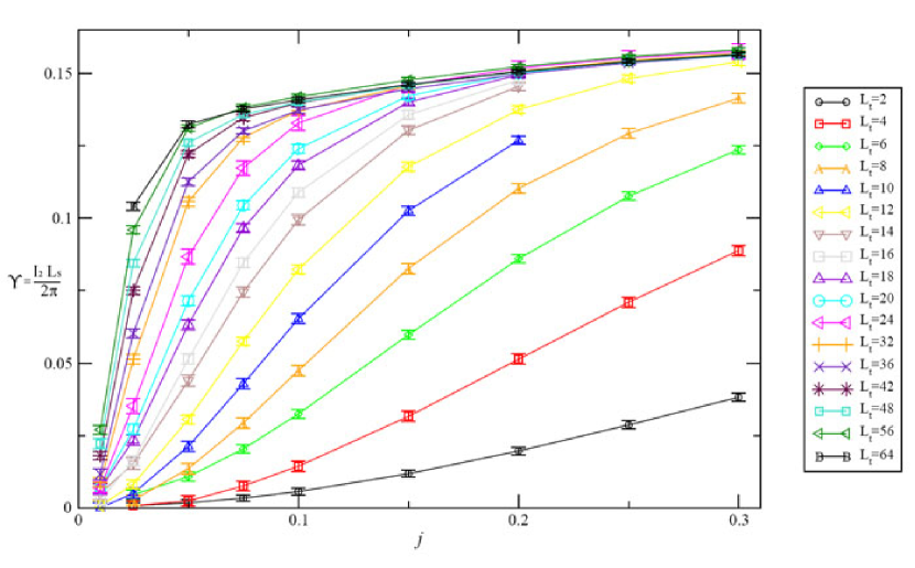
Figure 10.1: $\Upsilon$ as a function of $j$ for various $L_{t}$ ($\mu=0.8$ and $L_{s}=32$).

In this plot we can see a steady transition from the obvious $j^{2}$ form at $L_{t}=2$ to an "s" shaped form between $L_{t}=6-24$ and a straight line form above $L_{t}=24$ (which dips to the origin at low $j$). From this we cannot really distinguish any real, abrupt, phase change. So, to obtain a different perspective we have plotted the same data as $\Upsilon$ against $L_{t}$ for the various $j$ values in Fig. 10.2; and in Fig. 10.3 we have a more detailed plot of the $j=0.025$ data.

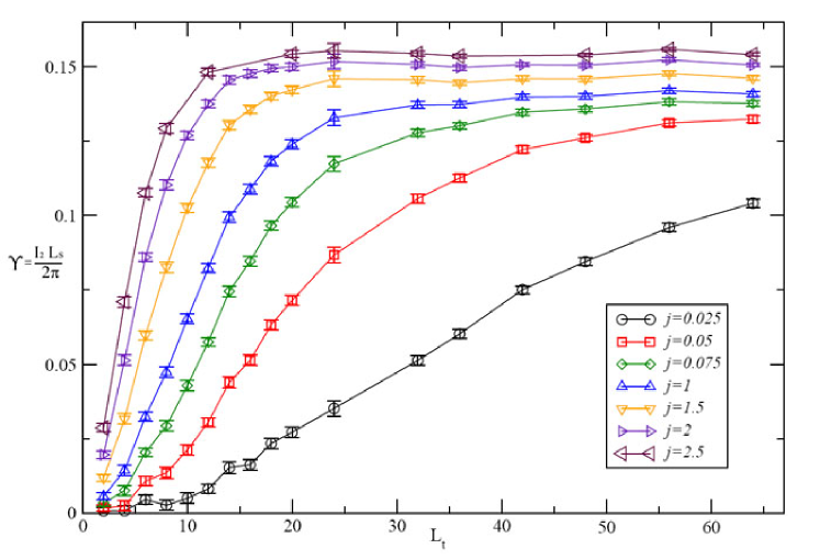
Figure 10.2: $\Upsilon$ as a function of $L_{t}$ for various $j$ ($\mu=0.8$ and $L_{s}=32$).

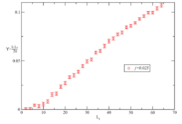
Figure 10.3: A detailed plot of $\Upsilon$ as a function of $L_{t}$ for $j=0.025$ ($\mu=0.8$ and $L_{s}=32$).

From Fig. 10.2 we can see that $\Upsilon$ decreases steadily from $L_{t}=64$ to $L_{t}=24$, for $j>0.025$. However, below $L_{t}=24$ it drops drastically to $\Upsilon=0$. For $j=0.025$, in Fig. 10.3, it can be seen that $\Upsilon$ follows almost a straight line. In Fig. 10.4 we have conducted a straight line extrapolation to $\Upsilon=0$, from which we found $L_{t}=5.54\pm 1.66$.

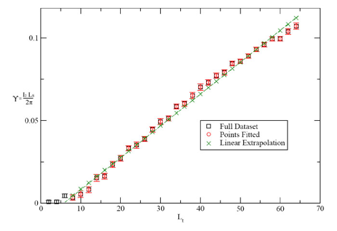
Figure 10.4: $\Upsilon$ as a function of $L_{t}$ for $j=0.025$ with extrapolation line $y=a_{0}x+a_{1}$ ($a_{0}=0.00192\pm 0.0005$ and $a_{1}=-0.01062\pm 0.0015$); ($\mu=0.8$ and $L_{s}=32$).

Also, in Fig. 10.5 we have conducted another extrapolation, of the same data, but now with only the first 18 points; from which we find: $L_{t}=7.24\pm 0.9$. From these two fits we have the average: $L_{t}=6.4\pm 1.9$. This value of $L_{t}$ is comparable to the one derived in Eqn. (10.2). Therefore, we could conjecture that the critical KT temperature could be described by the point where $\Upsilon$ intersects the $L_{t}$ axis for a fixed small $j$. In order to confirm this we would need to conduct further simulations using smaller $j$ (e.g. $j=0.01$) and maybe larger volumes (in order to reduce finite volume effects).

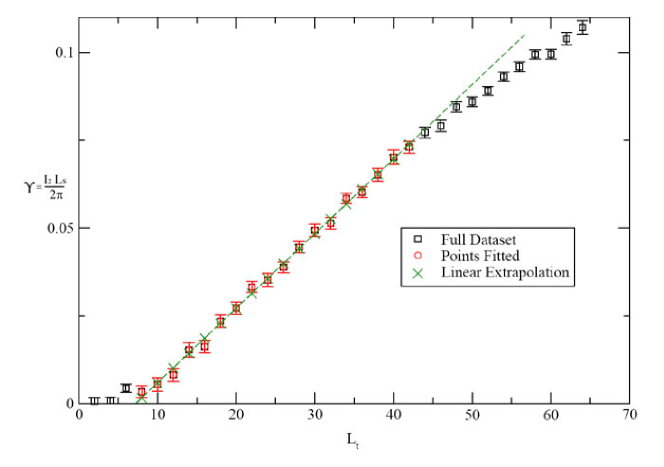
Figure 10.5: $\Upsilon$ as a function of $L_{t}$ for $j=0.025$ with extrapolation line $y=a_{0}x+a_{1}$ using only 18 points ($a_{0}=0.002124\pm 0.00025$ and $a_{1}=-0.015367\pm 0.0009$); ($\mu=0.8$ and $L_{s}=32$).

10.2.1 Finite Volume Effects at Low Temperature

Even though we have located a possible candidate for the critical temperature, it still does not provide any obvious extrapolation criterion for the range $L_{t}=6-24$.

Our next task will be to find a definite lower limit for the superfluid state, i.e. the smallest $L_{t}$ point for which infinite volume extrapolations eliminate the dip in $\Upsilon$ at low $j$. As for $L_{t}=64$, Fig. 9.10, we conducted similar extrapolations for $\Upsilon$ down to $L_{t}=48$. It was found that the dip at low $j$ disappears for extrapolations down to $L_{t}=56$, Fig. 10.6; these simulations were only done for $4$ points, at low values of $j$, in order to reduce time.

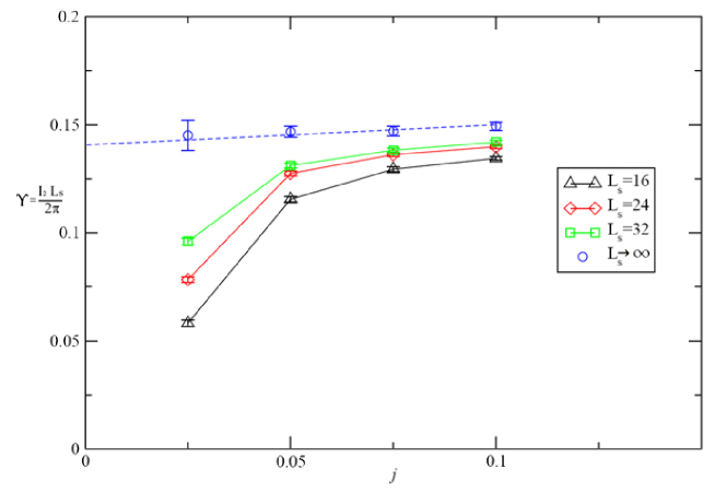
Figure 10.6: The first $4$ points of $\Upsilon$ as a function of $j$ for $L_{t}=56$ ($\mu=0.8$ and $L_{s}=32$).

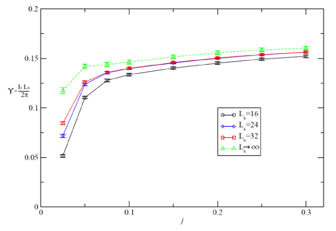
Figure 10.7: $\Upsilon$ as a function of $j$ for $L_{t}=48$ ($\mu=0.8$ and $L_{s}=32$).

So, down to and including $L_{t}=56$ the dip at low $j$ vanishes in the infinite volume limit. However, below this point the dip becomes more and more pronounced, even in the infinite volume limit, Fig. 10.7. As can be seen for $L_{t}=24$, Fig. 9.17, the dip eventually becomes something that you cannot just ignore.

As in the previous chapter, the infinite volume limit extrapolations for $L_{t}=48$ and $L_{t}=56$, Figs. 10.6 and 10.7, were done by a straight line fit of $\Upsilon$ against $1/L_{s}$, Figs. 10.8 and 10.9.

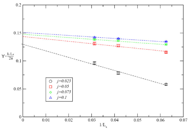
Figure 10.8: $\Upsilon$ as a function of $1/L_{s}$ for $L_{t}=56$ ($\mu=0.8$ and $L_{s}=32$).

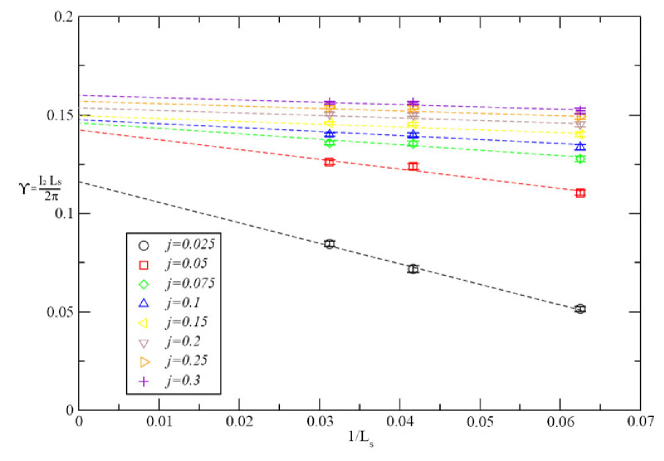
Figure 10.9: $\Upsilon$ as a function of $1/L_{s}$ for $L_{t}=48$ ($\mu=0.8$ and $L_{s}=32$).

10.2.2 Critical Temperature Range

In a conservative conclusion, the only phase range we can be sure about is that above $L_{t}=56$ and the one below $L_{t}=4$. For $L_{t}\geq 56$ infinite volume extrapolations lead to a perfect straight line, and a non-zero value of $\Upsilon$, implying superfluidity. For $L_{t}\leq 4$, even without extrapolation, the curves are parabolic, Fig.10.1, thus, they could be associated with the non-superfluid state ($\Upsilon=0$). This then leaves us with an uncertain range from $L_{t}=6-54$, which is huge! However, as I stated before this is a conservative conclusion. As we deduced through the plot of $\Upsilon$ against $L_{t}$ for $j=0.025$ (Fig. 10.3) the critical point could plausibly occur at $L_{t}\sim 6$, in which case all extrapolations above this point would be of the type $\Upsilon(j)\propto\Upsilon(0)+Aj$. This could very well be the case for $1/T$ above $L_{t}=24$, even though we can’t explain the dips at low $j$. This then leaves us with the range $L_{t}=6-22$ as the uncertain domain, due to the fact that these curves follow a "s" shape which could be either a linear or parabolic extrapolation.

Chapter 11 Summary

In Chapter 9 the calculation of baryon charge density ($n_{B}$) was extended to the conserved baryon 3-current $I_{\mu}$, where $n_{B}$ was the timelike component, $I_{0}$, of the current. Then, to force a current flow we implemented a twisted diquark source i.e. a periodically varying source, spanning the whole system.

We then investigated the current’s behaviour with a change of density $\mu$, for two temperatures: $\frac{\Upsilon_{0}}{T}=0.565(1)$ and $\frac{\Upsilon_{0}}{T}=9.043(1)$, corresponding to lattice lengths $L_{t}=4$ and $L_{t}=64$ respectively. We found that a superfluid phase does exist at high density ($\mu=0.8$) and low temperature $\frac{\Upsilon_{0}}{T}=9.043(1)$; but for high temperature, $\frac{\Upsilon_{0}}{T}=0.565(1)$, the current is always zero, Figs. 9.6 and 9.7. For the low temperature case we found that the current density has a phase transition in the region $0.65<\mu_{c}<0.68$, Fig. 9.6. This transition region corresponds to that of chiral symmetry restoration in [12].

These findings show that the low temperature, high density, phase of the 2+1d NJL model is a thin film superfluid, and the transition from this superfluid phase at high density to a non-superfluid phase at low density is of 1st order.

Initially results were presented in a spatially dependent form, so according to the size of lattice used different results were obtained for the current. We later showed that it is better to work with the spatially independent helicity modulus, $\Upsilon$, defined as the constant of proportionality $I_{2}=\Upsilon 2\pi/L_{2}$. The non-zero value of the helicity modulus was then determined in the thermodynamic limit for low temperature ($\frac{\Upsilon_{0}}{T}=9.043(1)$) and high chemical potential ($\mu=0.8$) as $\Upsilon=0.1413(14)$ . We also showed that this falls to $\sim 0$ at higher temperatures ($\frac{\Upsilon_{0}}{T}=0.565(1))$. Therefore, the ratio $\Upsilon/\Sigma$ that represents the superfluid phase of the $2+1d$ NJL model at high density is given as $\frac{\Upsilon}{0.71}=0.199(1)\sim 0.2$

Once we had found the presence of a superfluid phase, next, we wanted to test whether this superfluid behaviour was due to the binding and unbinding of vortices, as described by the KT theory for 2-dimensional critical systems. In Chapter 10 we started by calculating the critical temperature predicted by the KT theory. Using our value of $\Upsilon$ this critical temperature was found to be $\frac{\Upsilon_{0}}{T}=0.637\sim\frac{2}{\pi}$, which implies a lattice length $L_{t}=4.51(44)$.

We then showed that by plotting $\Upsilon$ against $L_{t}$ for low $j$ ($j=0.025$ in our case), we obtained a very good straight line fit that intersects the $L_{t}$ axis at a point near the KT critical length prediction, Fig. 10.4 and 10.5. Through a straight line extrapolation ($\Upsilon\propto AL_{t}+B$) this critical point was found to be at $L_{t}\sim 6(2)$. This point corresponds to the KT prediction within error. Also, this critical transition point seems to be of $2nd$ order. However, in order to make any conclusive statements about the critical point, further study is still needed, maybe using larger volumes, $L_{s}>32$, and smaller diquark source values, $j<0.025$.

We also showed that at low temperature, $\frac{\Upsilon_{0}}{T}\geq 7.9$ (or in terms of lattice size $L_{t}\geq 56$), the dip of $\Upsilon$ at low $j$ can be put down to finite volume effects, which disappears when we extrapolate to the infinite volume limit. However, even though the plots between $L_{t}=24-54$ do follow straight lines for high $j$, similar infinite volume extrapolations do not eliminate the dips at low $j$. The domain between $L_{t}=6-22$ is even more puzzling. In this area we cannot easily apply a straight line extrapolation, as the curves of $\Upsilon$ against $j$ are parabolic at low $j$.

So, in order to construct a conclusive phase diagram for $\Upsilon$ against $L_{t}$, we not only need to confirm the location of the critical point, but we also need to investigate and explain the strange behaviour of $\Upsilon$ in the intermediate temperature range.

Appendix A Schwarzschild Spacetime

The ’Schwarzschild geometry’ describes a spherically symmetric spacetime outside a star, and its properties are determined by one parameter, the mass M. The Schwarzschild metric, in spherical polar coordinates, takes the form:

$$g_{\mu\nu}=\left(\begin{array}[]{cccc}F&0&0&0\\ 0&-F^{-1}&0&0\\ 0&0&-r^{2}&0\\ 0&0&0&-r^{2}\sin(\theta)\\ \end{array}\right)$$ (A.1)

This type of spacetime geometry is said to be static, due to the fact that (i) all metric components are independent of $t$, and (ii) the geometry is unchanged by time reversal, $t\rightarrow-t$.

A.1 Geodesic Equations

The equations of motion in Schwarzschild spacetime can be derived by using the covariant form of Newton’s second law of motion,

$$F^{\mu} = \frac{Dp^{\mu}}{D\tau}$$ (A.2)

$$= \frac{dp^{\mu}}{d\tau}+\Gamma^{\mu}_{\nu\rho}\frac{dx^{\nu}}{d\tau}p^{\rho}$$

where we have $p^{\mu}=m\frac{dx^{\mu}}{d\tau}$, and for free fall we have $F^{\mu}=0$, then the equations of motion are:

$$0=\frac{d^{2}x^{\mu}}{d\tau^{2}}+\Gamma^{\mu}_{\nu\rho}\frac{dx^{\nu}}{d\tau}\frac{dx^{\rho}}{d\tau}$$ (A.3)

Now, using this and the appropriate Christoffels we are able to determine the equations of motion. Alternatively, by using the Schwarzschild Lagrangian

$$L=\frac{1}{2}[(1-\frac{2M}{r})\dot{dt}^{2}-(1-\frac{2M}{r})^{-1}\dot{dr}^{2}-r^{2}\dot{d\theta}^{2}-(r^{2}\sin^{2}\theta)\dot{d\phi}^{2}]$$ (A.4)

we find

$$\frac{\partial L}{\partial t} = 0\qquad\frac{\partial L}{\partial\dot{t}}=(1-\frac{2M}{r})\dot{t}$$

$$\frac{d}{d\lambda}\frac{\partial L}{\partial\dot{t}} = (1-\frac{2M}{r})\ddot{t}+\frac{2M}{r^{2}}\dot{r}\dot{t}$$

$$\frac{\partial L}{\partial r} = \frac{M}{r^{2}}\dot{t}^{2}+\frac{M}{r}^{2}(1-\frac{2M}{r})^{-2}\dot{r}^{2}-r\dot{\theta}^{2}-r\dot{\phi}^{2}\sin^{2}\theta$$

$$\frac{\partial L}{\partial\dot{r}} = -(1-\frac{2M}{r})^{-1}\dot{r}$$

$$\frac{d}{d\lambda}\frac{\partial L}{\partial\dot{r}} = -(1-\frac{2M}{r})^{-1}\ddot{r}+\frac{2M}{r^{2}}(1-\frac{2M}{r})^{-2}\dot{r}\dot{r}$$

$$\frac{\partial L}{\partial\theta} = -r^{2}\sin\theta\cos\theta\dot{\phi}^{2}\qquad\frac{\partial L}{\partial\dot{\theta}}=-r^{2}\dot{\theta}$$

$$\frac{d}{d\lambda}\frac{\partial L}{\partial\dot{\theta}} = -2r\dot{r}\dot{\theta}-r^{2}\ddot{\theta}$$

$$\frac{\partial L}{\partial\phi} = 0\qquad\frac{\partial L}{\partial\dot{\phi}}=-r^{2}\sin^{2}\theta\dot{\phi}^{2}$$

$$\frac{d}{d\lambda}\frac{\partial L}{\partial\dot{\phi}} = -2r\dot{r}\sin^{2}\theta\dot{\phi}-2r^{2}\sin\theta\cos\theta\dot{\phi}-r^{2}\sin^{2}\theta\ddot{\phi}$$

and substituting into the Euler equation

$$\frac{\partial L}{\partial x^{\mu}}-\frac{d}{d\lambda}\frac{\partial L}{\partial\dot{x}^{\mu}}=0$$ (A.9)

we have the equations of motion for Schwarzschild spacetime

$$0 = (1-\frac{2M}{r})\ddot{t}+\frac{2M}{r^{2}}\dot{r}\dot{t}=0$$ (A.10)

$$0 = \frac{M}{r^{2}}\dot{t}^{2}-r\dot{\theta}^{2}-r\dot{\phi}^{2}\sin^{2}\theta+(1-\frac{2M}{r})^{-1}\ddot{r}$$ (A.11)

$$- \frac{M}{r^{2}}(1-\frac{2M}{r})^{-2}\dot{r}^{2}$$

$$0 = -r^{2}\sin\theta\cos\theta\dot{\phi}^{2}+2r\dot{r}\dot{\theta}+r^{2}\ddot{\theta}$$ (A.12)

$$0 = 2r\dot{r}\sin^{2}\theta\dot{\phi}+2r^{2}\sin\theta\cos\theta\dot{\phi}+r^{2}\sin^{2}\theta\ddot{\phi}$$ (A.13)

A.2 Riemann Components in the Orthonormal Frame

The spacetime line interval, Eqn. (1.11), can be rewritten using tetrad transformations (discussed in the next section):

$$\omega^{t}=(1-\frac{2M}{r})^{\frac{1}{2}}dt\qquad\omega^{r}=(1-\frac{2M}{r})^{-\frac{1}{2}}dr\qquad\omega^{\theta}=rd\theta\qquad\omega^{\phi}=r\sin(\theta)d\phi$$ (A.14)

as

$$ds^{2}=(\omega^{t})^{2}-(\omega^{r})^{2}-(\omega^{\theta})^{2}-(\omega^{\phi})^{2}$$ (A.15)

This now has the Minkowski metric

$$g_{\mu\nu}=\left(\begin{array}[]{cccc}1&0&0&0\\ 0&-1&0&0\\ 0&0&-1&0\\ 0&0&0&-1\\ \end{array}\right)$$ (A.16)

Noting that the metric can be written as:

$$dg_{\mu\nu}=\omega_{\mu\nu}+\omega_{\nu\mu}$$ (A.17)

and using the fact that:

$$dg_{\mu\nu}=\frac{\partial g_{\mu\nu}}{\partial x^{\alpha}}dx^{\alpha}=0$$ (A.18)

we then have[2]:

$$\omega_{\mu\nu}=-\omega_{\nu\mu}$$ (A.19)

which implies $\omega$ is antisymmetric, i.e. it has only six unique components and $\omega_{\mu\nu}=0$ for $\mu=\nu$; and we have the conditions:

$$\omega^{0}_{i}=\omega^{i}_{0}\qquad\omega^{i}_{j}=-\omega^{j}_{i}$$ (A.20)

We can now write the exterior derivatives of $\omega^{\mu}$

$$d\omega^{t} = \frac{1}{2}(1-\frac{2M}{r})^{-\frac{1}{2}}(\frac{2M}{r^{2}})dr\wedge dt$$ (A.21)

$$= \frac{M}{r^{2}}(1-\frac{2M}{r})^{-\frac{1}{2}}\omega^{r}\wedge\omega^{t}$$

$$d\omega^{r} = 0$$ (A.22)

$$d\omega^{\theta} = dr\wedge d\theta=\frac{1}{r}(1-\frac{2M}{r})^{\frac{1}{2}}\omega^{r}\wedge\omega^{\theta}$$ (A.23)

$$d\omega^{\phi} = \sin(\theta)dr\wedge d\phi+r\cos(\phi)d\theta\wedge d\phi$$ (A.24)

$$= \frac{1}{r}(1-\frac{2M}{r})^{\frac{1}{2}}\omega^{r}\wedge\omega^{\phi}+\frac{\cot(\theta)}{r}\omega^{\theta}\wedge\omega^{\phi}$$

Now, using Cartan’s equation

$$d\omega^{\mu}=\omega^{\alpha}\wedge\omega^{\mu}_{\alpha}+\Omega^{\mu}$$ (A.25)

with zero torsion $(\Omega^{\mu}=0)$, we can write

$$d\omega^{t} = \omega^{r}\wedge\omega^{t}_{r}+\omega^{\theta}\wedge\omega^{t}_{\theta}+\omega^{\phi}\wedge\omega^{t}_{\phi}$$ (A.26)

$$d\omega^{r} = \omega^{t}\wedge\omega^{r}_{t}+\omega^{\theta}\wedge\omega^{r}_{\theta}+\omega^{\phi}\wedge\omega^{r}_{\phi}$$ (A.27)

$$d\omega^{\theta} = \omega^{t}\wedge\omega^{\theta}_{t}+\omega^{r}\wedge\omega^{\theta}_{r}+\omega^{\phi}\wedge\omega^{\theta}_{\phi}$$ (A.28)

$$d\omega^{\phi} = \omega^{t}\wedge\omega^{\phi}_{t}+\omega^{r}\wedge\omega^{\phi}_{r}+\omega^{\theta}\wedge\omega^{\phi}_{\theta}$$ (A.29)

Comparing Eqns. (A.21)-(A.24) with Eqns. (A.26)-(A.29) we find the six unique components of $\omega^{\mu}_{\nu}$ as

$$\omega^{t}_{r} = \frac{M}{r^{2}}(1-\frac{2M}{r})^{-\frac{1}{2}}\omega^{t}=\frac{M}{r^{2}}dt=\omega^{r}_{t}$$ (A.30)

$$\omega^{\theta}_{r} = \frac{1}{r}(1-\frac{2M}{r})^{\frac{1}{2}}\omega^{\theta}=(1-\frac{2M}{r})^{\frac{1}{2}}d\theta=-\omega^{r}_{\theta}$$ (A.31)

$$\omega^{\phi}_{r} = \frac{1}{r}(1-\frac{2M}{r})^{\frac{1}{2}}\omega^{\phi}=\sin(\theta)(1-\frac{2M}{r})^{\frac{1}{2}}d\phi=-\omega^{r}_{\phi}$$ (A.32)

$$\omega^{\phi}_{\theta} = \frac{\cot(\theta)}{r}\omega^{\phi}=\cos(\theta)d\phi=-\omega^{\theta}_{\phi}$$ (A.33)

$$\omega^{\theta}_{t} = \omega^{t}_{\theta}=0$$ (A.34)

$$\omega^{\phi}_{t} = \omega^{t}_{\phi}=0$$ (A.35)

Now, using:

$$R^{\mu}_{\nu}=d\omega^{\mu}_{\nu}+\omega^{\mu}_{\alpha}\wedge\omega^{\alpha}_{\nu}$$ (A.36)

we can write the six independent components of the Riemann tensor:

$$R^{t}_{r} = d\omega^{t}_{r}+\omega^{t}_{\alpha}\wedge\omega^{\alpha}_{r}=d\omega^{t}_{r}+\omega^{t}_{\theta}\wedge\omega^{\theta}_{r}+\omega^{t}_{\phi}\wedge\omega^{\phi}_{r}$$

$$= -\frac{2M}{r^{3}}dr\wedge dt=-\frac{2M}{r^{3}}\omega^{r}\wedge\omega^{t}$$

$$\Rightarrow R^{t}_{rrt}=R_{trrt}=-\frac{2M}{r^{3}}$$

$$R^{\theta}_{r} = d\omega^{\theta}_{r}+\omega^{\theta}_{\alpha}\wedge\omega^{\alpha}_{r}=d\omega^{\theta}_{r}+\omega^{\theta}_{t}\wedge\omega^{t}_{r}+\omega^{\theta}_{\phi}\wedge\omega^{\phi}_{r}$$

$$= \frac{1}{2}(1-\frac{2M}{r})^{-\frac{1}{2}}\frac{2M}{r^{2}}dr\wedge d\theta=\frac{M}{r^{3}}\omega^{r}\wedge\omega^{\theta}$$

$$\Rightarrow R^{\theta}_{rr\theta}=-R_{\theta rr\theta}=\frac{M}{r^{3}}$$

$$R^{\phi}_{r} = d\omega^{\phi}_{r}+\omega^{\phi}_{\alpha}\wedge\omega^{\alpha}_{r}=d\omega^{\phi}_{r}+\omega^{\phi}_{t}\wedge\omega^{t}_{r}+\omega^{\phi}_{\theta}\wedge\omega^{\theta}_{r}$$

$$= \cos(\theta)(1-\frac{2M}{r})^{\frac{1}{2}}d\theta\wedge d\phi+\sin(\theta)\frac{M}{r^{2}}(1-\frac{2M}{r})^{-\frac{1}{2}}dr\wedge d\phi$$

$$+ \cos(\theta)(1-\frac{2M}{r})^{1}{2}d\phi\wedge d\theta$$

$$= \frac{\cot(\theta)}{r^{2}}(1-\frac{2M}{r})^{\frac{1}{2}}\omega^{\theta}\wedge\omega^{\phi}+\frac{M}{r^{3}}\omega^{r}\wedge\omega^{\phi}$$

$$+ \frac{\cot(\theta)}{r^{2}}(1-\frac{2M}{r})^{\frac{1}{2}}\omega^{\phi}\wedge\omega^{\theta}=\frac{M}{r^{3}}\omega^{r}\wedge\omega^{\phi}$$

$$\Rightarrow R^{\phi}_{rr\phi}=-R_{\phi rr\phi}=\frac{M}{r^{3}}$$

$$R^{\phi}_{\theta} = d\omega^{\phi}_{\theta}+\omega^{\phi}_{\alpha}\wedge\omega^{\alpha}_{\theta}=d\omega^{\phi}_{\theta}+\omega^{\phi}_{t}\wedge\omega^{t}_{\theta}+\omega^{\phi}_{r}\wedge\omega^{r}_{\theta}$$

$$= -\sin(\theta)d\theta\wedge d\phi-\sin(\theta)(1-\frac{2M}{r})d\phi\wedge d\theta$$

$$= -\frac{1}{r^{2}}\omega^{\theta}\wedge\omega^{\phi}+\frac{1}{r^{2}}(1-\frac{2M}{r})\omega^{\theta}\wedge\omega^{\phi}=-\frac{2M}{r^{3}}\omega^{\theta}\wedge\omega^{\phi}$$

$$\Rightarrow R^{\phi}_{\theta\theta\phi}=-R_{\phi\theta\theta\phi}=-\frac{2M}{r^{3}}$$

$$R^{\theta}_{t} = d\omega^{\theta}_{t}+\omega^{\theta}_{\alpha}\wedge\omega^{\alpha}_{t}=d\omega^{\theta}_{t}+\omega^{\theta}_{r}\wedge\omega^{r}_{t}+\omega^{\theta}_{\phi}\wedge\omega^{\phi}_{t}$$

$$= \frac{M}{r^{2}}(1-\frac{2M}{r})^{\frac{1}{2}}d\theta\wedge dt=\frac{M}{r^{3}}\omega^{\theta}\wedge\omega^{t}$$

$$\Rightarrow R^{\theta}_{t\theta t}=-R_{\theta t\theta t}=\frac{M}{r^{3}}$$

$$R^{\phi}_{t} = d\omega^{\phi}_{t}+\omega^{\phi}_{\alpha}\wedge\omega^{\alpha}_{t}=d\omega^{\phi}_{t}+\omega^{\phi}_{r}\wedge\omega^{r}_{t}+\omega^{\phi}_{\theta}\wedge\omega^{\theta}_{t}$$

$$= \frac{M}{r^{2}}(1-\frac{2M}{r})^{\frac{1}{2}}\sin(\theta)d\theta\wedge dt=\frac{M}{r^{3}}\omega^{\phi}\wedge\omega^{t}$$

$$\Rightarrow R^{\phi}_{t\phi t}=-R_{\phi t\phi t}=\frac{M}{r^{3}}$$

A.3 Tetrad Transformation

In Eqn. (A.14) we transformed from the coordinate frame to an orthonormal frame. This is achieved by using the tetrad of the form:

$$e^{a}_{\mu}=\left(\begin{array}[]{cccc}F^{\frac{1}{2}}&0&0&0\\ 0&F^{-\frac{1}{2}}&0&0\\ 0&0&r&0\\ 0&0&0&r\sin(\theta)\\ \end{array}\right)$$ (A.43)

This takes a 4-vector, given in the coordinate frame, and maps it to the equivalent in the orthonormal frame. We can then determine the inverse tetrad, i.e. a tetrad that takes vectors in the orthonormal frame and maps them to the coordinate frame. We find this by using the inverse of (A.43),

$$(e^{-1})^{\mu}_{a}=\left(\begin{array}[]{cccc}F^{-\frac{1}{2}}&0&0&0\\ 0&F^{\frac{1}{2}}&0&0\\ 0&0&\frac{1}{r}&0\\ 0&0&0&\frac{1}{r\sin(\theta)}\\ \end{array}\right),$$ (A.44)

which has the property:

$$e^{a}_{\mu}(e^{-1})^{\mu}_{b}=\delta^{a}_{b}$$ (A.45)

Therefore, (A.44) takes vectors in the orthonormal frame and maps them to the coordinate frame.

A.4 Riemann Components in the Coordinate Frame

In Sec. A.2 the unique components of the Riemann tensor were calculated in the orthonormal frame. In order to determine the components in the coordinate basis we will use the transformation tetrad given in Eqn. A.44. Before we can us the tetrad, (A.44), we need to adjust it so it is able to take covectors in the orthonormal frame, rather than vectors:

$$(e^{-1})^{\mu}_{a}g_{\mu\nu}\eta^{ab}=(e^{-1})_{\nu}^{b}=\left(\begin{array}[]{cccc}F^{\frac{1}{2}}&0&0&0\\ 0&F^{-\frac{1}{2}}&0&0\\ 0&0&r&0\\ 0&0&0&r\\ \end{array}\right),$$ (A.46)

which is just Eqn. (A.43). Then using this we have:

$$\Rightarrow\qquad A_{\mu}(\textrm{coordinate frame})=(e^{-1})_{\mu}^{a}A_{a}(\textrm{orthonormal frame})$$

Now using this tetrad we can transform the orthonormal Riemann tensor components as:

$$R_{\mu\nu\alpha\beta}=(e^{-1})_{\mu}^{a}(e^{-1})_{\nu}^{b}(e^{-1})_{\alpha}^{c}(e^{-1})_{\beta}^{d}R_{abcd}$$

Now using the components given in Sec. A.2 we have:

$$R^{\prime}_{trrt} = (e^{-1})_{t}^{t}(e^{-1})_{r}^{r}(e^{-1})_{r}^{r}(e^{-1})_{t}^{t}R_{trrt}=F^{\frac{1}{2}}F^{-\frac{1}{2}}F^{-\frac{1}{2}}F^{\frac{1}{2}}(-\frac{2M}{r^{3}})=-\frac{2M}{r^{3}}$$

$$R^{\prime}_{\theta rr\theta} = (e^{-1})_{\theta}^{\theta}(e^{-1})_{r}^{r}(e^{-1})_{r}^{r}(e^{-1})_{\theta}^{\theta}R_{\theta rr\theta}=rF^{-\frac{1}{2}}F^{-\frac{1}{2}}r(-\frac{M}{r^{3}})=-\frac{MF^{-1}}{r}$$

$$R^{\prime}_{\phi rr\phi} = (e^{-1})_{\phi}^{\phi}(e^{-1})_{r}^{r}(e^{-1})_{r}^{r}(e^{-1})_{\phi}^{\phi}R_{\phi rr\phi}=rF^{-\frac{1}{2}}F^{-\frac{1}{2}}r(-\frac{M}{r^{3}})=-\frac{MF^{-1}}{r}$$

$$R^{\prime}_{\phi\theta\theta\phi} = (e^{-1})_{\phi}^{\phi}(e^{-1})_{\theta}^{\theta}(e^{-1})_{\theta}^{\theta}(e^{-1})_{\phi}^{\phi}R_{\phi\theta\theta\phi}=rrrr(\frac{2M}{r^{3}})=2Mr$$

$$R^{\prime}_{\theta t\theta t} = (e^{-1})_{\theta}^{\theta}(e^{-1})_{t}^{t}(e^{-1})_{\theta}^{\theta}(e^{-1})_{t}^{t}R_{\theta t\theta t}=rF^{\frac{1}{2}}rF^{\frac{1}{2}}(-\frac{M}{r^{3}})=-\frac{MF}{r}$$

$$R^{\prime}_{\phi t\phi t} = (e^{-1})_{\phi}^{\phi}(e^{-1})_{t}^{t}(e^{-1})_{\phi}^{\phi}(e^{-1})_{t}^{t}R_{\phi t\phi}t=rF^{\frac{1}{2}}rF^{\frac{1}{2}}(-\frac{M}{r^{3}})=-\frac{MF}{r}$$

Therefore, the Riemann tensor components in the coordinate frame are given as:

$$R^{\prime}_{trrt} = -\frac{2M}{r^{3}}\qquad R^{\prime}_{\theta rr\theta}=-\frac{MF^{-1}}{r}\qquad R^{\prime}_{\phi rr\phi}=-\frac{MF^{-1}}{r}$$

$$R^{\prime}_{\phi\theta\theta\phi} = 2Mr\qquad R^{\prime}_{\theta t\theta t}=-\frac{MF}{r}\qquad R^{\prime}_{\phi t\phi t}=-\frac{MF}{r}$$

Appendix B XY Model and the KT Transition

B.1 Spin Systems

B.1.1 The Ising Model

The most basic spin system is the Ising model, which is generally used to describe magnetisation. It consists of $N$ spin sites, each taking a value of $+1$ or $-1$ (i.e. up and down respectively). In its simplest form it describes a 1-dimensional lattice, usually with the $N$ sites in a chain formation and periodic boundaries. Other simplifications include a uniform external field at each site, $H_{i}=H$, so that the only interaction between spins is that between the nearest neighbours, symbolised by $J$. This system is then described by the Hamiltonian:

$$-\mathcal{H}=\sum_{i=1}^{N}H_{i}S_{i}+J\sum_{<i,j>}S_{i}S_{j}$$ (B.1)

The partition function of this model is then written as:

$$Z=\sum_{[S_{i}]}\exp(-\beta\mathcal{H}(S_{i}))$$ (B.2)

where $\beta=1/(k_{B}T)$, and the the sum is taken over all possible states i.e. a total of $2^{N}$ possible spin states. Then, to extract thermodynamic information from the partition function we define the free energy of the Ising model as,

$$F=-k_{B}T\ln Z$$

From this we can determine the magnetisation of the system,

$$M=\frac{1}{N}<S>\qquad<S>=\sum_{i=1}^{N}<S_{i}>=-\sum_{i=1}^{N}\frac{\partial F}{\partial H_{i}}$$

where $<S_{i}>$ is the average spin of the $i^{th}$ site. The correlation function, a measure of the influence exerted by a given spin $S_{i}$ on other spin sites $S_{j}$, is given as:

$$G_{ij}=<S_{i}S_{j}>-<S_{i}><S_{j}>;$$

Since the interaction between spins favours alignment, a nearby spin $S_{j}$ will tend to assume the same orientation as $S_{i}$; however thermal fluctuations counteract this tendency and exert a de-correlating effect. Thus we expect some correlation that weakens as the distance between $S_{i}$ and $S_{j}$ increases, also at a fixed distance apart the correlation will be stronger when the temperature is lower, see Fig. B.1 [27].

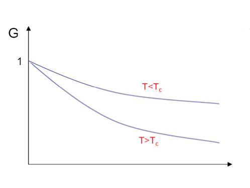
Figure B.1: Ratio of the correlation function $G=G(r_{ij})/G(0)$, for two different temperatures $T$ (not to scale).

So, when the temperature is low we can assume that the majority of spin states are correlated, which in the absence of an external field leads to the phenomenon of spontaneous magnetization, $M_{s}$. For the 1-dimensional Ising model this does not occur for $T\neq 0$, but there is a trivial phase change at $T=0$, i.e. when the thermal energy is zero all the spins are aligned. However, in 2-dimensions there is a second order phase transition at the Curie temperature $T=T_{c}$ [27][28], Fig. B.2.

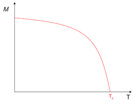
Figure B.2: Spontaneous magnetization in 2-dimensions against temperature.

B.1.2 The XY Model

The restriction of the Ising model is that the spin vector can only assume one of 2 discrete values. Even though for some cases this is fine, a more realistic model is the XY model. In this case spin is a continuous vector in a plane (for 2 dimensions). This model is characterized by the Hamiltonian:

$$-\mathcal{H}=\sum_{i=1}^{N}H_{i}S^{z}_{i}+J\sum_{<i,j>}\vec{S}_{i}\cdot\vec{S}_{j}$$ (B.3)

where the spins are classical vectors of unit length aligned in the plane. For zero external field we can write:

$$-\mathcal{H}=J\sum_{<i,j>}\vec{S}_{i}\cdot\vec{S}_{j}=J\sum_{<i,j>}\cos(\Phi_{i}-\Phi_{j}),$$ (B.4)

where $\Phi$ is the angle between the spin direction and an arbitrarily chosen axis, and is a continuous variable.

In this 2-dimensional model, spin excitations (spin waves) are easier to excite thermally than for the Ising model, they are so strong that they can destroy long-range order at any finite T; so, in the case of 2-dimensions, symmetry breaking for $T\geq 0$ does not occur (Mermin-Wagner theorem [29]). On the other hand, in 1973, Kosterlitz and Thouless showed that a kind of phase transition can exist for the $2d$ XY model, or more accurately there is a critical point at non-zero temperature. It arises not from the long-range ordering like spontaneous magnetization but from the excitations of vortex-antivortex pairs [31][32].

B.2 Phase Transitions in the XY Model

B.2.1 The Critical Phase in the XY Model

Vortices

If we consider small spin variations,$\Phi_{i}-\Phi_{j}\ll 1$, then we can expand B.4 as:

$$\mathcal{H}\simeq E_{0}+\frac{1}{2}J\sum_{<i,j>}(\Phi_{i}-\Phi_{j})^{2}=\frac{Ja^{2}}{2}\sum_{i}|\vec{\nabla}\Phi(i)|^{2}$$ (B.5)

where $a$ is the lattice spacing. This can now be taken to the continuum limit, so that $\Phi(r)$ becomes a scalar field, and the sum becomes an integral over the $2d$ area:

$$\mathcal{H}-E_{0}=\frac{J}{2}\int d^{2}r|\vec{\nabla}\Phi(r)|^{2}$$ (B.6)

In this $2d$ state of continuous spin states a possible excitation above the (perfectly ordered) ground state is a vortex, Fig. B.3. Any line integral along a closed path around the center of the vortex will give:

$$\oint\vec{\nabla}\Phi(\vec{r})\cdot d\vec{r}=2\pi q\qquad\Rightarrow\qquad\begin{array}[]{c}\Phi=q\phi\\ |\vec{\nabla}\Phi(r)|=\frac{q}{r}\end{array}$$ (B.7)

where $q$ is the vorticity and $\phi$ is the angle to $\vec{r}$.

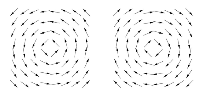
Figure B.3: Vortex with vorticity $|q|=1$

Now using (B.6) and (B.7) we can find the energy of this vortex above the ground state energy:

$$E=\int_{a}^{R}2\pi rdr\frac{J}{2}(\frac{q}{r})^{2}=\pi J\ln(\frac{R}{a})q^{2}$$ (B.8)

here, $R$ is the size of the system [33][27], and $a$ is the lower cut off (as the theory diverges as $r\rightarrow 0$). Now it can be seen that the energy of the vortex increases logarithmically with the size of the system.

Thermodynamics of Single Vortices

A vortex can be put onto any lattice site, thus the number of configurations is $(R/a)^{2}$, and then we can write the entropy of the vortex as

$$S=2k_{B}\ln(\frac{R}{a})$$ (B.9)

Therefore, the free energy, $F=E-TS$, is positive and large at low temperatures. Thus, it is not very easy to thermally excite single vortices at low temperature. But, as temperature increases, the free energy decreases, and at a critical temperature $T_{KT}$ the free energy vanishes:

$$k_{B}T_{KT}=\frac{\pi J}{2}$$ (B.10)

Then, above $T_{KT}$ a large number of vortices are thermally excited.

Vortex-Antivortex "Dipole" Pairs

Even though it is difficult to excite single vortices at low temperature, it does not mean none exist. In the low temperature phase it becomes more favorable to excite pairs of vortices, i.e. a vortex-antivortex pair. To see this we start by writing the energy of a system of two vortices, with vorticity $q_{1}$ and $q_{2}$:

$$\Phi = \Phi_{1}(\vec{r}_{1})\Phi_{2}(\vec{r}_{2})$$

$$E(q_{1},q_{2}) = -\pi J(q_{1}+q_{2})^{2}\ln(\frac{R}{a})$$ (B.11)

$$- 2\pi Jq_{1}q_{2}\ln(\frac{|\vec{r}_{1}-\vec{r}_{2}|}{a})$$

where for a vortex and antivortex pair $q_{1}=-q_{2}$, thus we have:

$$E(q_{1},q_{2})=2\pi Jq^{2}\ln(\frac{|\vec{r}_{1}-\vec{r}_{2}|}{a})$$ (B.12)

From this you can see that the self-energy of a vortex-antivortex pair is small when the vortices are close together. Thus, as the energy of a "dipole" pair is smaller than a single vortex, it is easier to excite a pair of opposite vortices than a single vortex.

Critical Phase of the XY Model

We can now see that at low temperature, $0<T<T_{KT}$, there will be a finite density of low energy vortex-antivortex pairs, of zero total vorticity. Then, at high temperatures, $T>T_{KT}$, there will be a large concentration of unbound vortices.

In this picture the critical temperature is then associated with the unbinding of vortex-antivortex pairs; the pairs are bound strongly to each other at low temperature, and as the temperature increases, the number of pairs increases. Then, at the critical temperature $T_{KT}$, vortex-antivortex pairs start to separate and become free; this is called the KT (Kosterlitz and Thouless) phase transition.

Correlation Length of Vortex Pairs

Due to the $KT$ transition the correlation function of the XY model changes behaviour as it crosses the critical point $T_{KT}$. Above the critical point, when the vortices are unbound and free to interact with each other, the correlation function behaves in a classic way:

$$<S_{i}S_{j}>=e^{-\frac{r}{\xi}},$$ (B.13)

with the correlation length:

$$\xi=\frac{a}{\ln T/J}$$ (B.14)

However, below the critical temperature the correlation function shifts to a power-law:

$$<S_{i}S_{j}>=(\frac{a}{r})^{\frac{1}{\xi}}$$ (B.15)

and the critical exponent becomes:

$$\frac{1}{\xi}=\frac{T}{2\pi J}$$ (B.16)

This can be understood in the following way: at low temperature vortices bind into dipole pairs, whose influence on the system is confined to small distances, thus the only important large distance interactions are spin waves. This phase is then described by the power-law behaviour of the correlation function. As the temperature rises the size of the dipole pairs increases, and diverges at $T=T_{KT}$ when free vortices appear. These free vortices then interact, and in the process, the low temperature dominance of spin waves is destroyed. This phase is then described by an exponential behaviour of the correlation function.

B.3 The KT Transition and Superfluidity in $2d$

One application of the KT transition, i.e the binding and unbinding of vortices at the critical temperature $T_{KT}$, is in understanding superfluidity in thin films. For $d>2$ Bose-Einstein condensation occurs in a Bose gas at low temperature, and this condensed phase is defined by the breaking of a $U(1)$ global gauge symmetry. However, for systems with $d\leq 2$ the breaking of a $U(1)$ global gauge symmetry is prohibited by the Mermin-Wagner theorem, i.e. no phase transition to a state with long-range order can occur at finite temperatures. On the other hand, topological phase transitions are possible; and the binding and unbinding of vortices in two dimensions leads to a type of phase transition.

B.3.1 Superfluids and the XY model

Our previous calculations, relating to vortices in the XY model can be directly applied to the study of superfluids. For single vortices, the XY spin angle $\Phi$ (B.5) can be related to the phase of a particle’s wave function in the superfluid condensate state:

$$\Psi=\sqrt{n_{0}}\exp(-i\Phi(t,\vec{r}))$$ (B.17)

where $n_{0}$ is the number of condensate particles (superfluid density). Then the current density of the superfluid is given by:

$$I_{cond} = \frac{i\hbar}{2m}(\Psi\vec{\nabla}\Psi^{*}-\Psi^{*}\vec{\nabla}\Psi)$$ (B.18)

$$= \frac{\hbar}{m}n_{0}\vec{\nabla}\Phi$$

$$= \Upsilon\vec{\nabla}\Phi\qquad\rightarrow\qquad\Upsilon=\frac{\hbar}{m}n_{0}$$

where $m$ is the mass of the superfluid particle; and $\Upsilon$ is the constant of proportionality between the current density and the phase angle, and is known as the helicity modulus ($\Upsilon$). The phase angle $\Phi$ can be associated with the spin angle as in the XY-model or with a particles phase as in the superfluid condensate.

If we divide both sides of (B.18) by the density $n_{0}$, we have the velocity of the condensate particles:

$$\vec{v}_{cond}(\vec{r})=\frac{\hbar}{m}\vec{\nabla}\Phi$$ (B.19)

This can now be inserted into the energy of a superfluid velocity fluctuation,

$$\mathcal{H}=\frac{1}{2}mn_{0}\int d^{2}r|\vec{v}_{cond}(\vec{r})|^{2}$$ (B.20)

where $mn_{0}$ is the mass density of the superfluid. This then gives us:

$$\mathcal{=}\frac{\hbar\Upsilon}{2}\int d^{2}r(\vec{\nabla\Phi})^{2}\qquad\rightarrow\qquad\Upsilon=\frac{\hbar}{m}n_{0}$$ (B.21)

It can now be seen that this is similar to (B.6) if, as stated before, we identify the phase of the superfluid condensate with the angle of spin in the XY model and $\hbar\Upsilon=J$ . Therefore, due to this link between the XY model and superfluids, the transition from a superfluid state to a normal state for a $2d$ superfluid can be associated with the binding and unbinding of vortex pair excitations with opposite circulation. Evidence of this $KT$ behaviour is seen in superfluid Helium 4. In $3d$ there is a continuous decrease of the superfluid density with temperature, but in the 2 dimension case, for example in thin films of ${}^{4}He$, a jump in the superfluid density occurs at the critical temperature $T_{KT}$ [36].

$T_{KT}$ for Superfluids

By combining Eqns. (B.10) and (B.21) we are able to determine the critical temperature, $T_{KT}$, for superfluids:

$$\frac{1}{T_{KT}}=\frac{2}{\pi}\frac{K_{B}}{J}=\frac{2}{\pi}\frac{K_{B}}{\hbar\Upsilon}$$ (B.22)

where the final form, in terms of the helicity modulus, is the most useful form. This can be written in lattice field theory (using lattice units $K_{B}=1$, $\hbar=1$ and $L_{t}=1/T$) as:

$$L_{t}=\frac{1}{T_{KT}}=\frac{2}{\pi}\frac{1}{\Upsilon},$$ (B.23)

Appendix C Changes to QCD

C.1 Lattice QCD at $\mu\neq 0$

Lattice calculations cannot be extended to $\mu\neq 0$ due to technical problems. A quantum system, recast in Euclidean space-time, can be represented statistically in terms of the partition function:

$$\mathcal{Z}=\int dUd\bar{\psi}d\psi e^{-S[U,\bar{\psi},\psi]},$$ (C.1)

where $S=\sum_{x}\mathcal{L}_{QCD}$ is the QCD action. Then, in order to calculate this, or related expectation values,

$$<\mathcal{O}>\equiv\frac{1}{\mathcal{Z}}\int dUd\bar{\psi}d\psi\mathcal{O}e^{-S[U,\bar{\psi},\psi]},$$ (C.2)

one can explicitly integrate out the bilinear fermionic dependence leaving

$$\mathcal{Z}=\int dU\det Me^{-S_{g}[U]}$$ (C.3)

where $S_{g}$ is the gauge contribution to the action and $M=(D/\hskip 1.99997pt+m_{0})$ is the fermion kinetic matrix. Now, from the direct correspondence between Euclidean quantum field theory and statistical mechanics, it is possible to carry out the integral over gauge field configurations using Monte Carlo methods, in which the highly peaked nature of $e^{-S}$ is exploited by using it as a sampling weight. This is possible because $D/\hskip 1.99997pt$ is an anti-hermitian operator which obeys chiral symmetry, so we have $[D/\hskip 1.99997pt,\gamma_{5}]=0$ and its eigenvalues come in complex conjugate pairs, $\pm i\lambda$. Therefore, the determinant of $D/\hskip 1.99997pt$ can be written as a product of the eigenvalues, which in this case is real. Hence, we can use: $\det D/\hskip 1.99997pte^{-S_{g}}$ as the full functional weight. This is still a valid argument even with the inclusion of the chiral symmetry breaking mass term, as the eigenvalues of $D/\hskip 1.99997pt+m_{0}$ are $m_{0}\pm i\lambda$, which remain complex conjugate pairs

However, when a chemical potential is introduced we have, $M\rightarrow D/\hskip 1.99997pt+m_{0}+\mu\gamma_{0}$. As the chemical potential term is hermitian, $M$ then has complex eigenvalues, making its determinant complex; and so the importance sampling weight becomes $|\det M|e^{i\theta}e^{-S_{g}}$. This can be shown as follows:

$$\bar{\psi}M(\mu)\psi = \bar{\psi}(\gamma_{\nu}\partial_{\nu}+\mu\gamma_{0}+m)\psi$$ (C.4)

$$= \bar{\psi}\gamma_{5}\gamma_{5}(\gamma_{\nu}\partial_{\nu}+\mu\gamma_{0}+m)\psi$$

$$= \bar{\psi}\gamma_{5}(-\gamma_{\nu}\partial_{\nu}-\mu\gamma_{0}+m)\gamma_{5}\psi$$

$$= \bar{\psi}\gamma_{5}M^{{\dagger}}(-\mu)\gamma_{5}\psi$$

Therefore,

$$M(\mu) = \gamma_{5}M^{{\dagger}}(-\mu)\gamma_{5}$$

$$\Rightarrow\qquad\det M(\mu) = \det\gamma_{5}M^{{\dagger}}(-\mu)\gamma_{5}$$ (C.5)

$$= \det M^{{\dagger}}(-\mu)$$

$$= \det M^{*}(-\mu)$$

Then, for $\mu=0$, $\det M$=$\det M^{*}$ implies $\det M$ is real, but if $\mu\neq 0$, we have $\det M(\mu)$=$\det M^{*}(-\mu)$, implying $\det M$ is complex.

Therefore, the case for $\mu\neq 0$ leads to a complex phase, which in turn leads to configurations with large $e^{-S_{g}}$ cancelling and the effectiveness of the importance sampling weight becoming suppressed[15].

C.1.1 $\mu\neq 0$ in the NJL Model

In the NJL model, it can be shown that even with the introduction of a chemical potential term, the importance sampling weight remains real. Using the NJL Lagrangian, Eqn. (8.7), we have:

$$M\rightarrow\gamma_{\nu}\partial_{\nu}+\mu\gamma_{0}+m+(\sigma+i\gamma_{5}\vec{\tau}\cdot\vec{\pi})$$ (C.6)

Now, we have:

$$\bar{\psi}M(\mu)\psi= \bar{\psi} (C\gamma_{5}\otimes\tau_{2})(C^{-1}\gamma_{5}\otimes\tau_{2})(\gamma_{\nu}\partial_{\nu}+\mu\gamma_{0}+m$$

$$+ \sigma+i\gamma_{5}\vec{\tau}\cdot\vec{\pi})\psi$$

$$= \bar{\psi} (C\gamma_{5}\otimes\tau_{2})C^{-1}\gamma_{5}(\gamma_{\nu}\partial_{\nu}+\mu\gamma_{0}+m$$

$$+ \sigma-i\gamma_{5}\vec{\tau}^{*}\cdot\vec{\pi})\tau_{2}\psi$$

$$= \bar{\psi} (C\gamma_{5}\otimes\tau_{2})C^{-1}(-\gamma_{\nu}\partial_{\nu}-\mu\gamma_{0}+m$$

$$+ \sigma-i\gamma_{5}\vec{\tau}^{*}\cdot\vec{\pi})\gamma_{5}\otimes\tau_{2}\psi$$

$$= \bar{\psi} (C\gamma_{5}\otimes\tau_{2})(\gamma_{\nu}^{*}\partial_{\nu}+\mu\gamma_{0}^{*}+m$$

$$+ \sigma-i\gamma_{5}^{*}\vec{\tau}^{*}\cdot\vec{\pi})(C^{-1}\gamma_{5}\otimes\tau_{2})\psi$$

$$= \bar{\psi} (C\gamma_{5}\otimes\tau_{2})M^{*}(\mu)(C^{-1}\gamma_{5}\otimes\tau_{2})\psi$$ (C.7)

Here we have $\det M=\det M^{*}$, implying $\det M$ is real.

C.2 Staggered Fermions

The Euclidean action for a free fermion field $\psi$, in $2+1d$, is given by

$$S=\int d^{3}x\bar{\psi}(D/\hskip 1.99997pt+m_{0})\psi,$$ (C.8)

which, when discretised becomes

$$S=a^{3}\sum_{x}\left[\bar{\psi}_{x}\sum_{\nu}\left\{\gamma_{\nu}\frac{(\psi_{x+\hat{\nu}}-\psi_{x-\hat{\nu}})}{2a}\right\}+m_{0}\bar{\psi}_{x}\psi_{x}\right]$$ (C.9)

Fourier transforming this to momentum space this becomes

$$S=a^{3}\int^{\frac{\pi}{a}}_{-\frac{\pi}{a}}\frac{d^{3}p}{(2\pi)^{3}}\bar{\psi}\left[\frac{i}{a}\sum_{\nu}\gamma_{\nu}\sin(ap_{\nu})\psi+m_{0}\psi\right]$$ (C.10)

The inverse of $M$, where $S=\int\bar{\psi}M\psi$, is found to be

$$S_{F}(p)=\frac{-\frac{i}{a}\sum_{\nu}\gamma_{\nu}\sin(ap_{\nu})+m_{0}}{\frac{1}{a^{2}}\sum_{\nu}\sin^{2}(ap_{\nu})+(m_{0})^{2}}$$ (C.11)

We can see that in the case of small momentum (long wavelength) limit, the small angle approximation implies $\sin ap_{\nu}\approx ap_{\nu}$ and we recover the continuum Euclidean propagator. However, in general this represents $8$ species of fermion.

This "doubling problem" can be resolved by the staggered formulation. In this way we can reduce the number of species by a factor of $4$, which can therefore by interpreted as the physical flavours [39]. By making the transformation:

$$\psi_{x}\rightarrow\gamma^{x_{1}}_{1}\gamma^{x_{2}}_{2}\gamma^{x_{3}}_{3}\chi_{x}\qquad\bar{\psi}_{x}\rightarrow\bar{\chi}_{x}\gamma^{x_{3}}_{3}\gamma^{x_{2}}_{2}\gamma^{x_{1}}_{1}$$ (C.12)

so that $\bar{\psi}_{x}\gamma_{\nu}\psi_{x\pm\hat{\nu}}\rightarrow\eta_{\nu}(x)\bar{\chi}_{x}\chi_{x\pm\hat{\nu}}$, where $\eta_{\nu}(x)=(-1)^{x_{1}+\ldots+x_{\nu+1}}$, then the action, Eqn. (C.9), becomes:

$$S=a^{3}\sum_{x}\left[\bar{\chi}_{x}\sum_{\nu}\left\{\eta_{\nu}(x)\frac{(\chi_{x+\hat{\nu}}-\chi_{x-\hat{\nu}})}{2a}\right\}+m_{0}\bar{\chi}_{x}\chi_{x}\right]$$ (C.13)

Now, $M$ is in a reducible diagonal form, so disregarding all but one component of $\nu$, we are left with the reduced number of $2$ quark species.

Appendix D Hybrid Molecular Dynamics Code

For the 2+1d Euclidean NJL model (in the Gor’kov basis), expectation values of an observable $O$ as a function of the bosonic field configuration $[\Phi]$ are given by:

$$\langle O\rangle\equiv\mathcal{Z}^{-1}\int\mathcal{D}\Phi\mathcal{D}\Phi^{{\dagger}}O[\Phi]\sqrt{\det 2\mathcal{A}}[\Phi]\exp{-S_{bos}[\Phi]}$$ (D.1)

where $\mathcal{Z}$ is the path integral (8.24). As in statistical physics, such expectation values can be calculated using Monte Carlo or molecular dynamic techniques. In the most basic form we can consider that a statistical sample {${\Phi_{n};n=1,2,\ldots,N}$} is used to approximate the full ensemble ${\Phi}$; then the average of $O[\Phi]$ is taken with respect to the randomly selected configuration of fields. However, as $\sqrt{\det 2\mathcal{A}}[\Phi]e^{-S_{bos}[\Phi]}$ is highly peaked about certain configurations, it is then used as an importance sampling weight.

In this work the expectation values were calculated using a hybrid molecular dynamics code [40], where the field configurations were evolved along classic trajectories with a time step of $dt=0.04$. Then the expectation values, $\langle O\rangle$, were conducted using complex Gaussian vectors (noisy estimators). This process was carried out for 300 trajectories. Then the final measurement was obtained by taking the arithmetic average of the various instantaneous values assumed by the HMD run.

As an example we can look at the chiral condensate expectation value, Eqn. (8.34). Once a trajectory is complete, and the end point is selected as the field configuration, the program calls the measure subroutine. In this part of the program a set of Gaussian vectors are defined as: $\eta^{p}_{q}$, where $p=1,\ldots,4$ are the isospin components and $q=1,\ldots,vol$ are the lattice sites; and if we average over the noise we obtain:

$$\overline{\eta^{p\dagger}_{q}\eta^{p^{\prime}}_{q^{\prime}}}=\delta^{pp^{\prime}}\delta_{qq^{\prime}}$$ (D.2)

Using this we can estimate a value for the chiral condensate. Starting with the matrix multiplication:

$$\eta^{{\dagger}}\mathcal{A}^{-1}[\Phi]\left(\begin{array}[]{cc}0&\frac{1}{2}\delta\\ -\frac{1}{2}\delta&0\\ \end{array}\right)\eta=\eta^{{\dagger}}\mathcal{X}\eta$$ (D.3)

We can then average over the noise, as before, and we obtain:

$$\overline{\eta^{{\dagger}}\mathcal{X}\eta}=\mathcal{X}^{pp^{\prime}}_{qq^{\prime}}\delta^{pp^{\prime}}\delta_{qq^{\prime}}=\textrm{tr}\left[\mathcal{A}^{-1}[\Phi]\left(\begin{array}[]{cc}0&\frac{1}{2}\delta\\ -\frac{1}{2}\delta&0\\ \end{array}\right)\right]$$ (D.4)

This will then be the instantaneous value assumed by the HMD run. Once this is carried out for the $300$ trajectories, we then find their arithmetic average and error.

In this work we used an HMD code for the 3D four-fermi model with $SU(2)\times SU(2)$ symmetry, which was based on the algorithm in [41].

List of Figures

1. 1.1 First order, $\alpha$, vacuum polarization Feynman diagram contributing to the photon propagator
2. 1.2 An unacceptable closed-time-loop.
3. 2.1 Radial Null geodesics take an infinite coordinate time to reach the event horizon at 2M
4. 2.2 Radial Null geodesics reach and cross the event horizon at 2M without noticing it when defined with the affine parameter
5. 2.3 Null geodesic, with impact parameter $D=(3\sqrt{3})M$, arriving from infinity and approaching $u=\frac{1}{3M}$ asymptotically (M=1/3)
6. 2.4 For impact parameter $D=(3\sqrt{3})M$ a null trajectory tends to $u=\frac{1}{3M}$ asymptotically with time.
7. 2.5 Null geodesic, with impact perimeter $D=(3\sqrt{3})M-0.1$, arrives from infinity and spirals into the singularity.
8. 2.6 Null geodesic, with impact perimeter $D=(3\sqrt{3})M-0.1$, arrives from infinity and tends to $u=\frac{1}{2M}$ asymptotically in time $t$.
9. 4.1 Orbit shifts about the classic critical orbit $u_{0}=1/3M$, with corresponding shifts in the speed of light (Not to scale)
10. 4.2 The quantum modified critical orbits follow classic type paths. We have used a factor $A=0.00009$ in order to make the quantum corrections more visible, where a real value should be of order $\sim 10^{-32}$, Eqn. 4.38. The splitting of the orbits can be clearly seen in the Fig. 4.3, given below.
11. 4.3 The quantum modified trajectories show clear splitting as they tend to the critical points. We used the constants $M=\frac{1}{3}$ and $A=0.00009$.
12. 4.4 The quantum modified trajectories follow similar paths, as the classic trajectory, to the singularity, with $M=\frac{1}{3}$ and $A=0.0009$.
13. 4.5 The classic and quantum modified trajectories crossing the event horizon $u=2M$, with $M=\frac{1}{3}$ and $A=0.0009$.
14. 4.6 The quantum modified trajectories follow similar paths, as the classic trajectory, to the event horizon, with $M=\frac{1}{3}$ and $A=0.0009$.
15. 4.7 The classic and quantum modified trajectories reach the event horizon at differing times, with $M=\frac{1}{3}$ and $A=0.0009$.
16. 7.1 $\bar{\psi}\psi$ pairing instability leading to a chirally broken phase of the vacuum.
17. 7.2 The phase diagram of $H_{2}O$ (not to scale).
18. 7.3 The proposed phase diagram of QCD (not to scale).
19. 7.4 $\psi\psi$ pairing instability leading to super-conductivity.
20. 8.1 Magnetisation $M$ against external field $H$.
21. 8.2 Chiral condensate $\Sigma$ and baryon charge density $n_{B}$ as a function of $\mu$ (from [12]).
22. 9.1 Real and Imaginary parts of the baryon 3-current, $I_{\mu}$, as a function of constant diquark source, $j$. (Lattice Size=$16\times 16\times 64$)
23. 9.2 Non-zero components of baryon 3-current, $I_{\mu}$, as a function of twisted diquark source $j_{\mu}$, with $n_{1}=n_{2}=1$. (Lattice Size=$16\times 16\times 64$)
24. 9.3 Baryon current, component $I_{2}$, as a function of twisted diquark source, $j_{2}$, for various values of $=n_{2}$. (Lattice Size=$16\times 16\times 24$)
25. 9.4 Baryon current, component $I_{2}$, as a function of twisted diquark source, $j_{2}$, for $=n_{2}=1$, $2$ and $0.5$ and lattice size $L_{s}=16$, $32$, and $L_{t}=24$
26. 9.5 Baryon current, $I_{2}$, as a function of twisted diquark source, $j$, for various time dimensions and fixed space, $L_{s}=16$.
27. 9.6 Baryon current, $I_{2}$, as a function of twisted diquark source, $j$, for various chemical potential ($\mu$) at low temperature ($L_{t}=64$). ($L_{s}=16$)
28. 9.7 Baryon current, $I_{2}$, as a function of twisted diquark source, $j$, for various chemical potential ($\mu$) at high temperature ($L_{t}=4$). ($L_{s}=16$)
29. 9.8 Baryon current, $I_{2}$, as a function of twisted diquark source, $j$, for various spatial dimensions, $\mu=0.2$ and $0.8$, and low temperature, $L_{t}=64$.
30. 9.9 Baryon current, $I_{2}$, as a function of twisted diquark source, $j$, for various space dimensions, $\mu=0.8$, and high temperature, $L_{t}=12$.
31. 9.10 Helicity modulus, $\Upsilon$, as a function of twisted diquark source, $j$, for various spatial dimensions, $\mu=0.8$ and low temperature, $L_{t}=64$.
32. 9.11 Helicity modulus, $\Upsilon$, as a function of $1/L_{s}$, for various $j$, $\mu=0.8$ and low temperature, $L_{t}=64$.
33. 9.12 Helicity modulus, $\Upsilon$, as a function of twisted diquark source, $j$, for various spatial dimensions, $\mu=0.8$ and high temperature, $L_{t}=4$.
34. 9.13 Helicity modulus, $\Upsilon$, as a function of $1/L_{s}$, for various $j$, $\mu=0.8$ and high temperature, $L_{t}=4$.
35. 9.14 Helicity modulus, $\Upsilon$, as a function of twisted diquark source, $j$, for various spatial dimensions, $\mu=0.8$ and high temperature, $L_{t}=12$.
36. 9.15 Helicity modulus, $\Upsilon$, as a function of $1/L_{s}$, for various $j$, $\mu=0.8$ and high temperature, $L_{t}=12$.
37. 9.16 Helicity modulus, $\Upsilon$, as a function of twisted diquark source, $j$, for $L_{s}=40$, $\mu=0.8$ and high temperature, $L_{t}=12$.
38. 9.17 Helicity modulus, $\Upsilon$, as a function of twisted diquark source, $j$, for various spatial dimensions, $\mu=0.8$ and temperature, $L_{t}=24$.
39. 9.18 Helicity modulus, $\Upsilon$, as a function of $1/L_{s}$, for various $j$, $\mu=0.8$ and temperature, $L_{t}=24$.
40. 10.1 $\Upsilon$ as a function of $j$ for various $L_{t}$ ($\mu=0.8$ and $L_{s}=32$).
41. 10.2 $\Upsilon$ as a function of $L_{t}$ for various $j$ ($\mu=0.8$ and $L_{s}=32$).
42. 10.3 A detailed plot of $\Upsilon$ as a function of $L_{t}$ for $j=0.025$ ($\mu=0.8$ and $L_{s}=32$).
43. 10.4 $\Upsilon$ as a function of $L_{t}$ for $j=0.025$ with extrapolation line $y=a_{0}x+a_{1}$ ($a_{0}=0.00192\pm 0.0005$ and $a_{1}=-0.01062\pm 0.0015$); ($\mu=0.8$ and $L_{s}=32$).
44. 10.5 $\Upsilon$ as a function of $L_{t}$ for $j=0.025$ with extrapolation line $y=a_{0}x+a_{1}$ using only 18 points ($a_{0}=0.002124\pm 0.00025$ and $a_{1}=-0.015367\pm 0.0009$); ($\mu=0.8$ and $L_{s}=32$).
45. 10.6 The first $4$ points of $\Upsilon$ as a function of $j$ for $L_{t}=56$ ($\mu=0.8$ and $L_{s}=32$).
46. 10.7 $\Upsilon$ as a function of $j$ for $L_{t}=48$ ($\mu=0.8$ and $L_{s}=32$).
47. 10.8 $\Upsilon$ as a function of $1/L_{s}$ for $L_{t}=56$ ($\mu=0.8$ and $L_{s}=32$).
48. 10.9 $\Upsilon$ as a function of $1/L_{s}$ for $L_{t}=48$ ($\mu=0.8$ and $L_{s}=32$).
49. B.1 Ratio of the correlation function $G=G(r_{ij})/G(0)$, for two different temperatures $T$ (not to scale).
50. B.2 Spontaneous magnetization in 2-dimensions against temperature.
51. B.3 Vortex with vorticity $|q|=1$

Bibliography

- [1] I.T. Drummond and S. Hathrell, Phys. Rev. D22 (1980) 343.
- [2] S. Chandrasekhar, The Mathematical Theory of Black Holes, Oxford Science Publications.
- [3] S. Weinberg, Gravitation and Cosmology, Wiley.
- [4] I. R. Kenyon, General Relativity, Oxford.
- [5] G. M. Shore, Quantum Gravitational Optics, (2003) gr-qc/0304059.
- [6] P. Schneider J. Ehlers E. E. Falco, Gravitationl Lenses, Springer-Verlag.
- [7] G. M. Shore, "Faster Than Light" Photons in Gravitational Fields - Causality, Anomalies and Horizons, (1995) gr-qc/9504041.
- [8] R. D. Daniels G. M. Shore, Faster Than Light Photons and Rotating Black Holes, (1995) gr-qc/9508048.
- [9] S. W. Hawking G. F. R. Ellis, The Large Scale Structure of Spacetime, (1973) Cambridge University Press.
- [10] G. M. Shore, Causality and Superluminal Light, (2003) gr-qc/0302116.
- [11] M. Buballa, NJL-model analysis of quark matter at large density, hep-ph.0402234.
- [12] S. Hands B. Lucini and S. Morrison,Numerical portrait of a relativistic thin film BCS superfluid,Phys. Rev. D65 (2002), 036004.
- [13] S. Hands, The phase diagram of QCD, Contemp. Phys. 42 (2001),209-225.
- [14] S. Hands, Fixed Point Four-Fermi Theories, hep-lat/9706018 (1997).
- [15] D. N. Walters,The 3+1 dimensional lattice NJL model at non-zero baryon density, PhD Thesis submitted to University Wales Swansea. (2003).
- [16] V. Koch, Aspects of Chiral Symmetry, Lawrence Berkeley National Laboratory 39463.
- [17] M. E. PeskinV D. V. Schroeder, An Introduction to Quantum Field Therory, Perseus Books.
- [18] D. Griffiths, Introduction to Elementary particles,Wiley.
- [19] J. Smit, Introduction to Quantum Fields on a Lattice, Cambridge.
- [20] F. Karsch E. Laermann A. Peikert, Quark Mass and Flavour Dependence of the QCD Phase Transition, hep-lat/0010040 (2000)
- [21] L. Ya. Glozman, Restoration of Chiral Symmetry in Excited Hadrons, hep-ph/0410194
- [22] S. P. Klevansky, The Nambu-Jona-Lasino Model of Quantum Chromodynamics, Rev. Mod. Phys. Vol. 64, No. 3 (1992), 649-708.
- [23] Y. Nambu G. Jona-Lasino, Dynamical Model of Elementary Particles Based on an Analogy with Superconductivity I, Phys. Rev. Vol. 122 (1961),345-358.
- [24] Y. Nambu G. Jona-Lasino, Dynamical Model of Elementary Particles Based on an Analogy with Superconductivity II, Phys. Rev. Vol. 124 (1961),246-254.
- [25] P. Hasenfratz F. Karsch, Chemical Potential on the lattice, Phys. Lett. B125 (1983), 308.
- [26] R. V. Gavai, Chemical Potential on the lattice, Phys. Rev. D Vol32 (1985), 519-521.
- [27] M. Le Bellac, Quantum and Statistical Field Theory, Oxford Science Publication.
- [28] N. Goldenfield, Lectures on Phase Transitions and the Renormalization Group, Addison-Wesley Publishing Company.
- [29] N. D. Mermin H. Wagner, Absence of Ferromagnetism and Antiferromagnetism in One- or Two- Dimesional Isotropic Hesisenberg Models, Phys. Rev. Lett. Vol. 17 (1966),1133-1136.
- [30] S. Hands, Discussion
- [31] J. M. Kosterlitz D. J. Thouless, J.Phys.c 6, 1181 (1973)
- [32] J. M. Kosterlitz, J.Phys.c 7 1046 (1974)
- [33] I. Vilfan, Lecture Notes in Statistical Mechanics, The Abdus Salam ICTP, Italy 1998.
- [34] A. D. Speliotopoulos H. L. Morrison, On the Theory of Superfluidity in Two Dimensions, J. Phys. A: Math. Gen. 24 (1991), 5029-5042.
- [35] D. Yu. Irz V. N. Ryzhov E. E. Tareyeva, First-Order Vortex Unbinding Transition in Thin Superconducting Films, Phys. Rev. B 54 (1996), 3051-3054.
- [36] D. R. Nelson, Defect-Mediated Phase Transitions, Phase Transitions Vol. 7 (1983).
- [37] I. Montvay G. Münster, Quantum Fields on a Lattice, Cambridge Monographs on Mathematical Physics, (1994).
- [38] P. Hasenfratz H. Leutwyler, Goldstone Boson Related Finite Size Effects in Field Theory and Critical Phenomena with Symmetry, Nuc. Phys. B343 241-284 (1990).
- [39] J. B. Kogut and L. Susskind, Hamiltonian Formulation of Wilson’s lattice gauge theories, Phys. Rev. D11 395 (1975).
- [40] S. Gottlieb W. Liu D. Toussaint R. L. Renken R. L. Sugar, Hybrid-Molecular-Dynamics Algorithms for the Numerical Simulation of Quantum Chromodynamics, Phys. Rev. D35 2531-2542 (1987).
- [41] Duane et el. Phys Lett. B195 216 (1987).