Analytical formulas for gravitational lensing

Abstract

In this paper we discuss a new method which can be used to obtain arbitrarily accurate analytical expressions for the deflection angle of light propagating in a given metric. Our method works by mapping the integral into a rapidly convergent series and provides extremely accurate approximations already to first order. We have derived a general first order formula for a generic spherically symmetric static metric tensor and we have tested it in four different cases.

I Introduction

According to general relativity the trajectory of a ray of light which passes close to a mass distribution departs from being a straight line. The amount of the deflection of the light depends upon the mass and can be quite large for light passing very close to a massive compact body, such as a black hole. The study of gravitational lensing under such conditions, also known as ”strong gravitational lensing”, has received wide attention in the recent past: for example strong gravitational lensing in a Schwarzschid black hole has been considered by Frittelli, Kling and Newman FKN00 and by Virbhadra and Ellis VE00 ; Virbhadra and Ellis VE02 have later treated the strong gravitational lensing by naked singularities; Eiroa, Romero and TorresEir02 have described Reissner-Nordström black hole lensing, while Bhadra has considered the gravitational lensing due to the GMGHS charged black hole Bha03 ; Bozza has studied the quasiequatorial gravitational lensing by a spinning black hole Boz03 ; Whisker Whi05 and Eiroa Eir05 have considered strong gravitational lensing by a braneworld black hole; still Eiroa Eir06 has recently considered the gravitational lensing by an Einstein-Born-Infeld black hole; Sarkar and Bhadra have studied the strong gravitational lensing in the Brans-Dicke theorySB06 ; finally Perlick Perl04 has obtained an exact gravitational lens equation in a spherically symmetric and static spacetime and used to study lensing by a Barriola-Vilenkin monopole and by an Ellis wormhole.

Different strategies have been used to evaluate the effects of strong gravitational lensing: for example, Bozza Boz02 has introduced an analytical method which allows to discriminate among different types of black holes: the method is based on a careful description of the logarithmic divergence of the deflection angle (the photon sphere); Mutka and Mähönen Mutkaa ; Mutkab and Belorobodov Belo02 have derived improved formulas for the deflection angle in a Schwarzschild metric; more recently, Keeton and PettersKeet05 have also developed a formalism for computing corrections to lensing observables in a static and spherically symmetric metric beyond the weak deflection limit.

The purpose of this paper is to present a new method which can be used to calculate analytically and systematically the deflection angle in a static spherically symmetric metric. Originally this method was devised by Amore and collaborators Am05a ; Am05b to obtain analytical formulas for the period of a classical oscillators: our method works by converting the integral which needs to be calculated into a series depending upon a variational parameter. Such procedure is inspired by the Linear Delta Expansion (LDE) method lde and by Variational Perturbation Theory VPT . For certain values of the variational parameter, the series obtained is proved to converge to the exact result, while at finite orders a particular value of the parameter can be chosen using the Principle of Minimal Sensitivity (PMS) Ste81 to minimize the error. Fully analytical results, which do not correspond to a perturbative expansion in some small parameter, are obtained.

The paper is organized as follows: in Section II we describe the method and obtain a general first order formula, which is valid for an arbitrary metric tensor; in Section III we discuss the convergence of the method and provide an estimate of the rate of convergence, which is proved to be exponential; in Section IV we apply our formula to four different metric tensors and discuss the precision of our approximation, comparing it with the available results in the literature; finally in Section V we draw our conclusions.

II The method

We are interested in the general static and spherically symmetric metric which corresponds to the line element

$$ds^{2}=B(r)dt^{2}-A(r)dr^{2}-D(r)r^{2}\left(d\theta^{2}+\sin^{2}\theta\ d\phi^{2}\right)$$ (1)

and which contains the Schwarzschild metric as a special case. We also assume that the flat spacetime is recovered at infinity, i.e. that $\lim_{r\rightarrow\infty}f(r)=1$, where $f(r)=(A(r),B(r),D(r))$.

The angle of deflection of light propagating in this metric can be expressed by means of the integral Weinberg

$$\Delta\phi=2\int_{r_{0}}^{\infty}\sqrt{A(r)/D(r)}\sqrt{\left[\left(\frac{r}{r_{0}}\right)^{2}\frac{D(r)}{D(r_{0})}\frac{B(r_{0})}{B(r)}-1\right]^{-1}}\frac{dr}{r}-\pi\ ,$$ (2)

where $r_{0}$ is the distance of closest approach of the light to the center of the gravitational attraction.

If we perform a change of variable, $z=r_{0}/r$, and define the function

$$V(z) \equiv z^{2}\frac{D(r_{0}/z)}{A(r_{0}/z)}-\frac{D^{2}(r_{0}/z)\ B(r_{0})}{A(r_{0}/z)B(r_{0}/z)D(r_{0})}+\frac{B(r_{0})}{D(r_{0})}$$ (3)

we can write eq. (2) in the form

$$\Delta\phi=2\int_{0}^{1}\frac{dz}{\sqrt{V(1)-V(z)}}-\pi\ .$$ (4)

Notice that $t=\sqrt{2}\int_{0}^{1}dz/\sqrt{V(1)-V(z)}$ is the time spent by a classical oscillator moving in a potential $V(z)$ for passing from $z=0$ to the inversion point located at $z=1$; in a flat spacetime, where $A(r)=B(r)=D(r)=1$, $V(z)$ reduces to the familiar harmonic oscillator potential and the deflection angle identically vanishes. The integral of eq. (4) can also be performed exactly in the case of the Schwarzschild metric Darw59 and of the Reissner-Nordström metric Eir02 . In both cases the exact result is expressed in terms of elliptic integrals. However, in more general cases the integration of eq. (4) cannot be done exactly and one typically resorts to an expansion around the flat metric (of course such expansion can also be used in cases where exact results are available, to avoid dealing with complicated special functions). In the case of the Schwarzschild metric, for example, this approach yields a perturbative series in powers of $GM/r_{0}$, whose leading term $\Delta\phi_{0}=4GM/r_{0}$ was first obtained by Einstein. A big disadvantage of this approach is that the validity of the expressions obtained in this way is restricted to large distance/weak field regime: for example, the exact solution to lensing in the Schwarzschild metric provided by Darwin possesses a singularity at $r_{0}=3GM$, known as photon sphere, and is clearly out of reach in a perturbative approach.

We will therefore pursue a different approach to deal with eq. (4), which is not based on a perturbative expansion and which we will prove to be capable to describe very accurately the physics of our problem. The method that we propose has been devised by Amore and collaboratorsAm05a ; Am05b to obtain precise analytical formulas for the period of classical oscillators. In a recent work, the method has also been used to obtain analytical expressions for the spectrum of quark-antiquark potentials ADL06 . A similar technique has also been applied by Amore to accelerate the convergence of certain series (such as the Riemann and Epstein zeta functions) AmJMAA , which can be used in the calculation of loop integrals in finite temperature problems occurring in field theory AmJPA .

We now briefly describe our method. In the spirit of the Linear Delta Expansion we interpolate the full potential $V(z)$ with a solvable potential $V_{0}(z)$:

$$V_{\delta}(z)\equiv V_{0}(z)+\delta(V(z)-V_{0}(z))\ .$$

Depending on the value of $\delta$ one will obtain the original potential ($\delta=1$) or the solvable potential ($\delta=0$). In general $V_{0}(z)$ will depend upon one or more arbitrary parameters, which we will call $\lambda$: in fact we will assume the form $V_{0}(z)=\lambda z^{2}$. With this definition we write the deflection angle as

$$\Delta\phi_{\delta}=2\int_{0}^{1}\frac{dz}{\sqrt{V_{0}(1)-V_{0}(z)+\delta(V(1)-V(z)-V_{0}(1)+V_{0}(z))}}-\pi\ ,$$ (5)

which clearly reduces to the original expression for $\delta=1$.

After introducing

$$\Delta(z)\equiv\frac{E-V(z)}{E_{0}-V_{0}(z)}-1\ .$$ (6)

one can write (5) as

$$\Delta\phi_{\delta}=2\int_{0}^{1}\frac{dz}{\sqrt{E_{0}-V_{0}(z)}}\frac{1}{\sqrt{1+\delta\Delta(z)}}-\pi\ .$$ (7)

Provided that $|\Delta(z)|<1$ for $0\leq z\leq 1$ one can expand eq. (7) in powers of $\delta$ and obtain a series (after performing the integrals) which converges to the exact result. As discussed in Am05a ; Am05b this condition requires that $\lambda$ be greater than a critical value, $\lambda>\lambda_{C}$: in this case one obtains a family of series which depend upon $\lambda$ and which all converge to the exact result, which is independent of $\lambda$. However, if the series is truncated to a finite order, the partial sum displays an artificial dependence on $\lambda$: such dependence can be minimized by applying the Principle of Minimal Sensitivity (PMS)Ste81 :

$$\frac{\partial}{\partial\lambda}\Delta\phi^{(N)}=0\ ,$$ (8)

having called $\Delta\phi^{(N)}$ the partial sum to order $N$.

Notice that the solution to this equation selects the value of $\lambda$ where the series is less sensitive to changes in $\lambda$ itself: this value of $\lambda$ selects the series with the optimal convergence. In Am05a ; Am05b a large class of oscillators was studied using this method and it was found that our PMS series has an exponential rate of convergence.

However, since it was observed that the first order results are quite precise, we focus our present effort in obtaining a first order formula, which is valid for a generic spherically symmetric static metric tensor corresponding to a potential

$$V(z)=\sum_{n=1}^{\infty}v_{n}z^{n}\ .$$ (9)

After expanding to first order we obtain

$$\Delta\phi^{(1)}=\frac{2}{\sqrt{\lambda}}\int_{0}^{1}\frac{dz}{\sqrt{1-z^{2}}}\left[1-\frac{\Delta(z)}{2}\right]-\pi\ .$$ (10)

where

$$\Delta(z)=\sum_{n=1}^{\infty}\frac{v_{n}}{\lambda}\ \sum_{k=0}^{n-1}\frac{z^{k}}{1+z}-1\ .$$ (11)

The deflection angle can now be written as

$$\Delta\phi^{(1)}=\frac{3\pi}{2\sqrt{\lambda}}-\frac{1}{\lambda^{3/2}}\sum_{n=1}^{\infty}v_{n}\ \sum_{k=0}^{n-1}I_{k}-\pi\ ,$$ (12)

where we have defined

$$I_{k}\equiv\int_{0}^{\pi/2}\frac{\sin^{k}\theta}{1+\sin\theta}d\theta=\frac{\sqrt{\pi}}{\Gamma((k+1)/2)}\ \left[\Gamma(k/2+1)-\frac{\left[\Gamma((k+1)/2)\right]^{2}}{\Gamma(k/2)}\right]\ .$$ (13)

Notice that eq. (12) can be expressed in terms of the ”transformed” potential

$$\rho(z)\equiv\sum_{n=1}^{\infty}v_{n}\Omega_{n}z^{n}\ ,$$ (14)

where

$$\Omega_{n}\equiv\sum_{k=0}^{n-1}I_{k}=\sqrt{\pi}\frac{\Gamma(n/2+1/2)}{\Gamma(n/2)}\ .$$ (15)

As expected our first order result depends upon $\lambda$ and we must use the PMS to obtain the optimal value of $\lambda$:

$$\lambda_{PMS}^{(1)}=\frac{2\rho(1)}{\pi}\ ,$$ (16)

Once this value is substituted inside eq. (12) we obtain our first order result

$$\Delta\phi_{PMS}^{(1)}=\pi\left[\sqrt{\frac{\pi}{2\rho(1)}}-1\right]\ ,$$ (17)

which in our opinion is the most valuable formula contained in this paper. Notice that because of the form of eq. (17) our approximation does not correspond to a perturbative expansion in some small parameter, as it will be clear in the next section.

III Convergence

In this section we discuss the convergence of our method: we wish to prove that our procedure provides series with an exponential rate of convergence. As we have mentioned in the previous section we can write the expression for the deflection angle in a power series in $\Delta(z)$ as

$$\Delta\phi=2\int_{0}^{1}\frac{dz}{\sqrt{E_{0}-V_{0}(z)}}\ \sum_{n=0}^{\infty}\frac{(2n-1)!!}{2^{n}n!}\Delta^{n}(z)-\pi\equiv\sum_{n=0}^{\infty}\Delta_{n}\ ,$$ (18)

if the condition $|\Delta(z)|<1$ is fulfilled in the region of integration, $z\in(0,1)$.

Let us now call $\Delta_{max}$ the maximum value of $|\Delta(z)|$ in the region of integration; we can therefore write

$$|\Delta_{n}|\leq\pi\frac{(2n-1)!!}{2^{n}n!}\ \Delta_{max}^{n}\ .$$ (19)

For large values of $n$ one can approximate the factorial and double factorial in this expression with the corresponding asymptotic series, $(2n-1)!!/2^{n}n!\approx 1/\sqrt{\pi n}$ and therefore obtain

$$|\Delta_{n}|\leq\frac{\Delta_{max}^{n}}{\sqrt{\pi n}}\ ,$$ (20)

which confirms that the series converges geometrically. Notice that since $\Delta_{max}$ is defined in terms of the original potential $V(z)$ and of the interpolating potential $V_{0}(z)$, it will depend upon the arbitrary parameter $\lambda$: we therefore expect that the optimal value of $\lambda$, obtained at a finite order using the PMS, will be such that at large orders $\Delta_{max}$ assumes the smallest value possible. Alternatively, one could think of lowering the value of $\Delta_{max}$ by choosing a potential different from the simple harmonic potential, $V_{0}(z)=\lambda z^{2}$, discussed in the previous section: indeed the only limitation that we have provided over $V_{0}(z)$ is that it is such that the integrals contained in the series for $\Delta\phi$ can be performed analytically. This strategy, although possible, is not followed here because the increased complication in the form of $V_{0}(z)$ would necessarily reflect in a complication of the formulas obtained and in the drawback of obtaining approximations in terms of special functions. Clearly, such a procedure should also be investigated in future works.

We will now provide an estimate of $\Delta_{max}$: under the assumption that $\Delta(z)$ is a monotonous function, we have that

$$\Delta_{max}={\rm max}\left\{|\Delta(0)|,|\Delta(1)|\right\}\ .$$ (21)

The convergence of the series requires that $\Delta_{max}<1$, which is fulfilled for

$$\lambda>\lambda_{C}={\rm max}\left\{\frac{1}{4}\sum_{n=1}^{\infty}nv_{n},\frac{1}{2}\sum_{n=1}^{\infty}v_{n}\right\}\ .$$ (22)

On the other hand it is easy to convince oneself that the minimal value of $\Delta_{max}$ is obtained when the condition $\Delta(0)=-\Delta(1)$ is fulfilled, i.e. when

$$\lambda_{max}=\frac{1}{2}\ \sum_{n=1}^{\infty}v_{n}\left(1+\frac{n}{2}\right)\ ,$$ (23)

corresponding to

$$\Delta_{max}=\frac{\sum_{n=1}^{\infty}v_{n}}{\sum_{n=1}^{\infty}\frac{v_{n}}{2}(1+n/2)}-1\ .$$ (24)

The reader should also notice that our series cannot be used when $\lambda_{max}\leq\lambda_{C}$, because the condition $\Delta_{max}<1$ cannot be obeyed.

We can easily test our results over the Duffing potential $V(z)=z^{2}+z^{4}$; in this case we have that $\lambda_{max}$ and $\lambda_{PMS}$ coincide ($\lambda_{PMS}=5/2$). Corresponding to this value we have $\Delta_{max}=1/5$ and we obtain a rate of convergence which is stronger than $r_{n}\approx(1/5)^{n}/\sqrt{\pi n}$, is in good agreement with the rate observed fitting the behavior of the series up to order $10$, $r_{n}\approx 0.028\ \times\ 0.17^{n}$.

IV Applications

We consider in this section four applications of the formula (17) obtained in the previous section. In the first two cases explicit formulas for the exact results are known due to DarwinDarw59 and Eiroa and collaboratorsEir02 ; in the last two cases we consider the metric of Janis-Newman-Winicour and the metric of a charged black hole coupled to Born-Infeld electrodynamics, for which no explicit formula is available.

IV.1 Schwarzschild metric

Our first application is to the Schwarzschild metric, which corresponds to

$$B(r)=A^{-1}(r)=\left(1-\frac{2GM}{r}\right)\ \ ,\ \ D(r)=1\ .$$ (25)

Here $M$ is the Schwarzschild mass. The angle of deflection of a ray of light reaching a minimal distance $r_{0}$ from the black hole can be obtained using eq. (4). The exact result can be expressed in terms of incomplete elliptic integrals of the first kindDarw59 and reads

$$\Delta\phi=4\sqrt{\frac{\overline{r}_{0}}{\Upsilon}}\ \left[F\left(\frac{\pi}{2},\kappa\right)-F\left(\varphi,\kappa\right)\right]\ ,$$ (26)

where $\overline{r}_{0}\equiv r0/GM$ and

$$\Upsilon\equiv\sqrt{\frac{\overline{r}_{0}-2}{\overline{r}_{0}+6}}\ \ \ \ \kappa\equiv\sqrt{(\Upsilon-\overline{r}_{0}+6)/2\Upsilon}\ \ ,\ \ \varphi\equiv\sqrt{\arcsin\left[\frac{2+\Upsilon-\overline{r}_{0}}{6+\Upsilon-\overline{r}_{0}}\right]}\ .$$ , (27)

Although eq. (26) is exact, it is often valuable to obtain approximations which do not involve special functions. Here we will compare our first order approximation, corresponding to using eq. (17), with other approximations which have been derived in the literature.

For example, Mutka and Mähönen Mutkaa ; Mutkab have obtained the approximate formula

$$\Delta\phi_{MM}=\frac{4}{b-3}\ ,$$ (28)

where $b=r_{0}\sqrt{D(r_{0})/B(r_{0})}=r_{0}/\sqrt{1-2GM/r_{0}}$ is the impact parameter. This formula is a natural extension of the Einstein formula

$$\Delta\phi_{E}=\frac{4}{b}\ .$$ (29)

BeloborodovBelo02 has obtained another approximate formula which reads

$$\Delta\phi_{B}=\frac{4GM}{r_{0}-2GM}\ .$$ (30)

Finally, Keeton and PettersKeet05 have devised a systematic approach to deal with integrals as (4) and obtained the formula

$$\Delta\phi_{KP} = A_{1}\left(\frac{GM}{b}\right)+A_{2}\left(\frac{GM}{b}\right)^{2}+A_{3}\left(\frac{GM}{b}\right)^{3}+A_{4}\left(\frac{GM}{b}\right)^{4}$$ (31)

$$+ A_{5}\left(\frac{GM}{b}\right)^{5}+A_{6}\left(\frac{GM}{b}\right)^{6}+O\left[\left(\frac{GM}{b}\right)^{7}\right]\ ,$$

where the numerical values of the coefficients $A_{i}$ are given in eq.(25) of Keet05 .

Using the general equation for the deflection angle to first order, eq. (17), we have obtained the formula:

$$\Delta\phi_{PMS}^{(1)}=\pi\ \left(\frac{1}{\sqrt{1-8GM/\pi r_{0}}}-1\right),$$ (32)

corresponding to $\lambda_{PMS}^{(1)}=\sqrt{1-8GM/\pi r_{0}}$.

Despite its simplicity, we can appreciate from Fig. 1 and  2 that eq. (32) provides the best approximation to the deflection angle, even in proximity of the photon sphere (the singularity): indeed our formula predicts the location of the singularity at $r_{s}=8GM/\pi\approx 2.55GM$, slightly below the exact value $r_{s}^{(ex)}=3GM$. While the expression of Beloborodov puts the singularity at a smaller value of $r_{0}$, the remaining approximations either put it in the unphysical region ($r_{0}<0$) ( Mutka and Mähönen) or fail to produce a singularity (Keeton and Petters).

In Fig. 2 we have also plotted the analytical approximation of Bozza Boz02 , which correctly describes the photon sphere: our first order formula provides better approximations already for $r_{0}>4GM$.

Remarkably our expression works very well also in the opposite regime, corresponding to $r_{0}\rightarrow\infty$; our eq. (32) can be expanded for $r_{0}\gg 1$ to give

$$\Delta\phi_{PMS}^{(1)}\approx\frac{4GM}{r_{0}}+\frac{7.63944G^{2}M^{2}}{r_{0}^{2}}+\frac{16.2114G^{3}M^{3}}{r_{0}^{3}}+O\left[\left(GM/r_{0}\right)^{4}\right]\ ,$$ (33)

which compares quite favorably with the exact asymptotic behaviour of the Darwin solution:

$$\Delta\phi\approx\frac{4GM}{r_{0}}+\frac{7.78097G^{2}M^{2}}{r_{0}^{2}}+\frac{17.1047G^{3}M^{3}}{r_{0}^{3}}+O\left[\left(GM/r_{0}\right)^{4}\right]\ .$$ (34)

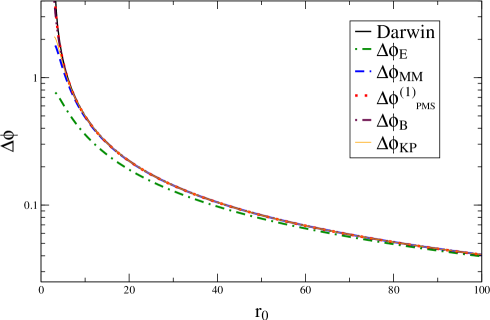
Figure 1: Deflection angle as a function of $r_{0}$ assuming $GM=1$. (color online)

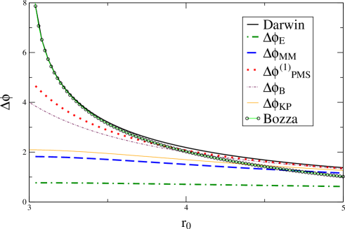
Figure 2: Deflection angle as a function of $r_{0}$ assuming $GM=1$ close to the photon sphere. (color online)

In Fig. 3 we also show the magnification (see Mutkaa )

$$\mu=\left|\left(1+\frac{a}{b}\Delta\phi\right)\left(1+a\frac{\partial r_{0}}{\partial b}\frac{\partial\Delta\phi}{\partial r_{0}}\right)\right|^{-1}\ ,$$ (35)

as a function of the impact parameter $b$. $a$ is the distance between the lens and the source. Once again our simple formula provides a very accurate approximation to the exact result over a wide range of values.

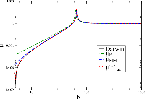
Figure 3: Magnification as a function of the impact parameter assuming $a=1000$ and $GM=1$. (color online)

Given the success of our approach to first order, a higher order calculation is not essential, although it is not technically difficult. For example, it is straightforward to obtain the second order formula

$$\Delta\phi_{PMS}^{(2)}=\frac{\pi\left(15\pi^{2}\left(\Lambda^{2}-1\right)^{2}-16\pi\left(\Lambda^{2}-1\right)^{2}-32\left(8\Lambda^{5}-5\Lambda^{4}-6\Lambda^{2}+3\right)\right)}{256\Lambda^{5}}$$ (36)

where

$$\Lambda \equiv \sqrt{\lambda_{PMS}^{(1)}}=\sqrt{1-\frac{8GM}{\pi r_{0}}}\ .$$ (37)

This formula approximates the deflection angle to a $1\%$ level up to $r_{0}\approx 3.5\ GM$, i.e. quite close to the singularity, compared to $r_{0}\approx 7.4\ GM$ of the first order result.

Using the results obtained in Section III we can also estimate the rate of convergence of our series. In this case the potential is

$$V(z)=z^{2}-\frac{2GM}{r_{0}}z^{3}\ ,$$ (38)

and

$$\Delta_{max}=\frac{GM/r_{0}}{2-5GM/r_{0}}\ .$$ (39)

It is interesting to notice that the condition of applicability of our series, $\lambda_{max}>\lambda_{C}$, can be fulfilled only for $r_{0}>3GM$, which is the exact location of the photon sphere for the Schwarzschild metric: in other words, our series can also describe strong gravitational lensing close to the photon sphere.

IV.2 Reissner-Nordström metric

The Reissner-Nordström (RN) metric describes a black hole with charge and corresponds to

$$B(r)=A^{-1}(r)=\left(1-\frac{2GM}{r}+\frac{Q^{2}}{r^{2}}\right)\ \ \ \ D(r)=1\ .$$ , (40)

As for the Schwarzschild metric the angle of deflection of a ray of light reaching a minimal distance $r_{0}$ from the black hole can be obtained from eq. (2). Eiroa, Romero and Torres Eir02 have been able to express the deflection angle in terms of elliptic integrals of the first kind (see eqn. (A3) of Eir02 ).

It is straightforward to use our general formula to obtain the transformed potential for the RN metric

$$\rho(1)=\frac{\pi}{2}-\frac{4GM}{r_{0}}+\frac{3\pi Q^{2}}{4r_{0}^{2}}$$ (41)

and thus the deflection angle

$$\Delta\phi_{PMS}^{(1)}=\pi\left[\frac{1}{\sqrt{1-\frac{8GM}{\pi r_{0}}+\frac{3Q^{2}}{2r_{0}^{2}}}}-1\right]\ .$$ (42)

We can compare our formula both with the exact analytical result of Eiroa et al. and with the expressions (47) and (53) of Keet05 , which provide a systematic expansion of the deflection angle in terms of $GM/b$. In Fig. 4 we have plotted the exact solution of Eir02 together with our first order formula and with the expression of Keeton and Petters, assuming $G=M=1$ and $Q=1/2$: the reader can appreciate that our simple formula is very accurate even in proximity of the photon sphere.

Notice that our expression reproduces well also the asymptotic behaviour of the deflection angle. In fact, eq. (19) of Bha03 provides the leading asymptotic behavior of $\Delta\phi$, valid for $r\rightarrow\infty$:

$$\Delta\phi \approx \frac{4GM}{r_{0}}+\frac{4G^{2}M^{2}}{r_{0}^{2}}\left(\frac{15\pi}{16}-1\right)-\frac{3\pi}{4}\frac{Q^{2}}{r_{0}^{2}}+O\left[\left(\frac{1}{r_{0}}\right)^{2}\right]$$ (43)

$$\approx \frac{4GM}{r_{0}}+7.78\ \frac{G^{2}M^{2}}{r_{0}^{2}}-2.36\ \frac{Q^{2}}{r_{0}^{2}}+O\left[\left(\frac{1}{r_{0}}\right)^{2}\right]\ .$$

which can be compared with the asymptotic behaviour of our formula

$$\Delta\phi_{PMS}^{(1)} \approx \frac{4GM}{r_{0}}+\frac{24G^{2}M^{2}}{\pi r_{0}^{2}}-\frac{3\pi}{4}\frac{Q^{2}}{r_{0}^{2}}+O\left[\left(\frac{1}{r_{0}}\right)^{2}\right]$$ (44)

$$\approx \frac{4GM}{r_{0}}+7.64\ \frac{G^{2}M^{2}}{r_{0}^{2}}-2.36\ \frac{Q^{2}}{r_{0}^{2}}+O\left[\left(\frac{1}{r_{0}}\right)^{2}\right]\ .$$

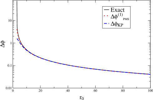
Figure 4: Deflection angle for the Reissner-Nordström metric as a function of $r_{0}$ assuming $GM=1$ and $Q=1/2$. (color online)

Once again we can refer to the results of Section III to estimate the rate of convergence of our series. In this case the potential is

$$V(z)=z^{2}-\frac{2GM}{r_{0}}z^{3}+\frac{Q^{2}}{r_{0}^{2}}z^{4}\ ,$$ (45)

and

$$\Delta_{max}=\frac{GM/r_{0}-Q^{2}/r_{0}^{2}}{2-5GM/r_{0}+3Q^{2}/r_{0}^{2}}\ .$$ (46)

In this case, the condition of applicability of our series, $\lambda_{max}>\lambda_{C}$, can be fulfilled only for $r_{0}>3GM/2\left(1+\sqrt{1-8/9(Q/GM)^{2}}\right)$, which is the exact location of the photon sphere for the Reissner-Nordström metric (see eq.(8) of Eir02 ).

IV.3 Janis-Newman-Winicour metric

We consider now the spherically symmetric metric solution to the Einstein massless scalar equations JNW68 :

$$A(r)=\left(1-b/r\right)^{-\nu}\ \ \ ,\ \ \ B(r)=\left(1-b/r\right)^{\nu}\ \ \ ,\ \ \ D(r)=\left(1-b/r\right)^{1-\nu}\ ,$$ (47)

which reduces to the Schwarzschid metric for $\nu=1$ and for $b=GM$. In this case we obtain the potential

$$V(z) = -\left(1-\frac{b}{r_{0}}\right)^{2\nu-1}\left(1-\frac{bz}{r_{0}}\right)^{2-2\nu}+z^{2}\left(1-\frac{bz}{r_{0}}\right)+\left(1-\frac{b}{r_{0}}\right)^{2\nu-1}$$ (48)

which can be expanded around $z=0$ to give

$$V(z) \approx -2(\nu-1)(1-\frac{b}{r_{0}})^{2\nu-1}\frac{b}{r_{0}}z+\left[1-(\nu-1)(2\nu-1)\left(1-\frac{b}{r_{0}}\right)^{2\nu-1}\left(\frac{b}{r_{0}}\right)^{2}\right]\ z^{2}$$ (49)

$$+ \left[-\frac{2}{3}(\nu-1)\nu(2\nu-1)\left(\frac{b}{r_{0}}\right)^{3}\left(1-\frac{b}{r_{0}}\right)^{2\nu-1}-\frac{b}{r_{0}}\right]\ z^{3}+O\left[z^{4}\right]\ .$$

Using this expansion inside our formula, eq. (17), we obtain the deflection angle

$$\Delta\phi_{PMS}^{(1)}=\pi\ \left[\frac{1}{\sqrt{1+\frac{(\nu-1)(1-\xi)^{2\nu}\xi((2\nu-1)\xi(8\nu\xi+3\pi\ )+12)-12(\xi-1)\xi}{3\pi(\xi-1)}}}1-\right]$$ (50)

where $\xi\equiv b/r_{0}$.

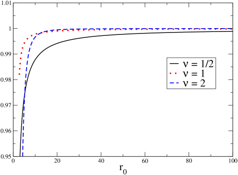
Figure 5: Ratio between the approximate first order formula and the exact (numerical) result in the JNW metric for different values of $\nu$ and assuming $b=1$. The potential is expanded to order $z^{3}$. (color online)

In fig. 5 we have plotted the ratio $\Delta\phi_{PMS}^{(1)}/\Delta\phi_{exact}$ for three values of $\nu$, up to small values of $r_{0}$. Notice that the exact result is calculated numerically and that the ratio is close to $1$ up to very small values of $r_{0}$.

The expansion of eq. (50) around $r_{0}$ reads

$$\Delta\phi_{PMS}^{(1)}\approx\frac{2b\nu}{r_{0}}+\frac{\left(2\left(6-4\pi+\pi^{2}\right)\nu^{2}-3(-4+\pi)\pi\nu+(-4+\pi)\pi\right)}{2\pi}\frac{b^{2}}{r_{0}^{2}}+O\left[1/r_{0}^{3}\right]\ ,$$ (51)

and provides a deviation from Einstein’s leading order term, $\Delta\phi\approx 2b/r_{0}$ for $\nu\neq 1$.

IV.4 Einstein-Born-Infeld black holes

As a final example of application of our method we consider the propagation of light in a charged black hole coupled to Born-Infeld electrodynamics. This problem has been recently considered by Eiroa in Eir06 and corresponds to the effective metric

$$A(r)=\frac{\sqrt{\omega(r)}}{\psi(r)}\ \ ,\ \ B(r)=\sqrt{\omega(r)}\psi(r)\ \ ,\ \ D(r)=\frac{1}{\sqrt{\omega(r)}}\ ,$$ (52)

where

$$\omega(r) = 1+\frac{Q^{2}b^{2}}{r^{4}}$$ (53)

$$\psi(r) = 1-2\frac{M}{r}+\frac{2}{3b^{2}}\ \left\{r^{2}-\sqrt{r^{4}+b^{2}Q^{2}}+\frac{\sqrt{|bQ|^{3}}}{r}\ F\left[\arccos\left(\frac{r^{2}-|bQ|}{r^{2}+|bQ|}\right),\frac{1}{\sqrt{2}}\right]\right\}\ .$$ (54)

$F(a,b)$ is the incomplete elliptic integral of first kind. We follow the convention of Eir06 and set $G=1$.

In this case one obtains the potential

$$V(z) \equiv z^{2}\frac{\psi(r_{0}/z)}{\omega(r_{0}/z)}-\frac{\psi(r_{0})\omega(r_{0})}{\omega^{2}(r_{0}/z)}+\psi(r_{0})\omega(r_{0})$$ (55)

which can be expanded around $z=0$ as

$$V(z)=\sum_{n=2}^{\infty}v_{n}z^{n}\ .$$ (56)

Unlike in the previous two cases $V(z)$ is not polynomial in $z$ and the deflection angle reads

$$\Delta\phi_{PMS}^{(1)} = \pi\ \left[\frac{1}{\sqrt{1-\frac{8M}{\pi r_{0}}+\frac{3}{2}v_{4}+\frac{16}{3\pi}v_{5}+\frac{15}{8}v_{6}+\dots}}-1\right]$$ (57)

Clearly one has to keep in mind that the truncation of the series (56) to a finite order is an additional source of error in our calculation: in practice, however, it is straightforward to include further terms of the expansion.

In Fig. 6 we have compared the exact result obtained numerically integrating the integral in $\Delta\phi$ with the result obtained with our first order formula using the expansion $V(z)$ to order $z^{4}$:

$$V(z)\approx z^{2}-\frac{2M}{r_{0}}z^{3}+v_{4}z^{4}+O[z^{5}]$$ (58)

where

$$v_{4} = \frac{7Q^{2}}{3r_{0}^{2}}+\frac{2}{3}\left(3b^{2}-2\beta\right)\frac{Q^{2}}{r_{0}^{4}}+\frac{4}{3}\frac{bQ^{2}}{r_{0}^{5}}\left(\gamma Q\sqrt{bQ}-3bM\right)+\frac{4b^{2}Q^{4}}{3r_{0}^{6}}$$ (59)

$$+ \frac{2}{3}b^{2}\left(3b^{2}-2\beta\right)\frac{Q^{4}}{r_{0}^{8}}+\frac{4Mb^{4}Q^{4}}{r_{0}^{9}}\ \left(\frac{\gamma Q^{3/2}}{3\sqrt{b}M}-1\right)$$

and

$$\beta^{2} \equiv b^{2}Q^{2}+r_{0}^{4}$$ (60)

$$\gamma \equiv F\left(\arccos\left(1-\frac{2bQ}{r_{0}^{2}+bQ}\right),\frac{1}{\sqrt{2}}\right)\ .$$ (61)

Our analytical formula reproduces with high accuracy the numerical result obtained assuming $b=M=1$ and $Q=1/2$.

It is also easy to obtain the asymptotic behavior of $\Delta\phi$ from our expression

$$\Delta\phi\approx\frac{4M}{r_{0}}+\left(\frac{24}{\pi}\frac{M^{2}}{r_{0}^{2}}-\frac{3\pi}{4}\frac{Q^{2}}{r_{0}^{2}}\right)+\left(\frac{160}{\pi^{2}}\frac{M^{3}}{r_{0}^{3}}-9\frac{MQ^{2}}{r_{0}^{3}}\right)+O\left[\frac{1}{r_{0}^{4}}\right]\ .$$ (62)

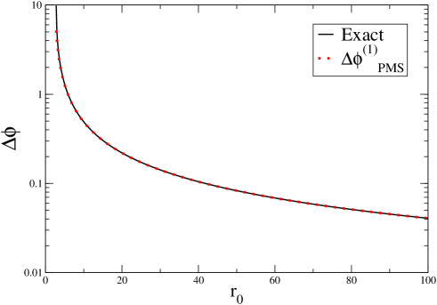
Figure 6: Deflection angle for the Einstein-Born-Infeld problem as a function of $r_{0}$ assuming $b=M=1$ and $Q=1/2$. The potential in our formula is expanded to order $z^{4}$. (color online)

V Conclusions

In this paper we have presented a new method to obtain analytical expressions for the deflection angle of a ray of light propagating in a spherically symmetric static metric. We have been able to prove the convergence of our approach and to estimate the rate of convergence of the series obtained applying our method: the series converges exponentially and can be applied over all the physical region, as explictly seen in the case of the Schwarzschild and Reissner-Nordström metrics, where the correct location of the photon sphere is recovered.

This method has been used to derive a first order formula, which is valid for general spherically symmetric static metric tensor: we have tested this formula in four different cases, observing that it is quite accurate even in proximity of the photon sphere. Clearly, higher order corrections to the first order formula of this paper will further improve the quality approximation, given the convergent nature of our expansion: we plan to study higher order corrections to our formula in a forthcoming paper.

We also stress that the series obtained with our method are nonperturbative, because they do not correspond to an expansion in a small parameter and therefore they are capable of providing small errors even when the parameters in the model are not small (a typical perturbative parameter would be $GM/r_{0}$).

- (1) S. Frittelli, T.P. Kling and T.Newman, Phys.Rev.D 61, 064021 (2000)
- (2) K.S.Virbhadra and G.F.R.Ellis,Phys. Rev. D 62, 084003 (2000)
- (3) K.S.Virbhadra and G.F.R.Ellis,Phys. Rev. D 65, 103004 (2002)
- (4) E.F.Eiroa,G.E.Romero and D.F.Torres, Phys. Rev. D 66, 024010 (2002)
- (5) A. Bhadra, Phys. Rev. D 67, 103009 (2003)
- (6) V. Bozza, Phys. Rev. D 67, 103006 (2003); V. Bozza, F. De Luca, G. Scarpetta, M. Sereno, Phys.Rev. D72, 08300 (2005)
- (7) R. Whisker, Phys. Rev. D 71, 064004 (2005)
- (8) E.F. Eiroa, Phys. Rev. D 71, 083010 (2005)
- (9) E.F.Eiroa, Phys. Rev. D 72, 043002 (2006)
- (10) K. Sarkar and A. Bhadra, ArXiv:[gr-qc/0602087] (2006)
- (11) V. Perlick, Phys.Rev. D 69, 064017 (2004)
- (12) V.Bozza, Phys. Rev. D 66, 103001 (2002)
- (13) P.T. Mutka and P. Mähönen, The Astrophysical Journal 581: 1328-1336 (2002)
- (14) P.T. Mutka and P. Mähönen, The Astrophysical Journal 576: 107-112 (2002)
- (15) A.M. Beloborodov, The Astrophysical Journal 566: L85-L88 (2002)
- (16) C.R. Keeton and A.O. Petters, Phys. Rev. D 72, 104006 (2005)
- (17) P.Amore and R.A.Saénz, Europhysics letters 70 425-431 (2005)
- (18) P.Amore, A.Aranda, F.Fernandez and R.A.Saénz, Phys. Rev.E 71 (2005)
- (19) A. Okopińska, Phys. Rev. D 35, 1835 (1987); A. Duncan and M. Moshe, Phys. Lett. B 215, 352 (1988); H.F.Jones and M. Moshe, Phys. Lett. B 234, 492 (1990)
- (20) H. Kleinert, Path Integrals in Quantum Mechanics, Statistics and Polymer Physics, 3rd edition (World Scientific Publishing, 2004)
- (21) P.M. Stevenson, Phys. Rev. D 23, 2916 (1981)
- (22) S. Weinberg, Gravitation and cosmology, J.Wiley and Sons, 1972
- (23) C. Darwin, Proc.R. Soc. London A 249, 180 (1959); C. Darwin, Proc.R. Soc. London A 263, 39 (1961);
- (24) P. Amore, A. De Pace and J. Lopez, submitted to Jour. of Phys. G: ArXiv:[hep-ph/0602114] (2006)
- (25) P. Amore, accepted on the Journal of Mathematical analysis and applications, ArXiv:[math-ph/0408036], (2006)
- (26) P. Amore, J. of Phys. A 38, 6463-6472 (2005)
- (27) A.I.Janis, E.T.Newman and J.Winicour, Phys.Rev.Lett. 20, 878 (1968)