A multi-block infrastructure for three-dimensional time-dependent numerical relativity

Abstract

We describe a generic infrastructure for time evolution simulations in numerical relativity using multiple grid patches. After a motivation of this approach, we discuss the relative advantages of global and patch-local tensor bases. We describe both our multi-patch infrastructure and our time evolution scheme, and comment on adaptive time integrators and parallelisation. We also describe various patch system topologies that provide spherical outer and/or multiple inner boundaries.

We employ penalty inter-patch boundary conditions, and we demonstrate the stability and accuracy of our three-dimensional implementation. We solve both a scalar wave equation on a stationary rotating black hole background and the full Einstein equations. For the scalar wave equation, we compare the effects of global and patch-local tensor bases, different finite differencing operators, and the effect of artificial dissipation onto stability and accuracy. We show that multi-patch systems can directly compete with the so-called fixed mesh refinement approach; however, one can also combine both. For the Einstein equations, we show that using multiple grid patches with penalty boundary conditions leads to a robustly stable system. We also show long-term stable and accurate evolutions of a one-dimensional non-linear gauge wave. Finally, we evolve weak gravitational waves in three dimensions and extract accurate waveforms, taking advantage of the spherical shape of our grid lines.

I Introduction

Many of the spacetimes considered in numerical relativity are asymptotically flat. An ideal kind of domain for these has its boundaries at infinity, and at the same time has to handle singularities which exist or develop within the domain. In a realistic setup, the outer boundary is either placed at infinity, which is topologically a sphere, or one introduces an artificial outer boundary at some large distance from the origin. In both cases, a sphere is a natural shape for the boundary.

There are several possible ways to deal with singularities. One of the most promising is excision, which was first used by J. Thornburg Thornburg (1987), where he acknowledges W. G. Unruh for the idea. Excision means introducing a inner boundary, so that the singularity is not in the computational domain any more. If done properly, all characteristic modes on this inner boundary are leaving the domain, so that no physical boundary condition is required. Seidel and Suen Seidel and Suen (1992) applied this idea for the first time in a spherically symmetric time evolution.

A well posed initial boundary value problem requires in general smooth boundaries Secchi (1996). Using spherical boundaries satisfies all conditions above. Spherical boundaries have not yet been successfully implemented in numerical relativity with Cartesian grids. However, there were many attempts to approximate spherical boundaries. For example, the Binary Black Hole Grand Challenge Alliance used blending outer boundary conditions Rezzolla et al. (1999); Brandt et al. (2000), where the blending zone was approximately a spherical shell on a Cartesian grid. Excision boundaries often approximate a sphere by having a Lego (or staircase) shape Brandt et al. (2000); Shoemaker et al. (2003); Alcubierre et al. (2004a); Sperhake et al. (2005). Some of the problems encountered with excision are attributed to this staircase shape. A spherical boundary would be smooth in spherical coordinates, but these are undesirable because they have a coordinate singularity on the $z$ axis. A multi-block scheme allows smooth spherical boundaries without introducing coordinate singularities.

Using multiple grid patches is a very natural thing to do in general relativity. When one starts out with a manifold and wants to introduce a coordinate system, then it is a priori not clear whether a single coordinate system can cover all the interesting parts of the manifold. One usually introduces a set of overlapping maps, each covering a part of the manifold. After discretising the manifold, one arrives naturally at multiple grid patches.

Methods using multiple grid patches in numerical relativity were pioneered in 1987 by J. Thornburg Thornburg (1987, 1993), where he also introduced excision as inner boundary condition for black holes. Gómez et al. Gómez et al. (1997) use two overlapping stereographic patches to discretise the angular direction using the eth formalism. This was later used by Gómez et al. Gómez et al. (1998) to evolve a single, non-stationary black hole in a stable manner in three dimensions with a characteristic formulation. Thornburg Thornburg (2004) evolves a stationary Kerr black hole in three dimensions using multiple grid patches using a Cauchy formulation. Kidder, Pfeiffer, and Scheel Kidder et al. (2005a) have developed a multi-patch pseudospectral code to evolve first-order hyperbolic systems on conforming (neighboring patches share grid points), touching, and overlapping patches. Scheel et al. Scheel et al. (2004) used this method with multiple radial grid patches to evolve a scalar field on a Kerr background. Kidder et al. Kidder et al. (2005b) used this method with multiple radial grid patches to evolve a distorted Schwarzschild black hole.

In this paper, we describe a generic infrastructure for time evolution simulations in numerical relativity using multiple grid patches, and we show example applications of this infrastructure. We begin by defining our notation and terminology in section II, where we also discuss various choices that one has to make when using multi-patch systems. We describe our infrastructure in section III and the patch systems we use in section IV. We test our methods with a scalar wave equation on flat and curved backgrounds and with the full vacuum Einstein equations in sections V and VI. We close with some remarks on future work in section VII.

II Multi-patch systems

Our main motivation for multi-patch systems is that they provide smooth boundaries without introducing coordinate singularities. This allows us to implement symmetric hyperbolic systems of equations for well posed initial boundary value problems. However, multi-patch systems have three other large advantages when compared to using a uniform Cartesian grid.

No unnecessary resolution. In multi-patch systems the angular resolution does not necessarily increase with radius. An increasing angular resolution is usually not required, and multi-patch systems are therefore more efficient by a factor $O(n^{2})$ when there are $O(n^{3})$ grid points.

No CFL deterioration for co-rotating coordinates. When a co-rotating coordinate system is used, the increasing angular resolution in Cartesian grids forces a reduction of the time step size. Near the outer boundary, the co-rotation speed can even be superluminal. This does not introduce any fundamental problems, except that the time step size has to be reduced to meet the CFL criterion. This makes Cartesian grids less efficient by a factor of $O(n)$ for co-rotating coordinate systems when there are $O(n^{3})$ grid points.

Convenient radially adaptive resolution. In multi-patch systems, it is possible to vary the radial resolution without introducing coordinate distortions Thornburg (2004). This is not possible with Cartesian coordinates. Fish-eye coordinate transformations Baker et al. (2002) lead to distorted coordinate systems. In practise, there is a limit to how large a fish-eye transformation can be, while there is no such limit for a radial rescaling in multi-patch systems.

These advantages are so large that we think that fixed mesh refinement methods may even be superfluous for many applications in numerical relativity. Mesh refinement can be used adaptively, e.g. to resolve shock waves in a star. It would be difficult to handle this with adaptive patch systems. However, mesh refinement is also used statically to have higher resolution in the centre and lower resolution near the outer boundary. This case is very elegantly handled by multi-patch systems. Multi-patch systems could also be used to track moving features, such as orbiting black holes.

II.1 Terminology

Methods using multiple grid patches are not yet widely used in numerical relativity, and this leads to some confusion in terminology.

The notions of multiple patches, multiple blocks, or multiple maps are all virtually the same. In differential geometry, one speaks of maps covering a manifold. In computational physics, one often speaks of multi-patch systems when the patches overlap, and of multi-block systems if they only touch, i.e., if the blocks only have their boundaries in common. However, when discretised, there is an ambiguity as to what part of the domain is covered by a grid with a certain resolution. See figure 1 for an illustration.

In the following, we say that a grid extends from its first to its last grid point. This is different from Thornburg’s notation Thornburg (2004): He divides the grid into interior and ghost points. The interior points are evolved in time, and a small number of ghost points are defined through an inter-patch boundary condition, which is interpolation in his case. He defines the grid extent as ranging from the first to the last interior point, ignoring the ghost points for that definition. Thus, when there are $n$ ghost points, he calls “touching” what we would call an “overlap of $2n$ points”. When he speaks of overlapping grids according to his definition, then there are parts of the domain covered multiple times, and these overlap regions do not vanish in the continuum limit.

(a) Touching patches, also known as blocks.

(b) Touching patches with additional boundary points.

(c) Overlapping patches with boundary points.

Figure 1: Schematics of the difference between touching and overlapping grids for different inter-grid relations. The black grid points are evolved in time, the hollow grid points are determined via a boundary condition.

II.2 Coordinates and tensor bases

Although not strictly necessary, it is nevertheless very convenient to have one global coordinate system covering the whole domain. This makes it very easy to set up initial conditions from known analytic solutions, and it also makes it possible to visualise the result of a simulation. While a true physics-based visualisation would not rely on coordinates, currently used methods always display fields with respect to a coordinate system.

Since our calculations concern quantities that are not all scalars, we have to make a choice as to how to represent these. One elegant solution is to use a tetrad (or triad) formalism, where one represents vectorial and tensorial quantities by their projections onto the tetrad elements. However, this still leaves open the choice of tetrad elements.

In a multi-patch environment there are two natural choices for a coordinate basis. One can either use the global or the patch-local coordinate system. Both have advantages and disadvantages.

In a way, using a patch-local coordinate basis is the more natural choice. Given that one presumably knows how to evolve a system on a single patch, it is natural to view a multi-patch system just as a fancy outer boundary condition for each patch. In this way, one would continue to use patch-local coordinates everywhere, while the inter-patch boundary conditions involve the necessary coordinate transformations. It should be noted that these coordinate transformations mix the evolved variables, because (e.g. for a vector $v_{i}$) what is $v_{1}$ on one patch is generally a linear combination of all $v_{i}$ in the other patches’ coordinate system.

Using a global coordinate basis corresponds to defining a global triad that is smooth over the entire domain. This simplifies the inter-patch boundary conditions significantly, since there is no coordinate transformation necessary. Instead, one then has to modify the time evolution mechanism on the individual patches:

Let the letters $a,b,c\ldots$ denote abstract indices for quantities in the patch-local tensor basis, and letters $i,j,k\ldots$ abstract indices in the global tensor basis. The triad that defines the global tensor basis is given by $e_{a}^{i}$, which is a set of one-forms $e_{a}$ labelled by a global index $i$. A vector field $\mathbf{v}$ is denoted $v^{a}$ in the patch-local tensor basis and $v^{i}:=e_{a}^{i}v^{a}$ in the global tensor basis. Note that $v^{i}$ transforms as a scalar with respect to the patch-local tensor basis, as a change in the patch-local tensor basis does not change $v^{i}$.

When one calculates partial derivatives, e.g. through finite differences, one obtains these always in the patch-local coordinate basis. It is then necessary to transform these to the global coordinate basis. Since the evolved variables are scalars with respect to the patch-local coordinate basis, their first derivatives are co-vectors, and their transformation behaviour is straightforward:

$$\partial_{i} = \frac{\partial x^{a}}{\partial x^{i}}\,\partial_{a}$$ (1)

where $\partial x^{a}/\partial x^{i}=(\partial x^{i}/\partial x^{a})^{-1}=(e_{a}^{i})^{-1}$ is the (inverse) Jacobian of the coordinate transformation. This means that using a global tensor basis effectively changes the system of evolution equations.

Using a global coordinate basis also has advantages in visualisation. Visualisation tools generally expect non-scalar quantities to be given in a global coordinate basis. Often, one also wants to examine certain components of non-scalar quantities, such as e.g. the radial component of the shift vector. When the shift vector is given in different coordinate bases on each patch, then the visualisation tool has to perform a non-trivial calculation.

It should be noted that there are many quantities which have a non-tensorial character, such as e.g. the quantities $d_{kij}$ of the formulation introduced in Sarbach and Tiglio (2002) which we use below; $d_{kij}$ are partial derivatives of the three-metric. The quantities $\phi$ and $\tilde{\Gamma}^{i}$ of the BSSN formalism Alcubierre et al. (2000) have an even more complex transformation behaviour. $\phi=\ln\sqrt[12]{\det(\gamma_{ij})}$ is the logarithm of a scalar density, and $\tilde{\Gamma}^{i}=\tilde{\gamma}^{jk}\tilde{\Gamma}^{i}_{jk}$ is a partial derivative of a tensor density.

It is also necessary to define the set of characteristic variables at an inter-patch boundary in an invariant manner. One convenient way to do so is again to refer to a global coordinate basis. That is, one transforms the elements of the state vector to the global coordinate basis, and can then define the characteristic variables in a unique way.

Last but not least, there is one more compelling argument for using a global coordinate basis to represent the state vector. Since one, presumably, already knows how to evolve the system within a single patch, it may be unwise to place all the new complications that a multi-patch system brings into the inter-patch boundary condition. By changing the evolved system to use a global coordinate basis, one simplifies the inter-patch boundaries significantly, and furthermore one can implement and test both steps separately.

III Infrastructure

We base our code on the Cactus framework Goodale et al. (2003); cac (a) using the Carpet infrastructure Schnetter et al. (2004); car . Cactus is a framework for scientific computing. As a framework, the core (“flesh”) of Cactus itself contains no code that does anything towards solving a physics problem; it contains only code to manage modules (“thorns”) and let them interact. Cactus comes with a set of core thorns for basic tasks in scientific computing, including time integrators and a parallel driver for uniform grids. (A driver is responsible for memory allocation and load distribution on parallel machines.)

By replacing and adding thorns, we have extended Cactus’ capabilities for multi-patch simulations. The mesh refinement driver Carpet can now provide storage, inter-processor communication, and I/O for multi-patch systems as well, and the multi-patch and mesh refinement infrastructures can be used at the same time. The definitions of the patch systems (see below) and the particular inter-patch boundary conditions are handled by additional thorns.

III.1 Infrastructure description

A computation that involves multiple patches requires implementing several distinct features. We decided to split this functionality across multiple modules, where each module is implemented as a Cactus thorn. These are

Driver (D):

The driver is responsible for memory allocation and load distribution, for inter-processor communication, and for I/O. It also contains the basic time stepping mechanism, ensuring that the application e.g. updates the state vector on each patch in turn.

Multi-patch system (MP):

The patch system selects how many patches there are and how they are connected, i.e., which face is connected to what face of which other patch, and whether there is a rotation or reflection necessary to make the faces match. The patch system also knows where the patches are located in the global coordinate space, so that it can map between patch-local and global coordinates.

Penalty boundaries (P):

This thorn applies a penalty boundary condition to the right hand side (RHS) of the state vector of one face of one patch. We have described the details in Diener et al. (2005). It calls other routines to convert the state vector and its RHS on the patch and on its neighbour to and from their characteristic variables; it is thus independent of the particular evolution system.

Finite differences (FD):

As a helper module, we implemented routines to calculate high order finite differences on the patches Diener et al. (2005). These operators use one-sided differencing near the patch boundaries.

Additionally, we make use of the following features that Cactus provides:

Time integrator (TI):

The time integrator calls user-provided routines that evaluate the RHS of the state vector, advances the state vector in time, and calls boundary condition routines.

Boundary conditions (BC):

The boundary condition infrastructure keeps track of what boundary conditions should be applied to what faces and to what variables. It distinguishes between inter-processor boundaries (which are synchronised by the driver), physical boundary conditions (where the user applies a condition of his/her choice), and symmetry boundary conditions (which are determined through a symmetry of the computational domain, e.g. a reflection symmetry about the equatorial plane). We have extended the notion of symmetry boundaries to also include inter-patch boundaries, which are in our case handled by the penalty method.

Together, this allows multi-patch systems to be evolved in Cactus within the existing infrastructure. Existing codes, which presumably only calculate the right hand side (RHS) and apply boundary conditions, can make use of this infrastructure after minimal changes, and after e.g. adding routines to convert the state vector from and to the characteristic modes. Existing codes which are not properly modular will need to be restructured before they can make use of this multi-patch infrastructure.

We use the penalty method to enforce the inter-patch boundary conditions. The penalty method for finite differences is described in Carpenter et al. (1994, 1999); Nordström and Carpenter (2001), and we describe our approach and notation in Diener et al. (2005).

In order to treat systems containing second (or higher) temporal derivatives with our current infrastructure, one needs to rewrite them to a form where only contain only first temporal derivatives by introducing auxiliary variables. This is always possible. Strongly or symmetric hyperbolic systems containing second (or higher) spatial derivatives Kreiss and Ortiz (2002); Sarbach et al. (2002); Nagy et al. (2004); Beyer and Sarbach (2004); Gundlach and Martin-Garcia (2005); Babiuc et al. (2006) could in principle also be handled without reducing them to first order. The definition of the characteristic modes has then to be adapted to such a formulation, and may then contain derivatives of the evolved variables.

This multi-patch approach is not limited in any way to finite differencing discretisations. It would equally be possible to use e.g. spectral methods to discretise the individual patches (as was done in Scheel et al. (2004).) It may even make sense to use structured finite element or finite volume discretisations on the individual patches, using a multi-patch system to describe the overall topology.

III.2 Initial condition, boundary conditions, and time evolution

We now describe how the initial conditions are set up and how the state vector is evolved in time. This explains in some more detail how the different modules interact, and what parts of the system have to be provided by a user of this multi-patch infrastructure. Each step is marked in parentheses (e.g. “(MP)”) with the module that performs that step.

Setting up the initial conditions proceeds as follows:

1. Initialise the patch system. (MP) The patch system is selected, and the location and orientation of the patches is determined depending on run-time parameters. If desired, the patch system specification is read from a file (see below).

2. Set up the global coordinates. (MP) For all grid points on all patches, the global coordinates are calculated. At this time we also calculate and store the Jacobian of the coordinate transformation between the global and the patch-local coordinate systems. If necessary, we also calculate derivatives of the Jacobian. Derivatives may be required to transform non-tensorial quantities when a patch-local tensor basis is used. The Jacobian can be calculated either analytically (if the coordinate transformation is known analytically) or numerically via finite differences.

3. Initialise the three-metric. (User code) Even when the evolved system does not contain the Einstein equations, we decided to use a three-metric. This is a convenient way to describe the coordinate system, which —even if the spacetime is flat— is non-trivial in distorted coordinates. For example, polar-spherical coordinates can be expressed using the three-metric $\gamma_{ij}=\mathrm{diag}\left(1,r^{2},r^{2}\sin^{2}\theta\right)$, and doing so automatically takes care of all geometry terms.

   This step is performed by the user code, and it is not necessary to use an explicit three-metric in order to use this infrastructure. At this time, we initialise the metric at the grid point locations, specifying its Cartesian components in the global tensor basis.

4. Initialise the state vector. (User code) Here we initialise the state vector of the evolution system, also again specifying its Cartesian components in the global tensor basis. When evolving Einstein’s equations, this step and the previous are combined.

5. Convert to local tensor basis (if applicable) (User code) It is the choice of the user code whether the state vector should be evolved in the global or in the patch-local tensor bases. We have discussed the advantages of either approach above. If the evolution is to be performed in patch-local coordinates, then we transform the three-metric and the state vector at this time. Note that this transformation does not require interpolation, since we evaluated the initial condition already on the grid points of the individual patches.

At this stage, all necessary variables have been set up, and the state vector is in the correct tensor basis.

The time evolution steps occur in the following hierarchical manner:

1. Loop over time steps. (D) The driver performs time steps until a termination criterion is met. At each time step, the time integrator is called.

   1. Loop over substeps. (TI) We use explicit time integrators, which evaluate the RHS multiple times and calculate from these the updated state vector.

      1. Evaluate RHS. (User code) The RHS of the state vector is calculated, using e.g. the finite differencing thorn.

      2. Apply boundary conditions to RHS. (BC) We decided to apply boundary conditions not to the state vector, but instead to its RHS. This is necessary for penalty boundaries, but is a valid choice for all other boundaries as well. In our simulations, we do not apply boundary conditions to the state vector itself, although this would be possible. Both the inter-patch and the outer boundary conditions are applied via the multi-patch infrastructure in a way we explain below.

      3. Update state vector. (TI) Calculate the next —or the final— approximation of the state vector for this time step.

      4. Apply boundary conditions to the state vector. (User code) In our case, nothing happens here, since we apply the boundary conditions to the RHS of the state vector instead.

   2. Analyse simulation state. (D) The driver calls various analysis routines, which e.g. evaluate the constraints, or calculate the total energy of the system, or output quantities to files.

The multi-patch thorn knows which faces of which patches are inter-patch boundaries and which are outer boundaries. Inter-processor boundaries are handled by the driver and need not be considered here. Symmetry boundary conditions (such as e.g. a reflection symmetry) are currently not implemented explicitly, but they can be trivially simulated by connecting a patch face to itself. This applies the symmetry boundary via penalties, which is numerically stable, but differs on the level of the discretisation error from an explicitly symmetry condition.

The boundary conditions are applied in the following way:

1. Loop over all faces of all patches. (MP) Traverse all faces, determining whether this face is connected to another patch or not. Apply the boundary condition for this face, which is in our case always a penalty condition.

   1. Apply a penalty to the RHS. (P) Apply a penalty term to the RHS of all state vector elements. This requires calculating the characteristic variables at the patch faces.

      1. Determine characteristic variables. (User code) Calculate the characteristic variables from the state vector on the patch to which the penalty should be applied. If applying an inter-patch boundary condition, calculate the characteristic variables from the other patches’ state vector as well. If this is an outer boundary, then specify characteristic boundary data.

      2. Apply penalty. (P) Apply the penalty correction to the characteristic variables.

      3. Convert back from characteristic variables. (User code) Convert the characteristic variables back to the RHS of the state vector.

The edges and corners of the patches require some care. In our scheme, the edges and corners of the patches have their inter-patch condition applied multiple times, once for each adjoining patch. In the case of penalty boundary conditions, the edge and corner grid points are penalized multiple times, and these penalties are added up. This happens for each patch which shares the corresponding grid points. We have described this in more detail in Diener et al. (2005).

For nonlinear equations, there is an ambiguity in the definitions of the characteristic variables and characteristic speeds on the inter-patch boundaries. Since we use the penalty method, the state vector may be different at the boundary points on both sides of the interface. When the metric is evolved in time, then it is part of the state vector, and it may be discontinuous across the interface. The definition of the characteristics depends on the state vector in the nonlinear case. It can thus happen that the characteristic speeds are all positive when calculated at the boundary point on one side of the interface, and all negative when calculated on the other side of the interface. One has to pay attention to apply the penalty terms in a consistent manner even if this is the case. In our scheme (as described above), we always calculate the characteristic information using the state vector on that side of the interface to which the penalty terms are applied. This scheme does not prefer either side of the interface, but it is not fully consistent for nonlinear equations.

Instead of using penalty terms to apply boundary conditions, one could also apply boundary conditions in other ways, e.g. through interpolation from other patches, or by specifying Dirichlet or von Neumann conditions. Our infrastructure is ready to do so, but we have not performed a systematic study of the relative advantages of e.g. penalty terms vs. interpolation.

III.3 Time integration

It is common in numerical relativity to use explicit time integration methods. These limit the time step size to a certain multiple of the smallest grid spacing in the simulation domain. In non-uniform coordinate systems, one has to determine the smallest grid spacing explicitly, since it is the proper distance between neighbouring grid points that matters, not the grid spacing in the patch-local coordinate systems, and the proper distance can vary widely across a patch. If the three-metric, lapse, or shift are time-dependent, then the proper distances between the grid points also vary with time.

Furthermore, the maximum ratio between the allowed time step size and the grid spacing depends not only on the system of evolution equations; it depends also on the spatial discretisation operators that are used, on the amount of artificial dissipation, and on the strength of the penalty terms. While all this can in principle be calculated a priori, it is time consuming to do so.

Instead, we often use adaptive time stepping, for example using the adaptive step size control of the Numerical Recipes (Press et al., 1986, chapter 16.2). One can specify a time integration accuracy that is much higher than the spatial accuracy, and thus obtain the convergence order according to the spatial discretisation. In practise, one would rather specify a time integration accuracy that is comparable to the spatial accuracy. Adaptive time stepping would also have the above advantages when used on a single Cartesian grid.

We would like to remark on a certain peculiarity of adaptive time stepping. With a fixed time step size, instabilities manifest themselves often in such a way that certain quantities grow without bound in a finite amount of simulation time. Numerically, one notices that these quantities become infinity or nan (not a number) at some point when IEEE semantics Goldberg (1991) are used for floating point operations. With an adaptive step size, this often does not happen. Instead, the step size shrinks to smaller and smaller values, until either the step size is zero up to floating point round-off error, or the time integrator artificially enforces a certain, very small minimum step size. In both cases, computing time is used without making any progress. This case needs to be monitored and detected.

III.4 Parallelisation

Our current implementation parallelises a domain by splitting and distributing each patch separately onto all available processors. This is not optimal, and it would be more efficient to split patches only if there are more processors than patches, or if the patches have very different sizes. This is a planned future optimisation.

We have performed a scaling test on multiple processors. We solve a simple test problem on a patch system with multiple patches and measure the time it takes to take 100 time steps. As we increase the number of processors, we also increase the number of grid points, so that the load per processors remains approximately constant. This is realistic, because one chooses the number of processors that one uses for a job typically depending on the problem size. Figure 2 shows the results of the scaling tests for two such problem sizes. We find that our implementation scales well up to at least 128 processors, and would probably continue to scale to larger numbers. See cac (b) for a comparison of other benchmarks using Cactus and Carpet.

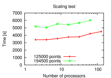
Figure 2: Wall clock time vs. numbers of processors for $100$ time steps of a test problem. We keep the load of each processor approximately constant at $125000$ and $194500$ grid points, respectively. Our implementation scales up to at least 128 processors.

It would also be possible to distribute the domain onto the available processors by giving (at least) one domain to each processor. This would mean that one splits domains when one adds more processors, introducing additional inter-patch boundary conditions. Penalty inter-patch boundary conditions are potentially more efficient than using ghost zones, since they require an overlap of only one single grid point. An $n$th order accurate finite differencing scheme, on the other hand, requires in general an overlap of $2n$ grid points. Penalty boundary conditions thus require less communication between the patches. A disadvantage of this scheme is that the exact result of a calculation then depends on the number of processors. Of course, these differences are only of the order of the discretisation error.

Such differences are commonly accepted when e.g. elliptic equations are solved. Many efficient algorithms for solving elliptic equations apply a domain decomposition, assigning one domain to each processor, and using different methods for solving within a domain and for coupling the individual domains. The discretisation error in the solution depends on the number of domains. For hyperbolic equations that are solved with explicit time integrators, it is often customary to not have such differences. On one hand, this may not be necessary to achieve an efficient implementation, and on the other hand, it simplifies verifying the correctness of a parallel implementation if the result is independent of the number of processors. However, there are no fundamental problems in allowing different discretisation errors when solved on different numbers of processors, especially if this may lead to a more efficient implementation.

IV Patch systems

We have implemented a variety of patch systems, both for testing and for standard application domains. It is also possible to read patch systems from file.

Simple testing patch systems are important not only while developing the infrastructure itself, but also while developing applications later on. Since the application has to provide certain building blocks, such as e.g. routines that convert to and from the characteristic representation, it is very convenient to test these in simple situations. Many patches have distorted local coordinate systems, and it is therefore also convenient to have patches with simple (one-dimensional) coordinate distortions. This can be used to test the tensor basis transformations — keeping in mind that some variables will not be tensorial, but will rather be tensor densities, or partial derivatives of tensors, with correspondingly more involved transformation behaviours.

We have currently two types of realistic patch systems implemented:

Six patches:

This system consists of six patches that cover a spherical shell, i.e., a region with $r_{\text{min}}\leq r\leq r_{\text{max}}$. We use the same patch-local coordinates as in Lehner et al. (2005) and Diener et al. (2005). This system is useful if the origin is not part of the domain, e.g. for a single black hole. See figure 3 for an illustration.

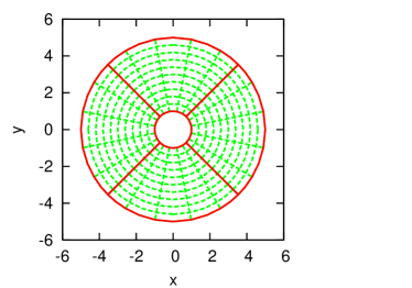
Figure 3: A cut in the equatorial plane of six patches, in which four patches are visible. The outer and inner domain boundaries are spheres. There is one radial coordinate spanning $r=\text{const}$ surfaces, and two angular coordinates perpendicular to that. The radial coordinate is smooth across patch boundaries.

Seven patches:

This system consists of one cubic patch that covers the region near the origin, and six additional patches that cover the exterior of the cube until a certain radius $r_{\text{max}}$. We use the same patch-local coordinates as in Diener et al. (2005), which are derived from the six-patch coordinates above. This system is useful if the origin should be part of the domain, e.g. for a single neutron star. See figure 4 for an illustration.

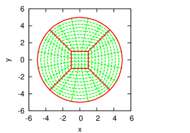
Figure 4: A cut in the equatorial plane of seven patches, in which five patches are visible. The outer boundary is a sphere, the inner patch is a cube. There is again one radial coordinate, but it does not span $r=\text{const}$ surfaces and it is not smooth across patch boundaries except at the outer boundary. The two angular coordinates are the same as in the six-patch system.

In addition to these two types, we have variations thereof, e.g. a system consisting of only one of the six patches assuming a sixfold reflection symmetry. We have individual patch types as generic building blocks, and we can glue them together to form arbitrary patch systems.

After seeking input from the computational fluid dynamics community, where multi-block systems are commonly used to obtain body-fitted coordinate systems, we decided that setting up patch systems by hand is too tedious, and that commercial tools should be used for that instead. We therefore implemented a patch system reader that understands the GridPro gri data format. This is a straightforward ASCII based format which is specified in the GridPro documentation, and support for other data formats could easily be implemented as well.

Using GridPro, we could easily import patch systems with two holes and 27 patches (for a generic binary black hole system; see figure 5) and with e.g. 30 holes and 865 patches (for demonstration purposes; see figure 6). Another advantage of a tool like GridPro is that the grid points are automatically evenly distributed over the domain, which may be difficult to ensure if the grid is constructed by hand.

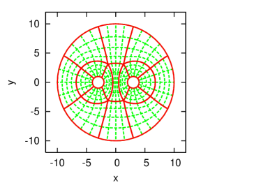
Figure 5: A cut in the equatorial plane of the imported binary black hole patch system. The outer and inner boundaries are spheres. Near the boundaries, the coordinate system is similar to spherical coordinates, i.e., there is one coordinate direction perpendicular to and two direction tangential to the boundary.

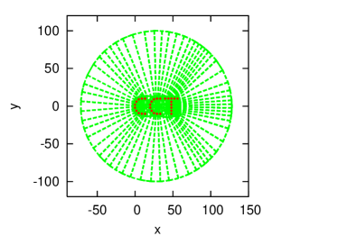
(a) whole domain

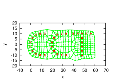
(b) region near the origin

Figure 6: A cut in the equatorial plane of the imported demonstration patch system with 30 spherical holes in arbitrary positions close to the centre. The resolution in the centre is much higher than near the outer boundary, demonstrating how to achieve the same effect as fixed mesh refinement with multiple patches.

V Tests with the scalar wave equation

We test our multi-patch infrastructure with a scalar wave equation on an arbitrary, time-independent background. Since we express the coordinate distortions via a generic three-metric, there is —from the point of view of the code— no difference between a flat and a curved spacetime. A stationary black hole background requires non-trivial lapse and shift functions, but these are desirable even for flat spacetimes: a non-zero shift makes for moving or rotating coordinate systems (implementing fictitious forces), and a non-unity lapse could be used to advance different parts of the domain with different speeds in time, which can improve time integration efficiency (although we did not use it for that purpose).

We use the notation $\alpha$ for the lapse, $\beta^{i}$ for the shift vector, $\gamma_{ij}$ for the three-metric, $\gamma^{ij}$ for its inverse, and $\gamma=\det(\gamma_{ij})$ for its determinant.

We evolve the scalar wave equation

$$\Box u = 0$$ (2)

by introducing the auxiliary variables

$$\rho = \partial_{t}u$$ (3)

$$v_{i} = D_{i}u\text{.}$$ (4)

This renders the system into a first order form, leading to the time evolution equations

$$\partial_{t}u = \rho$$ (5)

$$\partial_{t}\rho = \beta^{i}\partial_{i}\rho+\frac{\alpha}{\sqrt{\gamma}}\partial_{i}\left[\frac{\sqrt{\gamma}}{\alpha}\left(\beta^{i}\rho+\alpha^{2}H^{ij}v_{j}\right)\right]$$ (6)

$$\partial_{t}v_{i} = \partial_{i}\rho$$ (7)

with

$$H^{ij} = \gamma^{ij}-\beta^{i}\beta^{j}/\alpha^{2}\text{.}$$ (8)

If discretised with operators that satisfy summation by parts, this system is numerically stable with respect to the energy

$$E = \frac{1}{2}\int\frac{\sqrt{\gamma}}{\alpha}\left[\rho^{2}+\alpha^{2}H^{ij}v_{i}v_{j}\right]\,dV$$ (9)

for $|\beta|<\alpha$. In this case, this system is symmetric hyperbolic, and its characteristic variables and speeds are listed in Lehner et al. (2005).

We present below evolutions of the scalar wave equation on a flat background with the seven patch system and on a Kerr–Schild background with the six patch system. We compare the respective benefits of using a global or a patch-local tensor basis, and we study the behaviour of scalar waves on a Kerr–Schild background as a test problem.

V.1 Comparing global and patch-local tensor bases

We present here time evolutions of the scalar wave equation on a flat background with the seven-patch system. We compare two formulations, one based on a global, the other based on a patch-local tensor basis. We also apply a certain amount of artificial dissipation to the system, which is necessary because our formulation has non-constant coefficients. We use two different kinds of artificial dissipation, which were introduce by Kreiss and Oliger Kreiss and Oliger (1973) and by Mattsson, Svärd, and Nordström Mattsson et al. (2004), respectively.

We set the initial condition from an analytic solution of the wave equation, namely a traveling plane wave. We also impose the analytic solution as penalty boundary condition on the outer boundaries. This is in the continuum limit equivalent to imposing no boundary condition onto the outgoing characteristics and imposing the analytic solution as Dirichlet condition onto the incoming characteristics. The patch system has the outer boundary at $r=3$, and the inner, cubic patch has the extent $[-1;+1]$. We use the penalty strength $\delta=0$ at the inter-patch and at the outer boundaries. See Diener et al. (2005) for our notation for the penalty terms.

The traveling plane wave is described by

$$u(t,x_{i}) = A\,\cos\left[2\pi\left(k_{i}x^{i}+\omega t\right)\right]$$ (10)

with $\omega^{2}=\delta^{ij}k_{i}k_{j}$. We set $A=1$ and $k_{i}=[0.2,0.2,0.2]$, so that the wave length is $5/\!\sqrt{3}$. We construct the solutions for $\rho$ and $v_{i}$ from $u$ via their definitions (3) and (4), and evaluate these at $t=0$ to obtain the initial condition. The flat background has $\alpha=1$, $\beta^{i}=0$, and $\gamma_{ij}=\delta_{ij}$ in the global tensor basis; the patch-local metric is constructed from that via a coordinate transformation.

We use dissipation operators that are compatible with summation by parts (SBP) finite difference operators. Introduced by Mattsson, Svärd, and Nordström in Mattsson et al. (2004), we call them “MSN” operators. They are constructed according to

$$A_{2p}^{\mathrm{MSN}} = -\frac{\epsilon}{2^{2p}}\,h^{2p}\;\Sigma^{-1}D_{p}^{T}B_{p}D_{p}\text{,}$$ (11)

where $2p$ is the order of the interior derivative operator, $\epsilon$ is the dissipation strength, $h$ is the grid spacing, $\Sigma$ is the norm with respect to which the derivative operator satisfies SBP, $D_{p}$ is a consistent approximation of a $p$th derivative, and $B_{p}$ is a diagonal matrix. The scaling with grid spacing is in contrast to standard Kreiss–Oliger (KO) dissipation operators Kreiss and Oliger (1973), where the scaling $h^{2p-1}$ is used. Experience has shown that with the MSN scaling it is sometimes necessary to increase the dissipation strength when resolution is increased in order to maintain stability. For this reason we have implemented SBP compatible KO dissipation operators constructed according to

$$A_{2p}^{\mathrm{KO}} = -\frac{\epsilon}{2^{2p+2}}\,h^{2p+1}\;\Sigma^{-1}D_{p+1}^{T}B_{p}D_{p+1}\text{,}$$ (12)

where as before $\Sigma$ is the norm of the $2p$th order accurate SBP derivative operator. This yields a dissipation operator with KO scaling that has the same accuracy as the SBP derivative operator near the boundary (and one order higher in the interior). The price is having to use a slightly wider stencil.

We use $21$ grid points in the angular and in the radial directions. The central patch also has $21$ grid points in each direction. This is a very coarse resolution. We use the $D_{6-5}$ stencil of Diener et al. (2005), which is globally sixth order accurate, and add compatible artificial dissipation to the system of both MSN and KO type as described above. We choose a dissipation coefficient $\epsilon=3.0$. We use a transition region that is $0.3$ times the size of the patch. The overall system is then sixth order accurate.

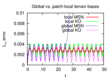
Figure 7: Comparing global and patch-local tensor bases, and Mattsson–Svärd–Nordström (MSN) and Kreiss–Oliger (KO) dissipation operators. The graphs show the $L_{\infty}$ norm of the solution error vs. time for a coarse resolution on a seven-patch system. Some artificial dissipation is necessary to stabilise the system, since it has non-constant coefficients. For this particular value of the dissipation strength $\epsilon$, using a global tensor basis is unstable with the MSN dissipation operators, but stable with the KO operators. With higher values of $\epsilon$, the system is stable for both dissipation operators.

With a patch-local tensor basis and diagonal norm operators the system is strictly stable, i.e., the numerical error is at any given resolution bounded (up to boundary terms) by a constant (see also Diener et al. (2005)), while with a global tensor basis, a small amount of artificial dissipation is required. However, since we are using restricted full norm operators for this test, dissipation is required for both the patch-local and patch-global case.

Figure 7 shows the $L_{\infty}$ norm of the solution error vs. time up to $t=50$. The discretisation using MSN dissipation is unstable for $\epsilon=3.0$ when a global tensor basis is used, but it is stable when a local tensor basis is used. Larger values of $\epsilon$ also stabilise the global tensor basis discretisation. For the KO dissipation, a dissipation strength $\epsilon=3.0$ is sufficient to stabilise both the local and global tensor basis formulations. Note that the error levels are very similar in all cases, showing that the main difference between the patch-local and patch-global tensor basis implementations is that more dissipation is necessary in order to stabilise the system.

Finally, we show a typical shape for solution errors in figure 8. This shows the solution errors in the quantity $u$ across the $+x$ block for two different resolutions. The simulation started with a Gaussian pulse as initial condition. The graph shows the errors at the time $t=25$ along the $a$ coordinate line for $b=0,\,c=0$; this coordinate line is approximately the $\phi$ coordinate line, except that it has a kink at the block interfaces. (See figure 4 for an illustration.) $b=0$ places the coordinate line into the equatorial plane, and $c=0$ chooses the centre of the block in the radial direction. The coarse block had $17\times 17\times 141$ grid points with the outer boundary at $R=15$, and the fine block had twice this resolution. The simulation was run with the $D_{6-5}$ operator, and we expect 6th order convergence. We have intentionally chosen rather coarse resolutions in the angular direction. Because the SBP stencils of the $D_{6-5}$ operator are modified on 7 grid points near each boundary, convergence at the boundary is not obvious from this graph. However, we show in Diener et al. (2005) that this system converges indeed to 6th order.

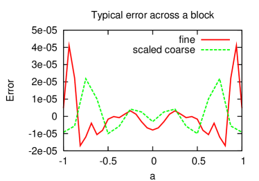
Figure 8: This figure shows typical solution error shapes across a block. It shows the error along the $a$ coordinate line of the $+x$ patch of a seven-patch system. This coordinate line corresponds to a $\phi$ coordinate line in spherical coordinates, but has a kink at the patch interface; see figure 4. This figure shows two resolutions which differ by a factor of two, and the coarse error is scaled according to 6th order convergence. The error is largest near the block boundary. Because the SBP stencils of the $D_{6-5}$ operator are modified on 7 grid points near each boundary, convergence near the boundary is not obvious from this graph. We show 6th order convergence for this case in Diener et al. (2005).

V.2 Scalar wave equation on a Kerr–Schild background

We also present time evolutions of the scalar wave equation on a Kerr–Schild (Cook, 2000, section 3.3) background with six patches, which we use to excise the singularity. We choose the mass $M=1$ and the spin $a=0.9$ for the background. We place the inner boundary at $r=1.4$ and the outer boundary at $r=201.4$.

We use as initial condition $u(0,x^{i})=0$, $v_{i}(0,x^{i})=0$, and a modulated Gaussian pulse

$$\rho(0,x^{i}) = Y_{\ell m}\,A\exp\left[-\frac{(r-R)^{2}}{W^{2}}\right]\text{,}$$ (13)

where we choose the multipole $\ell=2,\,m=2$, the amplitude $A=1$, the radius $R=20$, and the width $W=1$. We use conventions such that

$$Y_{22} = \sqrt{\frac{15}{32\pi}}\sin^{2}\theta\left(\cos^{2}\phi-\sin^{2}\phi\right)\text{.}$$ (14)

We impose $u=0$, $\rho=0$, and $v_{i}=0$ with the penalty method as outer boundary conditions. This means that this condition is imposed onto the incoming characteristic modes. Since the inner boundary is an outflow boundary, no boundary condition is imposed there. At the outer boundary, $\rho$ is indistinguishably close to zero at $t=0$ (much closer than the floating point round-off error), so that there is no noticeable discontinuity to the initial condition. We use again the penalty strength $\delta=0$ for both inter-patch and outer boundaries.

We use the patch-local tensor basis for this example. We use $21$ grid points in the angular directions and $1001$ grid points in the radial direction. We use here —for no particular reason— different discretisation parameters. It is our experience that the stability of the system does not depend on the particular choice of stencil, as long as it satisfies summation by parts Diener et al. (2005). We use here the $D_{8-4}$ stencil, which is globally fifth order accurate, and add compatible MSN artificial dissipation to the system. We choose a dissipation coefficient $\epsilon=0.2$, and we do not scale the dissipation with the grid spacing $h$. The overall system is then fifth order accurate. We use a fixed time step size $\Delta t=0.05$ with a fourth order accurate Runge–Kutta integrator.

Figure 9 shows a snapshot of the simulation at $t=92.2$. At that time, the wave pulse has traveled approximately half the distance to the outer boundary. The inter-patch boundaries are smooth, although the configuration is not axisymmetric. Figure 10 shows extracted wave forms from this simulation for the $\ell=2,\,m=2$ and for the $\ell=4,\,m=2$ modes. The $\ell=2$ mode is present in the initial condition. The $\ell=4$ mode is excited through mode–mode coupling. Its amplitude is $10^{3}$ times smaller than the $\ell=2$ mode at this time. The $\ell=4$ mode has converged at this resolution, i.e., it does not change noticeably when the resolution is changed.

We have also simulated initial data consisting of an $\ell=2,\,m=0$ mode. In this case, both the $\ell=0,\,m=0$ and the $\ell=4,\,m=0$ modes are excited through mode–mode coupling. As expected, the mode–mode coupling vanishes when the spin of the background spacetime is set to zero.

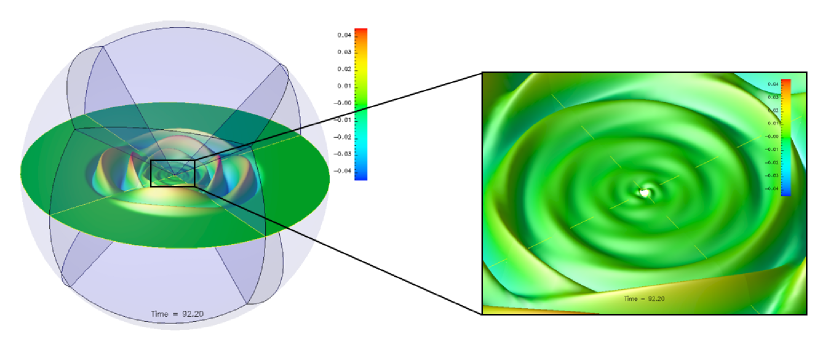
Figure 9: The patch system and the scalar wave configuration at $t=92.2$, also enlarging the region near the excision boundary inside the horizon. The background is a rotating black hole with $a=0.9$, the initial condition is an $\ell=2,\,m=2$ multipole. Note the large scale difference between the outer and the inner boundary, which is handled “naturally” and without mesh refinement. There are no artifacts visible at the inter-patch boundaries.

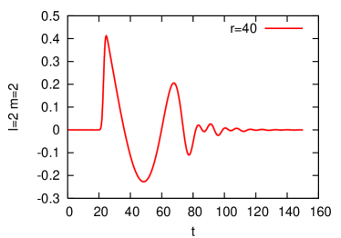
(a) $\ell=2,\,m=2$

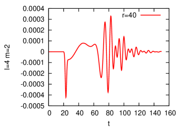
(b) $\ell=4,\,m=2$

Figure 10: The $\ell=2,\,m=2$ and the $\ell=4,\,m=2$ modes, extracted at $r=40$. The $\ell=4,\,m=2$ mode is excited through mode–mode coupling. Its amplitude is $10^{3}$ times smaller than the $\ell=2,\,m=2$ mode. All other modes with $\ell\leq 4$ are zero up to floating point round-off error.

We determine the complex quasi normal frequency $\omega=\omega_{R}+i\omega_{I}$ from the extracted wave form of the $\ell=2,\,m=2$ mode. We fit the wave seen by an observer at radius $r=5$ to a function

$$f(t) = A\sin(\omega_{R}t-\phi)\exp(\omega_{I}t)\text{.}$$ (15)

This fit is performed for the real and imaginary part of the complex frequency as well as for the amplitude $A$ and a phase $\phi$. Table 1 shows the frequencies we obtain from our simulations for the $\ell=2,\,m=2$ and $m=-2$ modes and we compare the predictions made by perturbation theory Berti et al. (2004); Berti and Kokkotas (2005). A detailed study of quasi-normal mode frequencies and excitation coefficients of scalar perturbations of Kerr black holes is in preparation Dorband et al. (2006).

For reasons of comparison between a code using the global tensor basis and one using the patch-local tensor basis, we evolved a similar physical system using both of these methods. We now choose a spin of $a=0.5$ and initial data with an $\ell=2,\,m=0$ angular dependency. The frequencies obtained by both codes, together with the predictions from perturbation theory are shown in table 1. We find that the choice of tensor basis has little influence on the accuracy of the results.

Mode			Spin	$\omega_{\mathrm{peturbation}}$			$\omega_{\mathrm{numerical}}$
$l=2$	,	$m=2$	$0.9$	$0.781638$	$-$	$0.0692893i$	$0.796527(030)$	$-$	$0.0680891(010)i$
$l=2$	,	$m=-2$	$0.9$	$0.387710$	$-$	$0.0935902i$	$0.387678(001)$	$-$	$0.0934718(100)i$
$l=2$	,	$m=0$	$0.5$	$0.491962$	$-$	$0.094630i$	$0.491824(100)$	$-$	$0.0946523(200)i$	(local)
$l=2$	,	$m=0$	$0.5$	$0.491962$	$-$	$0.094630i$	$0.492432(001)$	$-$	$0.0944723(300)i$	(global)

Table 1: Comparison of the scalar quasi normal frequencies obtained with the multi block method using a global and local tensor basis, and the values predicted by perturbative methods Berti et al. (2004); Berti and Kokkotas (2005). The given error estimates for the numerical values come from the uncertainty induced by the fitting procedure. Details about that can be found in Dorband et al. (2006).

VI Evolving the vacuum Einstein equations

We evolve the vacuum Einstein equations using the symmetric hyperbolic formulation introduced in Sarbach and Tiglio (2002). It includes as variables the three metric $g_{ij}$, the extrinsic curvature $K_{ij}$, the lapse $\alpha$, and extra variables denoted by $d_{kij}$ and $A_{i}$. When all the constraints are satisfied, these are related to the three-metric and lapse by $d_{kij}=\partial_{k}g_{ij}$ and $A_{k}=\partial_{k}\ln\alpha$. The formulation admits any of the Bona–Masso slicing conditions while still being symmetric hyperbolic. The shift has to be specified in advance as an arbitrary function of the spacetime coordinates $t$ and $x^{i}$. In the tests below, we use a time harmonic slicing condition and a time-independent shift. The characteristic modes and speeds are listed in Sarbach and Tiglio (2002).

Previous $3D$ black hole simulations using this formulation were presented in Tiglio et al. (2004), using a low order Cartesian code and cubic excision. In Sarbach and Tiglio (2005), constraint-preserving boundary conditions for this formulation were constructed; this paper then studies the well-posedness of the resulting initial-boundary value problem, and tests a numerical implementation of those boundary conditions in fully non-linear $3D$ scenarios as well, again with a Cartesian code.

After some initial (and quite lengthy) experiments with a patch-local tensor basis, we decided to use a global tensor basis instead. We find that patch-local tensor bases increase the complexity of the inter-patch boundary conditions very much, because the characteristic decomposition of the field variables needs to be combined with the tensor basis transformation at the patch boundaries. Converting the partial derivatives into the global tensor basis is trivial in comparison. In addition to that, analysing and visualising the output of a simulation is also made much easier when a global tensor basis is used.

VI.1 Robust stability test

The robust stability test in numerical relativity consists of evolving featureless initial conditions to which random noise has been added. This test was initially suggested in Szilágyi et al. (2000); Szilagyi et al. (2002) and later refined in the so-called Mexico tests Alcubierre et al. (2004b); see also app . The first stage of this test has a domain that is periodic in all directions, i.e., has a $T^{3}$ topology. The most difficult stage of the test has a spherical outer boundary through which noise is injected.

We implement the $T^{3}$ topology with a single patch, using penalty inter-patch boundary conditions to give the system a toroidal topology. We also use a six-patch topology and set the incoming modes to Minkowski on both the inner and outer boundary. The single patches have outer boundaries at $x^{i}\in[-1;+1]$, the six-patch system has the inner boundary at $r=1.9$ and the outer boundary at $r=11.9$. We use a Minkowski spacetime as background and add random noise with an amplitude of $10^{-8}$ to all variables. Since the Minkowski spacetime has no intrinsic scale, this amplitude should be compared to our floating point accuracy of approximately $10^{-16}$. Terms that are quadratic in the noise amplitude have then the same order of magnitude as floating point inaccuracies.

In the runs shown below, we choose the penalty parameter $\delta=0.5$. We discretise the domain with $21^{3}$, $41^{3}$, and $81^{3}$ grid points per patch. We use the $D_{8-4}$ derivative operator and its associated KO dissipation with a parameter $\epsilon=0.5$. We also use an adaptive Runge–Kutta time integrator. For comparison, we also show results using a six-patch system with the $D_{6-5}$ operator, using the same dissipation parameter.

Figure 11 shows the $L_{\infty}$ norm of the Hamiltonian constraint as a function of time. The constraints remain essentially constant. Note that the constraints do not converge to zero with increasing resolution, since the random data are different for each run and do not have a continuum limit.

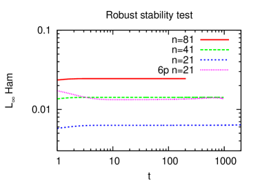
Figure 11: Robust stability test for the Einstein equations. This graph compares three different resolution of a single patch and the six-patch system. Random noise is initially added to all variables. At late times, the Hamiltonian constraint does not grow with time; the system is strictly stable. The two runs marked $n=81$ and $6p\;n=21$ have the highest resolutions; we aborted them before they reached $t=2000$, which corresponds to $1000$ crossing times for the single patch.

VI.2 One-dimensional gauge wave

One of the most difficult of the Mexico tests Alcubierre et al. (2004b); app is the gauge wave test. This is a one-dimensional non-linear gauge wave, i.e., flat space in a non-trivial coordinate system. This setup lives in a $T^{1}$ domain, i.e., it has again periodic boundaries, which we implement either as manifestly periodic boundary conditions or as penalty inter-patch boundary conditions. We use the slightly modified gauge wave which has the line element

$$ds^{2} = -H\,dt^{2}+H\,dx^{2}+dy^{2}+dz^{2}$$ (16)

with

$$H = \exp\left[A\sin\left(\frac{2\pi(x-t)}{L}\right)\right]\text{.}$$ (17)

We choose the wave length $L$ to be the size of our domain, and set the amplitude $A$ to $0.5$.

Our domain is one-dimensional with $x\in[-1;+1]$. Different from Alcubierre et al. (2004b), we place grid points onto the boundaries. We use either $41$ or $81$ grid points. Figure 12 compares the shape of the wave form at late times to its initial shape. Our system is stable and very accurate even after $1000$ crossing times when we use manifestly periodic boundary conditions. When we impose periodicity via penalties, the system is less accurate, and these inaccuracies lead to a drift which finally leads to a negative $g_{11}$, which is unstable. With $81$ grid points per wave length, however, our system is both stable and very accurate after $1000$ crossing times even with penalty boundaries.

Standard lore says that a second order discretisation requires one to use at least 20 grid points per wave length. This would seem to make it excessive to use 81 grid points per wave length with our fifth order scheme. However, this is not so. According to Kreiss and Oliger Kreiss and Oliger (1973), using 20 grid points per wave length introduces a 10% error for each crossing time, making it impossible to evolve meaningfully for 1000 crossing times. Achieving a 1% error after 1000 crossing time requires about 2000 grid points for a second order scheme, and approximately 73 grid points for a fourth order scheme. Given these numbers, using 81 grid points for our fifth order scheme is appropriate.

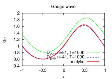
(a) Manifestly periodic

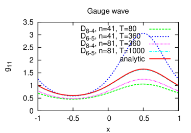
(b) Periodic via penalties

Figure 12: Results for the gauge wave test case, comparing differencing operators and resolutions. With manifestly periodic boundaries, the system is both stable and highly accurate after $1000$ crossing times. With periodicity imposed via penalty boundary conditions, the system is less accurate, and lower resolutions are finally unstable after $g_{11}$ becomes negative. However, with sufficient resolution and high order derivatives, our system is still highly accurate after $1000$ crossing times.

VI.3 Weak gravitational waves

We now consider perturbations of a flat spacetime, using the Regge–Wheeler (RW) perturbation theory Regge and Wheeler (1957) to construct an exact solution to the linearised constraints of Einstein’s equations, which we evolve with the fully non-linear equations. We linearise about the Minkowski spacetime, i.e., we choose a background spacetime with the ADM mass $M=0$.

For simplicity we consider an $\ell=2,\,m=0$ odd parity perturbation. The resulting metric in the Regge–Wheeler gauge and in spherical coordinates is

$$ds^{2} = -dt^{2}+dr^{2}+r^{2}(d\theta^{2}+\sin^{2}\theta\,d\phi^{2})$$

$${}-6\,\delta\,r\dot{\Psi}\,\sin^{2}\theta\,\cos\theta\,dr\,d\phi$$

$${}-6\,\delta(\Psi+r\Psi^{\prime})\sin^{2}\theta\,\cos\theta\,dt\,d\phi$$

where a prime denotes derivative with respect to $r$, and where $\delta$ is a parameter that determines the “strength” of the perturbation (not to be confused with the penalty term, for which we use the same symbol). This metric satisfies the linearised constraints for any functions $\Psi(t=0,r)$ and $\dot{\Psi}(t=0,r)$, and satisfies all the linearised Einstein equations if $\Psi$ satisfies the Regge-Wheeler equation

$$\ddot{\Psi} = \Psi^{\prime\prime}-\frac{6}{r^{2}}\Psi\text{.}$$ (19)

It is simple to construct a purely outgoing, exact solution to the previous equation:

$$\Psi(u,r) = \frac{d^{2}F}{du^{2}}-\frac{3}{r}\frac{dF}{du}+\frac{3}{r^{2}}F$$ (20)

where $F(u)$ is an arbitrary function of $u=r-t$. The above metric is very similar to the one in Teukolsky (1982), except that ours is in the Regge–Wheeler gauge.

However, we use a different coordinate condition for our evolutions. We construct from the previous metric initial conditions in Cartesian coordinates for $g_{ij}$, $K_{ij}$, and $d_{kij}$. We set the initial lapse to one and evolve it through the time harmonic slicing condition, and set the shift to zero at all times.

We now want to check at what point non-linear effects begin to have an effect on the constraints. That is, we want to find out what resolutions are required to see that the full, non-linear constraints do not actually converge to zero. As initial condition for the function $\Psi$ and its time derivative we choose

$$\Psi(t=0,r) = A\exp\left(-\frac{(r-r_{0})^{2}}{\sigma^{2}}\right)$$ (21)

$$\dot{\Psi}(t=0,r) = -2\,\frac{(r-r_{0})}{\sigma^{2}}\,B\exp\left(-\frac{(r-r_{0})^{2}}{\sigma^{2}}\right)\text{.}$$ (22)

The non-linear constraint violations should have an approximate quadratic dependence on the amplitude parameter (called $A$ below). Figure 13 quantifies this violation. It displays the $L_{2}$ and $L_{\infty}$ norms of the non-linear Hamiltonian constraint, measured in local coordinates, for different families of initial conditions as a function of resolution. We use the seven-patch system described in section IV with the outer boundary at $r=6$, while the inner, cubic patch has an extent of $\pm 1$. The initial condition parameters are $B=-A$, $\sigma=0.6$, and $r_{0}=3$, with amplitudes $\delta=10^{-1},10^{-2},10^{-3},10^{-4}$. We use the $D_{6-5}$ derivative with $N^{3}$ grid points on each patch for $N=21,41,81,161$. At the highest resolution, the numerical constraints reach their non-zero continuum values. This highest resolution corresponds to $24$ grid points per $\sigma$ in the radial direction. This number is comparable to the coarsest resolutions that we use in the simulations presented below. This means that those simulations use constraint-violating initial conditions, and cannot expect the constraints to decrease with increasing resolution.

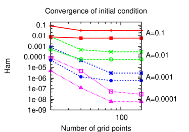
Figure 13: Norms of the Hamiltonian constraint for initial conditions with different amplitudes as a function of the number of grid points on each patch in each direction. For each initial amplitude we show both the $L_{2}$ and the $L_{\infty}$ norm. Since the initial conditions only satisfy the linearised constraints, we clearly see the non-linear constraint violation at the highest resolutions.

The non-linear constraint violation should be approximately a quadratic function of the amplitude of the perturbation $\delta$, at least for small values of $\delta$. Figure 14 shows that this is indeed the case. It displays the Hamiltonian constraint violation in the $L_{2}$ norm for the highest resolution of the previous figure as a function of the amplitude $\delta$. The measured slope is $2.0002$. Figure 15 shows a sample evolution of this odd parity initial condition family, using the six-patch geometry.

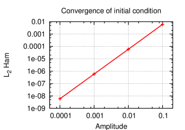
Figure 14: Hamiltonian constraint violation in the $L_{2}$ norm as a function of the amplitude of the perturbation for the highest resolution. This shows the expected quadratic dependence on the amplitude.

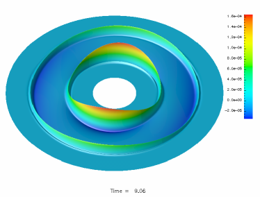
Figure 15: Evolution of weak gravitational waves. This shows the component $K_{xx}$ of the extrinsic curvature in the equatorial plane at $t=9.06$. The gravitational wave packet started as a spherical shell approximately in the middle between the inner and outer boundaries, and has then split into two packets which travel outwards and inwards, respectively.

In order to evaluate the accuracy of our code we now choose an initial condition corresponding to an exact solution of the outgoing type described above. We do so by choosing

$$F(u) = \exp\left(-\frac{(r-r_{0})^{2}}{\sigma^{2}}\right)\text{.}$$ (23)

In these evolutions the parameters that determine the initial condition are $\sigma=1$, $r_{0}=30$, and amplitude $\delta=10^{-3}$, with inner and outer boundaries at $r=10$ and $r=60$, respectively.

We extract the wave forms from the numerical results by calculating the Regge–Wheeler function at each grid point. We then average over one radial shell. There is no need for interpolating to a sphere, which simplifies the extraction procedure greatly, and probably also improves its accuracy. Figure 16 shows the numerically extracted $\Psi_{e}$ at $r=40$, and compared to its exact value $\Psi$, for an evolution using the $D_{8-4}$ derivative, with the dissipation parameter $\epsilon=0.05$. We used two resolutions with $16\times 16\times 1001$ and $22\times 22\times 1401$ grid points on each patch. The agreement is excellent.

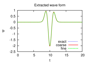
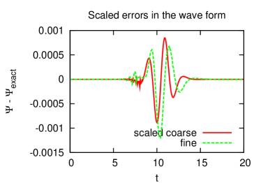
Figure 16: The upper panel shows the Regge–Wheeler function $\Psi$ vs. time, comparing the numerical and the exact solution at $r=40$. The agreement is excellent, especially for a three-dimensional, fully nonlinear code. The lower panel shows the scaled differences to the exact solution for two resolutions with $16\times 16\times 1001$ and $22\times 22\times 1401$ grid points. This demonstrates fifth order convergence, as should be the case for the $D_{8-4}$ operator.

VII Conclusions

We have motivated the use of multi-patch systems in general relativity, and have described a generic infrastructure for multi-patch time evolutions. Their main advantages are smooth boundaries and constant angular resolution, which makes them very efficient for representing systems requiring high resolution in the centre and having a radiative zone far away. They may even render fixed mesh refinement unnecessary in many cases.

We use the penalty method for inter-patch boundary conditions. It would equally be possible to use e.g. interpolation between the patches. A direct comparison of these different approaches would be very interesting. Our evolution systems are first order symmetric hyperbolic, but second order systems could be used as well. We use this infrastructure with high-order finite differencing operators, but other discretisations such as e.g. pseudo-spectral collocation methods can also be used. Our infrastructure is based on Cactus and Carpet and runs efficiently in parallel.

We have discussed the relative advantages of using global and patch-local tensor bases, and we have compared the accuracy and stability of both approaches. We suggest that using a global basis is substantially more convenient, both in the implementation of the code and in the post-processing of the generated output.

We have tested this infrastructure with a scalar wave equation on a fixed, stationary background, and with a symmetric hyperbolic formulation of the Einstein equations. We have shown that our multi-patch system with penalty boundary conditions is robustly stable and can also very accurately reproduce the nonlinear gauge wave of the Apples with Apples tests, which has been the most difficult of these tests for other codes.

Finally, we have simulated three-dimensional weak gravitational waves in three dimensions, using the same nonlinear code, and have accurately extracted the gravitational radiation. The latter is made especially simple since the wave extraction spheres are aligned with the numerical grid.

We believe that multi-patch systems, which provide smooth boundaries, will be an essential ingredient for discretising well-posed initial boundary value problems.