The standard cosmological model posits a spatially flat universe of infinite extent. However, no observation, even in principle, could verify that the matter extends to infinity. In this work we model the universe as a finite spherical ball of dust and dark energy, and obtain a lower limit estimate of its mass and present size: the mass is at least $5\times 10^{23}M_{\odot}$ and the present radius is at least 50 Gly. If we are not too far from the dust-ball edge we might expect to see a cold spot in the cosmic microwave background, and there might be suppression of the low multipoles in the angular power spectrum. Thus the model may be testable, at least in principle. We also obtain and discuss the geometry exterior to the dust ball; it is Schwarzschild-de Sitter with a naked singularity, and provides an interesting picture of cosmogenesis. Finally we briefly sketch how radiation and inflation eras may be incorporated into the model.

1 Introduction

The standard or “concordance” model of the present universe has been very successful in that it is consistent with a wide and diverse array of cosmological data. The model posits a spatially flat ($k=0$) Friedmann-Robertson-Walker (FRW) universe of infinite extent, filled with dark energy, well described by a cosmological constant, and pressureless cold dark matter or “dust.” Despite the phenomenological success of the model, our present ignorance of the physical nature of both the dark energy and dark matter should prevent us from being complacent.

The infinite extent of the standard model is at the very least a problematic feature since it cannot be confirmed by experiment, even in principle. One might be tempted to place it among the other theoretical infinities that are presently tolerated in physics, such as those of quantum field theory. In this work, we take a different approach and simply drop the assumption that the material contents of the universe go on forever. A large but finite universe (say, millions of Hubble distances) should certainly be observationally indistinguishable from one of infinite extent, at least for an observer who is not too near the edge (figure 1).

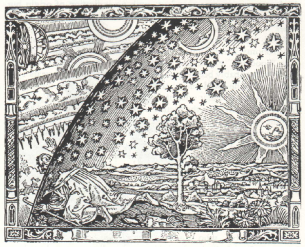
Figure 1: The medieval view of a finite universe [woodcut by an unknown artist, first published by Camille Flammarion in L’Atmosphere: Météorologie Populaire (Paris, 1888), p. 163]

Indeed, it seems obvious that we can only hope to place a lower limit on the universe’s spatial extent.

The model of the universe that we develop below is consistent with the same observational data that support the standard model in which the matter has an infinite extent; it is a spherical dust ball surrounded by an empty exterior space (figure 2). Both regions contain dark energy, represented by a cosmological constant. The dust ball is taken to have a standard FRW geometry. While this dust ball is of finite extent, the exterior space has no boundary. The geometry of the exterior is uniquely determined by that of the dust ball, and is described by a metric first found by Kottler. This is often called a Schwarzschild-de Sitter geometry because its metric approaches the Schwarzschild metric for small radii and the static de Sitter metric for large radii. The exterior has some remarkable features, prime among which is that it harbors a naked singularity that fills all of 3-space before the big bang. However, consideration of the earlier inflationary and radiation-dominated eras leads us to believe that this singularity should probably be viewed as a phenomenological representation for a small region of very heavy vacuum.

We note that this dust-ball universe is effectively a finite or truncated version of the standard $\Lambda$CDM model, and should not be confused with finite but topologically non-trivial models such as the Poincaré dodecahedron.

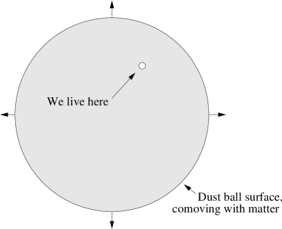
Figure 2: The general features of our finite universe model. The dust ball consists of cold matter and dark energy, and expands into an empty, time-independent exterior whose nature is to be determined.

The paper is organized as follows. In section 2 we describe the geometry of the dust ball and obtain lower limits on its total mass and size. These limits are determined by the fact that we do not at present see any obvious edge; the mass limit is about $5\times 10^{23}M_{\odot}$ and the size limit is about 50 Gly. Section 3 contains comments on the possibility of testing the model; specifically, if we are close enough to the edge, there may be a “cold spot” detectable in the cosmic microwave background (CMB). In section 4 we obtain the metric for the exterior, which is completely determined by that of the dust ball and the demands of spherical symmetry and time independence. This is most conveniently done in Painlevé-Gullstrand (PG) coordinates, but we also give the exterior metric in FRW-like and Schwarzschild coordinates. In section 5 we transform the metric for the exterior to conformal form, discussing the nature of the exterior geometry and the picture of cosmogenesis that it suggests, wherein the material contents of our universe explode from a 3-space-filling singularity. The emphasis of this work is on the present cosmic era, but in section 6 we briefly sketch an approach to the early universe, incorporating simple inflationary and radiation-dominated eras into the model; one amusing result is that the singularity noted above is replaced by a region of heavy vacuum. Much further work could be done on the early finite universe.

We emphasize that the discussion of the dust ball and the mass and size limits in sections 2 and 3 are well-founded extensions of the general-relativistic standard cosmological model, and are self-contained. The discussions of the exterior, the early universe and cosmogenesis in later sections are more speculative. Altogether, we use six different coordinate systems in obtaining our results; this is an amusingly large number but probably not a record in the field.

2 The universe in the dust ball

We will assume that the standard cosmological model (defined here as flat $\Lambda$CDM) is correct in its essential features. Thus we take the interior of the dust ball in figure 2 to have a spatially flat FRW metric, and to be dominated by dark energy, represented by the cosmological constant, and dust-like matter. However, we truncate the matter at a comoving radius $u_{\scriptscriptstyle db}$ to form a finite sphere, as shown in figure 2. The main result of this section will be a lower limit on the mass and size of the dust ball. We work in FRW coordinates with both cosmic and conformal time coordinates.

The metric of the dust ball in FRW coordinates is given in standard form (with $c=1$) by

$$ds^{2}=dt^{2}-a^{2}(t)[\,du^{2}+u^{2}(d\theta^{2}+\sin^{2}\!\theta\,d\phi^{2}\,)]\;,\;\;\;u<u_{\scriptscriptstyle db}\;.$$ (1)

We use a dimensionless radial coordinate $u$ so that the scale function $a(t)$ has the dimension of a distance; $u_{\scriptscriptstyle db}$ is the comoving radius of the dust ball. The scale function must obey the Friedmann equation, which results from the Einstein field equations for the FRW metric, and reads

$$\dot{a}^{2}=\frac{{\cal C}}{a}+\frac{a^{2}}{R_{d}^{\,2}}\;.$$ (2)

Here ${\cal C}$ is a dimensionless constant of integration, and $R_{d}$ is the de Sitter radius, which is related to the cosmological constant by $R_{d}=\sqrt{3/\Lambda}$ and equal to about 16 Gly in the standard $\Lambda$CDM model. The solution appropriate to the present era is [1]

$$a(t)=({\cal C}R_{d}^{\,2})^{1/3}\sinh^{2/3}(3t/2R_{d})\;,$$ (3)

and the present time is about 14 Gyr.

To obtain a lower limit on the mass and size of the dust ball, we note that no edge has been seen. Thus our past light cone must lie entirely inside the dust ball. Analysis of the past light cone is most clearly done using conformal time, wherein the metric is proportional to the Lorentz metric and the light cone is the same 45^∘ region as in special relativity. Conformal time is defined by

$$d\eta=dt/a(t)\;,$$ (4)

in terms of which the metric becomes

$$ds^{2}=a^{2}(t)[\,d\eta^{2}-du^{2}-u^{2}(d\theta^{2}+\sin^{2}\!\theta\,d\phi^{2}\,)]\;,\;\;\;u<u_{\scriptscriptstyle db}\;.$$ (5)

The solution of eq. (4) is

$$\eta=\frac{2}{3}\left(\frac{R_{d}}{{\cal C}}\right)^{\!\!\!1/3}\!\!{\cal G}\!\left(\frac{3t}{2R_{d}}\right)\;,\;\;\;{\cal G}\!\left(\frac{3t}{2R_{d}}\right)\equiv\int_{0}^{\,3t/2R_{d}}\!\!\frac{dx}{\sinh^{2/3}(x)}\;.$$ (6)

We have here chosen the constant of integration so that $t=0$ corresponds to $\eta=0$. The function ${\cal G}$ may be obtained numerically and is plotted in figure 3.

Figure 3: Plot of the function ${\cal G}(x)=\int_{0}^{x}\sinh^{-2/3}(x^{\prime})\,dx^{\prime}$.

In particular, for the present time its value is about 3.2, so

$$\eta_{\,0}=\frac{2}{3}\left(\frac{R_{d}}{{\cal C}}\right)^{\!\!\!1/3}\!\!3.2\;,\;\;\;t_{0}=\mbox{14 Gyr}\;.$$ (7)

For the infinite future, ${\cal G}$ may be calculated exactly in terms of gamma functions, with the result

$${\cal G}(\infty)=\frac{\Gamma(1/6)\,\Gamma(1/3)}{2\Gamma(1/2)}=4.2\;,\;\;\;\eta_{\,\infty}=\frac{2}{3}\left(\frac{R_{d}}{{\cal C}}\right)^{\!\!1/3}\!\!\!\!4.2\;,\;\;\;t=\infty\;.$$ (8)

We now require that our past light cone lie entirely inside the dust ball, as shown in figure 4. It follows that

$$\eta_{\,0}+fu_{\scriptscriptstyle db}\leqslant u_{\scriptscriptstyle db}\;,$$ (9)

where $f$ is our fractional displacement from the center of the dust ball. Eqs. (7) and (9) together imply a limit on the radius of

$$\frac{\eta_{\,0}}{(1-f)}=\frac{2}{3}\left(\frac{R_{d}}{{\cal C}}\right)^{\!\!1/3}\frac{3.2}{(1-f)}\leqslant u_{\scriptscriptstyle db}\;.$$ (10)

Eq. (10) involves the physically unobservable quantities ${\cal C}$ and $u_{\scriptscriptstyle db}$; we prefer to express the inequality in terms of physical quantities. To do so, we first relate the integration constant ${\cal C}$ to the matter density using the $0,0$ component of the field equations, which is

$$8\pi G\rho=-\Lambda+3(\dot{a}^{2}/a^{2})\;.$$ (11)

Comparison of this with the Friedmann equation (2) gives ${\cal C}$ as

$${\cal C}=(8\pi G/3)\rho a^{3}\;.$$ (12)

Eq. (12) allows us to calculate the total dust mass and express it in terms of ${\cal C}$. Specifically, we calculate twice the geometric mass of the dust ball as

$$2m_{u}=2GM_{u}=(8\pi G/3)\rho\,(au_{\scriptscriptstyle db})^{3}={\cal C}u_{\scriptscriptstyle db}^{3}\;,\;\;\;{\cal C}=2m_{u}/u_{\scriptscriptstyle db}^{3}\;.$$ (13)

We will verify later that $2m_{u}$ plays the role of the Schwarzschild radius of the dust ball, as viewed from the exterior. Substituting eq. (13) into the constraint (10), we obtain the following limit on the dust ball’s Schwarzschild radius in terms of the de Sitter radius:

$$\frac{2}{3}\left(\frac{R_{d}}{2m_{u}}\right)^{\!\!\!1/3}\!\!\frac{3.2}{(1-f)}\leqslant 1\;,\;\;\;2m_{u}\geqslant\left(\frac{2}{3}\,\frac{3.2}{(1-f)}\right)^{\!\!3}\!R_{d}\;.$$ (14)

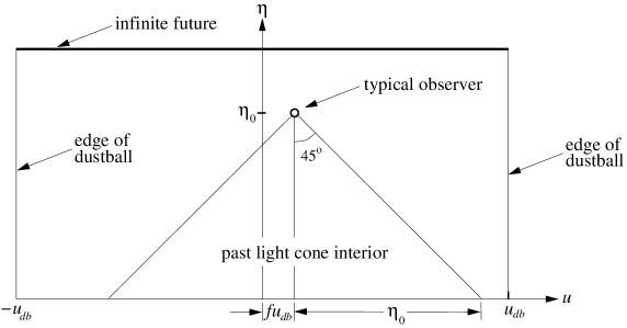
Figure 4: A cut through the conformal FRW coordinate system, showing the observer’s position and past light cone inside the dust ball.

One reasonable way to select a value for the parameter $f$ is to assume that we are at a median position inside the dust ball; specifically, that half the volume of the dust ball lies inside our radial position and half outside. This “Copernican” assumption implies that $f=(1/2)^{1/3}$, for which eq. (14) gives

$$2m_{u}\geqslant 1100R_{d}=18,000\mbox{ Gly}\;\;\;\;\;\;\mbox{ (median position)}\;.$$ (15)

Alternatively, we may be more conservative and assume only that our position lies outside the central 5% of the dust-ball volume. That is, with 95% confidence we may say that $f\geqslant(.05)^{1/3}$, which gives

$$2m_{u}\geqslant 39R_{d}=620\mbox{ Gly}\;\;\;\;\;\;\mbox{ (95\% confidence level)}\;.$$ (16)

The most conservative bound possible, of course, occurs for $f=0$, in which case

$$2m_{u}\geqslant 9.7R_{d}=160\mbox{ Gly}\;\;\;\;\;\;\mbox{ (lowest bound)}\;.$$ (17)

Since the Sun has a Schwarzschild radius of 2.9 km$=1.0\times 10^{-5}$ ls, eq. (17) translates into a lower bound on the mass of the universe in solar units of

$$M_{u}\geqslant 5.1\times 10^{23}M_{\odot}\;,$$ (18)

where $R_{d}=16$ Gly as before.

A lower bound on the present physical radius of the dust ball may be obtained from eqs. (3) and (10) with $f=0$ as

$$u_{\scriptscriptstyle db}\,a(t) \geqslant \frac{2}{3}\left(\frac{R_{d}}{{\cal C}}\right)^{\!\!1/3}\!\!\frac{3.2}{(1-f)}\,({\cal C}R_{d}^{\,2})^{1/3}\sinh^{2/3}(3t/2R_{d})$$ (19)

$$= \left[\frac{2}{3}\,\frac{3.2}{(1-f)}\sinh^{2/3}(3t/2R_{d})\right]\!R_{d}\geqslant 3.1R_{d}=49\mbox{ Gly}\;.$$

As expected, this lower limit is considerably larger than the present Hubble distance of about 14 Gly. Eqs. (18) and (19) are very conservative; higher bounds would obviously result from using the median assumption (15) or the 95% confidence-level assumption (16).

3 Observational implications

The scenario described above becomes experimentally testable if the size of the dust ball ($au_{\scriptscriptstyle db}$) is not too large or if we are sufficiently near its edge. In this case, the edge of our observable universe, which we identify with the surface of last scattering, may be near the edge of the dust ball. It is likely that the CMB temperature would decrease to zero (or a very low value) in some unknown way across a relatively thin shell (of characteristic width $\varepsilon$) around the dust ball, which would produce a cold spot in the CMB. The situation is depicted in figure 5, which might be compared with figure 2.

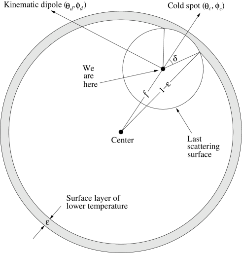
Figure 5: Geometry of the finite dust-ball universe. Distances are expressed as fractions of the dust-ball radius $u_{\scriptscriptstyle db}$. The last scattering surface may protrude into the surface layer, thereby producing a cold spot in the CMB.

After the removal of the galactic and other non-cosmological foregrounds, the CMB temperature may be written in the form

$$T=T_{0}+T_{1}+T_{2+}+T_{cs}\;,$$ (20)

where

$$T_{0} = 2.73\mbox{ K}\;\;\;\;\;\;\mbox{(monopole)}$$

$$T_{1} = T_{0}\,v_{d}\cos\theta_{d}={\cal O}(10^{-3}\mbox{K})\;\;\;\;\;\;\mbox{(kinematic dipole)}$$

$$T_{2+} = {\cal O}(10^{-5}\mbox{K})\;\;\;\;\;\;\mbox{(higher-order multipoles)}$$

$$T_{cs} = \mbox{ ?}\;\;\;\;\;\;\mbox{(cold spot)}\;.$$

Here the Sun moves at speed $v_{d}$ in the direction $(\theta_{d},\phi_{d})$ with respect to the CMB. The term $T_{2+}$ contains the usual Harrison-Zeldovich spectrum of higher-order temperature fluctuations detected by, for example, the WMAP satellite, and $T_{cs}$ is the cold spot we wish to discuss.

Assuming that the cold spot is not aligned with the Doppler dipole, the fact that it has not already made itself obvious in CMB maps implies that its magnitude is less than that of the dipole, $|T_{cs}|\lesssim 10^{-3}$K. Moreover, if $|T_{cs}|\ll 10^{-5}$K, then it is probably not possible to see the effect on the CMB. The interesting situation is therefore that in which $|T_{cs}|$ lies between approximately $10^{-6}$ K and $10^{-3}$ K.

The cold spot temperature, a function $T_{cs}(\phi,\theta)$ of angular position, will also depend on the characteristic angular width $\delta$, our fractional distance $f$ from the center of the dust ball, and the relative size $\varepsilon$ of the region of temperature decrease. The angular width has an upper limit that occurs when our line of sight just reaches the empty exterior; it is given by

$$f^{2}+(1-f)^{2}-2f(1-f)\cos(\pi-\delta)=(1-\varepsilon)^{2}\;\;\;\;\;\;\mbox{(upper limit on $\delta$)}\;,$$ (21)

or, assuming that $\varepsilon\ll 1$,

$$\delta^{2}\leqslant 2\varepsilon/f(1-f)\;\;\;\;\;\;\mbox{(approximate upper limit on $\delta$)}\;.$$ (22)

A lower limit occurs when our line of sight just reaches the shell of decreasing temperature, and is of course $\delta=0$.

A simple and reasonable choice for a parametric cold spot function is the Gaussian distribution:

$$T_{cs}=-T_{cs0}\exp(-\Delta\theta^{2}/2\delta^{2})\;,$$ (23)

where $\Delta\theta$ is angular distance from the center of the cold spot. As discussed above, we take the magnitude $T_{cs0}$ of the cold spot to lie between $10^{-6}$K and $10^{-3}$K in cases of interest. The most direct approach to testing the finite-universe idea would be to fit eq. (20) to the CMB temperature data after cleaning the latter of foreground contamination — but not correcting for the kinematic dipole, which would in general interfere with the desired cold spot signal. In principle the fit (not including the higher-order fluctuations) would involve seven parameters: the magnitude and angular direction of the Doppler dipole ($v_{d},\theta_{d},\phi_{d}$) and the magnitude, width and angular direction of the cold spot ($T_{cs0},\delta,\theta_{c},\phi_{c}$).

More sophisticated search techniques have recently led to several claims of non-Gaussianity in the WMAP data [2, 3, 4, 5], parts of which are likely local in origin since they exhibit correlations with the ecliptic plane [6, 7, 8, 9, 10, 11, 12] and the diffuse $\gamma$-ray background as measured by the EGRET satellite [13]. Of special interest for our purposes is a growing body of statistical analysis suggesting that the WMAP 1-year data is nearly Gaussian — but for a single cold spot in the direction $(l,b)=(209^{\circ},-57^{\circ})$ that is well-fit by a Gaussian function of width $\delta=4^{\circ}$ and magnitude $T_{cs0}=73~{}\mu$K [14, 15, 16, 18]. This spot appears to be incompatible with either a thermal Sunyaev-Zeldovich effect or incomplete galactic foreground subtraction [19], leading theorists to speculate on such possible causes as large-scale inhomogeneity [20], Bianchi-type models with nonzero shear or rotation [21] and homogeneous, spherically-symmetric local voids [17]. Alternatively, we note that the reported value of $T_{cs0}$ lies within the range of interest for a universe that is standard in every way except that it is of finite, rather than infinite spatial extent . Accepting the reported value of $\delta$ and adopting the median or most likely value of $f=(1/2)^{1/3}$, we find from eq. (22) that the fractional edge thickness $\varepsilon$ in such a model is less than about $4.0\times 10^{-4}$.

Some cosmologists believe there is independent evidence for a closed and finite universe in the suppression (relative to the dipole) of the lowest-order multipoles in the power spectrum of CMB fluctuations [22, 23]. In particular, the quadrupole moment is about seven times weaker than expected on the basis of a flat $\Lambda$CDM model, and the octupole is only about 72% of its expected value [24]. While this suppression may be an artifact of cosmic variance, it can also arise if the universe simply does not have enough room for the longest-wavelength fluctuations. Non-trivial topology is not required for such suppression; it is only necessary that the initial fluctuation spectrum truncate at around the curvature scale of the universe [22]. Such an effect might allow one to perform an independent experimental test of the finite-universe model by re-computing the low-order CMB multipole moments $C_{\ell}$, using eq. (20) and standard techniques. It would be of considerable interest to see if our finite-universe model produced the observed suppression of low-order multipoles; this would involve the thermodynamcs of the early universe, which we will briefly discuss in section 6.

4 Outside the dust ball

The dust ball in our model universe has a spatially flat FRW metric, and according to section 2 its Schwarzschild radius is much larger than its de Sitter radius, $2m_{u}/R_{d}\gg 1$. To study the exterior, we naturally assume that its metric is spherically symmetric and time-independent. Of course, it must also match the dust ball on its surface. These assumptions uniquely determine the exterior geometry.

The spherical symmetry and time independence of the exterior lead to a standard Schwarzschild form for the metric, which we write in the form

$$ds^{2}=(1-v^{2})\,dt_{s}^{2}-\frac{dr^{2}}{(1-w^{2})}-r^{2}d\Omega^{\,2}\;,\;\;\;\;\;\;v=v(r),w=w(r)\;.$$ (24)

The mathematical problem is to match this to the metric of the dust ball at the surface, and thereby obtain the functions $v(r)$ and $w(r)$. This is particularly easy in Painlevé-Gullstrand (PG) coordinates, which use both the FRW cosmic time and the Schwarzschild radial marker, thereby interpolating effectively between the two sets of coordinates. We therefore transform both the dust-ball metric (1), with eq. (3), and the exterior metric (24) to PG coordinates. For the exterior we introduce the PG time $t$ as

$$t_{s}=t-{\cal P}(r)\;,$$ (25)

and obtain the metric in PG form [25, 26]:

$$ds^{2}=(1-v^{2})\,dt^{2}\pm 2v\,dr\,dt-dr^{2}-r^{2}d\Omega^{\,2}\;,$$ (26)

provided that we choose $w(r)=v(r)$ and require that ${\cal P}$ satisfy

$${\cal P}^{\prime}=\pm\frac{v}{1-v^{2}}\;.$$ (27)

For our purposes, it is not necessary to solve explicitly for ${\cal P}$. For the dust ball, we transform the dimensionless FRW radial coordinate to a new radial coordinate by

$$r=a(t)u$$ (28)

and obtain

$$ds^{2}=[1-(r\dot{a}/a)^{2}]\,dt^{2}+2\,(r\dot{a}/a)\,drdt-dr^{2}-r^{2}d\Omega^{\,2}\;,$$ (29)

where $a(t)$ is given explicitly for the present era in eq. (3), and the overdot indicates differentiation with respect to time $t$. Both the exterior metric (26) and dust-ball metric (29) now have the same form, which makes the PG coordinates very convenient. It only remains to match the functions $v$ and $r\dot{a}/a$ at the dust-ball surface.

To determine the function $v(r)$ of the exterior, we first demand that the motion of the dust-ball surface, which we denote by $r_{s}(t)$, be consistent with the comoving interior material at the surface, or

$$r_{s}(t)=u_{\scriptscriptstyle db}a(t)\;\;\;\;\;\;\mbox{(surface)}\;.$$ (30)

We also demand that the dust-ball and exterior metrics match at the surface, or

$$v=r_{s}(t)\dot{a}/a=u_{\scriptscriptstyle db}\dot{a}\;\;\;\;\;\;\mbox{(surface)}\;.$$ (31)

We substitute for $\dot{a}$ from eq. (3) to obtain eq. (31) in the form:

$$v=u_{\scriptscriptstyle db}\left(\frac{{\cal C}}{R_{d}}\right)^{\!\!\!1/3}\!\!\!\frac{\cosh(3t/2R_{d})}{\sinh^{1/3}(3t/2R_{d})}\;\;\;\;\;\;\mbox{(surface)}\;.$$ (32)

Next, using eqs. (3) and (30), we relate $t$ to $r_{s}$ on the surface:

$$\sinh(3t/2R_{d})=\frac{r_{s}^{3/2}}{u_{\scriptscriptstyle db}^{3/2}(R_{d}^{\,2}\,{\cal C})^{1/2}}\;\;\;\;\;\;\mbox{(surface)}\;.$$ (33)

Finally, we substitute from eq. (33) into eq. (32) to obtain

$$v=\sqrt{\frac{{\cal C}\,u_{\scriptscriptstyle db}^{3}}{r}+\frac{r^{2}}{R_{d}^{\,2}}}=\sqrt{\frac{2m_{u}}{r}+\frac{r^{2}}{R_{d}^{\,2}}}\;.$$ (34)

Since $v$ is a function of only $r$, Eq. (34) must hold throughout the exterior and not just on the surface of the dust ball. We have therefore dropped the subscript on $r$; this gives the metric of the exterior. Explicitly, in PG coordinates,

$$ds^{2}=\left(1-\frac{2m_{u}}{r}-\frac{r^{2}}{R_{d}^{\,2}}\right)\,dt^{2}+2\sqrt{\frac{2m_{u}}{r}+\frac{r^{2}}{R_{d}^{\,2}}}\,dr\,dt-dr^{2}-r^{2}d\Omega^{\,2}\;,$$ (35)

where the plus sign of the cross term is appropriate to an expanding dust ball.

It may be verified that the geodesic equation of motion of a zero-energy test particle moving outward in the exterior geometry (26) is given by

$$dr/dt=v(r)\;.$$ (36)

This is consistent with eqs. (30) and (31) for the dust-ball surface, and indeed guarantees that the interior and exterior geometries are consistent.

In Schwarzschild coordinates, the exterior metric has the form

$$ds^{2}=\left(1-\frac{2m_{u}}{r}-\frac{r^{2}}{R_{d}^{\,2}}\right)\,dt_{s}^{2}-\left(1-\frac{2m_{u}}{r}-\frac{r^{2}}{R_{d}^{\,2}}\right)^{\!\!-1}\!\!\!\!dr^{2}-r^{2}d\Omega^{\,2}\;.$$ (37)

This metric was first obtained as a solution of the vacuum field equations by Kottler in 1918 [27] and Weyl in 1919 [28], but is now often referred to as the Schwarzschild-de Sitter metric since it obviously combines the Schwarzschild and static de Sitter metrics.

We emphasize that in obtaining the exterior metric, we used only the assumptions of spherical symmetry and time independence, and the metric inside the dust ball; we did not impose the field equations. The metric is a vacuum solution with a cosmological constant, but we did not force it to be so.

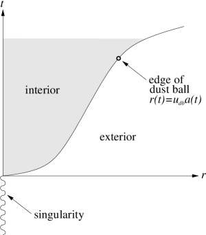
Figure 6: Evolution of the dust-ball and exterior regions in time, in Painlevé-Gullstrand coordinates.

In figure 6 we show the dust-ball and exterior regions of our model universe in PG coordinates. The equation of the surface is given by eq. (30), with $a(t)$ given in eq. (3). Note that prior to $t=0$, there is a singularity at $r=0$, as is evident from eq. (35).

The exterior metric may also be expressed in FRW-like coordinates with the use of the transformation (28); this results in

$$ds^{2}=dt^{2}-{\cal D}^{2}-a^{2}(t)u^{2}d\Omega^{\,2}\;,$$ (38)

where

$${\cal D}= \left(\frac{{\cal C}}{R_{d}\sinh(3t/2R_{d})}\right)^{\!\!1/3}\!\!\left\{u\left[\sqrt{\cosh^{2}(3t/2R_{d})+(u_{\scriptscriptstyle db}^{3}/u^{3}-1)}-\cosh(3t/2R_{d})\right]\,dt\right.$$ (39)

$$\left.\frac{}{}-R_{d}\sinh(3t/2R_{d})du\right\}\;.$$

Clearly, this joins smoothly to the dust-ball FRW metric at the surface $u=u_{\scriptscriptstyle db}$, as is evident from eqs. (1) and (3).

As a bonus, we point out that the above results apply also to the problem of the gravitational collapse of a uniform dust ball in a de Sitter background space; it is only necessary to reverse the sign of the PG time coordinate, or equivalently the sign of the cross term in the PG form of the metric [29].

In the next section, we will study the Kottler geometry in more detail, showing that it has peculiar and interesting properties when $2m_{u}\gg R_{d}$, which is the relevant case for our model.

5 Geometric nature of the exterior

In this section, we will use the Kottler metric as expressed in eq. (35) to investigate the geometrical nature of the exterior universe. Specifically, we will show that both the Schwarzschild and PG “time” coordinates, while algebraically convenient, are not acceptable time markers in the exterior space. Also, we will see that there is a rather interesting naked singularity at the origin for $t<0$.

Consider an observer at rest in the PG coordinates, with $dr=d\theta=d\phi=0$, so that the line element is

$$ds^{2}=\left(1-\frac{2m_{u}}{r}-\frac{r^{2}}{R_{d}^{\,2}}\right)\,dt^{2}\;.$$ (40)

If the $g_{00}$ component of the metric (in brackets) is positive, then the proper time interval $ds$ and the coordinate interval $dt$ are both real, so $t$ is an acceptable time marker. If $g_{00}$ is negative, then $t$ is not an acceptable time marker. The Kottler $g_{00}$ is plotted in figure 7 for two cases.

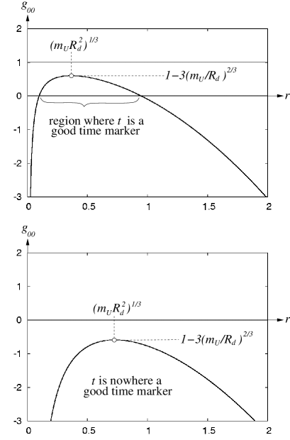
Figure 7: Metric component $g_{00}$ and the Painlevé “time” coordinate.

In the case $2m_{u}<(2/\sqrt{27})R_{d}$, it increases from minus infinity at $r=0$, lies between zero and one over some range of $r$, and then decreases to become negative again for large $r$ (figure 7, top). In the range where $g_{00}$ is positive, the coordinate $t$ is a useful time marker and we can interpret the metric as describing a Schwarzschild black hole in a de Sitter background. Indeed, if the geometric mass is much less than the de Sitter radius, that is $2m_{u}\ll(2/\sqrt{27})R_{d}$, then the coefficient in eq. (40) is zero near $2m_{u}$ and $R_{d}$, so the black-hole radius is near $2m_{u}$.

However, in the case of our model, $2m_{u}\gg(2/\sqrt{27})R_{d}$ and we see that $g_{00}$ is always negative, so that $t$ is not a useful time marker anywhere in space (figure 7, bottom). This situation is, of course, analogous to that of the standard Schwarzschild black-hole interior, which is better described using Kruskal-Szekeres coordinates than Schwarzschild coordinates. Accordingly, we now transform to new radial and time coordinates in which the metric is proportional, or conformal, to that of two-dimensional flat space with Lorentz coordinates. (In the rest of this section, we will deal only with the $t,r$ subspace, with angular coordinates suppressed.) We will refer to these as conformal coordinates for brevity. Since the light cones are the same as in two-dimensional special relativity, the causal structure of the space-time is quite transparent.

The metric (with angular parts suppressed) is

$$ds^{2}=(1-v^{2})\,dt^{2}+2v\,dr\,dt-dr^{2}\;,$$ (41)

so that radial null lines, or light rays, are described by

$$dt=\frac{dr}{(v\pm 1)}\;\;\;\;\;\;\mbox{(+ and -- null lines)}\;.$$ (42)

These null lines and some light cones are illustrated in figure 8.

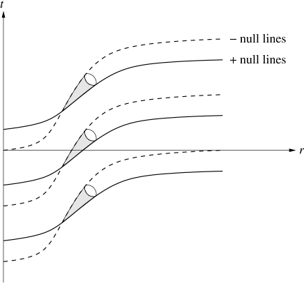
Figure 8: Null lines and schematic light cones in the Painlevé coordinates for a pure Kottler geometry.

Based on eq. (42), we introduce null coordinates defined by

$$\mu=t-\int_{0}^{r}\!\!\frac{dr^{\prime}}{v+1}\;\;\;,\;\;\;\lambda=\int_{0}^{r}\!\!\frac{dr^{\prime}}{v-1}-t\;\;\;,$$

$$d\mu=dt-\frac{dr}{v+1}\;\;\;,\;\;\;d\lambda=\frac{dr}{v-1}-dt\;.$$ (43)

Note that $d\mu=0$ and $d\lambda=0$ correspond to the $+$ and $-$ null lines, so that lines of constant $\mu$ or $\lambda$ represent light rays. From eqs. (43) we calculate the metric in the new coordinates to be

$$ds^{2}=(v^{2}-1)\,d\mu\,d\lambda\;,$$ (44)

in which $v$ is to be considered an implicit function of $\mu$ and $\lambda$ from eqs. (34) and (43).

To see the geometrical relation of the null coordinates to the PG coordinates, we consider some special lines, with the results shown in figure 9.

Figure 9: Some corresponding trajectories and points in PG and null conformal coordinates.

The figure shows only the exterior Kottler geometry, with no dust ball. Note that the combination

$$\mu+\lambda=2\int_{0}^{r}\frac{dr^{\prime}}{v^{2}-1}$$ (45)

is independent of $t$. In particular, the singular line $r=0$ corresponds to $\mu+\lambda=0$, while the line $r=\infty$ corresponds to

$$\mu+\lambda=2\int_{0}^{\infty}\!\!\!\frac{dr^{\prime}}{v^{2}-1}=2\int_{0}^{\infty}\!\!\!\frac{dr^{\prime}}{(2m_{u}/r^{\prime})+r^{\prime\,2}/R_{d}^{\,2}-1}\;\;\;\;\;\;(r=\infty)\;.$$ (46)

For $R_{d}\ll 2m_{u}$, the function $v^{2}$ is always much larger than one, so that the integral may be approximated by dropping the one in the denominator, with the result that

$$\mu+\lambda\approx 2R_{d}(R_{d}/2m_{u})^{1/3}\frac{2\pi}{3\sqrt{3}}\;\;\;\;\;\;(r=\infty)\;.$$ (47)

From the inequality (14), eq. (47) implies that

$$\mu+\lambda\approx\left[\frac{2\pi}{\sqrt{3}}\frac{(1-f)}{3.2}\right]\,R_{d}\leqslant\left[\frac{2\pi}{3.2\sqrt{3}}\right]\,R_{d}=1.1\,R_{d}\;.$$ (48)

That is, $\mu+\lambda$ is at most of order $R_{d}$. The entire physical space lies between the diagonal lines shown in figure 9. The + light ray emitted from the origin corresponds to $\mu=0$ and positive $\lambda$, while the – light ray emitted from the origin corresponds to $\lambda=0$ and positive $\mu$, as shown in the figure. Finally, the trajectory of a zero-energy dust particle emitted from the origin and obeying eq. (36) corresponds to the parametric curve

$$\mu=\int_{0}^{r}\frac{dr^{\prime}}{v}-\int_{0}^{r}\frac{dr^{\prime}}{v+1}=\int_{0}^{r}\frac{dr^{\prime}}{v^{2}+v}\;\;\;,\;\;\;\lambda=\int_{0}^{r}\frac{dr^{\prime}}{v-1}-\int_{0}^{r}\frac{dr^{\prime}}{v}=\int_{0}^{r}\frac{dr^{\prime}}{v^{2}-v}\;,$$ (49)

which is sketched in the figure. Of course, this also describes the dust-ball surface.

As our last change of coordinates, we rotate the $\mu,\lambda$ null coordinates by $45^{\circ}$ to obtain Lorentz-like coordinates $\tau,\rho$ defined by

$$\tau=(\lambda+\mu)/2=\int_{0}^{r}\!\!\frac{dr^{\prime}}{2m_{u}/r^{\prime}+r^{\prime\,2}/R_{d}^{\,2}-1}\;,$$

$$\rho=(\lambda-\mu)/2=\int_{0}^{r}\!\!\frac{\sqrt{2m_{u}/r^{\prime}+r^{\prime\,2}/R_{d}^{\,2}}\,dr^{\prime}}{2m_{u}/r^{\prime}+r^{\prime\,2}/R_{d}^{\,2}-1}-t\;.$$ (50)

In these coordinates, the metric is

$$ds^{2}=(v^{2}-1)(d\tau^{2}-d\rho^{2})\;.$$ (51)

The exterior space in these coordinates is shown in Fig 10 with some special lines indicated, and with the dust-ball region excised.

Figure 10: The exterior region in Lorentz-like coordinates. Only the region between the singularity and infinite future is physical, and similarly only the region from the dust-ball surface to infinite radial distance.

According to figure 10, we can view our model universe as a dust ball ejected from a singular hypersurface, which comprises all of 3-space at the initial time $\tau=0$. This singularity is analogous to the singularity of Schwarzschild geometry, which in Kruskal-Szekeres coordinates forms a future spacelike barrier to light and particles inside the black-hole surface. Note that the surface of the dust ball can be crossed by light and particles moving both inward and outward; that is, the interior of the dust ball can communicate with the exterior, and vice versa.

6 The early universe

The focus of this paper is on the present cosmic era and a universe dominated by dark energy and cold matter. We have not worked out the dynamics of the early universe in detail, but in this section we will briefly sketch an overal cosmic history that includes radiation-dominated and inflationary eras. Before the time of matter-radiation equality, at about $t_{\scriptscriptstyle E}\approx 10^{5}$ yr, the universe was dominated by radiation and relativistic or hot matter, with an approximate equation of state $p=\rho/3$. The scale function for hot matter is well known to take the form

$$a(t)\propto\sinh^{1/2}(t/2R_{d})\;\;\;\;\;\;\mbox{(radiation era)}\;.$$ (52)

This may be compared to the scale function during the matter-dominated era, eq. (3). Both are singular at $t=0$. During the radiation-dominated era, $t\ll R_{d}$ and the scale factor is well approximated by a constant times $a\propto t^{1/2}$. During the matter-dominated era, the scale function (3) is well approximated by a constant times $t^{2/3}$.

We can write the scale function for the early universe in a convenient and well known approximate form, if we assume that the energy density is entirely dominated by radiation (with $p=\rho/3$) before matter-radiation equality, and matter (with $p=0$) after this time. By matching the scale function and its derivatives at the time of equality, $t_{\scriptscriptstyle E}$, we obtain the expressions

$$a(t) \approx ({\cal C}^{1/3}\,2^{2/3}\,t_{\scriptscriptstyle E}^{1/6})\,t^{1/2}\;\;\;\;\;\;t_{\scriptscriptstyle I}<t<t_{\scriptscriptstyle E}\;\;\;\;\;\;\mbox{(fireball)}$$

$$a(t) \approx {\cal C}^{1/3}(3/2)^{2/3}(t+t_{\scriptscriptstyle E}/3)^{2/3}\;\;\;\;\;\;t>t_{\scriptscriptstyle E}\;\;\;\;\;\;\mbox{(early dust ball)}\;,$$ (53)

where ${\cal C}$ is the same constant of integration used in section 2, and $t_{\scriptscriptstyle I}$ is the time at which the inflationary era ends and the radiation-dominated one begins. We refer to the universe before $t_{\scriptscriptstyle E}$ as a fireball, to distinguish it from the dust ball that follows.

The mathematical problem is then to match the early fireball geometry to the exterior Kottler geometry, just as we matched the dust ball to the exterior in section 4. However this cannot be done in quite the same way, since there is pressure in the fireball, and thus a pressure gradient at the surface. The pressure gradient will eject material from the fireball surface, which will cool by expansion and radiation to form a cooler shell surrounding the ball. Hence the surface region will have a lower temperature and pressure. Indeed, for consistency with the time-independent exterior geometry obtained for the present era in section 4, the outer layers of the fireball must be at a reasonably low temperature and behave at least approximately like dust.

Clearly there is a wealth of further problems to be explored concerning the radiation-dominated era, including the density and pressure and temperature profiles of the fireball, as well as the effect of the finite size of the fireball on the CMB discussed in section 3. Such problems will probably require further and deeper use of the Einstein equations with the Einstein tensor given below in eqs. (59).

To summarize this part of the model: it seems plausible that the radiation-dominated era does not significantly alter the qualitative cosmic picture we have obtained for the present era; only the inner region of the fireball needs to be changed before the epoch of matter-radiation equality, as shown in the upper part of figure 11.

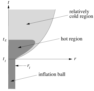
Figure 11: Schematic sketch of the early universe, including a hot radiation-dominated region and an inflationary region.

We next consider an inflationary era preceding the radiation-dominated one, as is currently popular. Inflation eliminates the singularity at $t=0$ and replaces it with a region of de Sitter-like geometry. The inflationary era is usually modeled in terms of one or more scalar fields, but is often described approximately with the use of a cosmological constant. Our model for this era is a ball of (static) de Sitter space, which we call an inflation ball, as shown in the lower part of figure 11.

We first calculate the Schwarzschild radius of the fireball at the end of inflation and beginning of the radiation-dominated era. The density of the matter and radiation in the fireball at this time is the difference between the vacuum-energy density $\rho_{\scriptscriptstyle I}$ during inflation and that in the present era ($\rho_{\,\scriptscriptstyle 0}$). We refer to all such matter as ponderable matter and write its density as follows:

$${\rho}_{\scriptscriptstyle{\rm pond}}=\rho_{\scriptscriptstyle I}-\rho_{\,\scriptscriptstyle 0}=\frac{3}{8\pi GR_{\scriptstyle I}^{\,2}}-\frac{3}{8\pi GR_{d}^{\,2}}\;,$$ (54)

where $R_{\scriptstyle I}$ is the de Sitter radius during inflation, a number typically taken to be of order $10^{-26}$ m. The Schwarzschild radius is obtained from this density as

$$2m_{u}=2GM_{u}=2G\left(\frac{4\pi r_{\scriptscriptstyle I}^{3}}{3}\right){\rho}_{\scriptscriptstyle{\rm pond}}=r_{\scriptscriptstyle I}^{3}\left(\frac{1}{R_{\scriptstyle I}^{\,2}}-\frac{1}{R_{d}^{\,2}}\right)\;,$$ (55)

where $r_{\scriptscriptstyle I}$ denotes the initial radius of the fireball.

For the inflationary era, the scale function is an exponential, which we write as

$$a(t)=({\cal C}^{1/3}\,2^{2/3}\,t_{\scriptscriptstyle E}^{1/6}\,t_{\scriptscriptstyle I}^{1/2})\,e^{(t-t_{\scriptscriptstyle I})/R_{\scriptstyle I}}\;,\;\;\;\;\;\;t<t_{\scriptscriptstyle I}\;.$$ (56)

The coefficient here is chosen in such a way as to match the scale function and its derivative at the beginning of the radiation-dominated era (time $t_{\scriptscriptstyle I}$). From the transformation (28), we find that the corresponding PG metric function is

$$v=(\dot{a}/a)r=r/R_{\scriptstyle I}\;.$$ (57)

This represents static de Sitter space. We must now equate this function $v$ to the exterior function $v$ in eq. (34) at the surface of the inflation ball. Since both functions depend only on radius, the equality must hold along a line of constant radius $r_{\scriptscriptstyle I}$ given by

$$v=\sqrt{\frac{2m_{u}}{r_{\scriptscriptstyle I}}+\frac{r_{\scriptscriptstyle I}^{2}}{R_{d}^{\,2}}}=\frac{r_{\scriptscriptstyle I}}{R_{\scriptstyle I}}\;,\;\;\;\;\;\;2m_{u}=r_{\scriptscriptstyle I}^{3}\left(\frac{1}{R_{\scriptstyle I}^{\,2}}-\frac{1}{R_{d}^{\,2}}\right)\;.$$ (58)

Remarkably, this is the same relation that we found in eq. (55), which resulted from energy conservation. The inflation ball thus has a constant radius, as shown in figure 11.

The above matching of the inflation-ball geometry to the exterior is quite unlike the matching that we used for the present era, in which the interior and exterior metrics matched along a test-particle (or dust-particle) geodesic. The reason for the difference is that the inflation ball has surface tension. To see this, we note that the function $v$ is continuous at the inflation-ball surface according to eq. (58), but that its derivative is not. The discontinuity in the derivative produces a singular stress-energy tensor at the surface, which can be calculated from the Einstein equations $T_{\mu}^{\nu}=-G_{\mu}^{\nu}/(8\pi G)$. It is only slightly tedious to calculate the Einstein tensor for the PG form of the metric, with the results [29]

$$G_{0}^{0}=-\frac{2vv^{\prime}}{r}-\frac{v^{2}}{r^{2}}\;,\;\;\;\;\;\;G_{0}^{1}=\frac{2v\dot{v}}{r}\;,$$

$$G_{1}^{1}=-\frac{2vv^{\prime}}{r}-\frac{v^{2}}{r^{2}}-\frac{2\dot{v}}{r}\;,\;\;\;\;\;\;G_{2}^{2}=G_{3}^{3}=-\frac{2vv^{\prime}}{r}-\frac{\dot{v}}{r}-\dot{v}^{\prime}-v^{\prime\prime}v-v^{\prime 2}\;.$$ (59)

Here primes denote radial derivatives while the overdot represents a derivative with respect to time. Using these expressions together with eqs. (57) and (58), we find that the stress-energy tensor on the surface has only two nonzero components:

$$T_{2}^{2}=T_{3}^{3}=-\frac{3m_{u}}{8\pi G}\,\delta(r-r_{\scriptscriptstyle I})\;.$$ (60)

This represents precisely the tangential stress at the surface of a fluid; that is, surface tension. It is essentially the same as the force holding a balloon in equilibrium [29].

To summarize this part of the model, we may view the inflationary phase of our model in PG coordinates as a small ball of de Sitter space, which gives rise to the fireball and later the dust ball that make up our universe, as depicted in figure 11. If one accepts the inflationary paradigm, then the initial singularity discussed in sections 4 and 5 may be thought of as a rough phenomenological description of a region of de Sitter space.

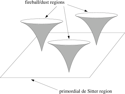
Figure 12: A somewhat fanciful view of cosmogenesis, based on the exterior space in conformal coordinates shown in figure 10 but modified to include a de Sitter region.

We note finally that the physical picture of cosmogenesis that was discussed briefly in section 5 based on conformal coordinates should now be modified so that the 3-space-filling singularity is replaced by a spacelike region of primordial de Sitter space, as illustrated schematically in figure 12 (compare figs. 9 and 10). Our region of the universe, and cosmic time, begin as an exploding ball of fire which cools to a dust ball, as shown in the figure. There is no reason why such an initial state should not give rise to more than one such exploding fireball, or why the fireballs produced in this way should not be able to communicate with each other, or even to merge — a feature that critically distinguishes this finite-universe model from superficially similar proposals by many other authors involving multiverses (see [30] and references therein).

7 Summary and conclusions

We have presented what is effectively a truncated version of the standard concordance cosmology, one that might be termed a “truncordance model” for short. This model goes over to the conventional one in the limit of a large dust ball in which we are not too close to the edge, as should be expected. It presents many intriguing features, which we have explored using various coordinate systems. We have only sketched how the model can be extended to encompass earlier inflationary and radiation-dominated eras. Perhaps most satisfyingly, our model offers the possibility of experimental testability, at least in principle, a feature which distinguishes it from other suggestions of recent years.

References

- [1] R.J. Adler and J.M. Overduin, Gen. Rel. Grav. 37 (2005) 1491
- [2] L.-Y. Chiang et al., Ap. J. 590 (2003) L65
- [3] D.L. Larson and B.D. Wandelt, Phys. Rev. D., submitted; astro-ph/0505046
- [4] R. Tojeiro et al., Mon. Not. R. Astron. Soc. 365 (2006) 265; astro-ph/0507096
- [5] A. Bernui et al., astro-ph/0511666
- [6] H.K. Eriksen et al., Astrophys. J. 605 (2004) 14; astro-ph/0307507
- [7] H.K. Eriksen et al., Astrophys. J. 612 (2004) 64; astro-ph/0401276
- [8] F.K. Hansen et al., Astrophys. J. 607 (2004) L67; astro-ph/0402396
- [9] F.K. Hansen, A.J. Banday and K.M. Górski, Mon. Not. R. Astron. Soc. 354 (2004) 641; astro-ph/0404206
- [10] F.K. Hansen et al., Mon. Not. R. Astron. Soc. 354 (2004) 905; astro-ph/0406232
- [11] C.J. Copi et al., astro-ph/0508047
- [12] P.E. Freeman et al., Astrophys. J. 638 (2005) 1; astro-ph/0510406
- [13] X. Liu and S.N. Zhang, Astrophys. J. 636 (2006) L1; astro-ph/0511550
- [14] P. Vielva et al., Astrophys. J. 609 (2004) 22; astro-ph/0310273
- [15] M. Cruz et al., Mon. Not. R. Astron. Soc. 356 (2005) 29; astro-ph/0405341
- [16] J.D. McEwen et al., Mon. Not. R. Astron. Soc. 359 (2005) 1583; astro-ph/0406604
- [17] K.T. Inoue and J. Silk, astro-ph/0602478
- [18] L. Cayón , J. Jin and A. Treaster, Mon. Not. R. Astron. Soc. 362 (2005) 826; astro-ph/0507246
- [19] M. Cruz et al., astro-ph/0601427
- [20] K. Tomita, Phys. Rev. D72 (2005) 103506; erratum Phys. Rev. D73 (2006) 029901; astro-ph/0509518
- [21] J.D. McEwen et al., astro-ph/0510349
- [22] G. Efstathiou, Mon. Not. R. Astron. Soc. 343 (2003) L95 [astro-ph/0303127]
- [23] J.-P. Uzan, U. Kirchner and G.F.R. Ellis, Mon. Not. R. Astron. Soc. 344 (2003) L65 [astro-ph/0302597]
- [24] J.-P. Luminet, astro-ph/0501189
- [25] P. Painlevé, Comptes Rendus Acad. Sci. (Paris) 173 (1921) 677
- [26] A. Gullstrand, Arkiv. Mat. Astron. Fys. 16 (1922) 1
- [27] F. Kottler, Ann. Phys. (Berlin) 56 (1918) 401
- [28] H. Weyl, Phys. Zeits. 20 (1919) 31
- [29] R.J. Adler et al., Am. J. Phys. 73 (2005) 1148
- [30] W.R. Stoeger, astro-ph/0602356