IGPG–06/2–2
AEI–2006–009
gr–qc/0602100

Quantum Riemannian Geometry
and Black Holes
Martin Bojowald
Institute for Gravitational Physics and Geometry, The Pennsylvania State University, 104 Davey Lab, University Park, PA 16802, USA;

Max-Planck-Institut für Gravitationsphysik, Albert-Einstein-Institut,

Am Mühlenberg 1, D-14476 Potsdam, Germany

Abstract

Black Holes have always played a central role in investigations of quantum gravity. This includes both conceptual issues such as the role of classical singularities and information loss, and technical ones to probe the consistency of candidate theories. Lacking a full theory of quantum gravity, such studies had long been restricted to black hole models which include some aspects of quantization. However, it is then not always clear whether the results are consequences of quantum gravity per se or of the particular steps one had undertaken to bring the system into a treatable form. Over a little more than the last decade loop quantum gravity has emerged as a widely studied candidate for quantum gravity, where it is now possible to introduce black hole models within a quantum theory of gravity. This makes it possible to use only quantum effects which are known to arise also in the full theory, but still work in a rather simple and physically interesting context of black holes. Recent developments have now led to the first physical results about non-rotating quantum black holes obtained in this way. Restricting to the interior inside the Schwarzschild horizon, the resulting quantum model is free of the classical singularity, which is a consequence of discrete quantum geometry taking over for the continuous classical space-time picture. This fact results in a change of paradigm concerning the information loss problem. The horizon itself can also be studied in the quantum theory by imposing horizon conditions at the level of states. Thereby one can illustrate the nature of horizon degrees of freedom and horizon fluctuations. All these developments allow us to study the quantum dynamics explicitly and in detail which provides a rich ground to test the consistency of the full theory.

Contents

1. 1 Introduction
2. 2 Spherical Symmetry
   1. 2.1 Metric and triad
   2. 2.2 Basic variables
   3. 2.3 Dynamics
3. 3 Quantization: Overview
   1. 3.1 Homogeneous techniques
   2. 3.2 Extrapolation
   3. 3.3 Inhomogeneous techniques
   4. 3.4 Full theory
4. 4 Homogeneous techniques
   1. 4.1 Quantum representation
   2. 4.2 Inverse triad components
   3. 4.3 Dynamics
   4. 4.4 Effective dynamics
5. 5 Extrapolation
6. 6 Inhomogeneous techniques
   1. 6.1 Hamiltonian constraint
   2. 6.2 Dynamics
   3. 6.3 Horizons
      1. 6.3.1 Definition
      2. 6.3.2 Spherical symmetry
      3. 6.3.3 Dynamics
7. 7 Full theory
   1. 7.1 Representation
   2. 7.2 Black hole entropy
8. 8 Conclusion
9. Acknowledgements

1 Introduction

Black holes in classical general relativity are, compared to other astrophysical objects, distinguished by the presence of singularities, where curvature and tidal forces diverge and where space-time stops, and horizons, which can separate off regions from causal contact from another region. Both properties have long been suspected to be changed in a quantum theory of gravity: Singularities denote points where the classical theory breaks down, and at least space-like ones which lie to the past or future of observers are supposed to be removed in a more complete quantum theory. Horizons, on the other hand, are still expected to play an important role also in quantum gravity. The horizon surface should at most be smeared out due to fluctuations in the causal structure on which the concept of horizons relies. For massive black holes (compared to the Planck mass) these horizon fluctuations should be negligible for most purposes such that the classical picture still applies. Instead of modifying the horizon on large scales, quantum gravity is expected to provide a microscopic picture which shows how to build a macroscopic horizon from Planck scale ingredients. If successful, this will then result in a statistical explanation of black hole entropy.

In more detail, the main issues concerning black holes in quantum gravity are as follows:

Singularities:

Are they indeed removed and, if yes, what replaces them? There are arguments that not all singularities are equal, with space-like ones to be removed and time-like ones to persist in order to rule out unwanted (such as negative mass) solutions [1]. Also the issue of naked singularities and cosmic censorship arises in this context.

Horizons:

First of all, one has to see what an adequate definition of a horizon in quantum gravity could be. The original concept of the event horizon relies on the classical causal structure of all of space-time as well as the presence of singularities in the future. The quasi-local concept of isolated or dynamical horizons [2] uses much weaker assumptions about the structure of space-time such that it is better suited to a quantum treatment at least for large, semiclassical black holes which have only weak curvature at the horizon. For microscopic or primordial black holes, space-time even around the horizon cannot be treated as a smooth classical geometry with a classical causal structure. Here it is not clear if a quantum concept of horizon can even be applied.

If there is an applicable notion of quantum horizon, the issue of black hole entropy can be analyzed. By identifying and counting quantum states uniquely characterizing a horizon of a given area one can compute black hole entropy and compare with the expected semiclassical Bekenstein–Hawking formula. Moreover, detailed pictures of the horizon structure and its fluctuations can be developed which shed more light on quantum gravity in general. If matter fields are present, the horizon should shrink from Hawking radiation which provides insights on how gravity interacts with matter at the quantum level.

Both:

Systems such as black holes with singularities as well as horizons have led to much confusion in attempts to guess the outcome of quantum gravity from early glimpses obtained from mainly semiclassical considerations. This is most commonly expressed in the infamous information loss paradox according to which information falling into the singularity implies a non-unitary quantum evolution and thus presumably fundamental limitations to knowledge [3]. These ideas obviously do not take into account what happens to singularities in quantum gravity and thus have to be revisited once a more complete treatment is available.

All these issues probe different aspects of the full theory of quantum gravity and require different techniques. A common feature, except for the entropy counting of isolated horizons, is that they are dynamical aspects such that the Hamiltonian constraint operator in a canonical quantization or an alternative evolution equation is essential. In particular, both black hole singularities as well as their horizons require inhomogeneous situations and an approximation by spatial homogeneity, which works well in cosmological cases, is not sufficient in general to grasp all the important physical aspects. This has the advantage of providing many non-trivial tests of quantum gravity which go beyond what is possible in homogeneous cosmological models.

It certainly also implies that the treatment is more complicated, and indeed progress on the problems listed here has been mixed. The strongest results exist for the counting of black hole entropy of static or isolated horizons which has been derived in different approaches [4, 5, 6, 7, 8]. This has been possible since the isolation (or even extremality in [4]) allows one to ignore the complicated quantum dynamics and still compute the correct number of physical states. Moreover, only the horizon itself is important such that its inhomogeneous neighborhood does not have much influence. This changes if one also wants to study, e.g., horizon fluctuations since they are dynamical and require the neighborhood in which the horizon fluctuates. Thus, both the quantum dynamics and inhomogeneous configurations have to be handled, and there are not many results within a full candidate of quantum gravity so far.

Similarly, the issue of singularities relies on dynamical aspects which for most of the time was too complicated to allow definitive conclusions as to whether or not singularities persist in quantum gravity. In the last few years, there has been progress on the homogeneous situation of cosmological singularities [9, 10, 11] which have been shown to be removed by quantum gravity [12]. Analogous techniques are now also available for some inhomogeneous situations such as the spherically symmetric model [13, 14] which is classically relevant for non-rotating black holes. This has led to an extension of the non-singularity statements from homogeneous models to the spherically symmetric one [15]. Moreover, with new results about quantum horizons a consistent picture of quantum physics of black holes is emerging.

This chapter is also intended as an introduction, by way of examples, to some of the techniques of quantum geometry with an emphasis on aspects which are typical for a loop quantization and essential for physical issues. The main theme will be the understanding of quantum dynamics in inhomogeneous situations and problems surrounding it.

2 Classical aspects of spherically symmetric systems

A spherically symmetric metric is most easily written in polar coordinates $(x,\vartheta,\varphi)$ and takes the form (with ${\mathrm{d}}\Omega^{2}={\mathrm{d}}\vartheta^{2}+\sin^{2}\vartheta{\mathrm{d}}\varphi^{2}$)

$${\mathrm{d}}s^{2}=-N(x,t)^{2}{\mathrm{d}}t^{2}+q_{xx}(x,t)({\mathrm{d}}x+N^{x}(x,t){\mathrm{d}}t)^{2}+q_{\varphi\varphi}(x,t){\mathrm{d}}\Omega^{2}$$ (1)

where fields only depend on time $t$ and the coordinate $x$ of the 1-dimensional radial manifold $B$. This expression makes use of the lapse function $N(x,t)$ and shift vector $N^{x}(x,t)$ which are prescribed by the slicing of space-time into spatial constant-$t$ slices: coordinate time translations are generated by the vector field

$$\frac{\partial}{\partial t}=Nn+N^{x}\frac{\partial}{\partial x}$$ (2)

with the unit vector field $n$ being normal to the slices. The spatial metric on those slices is then

$${\mathrm{d}}q^{2}=q_{xx}(x,t){\mathrm{d}}x^{2}+q_{\varphi\varphi}(x,t){\mathrm{d}}\Omega^{2}$$ (3)

and extrinsic curvature

$$K_{ab}={\textstyle\frac{1}{2}}{\cal L}_{n}q_{ab}\,,$$ (4)

which determines the conjugate $\pi^{ab}=-\frac{1}{2}\sqrt{\det q}(K^{ab}-q^{ab}K^{c}_{c})$ to the metric in a canonical formulation [16], takes a similar form $K=K_{xx}(x,t){\mathrm{d}}x^{2}+K_{\varphi\varphi}(x,t){\mathrm{d}}\Omega^{2}$.

A well-known example is obtained by the spherically symmetric vacuum solution to Einstein’s field equations, the Schwarzschild metric [17]

$${\mathrm{d}}s^{2}=-(1-2M/x){\mathrm{d}}t^{2}+\frac{1}{1-2M/x}{\mathrm{d}}x^{2}+x^{2}{\mathrm{d}}\Omega^{2}$$ (5)

with the mass parameter $M$. It has the following properties: If we first restrict our attention to larger $x>2M$, the metric is static since its coefficients do not depend on time and $N^{x}=0$. When $x$ becomes large compared to the mass, i.e. if we approach the asymptotic regime far away from the black hole, the metric becomes asymptotically flat. The black hole region is characterized by the horizon which appears at $x=2M$ as a coordinate singularity in the Schwarzschild metric and can be defined in a coordinate independent manner as the outer boundary of a region where trapped surfaces, i.e. envelops of light rays which cannot expand outwards to infinity, occur. If we enter the black hole region through the horizon we notice that now $t$ becomes a space-like coordinate since the $tt$ component changes sign. The role of coordinate time is then played by $x$ on which the metric coefficients depend. Thus, the interior is not static, but since the metric components now do not depend on the spatial coordinate $t$ it is homogeneous (of Kantowski–Sachs form).

2.1 Metric and triad

The metric components $q_{\varphi\varphi}=x^{2}$, $q_{xx}=(1-2M/x)^{-1}$ and $N^{2}=-g_{tt}=1-2M/x$ can be used to characterize the three different regimes of a massive black hole with mass $M\gg 1$: At asymptotic infinity we have $x\gg 2M\gg 1$ and thus

$$q_{\varphi\varphi}\gg 1\qquad q_{xx}\sim 1\,.$$

At the horizon we have $x\sim 2M$ and

$$q_{\varphi\varphi}\gg 1\qquad q_{xx}\gg 1$$

while at the singularity we have $0\sim x\ll 2M$ and

$$q_{\varphi\varphi}\ll 1\qquad|q_{xx}|\ll 1\qquad N\gg 1\,.$$

In the latter case, $q_{xx}$ is relevant only if we approach the singularity on slices with $t$ constant which are time-like inside the horizon. The lapse function, on the other hand, is the relevant metric component if we approach the singularity on slices which are space-like inside.

These regimes of metric components can be used for a first glimpse on how a quantization may deal with the singularity or horizon. From cosmological models it is known that expressions for, e.g., curvature components can be modified when they become large, cutting off classical divergences (in isotropic cosmology they are all inverse powers of the scale factor [18], or spin connection components in anisotropic models [11]). Similarly here, some spin connection components contain information about intrinsic curvature. Their form can be obtained from the general expression (see, e.g., [19])

$$\Gamma_{a}^{i}=-\epsilon^{ijk}e^{b}_{j}(\partial_{[a}e_{b]}^{k}+{\textstyle\frac{1}{2}}e_{k}^{c}e_{a}^{l}\partial_{[c}e_{b]}^{l})$$ (6)

where $e_{a}^{i}$ are components of the co-triad (i.e. $e_{a}^{i}e_{b}^{i}=q_{ab}$) and $e^{b}_{j}$ of its inverse. In spherical symmetry, co-triads take a special form just as the metric (3) does. Since it does not matter how a triad is rotated, it need not be exactly invariant under the rotation group acting on space, but it is enough for it to be invariant up to a gauge rotation. This is realized for co-triads of the form

$$e_{a}^{i}\tau_{i}{\mathrm{d}}x^{a} = e_{x}(x)\tau_{3}{\mathrm{d}}x+(e_{1}(x)\tau_{1}+e_{2}(x)\tau_{2}){\mathrm{d}}\vartheta+(e_{1}(x)\tau_{2}-e_{2}(x)\tau_{1})\sin\vartheta{\mathrm{d}}\varphi$$ (7)

$$=: e_{x}(x)\tau_{3}{\mathrm{d}}x+e_{\varphi}(x)\bar{\Lambda}(x){\mathrm{d}}\vartheta+e_{\varphi}(x)\Lambda(x)\sin\vartheta{\mathrm{d}}\varphi$$

where we use SU(2) generators $\tau_{j}=-\frac{i}{2}\sigma_{j}$ with Pauli matrices $\sigma_{j}$, and $\Lambda=:\cos\eta\tau_{2}+\sin\eta\tau_{1}$ and $\bar{\Lambda}:=\exp(-\frac{\pi}{2}\tau_{3})\Lambda\exp(\frac{\pi}{2}\tau_{3})$ are defined to have unit norm in su(2), i.e. $\cos\eta=e_{1}/e_{\varphi}$ and $\sin\eta=-e_{2}/e_{\varphi}$ with $e_{\varphi}^{2}=e_{1}^{2}+e_{2}^{2}$. Infinitesimal rotations of space now act by Lie derivatives on $e$ with respect to superpositions of vector fields $X=\sin\varphi\partial_{\vartheta}+\cot\vartheta\cos\varphi\partial_{\varphi}$, $Y=-\cos\varphi\partial_{\vartheta}+\cot\vartheta\sin\varphi\partial_{\varphi}$, and $Z=\partial_{\varphi}$, while gauge rotations of the triad act by conjugation in su(2). We thus obtain explicitly

$${\cal L}_{X}e = (e_{1}\tau_{1}+e_{2}\tau_{2})\cos\varphi{\mathrm{d}}\varphi-(-e_{2}\tau_{1}+e_{1}\tau_{2})\frac{\cos\varphi}{\sin\vartheta}{\mathrm{d}}\vartheta=\left[e,\frac{\cos\varphi}{\sin\vartheta}\tau_{3}\right]$$

$${\cal L}_{Y}e = (e_{1}\tau_{1}+e_{2}\tau_{2})\sin\varphi{\mathrm{d}}\varphi-(-e_{2}\tau_{1}+e_{1}\tau_{2})\frac{\sin\varphi}{\sin\vartheta}{\mathrm{d}}\vartheta=\left[e,\frac{\sin\varphi}{\sin\vartheta}\tau_{3}\right]$$

$${\cal L}_{Z}e = 0$$

showing that any rotation in space simply amounts to a gauge rotation of the triad. The corresponding metric is thus invariant under rotations, and indeed a co-triad (7) implies a metric of the form (3) with

$$q_{xx}=e_{x}^{2}\quad,\quad q_{\varphi\varphi}=e_{1}^{2}+e_{2}^{2}=e_{\varphi}^{2}\,.$$ (8)

A spherically symmetric spin connection takes the form

$$\Gamma_{a}^{i}\tau_{i}{\mathrm{d}}x^{a}=\Gamma_{x}\tau_{3}{\mathrm{d}}x+\Gamma_{\varphi}\bar{\Lambda}^{\Gamma}{\mathrm{d}}\vartheta+\Gamma_{\varphi}\Lambda^{\Gamma}\sin\vartheta{\mathrm{d}}\varphi+\tau_{3}\cos\vartheta{\mathrm{d}}\varphi$$ (9)

where the last term must be added since a connection transforms differently from a co-triad under gauge transformations. Indeed,

$${\cal L}_{X}(\tau_{3}\cos\vartheta{\mathrm{d}}\varphi) = -\tau_{3}\left(\frac{\sin\varphi}{\sin\vartheta}{\mathrm{d}}\varphi+\frac{\cos\vartheta\cos\varphi}{\sin^{2}\vartheta}{\mathrm{d}}\vartheta\right)={\mathrm{d}}\left(\frac{\cos\varphi}{\sin\vartheta}\tau_{3}\right)$$

$${\cal L}_{Y}(\tau_{3}\cos\vartheta{\mathrm{d}}\varphi) = -\tau_{3}\left(\frac{\cos\varphi}{\sin\vartheta}{\mathrm{d}}\varphi-\frac{\cos\vartheta\sin\varphi}{\sin^{2}\vartheta}{\mathrm{d}}\vartheta\right)={\mathrm{d}}\left(\frac{\sin\varphi}{\sin\vartheta}\tau_{3}\right)$$

and ${\cal L}_{Z}(\tau_{3}\cos\vartheta{\mathrm{d}}\varphi)=0$ such that we have the correct transformation of $\Gamma$ with the same gauge rotation as above.

The explicit formula (6) applied to a spherically symmetric co-triad shows that

$$\Gamma_{x}=-\eta^{\prime}\quad,\quad\Gamma_{\varphi}=-e_{\varphi}^{\prime}/e_{x}\quad,\quad\Lambda^{\Gamma}=\bar{\Lambda}\,,$$ (10)

with $\bar{\Lambda}$ as defined for the co-triad, such that the $\varphi$-component $\Gamma_{\varphi}$ is gauge invariant while $\Gamma_{x}$ is pure gauge. Modifications to classical behavior similar to those in cosmological models can now be expected, e.g., from the spin connection component $\Gamma_{\varphi}=-\sqrt{q_{\varphi\varphi}}^{\prime}/\sqrt{q_{xx}}$ when metric components become small. Classically, this expression diverges at small $q_{xx}$, which can be changed in a quantum theory for the corresponding operator. Since, as we will see later, $\Gamma_{\varphi}$ appears in the equations of motion, a modification here would change the behavior of solutions. Horizons of massive black holes would remain unmodified since there both metric components are large. The singularity, however, looks less clear: only for time-like slices does $q_{xx}$ become small, indicating a modification and the possibility of removal of the singularity. But if we approach the singularity on space-like slices with $x$ constant, in the interior $N^{2}$ (playing then the role of $q_{xx}$) remains large which does not suggest modifications. Indeed, the slices then are homogeneous and $\Gamma_{\varphi}$ vanishes identically which means that we will need another measure for the removal of singularities in this case.

At asymptotic infinity, however, we would encounter severe problems since $q_{xx}$ is close to one at which point modifications can already be noticeable, spoiling the classical limit of the theory. This is a sign of using the wrong variables since the modification is a consequence of quantum effects, and the success of a quantization can depend significantly on the choice of fundamental variables. Indeed, there are variables better suited to a demarkation of the different regimes than the metric. This is in particular the case for the densitized triad defined by $E^{a}_{i}=e^{a}_{i}|\det(e_{b}^{j})|$ where $e^{a}_{i}$ is the inverse of the co-triad $e$ compatible with the metric. A spherically symmetric densitized triad is of the general form

$$E=E^{x}(x)\tau_{3}\sin\vartheta\frac{\partial}{\partial x}+(E^{1}(x)\tau_{1}+E^{2}(x)\tau_{2})\sin\vartheta\frac{\partial}{\partial\vartheta}+(E^{1}(x)\tau_{2}-E^{2}(x)\tau_{1})\frac{\partial}{\partial\varphi}$$ (11)

written down as an su(2) valued densitized vector field. The gauge invariant components are $E^{x}$ and $(E^{\varphi})^{2}=(E^{1})^{2}+(E^{2})^{2}$ whose relation with the metric components is

$$|E^{x}|=q_{\varphi\varphi}\qquad E^{\varphi}=\sqrt{q_{xx}q_{\varphi\varphi}}$$ (12)

(note that $E^{x}$ can be positive or negative depending on the orientation $\mathop{\mathrm{sgn}}\det E=\mathop{\mathrm{sgn}}E^{x}(E^{\varphi})^{2}$ of the triad). The angular components have the same internal directions $\Lambda$ and $\bar{\Lambda}$ as the co-triad.

For the Schwarzschild solution with $|E^{x}|=x^{2}$ and $E^{\varphi}=x/\sqrt{1-2M/x}$ we now have the following behavior: At asymptotic infinity

$$|E^{x}|\gg 1\qquad E^{\varphi}\gg 1\,,$$

at the horizon

$$|E^{x}|\gg 1\qquad E^{\varphi}\gg 1$$

and at the singularity

$$|E^{x}|\ll 1\qquad E^{\varphi}\ll 1\,.$$

Thus, irrespective of the approach to the singularity, the behavior is just as needed for unmodified classical behavior far away from the black hole all the way up to the horizon, while inverse triad components, such as the spin connection component

$$\Gamma_{\varphi}=-(E^{x})^{\prime}/2E^{\varphi}$$ (13)

will be modified at the singularity with small $E^{\varphi}$.

2.2 Basic variables

For detecting the classical singularity it seems much more reliable to use the densitized triad rather than the metric, which is also the case in homogeneous models with an explicit impact on the removal of singularities [10]. Indeed, the densitized triad as a basic variable is important in other ways, too: it arises naturally when one attempts to quantize gravity in a background independent manner. These two issues, the fate of classical singularities and background independence, are superficially quite different but turn out to be deeply related.

Most recent progress in a background independent quantization of general relativity has come after a reformulation in terms of Ashtekar variables [20, 21] where the densitized triad $E^{a}_{i}$ plays the role of a momentum canonically conjugate to the Ashtekar connection $A_{a}^{i}=\Gamma_{a}^{i}-\gamma K_{a}^{i}$ with the spin connection $\Gamma_{a}^{i}$ as a function of $E^{a}_{i}$ via (6), extrinsic curvature $K_{a}^{i}=e^{b}_{i}K_{ab}$ and the Barbero–Immirzi parameter $\gamma>0$ [22]. The extrinsic curvature components here make $A_{a}^{i}$ canonically conjugate to $E^{a}_{i}$, while the spin connection provides $A_{a}^{i}$ with the transformation properties of a connection. This reformulation thus casts general relativity as a gauge theory and does not only bring it formally closer to other interactions but also leads to a direct way for a background independent quantization.

Usually, a field theory would be quantized by smearing the fields with test functions over 3-dimensional regions so as to make their classical Poisson *-algebra well defined. For instance, a scalar $\phi$ with Lagrangian $\sqrt{\det q}(\frac{1}{2}\dot{\phi}^{2}+\frac{1}{2}q^{ab}\partial_{a}\phi\partial_{b}\phi+V(\phi))$ on a background metric $q_{ab}$ (assuming lapse function $N=1$ and shift vector $N^{a}=0$) has momentum $p_{\phi}=\sqrt{\det q}\dot{\phi}$ which transforms as a density (which is often ignored when the background metric is fixed as, e.g., Minkowski space). This has the singular Poisson relations $\{\phi(x),p_{\phi}(y)\}=\delta(x,y)$. However, if we smear the fields with test functions $f$ and $g$ on space to obtain $\phi[f]:=\int\sqrt{\det q}f(x)\phi(x){\mathrm{d}}^{3}x$ and $p_{\phi}[g]:=\int g(x)p_{\phi}(x){\mathrm{d}}^{3}x$ we obtain the well-defined Poisson algebra $\{\phi[f],p_{\phi}[g]\}=\int\sqrt{\det q}f(x)g(x){\mathrm{d}}^{3}x$. This does not contain $\delta$-functions, but does depend on the background metric $q$ which is not available for a background independent formulation of gravity. The very first step of a background independent quantization of general relativity, therefore, has to face the problem that the physical fields, with the metric or densitized triad among them, need to be smeared for a well-defined algebra to be represented on a Hilbert space, but that a background metric must not be introduced.

For a scalar, there is a simple way out: as is easily verified, we still obtain a well-defined algebra if we only smear $p_{\phi}$ for which we do not need a background metric since it is already a density. Similarly, in the case of gravity we can evade the problem in Ashtekar’s formulation since with connections and densitized vector fields as basic variables there is a natural, background independent smearing leading to a well-defined algebra: Instead of 3-dimensional smearings for all basic fields we use a 1-dimensional smearing of the connection and a 2-dimensional one for the densitized triad, giving rise to holonomies

$$h_{e}(A)={\cal P}\exp\int_{e}\tau_{i}A_{a}^{i}\dot{e}^{a}{\rm d}t$$ (14)

along edges $e$ in space, and fluxes

$$F_{S}(E)=\int_{S}\tau^{i}E^{a}_{i}n_{a}{\rm d}^{2}y$$ (15)

through surfaces $S$. (We use the tangent vector $\dot{e}^{a}$ to the curve $e$ and the co-normal $n_{a}$ to the surface $S$, both of which are defined without reference to a metric.)

It turns out that this smearing is sufficient for a well-defined classical Poisson algebra which even has a unique diffeomorphism invariant representation [23, 24, 25, 26, 27]. This representation defines the basic framework of loop quantum gravity [28, 29, 30, 31]. States are represented usually in the connection representation $\psi[A]$ on which holonomies act as multiplication operators and fluxes as derivative operators. This can all be done rigorously thanks to a rich structure on the infinite dimensional space of connections which is under much better control than the space of metrics. As a consequence, flux operators have discrete spectra implying a discrete structure of spatial geometry [32, 33, 34] which is also realized in symmetric models [35, 36]. Moreover, since flux spectra are discrete and contain zero, there are no densely defined inverse operators. Instead there are techniques [37] which allow one to quantize co-triad or other inverse components of the basic $E^{a}_{i}$ by operators which reduce to the inverse in a classical regime but modify the classical divergence at small values. This has already been described and used above for the spherically symmetric spin connection component. Here, it is important that those expressions are taken as functions of the densitized triad components and not metric components. These effects come from properties of flux operators as basic operators in a background independent formulation which relies on the densitized triad as basic variable and so far is not known in a metric formulation. Indeed, as observed before, the densitized triad is much better suited to separate the classical singularity from other regimes such that modifications are only expected there.

2.3 Dynamics

Up until now we have discussed kinematical properties of the spherically symmetric system. The dynamical behavior of triad and connection (or extrinsic curvature) components is dictated by the Hamiltonian constraint

$$H[N]=(2G)^{-1}\int_{B}{\mathrm{d}}xN(x)|E^{x}|^{-1/2}\left((K_{\varphi}^{2}E^{\varphi}+2K_{\varphi}K_{x}E^{x})+(1-\Gamma_{\varphi}^{2})E^{\varphi}+2\Gamma_{\varphi}^{\prime}E^{x}\right)$$ (16)

in terms of the spin connection component $\Gamma_{\varphi}$ as before and the extrinsic curvature components in

$$K=K_{x}(x)\tau_{3}{\mathrm{d}}x+(K_{1}(x)\tau_{1}+K_{2}(x)\tau_{2}){\mathrm{d}}\vartheta+(K_{1}(x)\tau_{2}-K_{2}(x)\tau_{1})\sin\vartheta{\mathrm{d}}\varphi$$ (17)

where again only $K_{x}$ and $K_{\varphi}^{2}=K_{1}^{2}+K_{2}^{2}$ are gauge invariant. In addition, there is the diffeomorphism constraint

$$D[N^{x}]=(2G)^{-1}\int_{B}N^{x}(x)(-2E^{\varphi}K_{\varphi}^{\prime}+K_{x}E^{x\prime})\,.$$ (18)

Physical fields $(K_{x},E^{x};K_{\varphi},E^{\varphi})$ have to solve the constraint equations $H[N]=0=D[N^{x}]$ for all functions $N$ and $N^{x}$ on $B$ (except for possible boundary conditions which we ignore here) and evolve in coordinate time according to Hamiltonian equations of motion $\dot{E}^{x}=\{E^{x},H[N]+D[N^{x}]\}$, etc. to be computed with the Poisson relations $\{K_{x}(x_{1}),E^{x}(x_{2})\}=-2G\delta(x_{1},x_{2})$, $\{K_{\varphi}(x_{1}),E^{\varphi}(x_{2})=-G\delta(x_{1},x_{2})$. For the triad components this gives

$$\dot{E}^{x} = 2NK_{\varphi}\sqrt{|E^{x}|}+N^{x}E^{x\prime}$$ (19)

$$\dot{E}^{\varphi} = N(K_{\varphi}E^{\varphi}+K_{x}E^{x})|E^{x}|^{-1/2}+(N^{x}E^{\varphi})^{\prime}$$ (20)

which, when solved for the extrinsic curvature components, agrees with their geometrical definition via

$$K_{a}^{i}=e^{b}_{i}K_{ab}=(2N)^{-1}e^{b}_{i}{\cal L}_{\partial_{t}-N^{x}\partial_{x}}e^{j}_{a}e^{j}_{b}$$ (21)

from (4) and (2). Evaluating this for a spherically symmetric co-triad (7) or densitized triad (11) indeed gives spherically symmetric components

$$K_{x}=N^{-1}(\dot{e}_{x}-(N^{x}e_{x})^{\prime})\quad,\quad K_{\varphi}=N^{-1}(\dot{e}_{\varphi}-N^{x}e_{\varphi}^{\prime})$$

and the same internal directions $\Lambda^{K}=\Lambda$, $\bar{\Lambda}^{K}=\bar{\Lambda}$ as those of the triad. The extrinsic curvature components then have Hamiltonian equations of motion

$$\dot{K}_{x} = -NK_{\varphi}K_{x}|E^{x}|^{-1/2}+{\textstyle\frac{1}{2}}NK_{\varphi}^{2}E^{\varphi}|E^{x}|^{-3/2}+(N^{x}K_{x})^{\prime}$$ (22)

$$+{\textstyle\frac{1}{2}}N|E^{x}|^{-1/2}\left(E^{\varphi}|E^{x}|^{-1}-{\textstyle\frac{1}{4}}(E^{x\prime})^{2}(|E^{x}|E^{\varphi})^{-1}-E^{x\prime}E^{\varphi\prime}(E^{\varphi})^{-2}+E^{x\prime\prime}(E^{\varphi})^{-1}\right)$$

$$+{\textstyle\frac{1}{2}}N^{\prime}\left(E^{x\prime}(E^{\varphi})^{-1}|E^{x}|^{-1/2}-2\sqrt{|E^{x}|}E^{\varphi\prime}(E^{\varphi})^{-2}\right)+N^{\prime\prime}\sqrt{|E^{x}|}(E^{\varphi})^{-1}$$

$$\dot{K}_{\varphi} = -{\textstyle\frac{1}{2}}NK_{\varphi}^{2}|E^{x}|^{-1/2}+N^{x}K_{\varphi}^{\prime}$$ (23)

$$+{\textstyle\frac{1}{2}}N|E^{x}|^{-1/2}({\textstyle\frac{1}{4}}(E^{x\prime})^{2}(E^{\varphi})^{-2}-1)+{\textstyle\frac{1}{2}}N^{\prime}\sqrt{|E^{x}|}E^{x\prime}(E^{\varphi})^{-2}\,.$$

These coupled non-linear equations are difficult to solve in general, but the Schwarzschild solution can easily be reproduced by assuming staticity: $K_{x}=K_{\varphi}=N^{x}=0$ which already implies that the diffeomorphism constraint is satisfied. Equations (22) and (23) then assume the form of consistency conditions for the lapse function in order to ensure the existence of a static slicing. Both conditions are identically satisfied for a lapse function

$$N\propto E^{x\prime}/E^{\varphi}$$ (24)

using that $E^{\varphi}$ and $E^{x}$ are subject to the constraint equation

$$(\Gamma_{\varphi}^{2}-1)E^{\varphi}-2\Gamma_{\varphi}^{\prime}E^{x}=({\textstyle\frac{1}{4}}(E^{x\prime})^{2}/(E^{\varphi})^{2}-1)E^{\varphi}+(E^{x\prime}/E^{\varphi})^{\prime}E^{x}=0$$

following from (16) with $K_{x}=0=K_{\varphi}$ and $\Gamma_{\varphi}$ from (13).

It remains to solve this constraint for $E^{x}$ and $E^{\varphi}$. If we choose our radial coordinate such that $|E^{x}|=x^{2}$, this simplifies to a differential equation

$$-2x^{3}E^{\varphi\prime}+3x^{2}E^{\varphi}-(E^{\varphi})^{3}=0$$

whose solution $E^{\varphi}(x)=x(1+c/x)^{-1/2}$ is the Schwarzschild component for $E^{\varphi}$ with $c=-2M$, which then also reproduces the correct lapse function from (24).

This shows how the dynamical equations appear in a canonical formalism, and also how special the simplicity of the static Schwarzschild solution is. With slight modifications to the equations, e.g. coming from quantum modifications, the assumption of staticity will no longer be consistent since two conditions $\dot{K}_{x}=0=\dot{K}_{\varphi}$ have to be satisfied by only one function $N$. Thus, quantum corrections are expected to change the static behavior of the classical solution, even though it would come from only small changes outside the horizons of massive black holes. What this means for the inside where quantum effects dominate around the singularity has to be analyzed by direct methods from quantum gravity.

3 Quantization: Overview

Even though the vacuum spherically symmetric system has only a finite number of physical degrees of freedom given by the black hole ADM mass and its conjugate momentum [38, 39, 40], a Dirac quantization requires field theory techniques in order to deal with infinitely many kinematical degrees of freedom. Almost all of these degrees of freedom will then be removed by the Hamiltonian constraint which acts as a functional differential or difference operator. Thus, many of the field theoretic aspects of the full theory can be probed here which also implies a corresponding level of complication. So far, the system is not fully understood in a loop quantization even in the vacuum case, and other techniques which can be applied more easily to this system do not allow definitive conclusions about the singularity. It is therefore necessary at this stage to refer to approximation methods. These methods allow different glimpses which one can then try to bring together for a consistent picture. Here, we briefly collect different classes of approximations, which will be described in more detail in the following sections.

3.1 Homogeneous techniques

Currently, loop techniques for homogeneous geometries, following techniques introduced in [41], are fully developed to a degree that one can analyze properties of physical solutions. (The main open issue is the physical inner product, about which not much is known even in the simplest cases [42, 43].) There are explicit expressions for the most important operators such as the volume operator [35], matter Hamiltonians or the Hamiltonian constraint [9, 10, 11] which is a big advantage compared to the full theory where the ubiquitous volume operator cannot be diagonalized even in principle. The constraint equation takes the form of a difference equation for the wave function in the triad representation which explicitly shows how one can evolve through the classical singularity. Moreover, one can define effective classical equations with diverse correction terms [44, 45, 46, 47, 48, 49, 50]. They capture the main quantum effects [44, 51, 52, 53, 54, 55, 56, 57, 58] and can be analyzed more easily than the quantum difference equation directly (see, e.g., [59, 60, 61, 62, 63, 64, 65]).

In some cases these effective classical equations provide an intuitive explanation for the removal of singularities since they display bouncing behavior of a cosmological solution. This can also be used to model the case of matter collapsing into a black hole. As a model, the ball of matter can be assumed to be homogeneous such that the collapse of the outer shell radius is described by effective equations for an isotropic system. These equations are modified at small scales, i.e. when the ball collapses to a certain size. In the modified regime there are matter systems which show a bounce, which now can be interpreted as the collapsing matter parts repelling each other and bouncing back after maximal contraction. So far, this is not much different from a bouncing universe and indeed described by the same equations. The difference is that the matter ball does not present the full system, but that there is also the outside. Without specifying the matter content there, one can try to match the interior to a generalized Vaidya metric outside allowing for matter radiated away. This allows to study the formation or disappearance of horizons which may or may not shield the bounce replacing the classical singularity [66].

Limitations of these techniques are that only the interior carries quantum effects, while the outside is described by a generalized Vaidya metric of general relativity. Some quantum effects are transported to the outside by matching to the effective interior, which then enter the Vaidya solution effectively through a non-standard energy momentum tensor. This still shows possible changes in the behavior of horizons, but is of course more indirect than a complete inhomogeneous analysis.

A different approach using homogeneous techniques only applies to the Schwarzschild solution which is homogeneous inside the horizon. One can then describe the interior by a quantum equation which as in cosmological cases, is a difference equation not breaking down at the classical singularity. Also here we thus obtain a mechanism to evolve through a classical singularity, and there are many more non-trivial aspects which only arise in a loop quantization and show its consistency [67]. In particular, the singularity is removed, but the horizon which presents another boundary to the classical interior remains.

3.2 Extrapolation

The previous analysis provides a picture of a non-zero Schwarzschild black hole interior which one can now extrapolate in two ways: The non-singular interior first has to be embedded in a full space-time which can happen in several different ways. Moreover, for a realistic black hole this must be generalized to the presence of matter. While there are many gaps to be filled in by detailed constructions and calculations, one can already see different implications for the issue of information loss [68].

3.3 Inhomogeneous techniques

Operators for the spherically symmetric system (with or without matter) are now available explicitly at a level similar to that in homogeneous models [13, 14]. In particular, there is a similar simplification in the volume operator which translates to matrix elements of the Hamiltonian constraint also being known explicitly. However, the constraint is much more difficult to analyze since it now presents a functional difference equation in infinitely many kinematical variables. The construction and regularization of the constraint is more subtle compared to homogeneous cases, but similar to the full theory where there are different versions. These can then be studied explicitly and their physical implications analyzed, leading possibly to conclusions as to which operator is most suited for the full theory.

Even though the singularity issue is not yet solved in generality, there are indications that a mechanism similar to that in homogeneous models is at work. This will then provide a large class of systems where one and the same mechanism, derived from basic loop properties, provides a removal of singularities in non-trivial ways.

There are regimes where the constraint operator can be approximated by a simpler expression. Interestingly, this is true in particular in the neighborhood of isolated or slowly evolving horizons [69] such that horizon properties such as fluctuations and its growth from infalling matter or shrinking from Hawking radiation can be analyzed. Moreover, the regime provides perturbation techniques which allow us to study general properties of the constraint operator and matter Hamiltonians.

3.4 Full theory

The full theory has a rigorous quantum representation [70] and well-defined candidates for the Hamiltonian constraint [71]. Understanding the dynamics in general is certainly very complicated, and even computing matrix elements of the constraint is involved. Most full results which contribute to the physical picture are thus non-dynamical: Spatial geometry is discrete [32, 33, 34] as a characteristic of the full quantum representation, and there are well-defined quantum matter Hamiltonians [37]. Black hole (and cosmological) horizons can be introduced as a boundary provided they are isolated [2]. This condition ensures that the dynamics at the boundary is not essential and allows the correct counting of black hole entropy [7, 8].

4 Homogeneous techniques

In the Schwarzschild interior $r<2M$ one can choose a homogeneous slicing such that the metric is of the Kantowski–Sachs form

$${\mathrm{d}}s^{2}=-N(T)^{2}{\mathrm{d}}T^{2}+(2M/T-1){\mathrm{d}}R^{2}+T^{2}{\mathrm{d}}\Omega^{2}$$ (25)

with $T=r$, $R=t$ and a lapse function $N(T)^{2}=T/(2M-T)$. The spatial metric is then related to a homogeneous triad of the form (11) where $E^{x}$ and $E^{\varphi}$ are constants on spatial slices. Their conjugates are given by Ashtekar connection components of the general spherically symmetric and homogeneous form

$$A_{a}^{i}\tau_{i}{\mathrm{d}}x^{a}=A_{x}\tau_{3}{\mathrm{d}}x+A_{\varphi}\bar{\Lambda}^{A}{\mathrm{d}}\vartheta+A_{\varphi}\Lambda^{A}\sin\vartheta{\mathrm{d}}\varphi+\tau_{3}\cos\vartheta{\mathrm{d}}\varphi$$ (26)

which in this case are simply proportional to extrinsic curvature components $K_{x}=-A_{x}/\gamma$ and $K_{\varphi}=-A_{\varphi}/\gamma$ since $\Gamma=\tau_{3}\cos\vartheta{\mathrm{d}}\varphi$ from (9) and (10) with homogeneity. Moreover, $\Lambda^{A}=\Lambda$ (as defined for the triad) follows from the Gauss constraint. Since $\Lambda$ is constant in a homogeneous model and subject to gauge rotations, we will fix it to $\Lambda=\tau_{2}$ in this section, such that $\bar{\Lambda}=\tau_{1}$. The symplectic structure for the 4-dimensional phase space is determined by $\{K_{x},E^{x}\}=-2G$, $\{K_{\varphi},E^{\varphi}\}=-G$.

4.1 Quantum representation

Loop quantum gravity is based on spin network states which are generated by holonomies as multiplication operators. Similarly, homogeneous models in loop quantum cosmology are based on a representation [72] which emerges from holonomies of homogeneous connections and which turns out to be inequivalent to the usual Schrödinger representation used in a Wheeler–DeWitt like quantization. For the Kantowski–Sachs model an orthonormal basis of states is given by the family

$$\langle K_{\varphi},K_{x}|\mu,\nu\rangle=\exp(-{\textstyle\frac{i}{2}}\gamma(\mu K_{\varphi}+\nu K_{x}))\qquad\mu,\nu\in{\mathbb{R}},\mu\geq 0$$ (27)

such that the kinematical Hilbert space is non-separable. (There are arguments to reduce this to a separable Hilbert space as in [73] using properties of observables [74].) One can see one of the basic loop properties that only exponentials of connection or extrinsic curvature components are represented directly, but not the components themselves: It is clear that, e.g., $\exp(-i\gamma K_{x}/2)$ acts directly as a shift operator

$$\widehat{\exp(-i\gamma\kappa K_{x})}|\mu,\nu\rangle=|\mu,\nu+2\kappa\rangle$$ (28)

but since this operator family is not represented continuously, this does not allow us to obtain an operator for $K_{x}$ by differentiation. Indeed,

$$\langle\mu,\nu|\widehat{\exp(-i\gamma\kappa K_{x})}|\mu,\nu\rangle=\langle\mu,\nu|\mu,\nu+2\kappa\rangle=\delta_{0,\kappa}$$

is not continuous at $\kappa=0$. This is different from a Wheeler–DeWitt quantization where extrinsic curvature components would be basic operators represented directly. Instead, here we have to express those components through holonomies such as $\exp(\gamma K_{x}\tau_{3})=\cos(\frac{1}{2}\gamma K_{x})+2\tau_{3}\sin(\frac{1}{2}\gamma K_{x})$ and use the action

$$\cos({\textstyle\frac{1}{2}}\gamma K_{x})|\mu,\nu\rangle = {\textstyle\frac{1}{2}}(|\mu,\nu+1\rangle+|\mu,\nu-1\rangle)$$ (29)

$$\sin({\textstyle\frac{1}{2}}\gamma K_{x})|\mu,\nu\rangle = {\textstyle\frac{i}{2}}(|\mu,\nu-1\rangle-|\mu,\nu+1\rangle)\,.$$ (30)

Another difference to the Wheeler–DeWitt representation arises for triad operators which in the Wheeler–DeWitt case would be simply multiplication operators on a wave function in the metric representation and thus have continuous spectra. In the loop case, however, the triad operators

$$\hat{E}^{x}=i\frac{\ell_{\mathrm{P}}^{2}}{4\pi}\frac{\partial}{\partial K_{x}}\qquad\hat{E}^{\varphi}=i\frac{\ell_{\mathrm{P}}^{2}}{8\pi}\frac{\partial}{\partial K_{\varphi}}$$ (31)

with the Planck length $\ell_{\mathrm{P}}=\sqrt{8\pi G\hbar}$ have the basis states (27) as eigenstates

$$\hat{E}^{x}|\mu,\nu\rangle={\textstyle\frac{1}{8\pi}}\gamma\ell_{\mathrm{P}}^{2}\nu|\mu,\nu\rangle\qquad\hat{E}^{\varphi}|\mu,\nu\rangle={\textstyle\frac{1}{16\pi}}\gamma\ell_{\mathrm{P}}^{2}\mu|\mu,\nu\rangle$$ (32)

and thus discrete spectra (i.e., normalizable eigenstates). Again, this is different from the Wheeler–DeWitt quantization but directly analogous to full loop quantum gravity. In particular the volume $V=4\pi E^{\varphi}\sqrt{|E^{x}|}$ has a quantization with discrete spectrum with eigenvalues

$$V_{\mu,\nu}=2\pi(\gamma\ell_{\mathrm{P}}^{2}/8\pi)^{3/2}\mu\sqrt{|\nu|}\,.$$ (33)

4.2 Inverse triad components

It is often necessary to quantize inverse powers of densitized triad components, for instance for matter Hamiltonians or curvature components. Since the basic triad operators have discrete spectra containing zero, they do not have densely defined inverses which could otherwise be used for this purpose. Nevertheless one can proceed, and in the end have regular properties, by rewriting the classical inverse in an equivalent way and quantizing the new expression [37]. We demonstrate this for the spatial curvature given by ${}^{3}R=2/|E^{x}|$ for which we need an inverse of $E^{x}$. This can be taken as a measure for the classical singularity where it diverges. Since there is no direct way of quantizing this expression via an inverse of $\hat{E}^{x}$ we first write

$$\frac{E^{\varphi}\mathop{\mathrm{sgn}}E^{x}}{2\sqrt{|E^{x}|}}=\frac{-1}{8\pi G}\{K_{x},V\}=\frac{1}{4\pi\gamma G}\mathop{\mathrm{tr}}\tau_{3}e^{-\gamma K_{x}\tau_{3}}\{e^{\gamma K_{x}\tau_{3}},V\}$$

where the first step replaces the inverse power of $E^{x}$ by only positive powers occurring in $V$ at the expense of introducing $K_{x}$ for which we do not have a direct quantization. Nevertheless, in the next step we obtain an equivalent expression which only contains exponentials of $K_{x}$ which we can quantize directly. Using the volume operator and turning the Poisson bracket into a commutator then yields a densely defined operator

$$\widehat{\frac{E^{\varphi}\mathop{\mathrm{sgn}}E^{x}}{\sqrt{|E^{x}|}}} = \frac{-i}{2\pi\gamma G\hbar}\mathop{\mathrm{tr}}\tau_{3}e^{-\gamma K_{x}\tau_{3}}[e^{\gamma K_{x}\tau_{3}},\hat{V}]$$

$$= \frac{4i}{\gamma\ell_{\mathrm{P}}^{2}}(\sin({\textstyle\frac{1}{2}}\gamma K_{x})\hat{V}\cos({\textstyle\frac{1}{2}}\gamma K_{x})-\cos({\textstyle\frac{1}{2}}\gamma K_{x})\hat{V}\sin({\textstyle\frac{1}{2}}\gamma K_{x}))$$

with eigenvalues

$$\frac{2}{\gamma\ell_{\mathrm{P}}^{2}}(V_{\mu,\nu+1}-V_{\mu,\nu-1})={\textstyle\frac{1}{2}}\sqrt{\frac{\gamma\ell_{\mathrm{P}}^{2}}{8\pi}}\,\mu(\sqrt{|\nu+1|}-\sqrt{|\nu-1|})\,.$$ (35)

Since $\hat{E}^{\varphi}$ has eigenvalues $\gamma\ell_{\mathrm{P}}^{2}\mu/16\pi$, we can write

$$\widehat{\frac{\mathop{\mathrm{sgn}}E^{x}}{\sqrt{|E^{x}|}}}|\mu,\nu\rangle=(\gamma\ell_{\mathrm{P}}^{2}/8\pi)^{-1/2}(\sqrt{|\nu+1|}-\sqrt{|\nu-1|})$$ (36)

which has the expected behavior for $|\nu|\gg 1$ but behaves very differently from the classical expectation for small $|\nu|$.

Taking this as a measure for the singularity indicates that it is removed in quantum gravity since the eigenvalues remain finite even when $\nu=0$ at the classical singularity. Nevertheless, a final confirmation of an absence of singularities can only come from considerations of the dynamics which must allow us to evolve further even when we reach a point corresponding to the classical singularity. Only then can we conclude that the singularity as a boundary of space-time has been removed.

4.3 Dynamics

The spherically symmetric Hamiltonian constraint (16) can be used to find the expression for the homogeneous Kantowski–Sachs interior

$$H[N]=(2G)^{-1}N|E^{x}|^{-1/2}\left((K_{\varphi}^{2}+1)E^{\varphi}+2K_{\varphi}K_{x}E^{x})\right)$$ (37)

where we used $\Gamma_{\varphi}=0$ with homogeneity in (13). There are different terms in this expression, those quadratic in $K$ and the $K$-independent one which comes from the spin connection in the curvature of the Ashtekar connection. In the full theory there would only be curvature components of $A_{a}^{i}$ in the Euclidean part $\epsilon_{ijk}F_{ab}^{i}E^{a}_{j}E^{b}_{k}$ of the constraint, which can be represented via holonomies by using

$$s_{1}^{a}s_{2}^{b}F_{ab}^{i}(x)\tau_{i}=(h_{\alpha}-1)/\Delta+O(\Delta)$$

where $\alpha$ is a small loop of coordinate area $\Delta$ and with tangent vectors $s_{1}$ and $s_{2}$. For small $\Delta$ in a limit removing a regulator one can use $h_{\alpha}$ as an excellent approximation for the curvature components, and stick this together with quantizations of the triad components to obtain a quantization of the constraint [71]. This is different in a homogeneous context (or in any symmetric model where some directions are homogeneous) because we have only exponentials of connection components, but not holonomies with an adjustable edge length that shrinks in a continuum limit. Nevertheless, since the constraint operator in the full theory is based on holonomies quantizing the $F$-components, this has to be the case also for symmetric models related to the full theory. The only possibility to use $h_{\alpha}$ as a good approximation is then given when the arguments of the exponentials are small in semiclassical regimes where the classical constraint is to be reproduced. In other regimes, one does not expect the classical constraint to be of any value for guidance and in fact usually obtains strong quantum corrections.

In a semiclassical regime one has small curvature such that the extrinsic curvature components can be assumed to be small when checking the classical limit of the constraint. However, Ashtekar connection components are not necessarily small since for them also the spin connection plays a role. Here, another difference to the full theory arises: while in general spin connection components do not have coordinate independent meaning and in fact can be made arbitrarily small in any neighborhood, some of the components (such as (13) in the spherically symmetric model) obtain invariant meaning in a symmetric context where only transformations respecting the symmetry are allowed. Usually, unless the model has flat symmetry orbits such that the spin connection vanishes, one cannot expect the components to be small even in semiclassical regimes. This requires a special treatment of the spin connection in symmetric models, which is possible in a general manner [11, 14]. For this reason we have started the quantization in this model with extrinsic curvature components and will also use them instead of Ashtekar connection components in holonomies when constructing the Hamiltonian constraint.

One may ask what the relation to the full theory then is where holonomies of the Ashtekar connection are basic, while holonomies of a tensor such as extrinsic curvature cannot even be defined. The arguments presented before explain why extrinsic curvature is important to analyze the classical limit, but this does not show the contact to the full theory. This will be much clearer in inhomogeneous models which are in between homogeneous ones and the full theory. Here, we will have directions along symmetry orbits, for which the techniques just described will apply, and inhomogeneous directions for which we will use holonomies of the Ashtekar connection as in the full theory. As we will discuss in more detail in the quantization of the spherically symmetric model, all this fits into a general scheme which allows to derive expressions in all different classes of models.

We can now express the terms quadratic in curvature components via holonomies, such as

$$K_{\varphi}^{2}+1=-\frac{2}{\gamma^{2}\delta^{2}}\mathop{\mathrm{tr}}\tau_{3}(e^{-\delta\gamma K_{\varphi}\tau_{1}}e^{-\delta\gamma K_{\varphi}\tau_{2}}e^{\delta\gamma K_{\varphi}\tau_{1}}e^{\delta\gamma K_{\varphi}\tau_{2}}+\gamma^{2}\delta^{2}\tau_{3})+O(\delta)$$

and

$$K_{x}K_{\varphi}=\frac{2}{\gamma^{2}\delta^{2}}\mathop{\mathrm{tr}}\tau_{1}(e^{-\delta\gamma K_{x}\tau_{2}}e^{-\delta\gamma K_{\varphi}\tau_{3}}e^{\delta\gamma K_{x}\tau_{2}}e^{\delta\gamma K_{\varphi}\tau_{3}})+O(\delta)\,.$$

Triad components, together with Pauli matrices in the traces, can be obtained in the right combinations from the Poisson brackets

$$\tau_{3}\frac{E^{\varphi}}{\sqrt{|E^{x}|}}=-\frac{1}{4\pi\gamma\delta G}e^{-\delta\gamma K_{x}\tau_{3}}\{e^{\delta\gamma K_{x}\tau_{3}},V\}$$

as already used for (4.2), and

$$\tau_{1}\sqrt{|E^{x}|}=-\frac{1}{4\pi\gamma\delta G}e^{-\delta\gamma K_{\varphi}\tau_{1}}\{e^{\delta\gamma K_{\varphi}\tau_{1}},V\}\,.$$

In all expressions, besides the volume $V=4\pi\int{\mathrm{d}}x\sqrt{|E^{x}|}E^{\varphi}$ only holonomies $h_{x}^{(\delta)}:=e^{-\gamma\delta K_{x}\tau_{3}}$, $h_{\vartheta}^{(\delta)}:=e^{-\gamma\delta K_{\varphi}\tau_{1}}$ and $h_{\varphi}^{(\delta)}:=e^{-\gamma\delta K_{\varphi}\tau_{2}}$ of the symmetric Ashtekar connection (26), expressed through extrinsic curvature components, occur which can be quantized directly.

In a more symmetric form, which as we will see later also applies in general, we write

$$\frac{(K_{\varphi}^{2}+1)E^{\varphi}+2K_{x}K_{\varphi}E^{x}}{\sqrt{|E^{x}|}}\sim\frac{1}{2\pi\gamma^{3}\delta^{3}G}\mathop{\mathrm{tr}}((h_{\vartheta}h_{\varphi}h_{\vartheta}^{-1}h_{\varphi}^{-1}+\gamma^{2}\delta^{2}\tau_{3})h_{x}\{h_{x}^{-1},V\}$$

$$\qquad\qquad\qquad+h_{x}h_{\vartheta}h_{x}^{-1}h_{\vartheta}^{-1}h_{\varphi}\{h_{\varphi}^{-1},V\}+h_{\varphi}h_{x}h_{\varphi}^{-1}h_{x}^{-1}h_{\vartheta}\{h_{\vartheta}^{-1},V\})$$

$$=\frac{1}{4\pi\gamma^{3}\delta^{3}G}\sum_{IJK}\epsilon^{IJK}\mathop{\mathrm{tr}}\left((h_{I}h_{J}h_{I}^{-1}h_{J}^{-1}-\gamma^{2}\delta^{2}F(\Gamma)_{IJ})h_{K}\{h_{K}^{-1},V\}\right)$$

with the curvature components $F(\Gamma)_{IJ}$ of the spin connection, i.e. here

$$F(\Gamma)={\mathrm{d}}\Gamma=-\tau_{3}\sin\vartheta{\mathrm{d}}\vartheta\wedge{\mathrm{d}}\varphi$$

such that only $F(\Gamma)_{\vartheta\varphi}:=i_{X_{\varphi}}i_{X_{\vartheta}}F(\Gamma)=-\tau_{3}$ appears, with the symmetry generators $X_{\vartheta}=\partial_{\vartheta}$ and $X_{\varphi}=(\sin\vartheta)^{-1}\partial_{\varphi}$.

Quantizing and evaluating the action explicitly through the action of basic operators leads to a constraint operator of the form

$$\hat{H}^{(\delta)} = -iN(\gamma^{3}\delta^{3}G\ell_{\mathrm{P}}^{2})^{-1}\sum_{IJK}\epsilon^{IJK}\mathop{\mathrm{tr}}\left(({h}_{I}^{(\delta)}{h}_{J}^{(\delta)}{h}_{I}^{(\delta)-1}{h}_{J}^{(\delta)-1}-\gamma^{2}\delta^{2}F(\Gamma)_{IJ}){h}_{K}^{(\delta)}[{h}_{K}^{(\delta)-1},\hat{V}]\right)$$ (38)

$$= -2iN(\gamma^{3}\delta^{3}G\ell_{\mathrm{P}}^{2})^{-1}\left(8\sin\frac{\delta\gamma K_{\varphi}}{2}\cos\frac{\delta\gamma K_{\varphi}}{2}\sin\frac{\delta\gamma K_{x}}{2}\cos\frac{\delta\gamma K_{x}}{2}\right.$$

$$\quad\times\left.\left(\sin\frac{\delta\gamma K_{\varphi}}{2}\hat{V}\cos\frac{\delta\gamma K_{\varphi}}{2}-\cos\frac{\delta\gamma K_{\varphi}}{2}\hat{V}\sin\frac{\delta\gamma K_{\varphi}}{2}\right)\right.$$

$$+\left.\left(4\sin^{2}\frac{\delta\gamma K_{\varphi}}{2}\cos^{2}\frac{\delta\gamma K_{\varphi}}{2}+\gamma^{2}\delta^{2}\right)\right.$$

$$\quad\times\left.\left(\sin\frac{\delta\gamma K_{x}}{2}\hat{V}\cos\frac{\delta\gamma K_{x}}{2}-\cos\frac{\delta\gamma K_{x}}{2}\hat{V}\sin\frac{\delta\gamma K_{x}}{2}\right)\right)$$

where $\delta>0$ is regarded as a parameter analogous to the edge length in the full theory. From the holonomy operators one obtains shifts in the labels when acting on a state $|\mu,\nu\rangle$ which in the triad representation given by the coefficients $\psi_{\mu,\nu}$ in a decomposition $|\psi\rangle=\sum_{\mu,\nu}\psi_{\mu,\nu}|\mu,\nu\rangle$ leads to the difference equation

$$0=(\hat{H}^{(\delta)}\psi)_{\mu,\nu}=2\delta\sqrt{|\nu+2\delta|}(\psi_{\mu+2\delta,\nu+2\delta}-\psi_{\mu-2\delta,\nu+2\delta})$$ (39)

$$+{\textstyle\frac{1}{2}}(\sqrt{|\nu+\delta|}-\sqrt{|\nu-\delta|})\left((\mu+4\delta)\psi_{\mu+4\delta,\nu}-2(1+\gamma^{2}\delta^{2})\mu\psi_{\mu,\nu}+(\mu-4\delta)\psi_{\mu-4\delta,\nu}\right)$$

$$-2\delta\sqrt{|\nu-2\delta|}(\psi_{\mu+2\delta,\nu-2\delta}-\psi_{\mu-2\delta,\nu-2\delta})\,.$$

We are now in a position to analyze whether or not there is a singularity in the quantum theory. There are a few key differences to the usual classical formulation, the first one coming from the fact that we are using triad variables. Compared to a metric formulation, this provides us with an additional sign factor $\mathop{\mathrm{sgn}}E^{x}$ determining the orientation of space. Accordingly, there are two regions of minisuperspace separated by the line $E^{x}=0$ where the classical singularity would be. We have already seen that the classical divergence of inverse powers of $E^{x}$ does not occur in a loop quantization, but the real test of a singularity can only come from the dynamics: starting with initial values in one region of minisuperspace we need to find out whether we can uniquely evolve to the other side, through the classical singularity. In the quantum theory this is done for the wave function which we can prescribe for sufficiently many initial values at some $\nu>0$ and additional boundary values at $\mu=0$ so as to provide a good initial value formulation for the difference equation (39) as described in detail in [10]. One can then see by direct inspection that indeed this will uniquely fix the wave function not just at positive $\nu$ where we started, but also at negative $\nu$, at the other side of the classical singularity. Thus, quantum geometry automatically allows us to evolve through the classical singularity which therefore is removed from quantum gravity. Intuitively, the region of negative $\nu$ corresponds to a region of a space-time diagram at the other side of the singularity, as sketched in Fig. 1, which therefore is no longer a boundary but a region of high curvature where the classical theory and its smooth space-time picture break down [67].

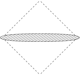
Figure 1: Interior of a Schwarzschild black hole with the quantum region (hatched) replacing the classical singularity. This allows to extend space-time to the new upper region. How these regions are embedded in a full space-time is left unspecified here.

There are many basic aspects which are playing together in just the right way for this result to hold true. They all come directly from the loop quantization and are not put in by hand; in fact, they had been recognized as essential for a background independent quantization a few years before their role in removing classical singularities emerged. The loop representation is important in two ways since via discrete triad spectra it leads to the kinematical results of non-diverging inverse powers of densitized triad components, and through the representation of holonomies to the dynamical constraint as a difference operator. Moreover, the theory is based on densitized triads which, as discussed before, has consequences for the position of classical singularities in minisuperspace important for how one can evolve through them. This automatically provides us with the sign factor from orientation and thus a region beyond the classical singularity. Still, also the dynamical law has to be of the right form for an evolution to this other side of minisuperspace to be possible.

Thus, we have a few essential effects which automatically come from a loop quantization. Once recognized and identified, they can easily be copied in other quantization schemes inspired by loop quantum gravity and cosmology. However, in such a case one has to guess anew in each model what the relevant basic properties would be since there is no underlying scheme for guidance. With the loop quantization we have such a general scheme which just needs to be evaluated in different models. Only then can the results be regarded as reliable expectations for quantum gravity, rather than possibly artificial consequences of choices made. The sign of triad components, for instance, appears automatically and then gives rise to the additional side of the classical singularity to which we can evolve. In loop inspired approaches without a link to the full theory, however, the sign is introduced by hand by extending the range of metric variables to negative values. While this leads to similar results in isotropic models [75], except that the geometrical meaning of the sign remains unclear, there are differences in the black hole interior [76]. In particular, this approach would suggest that even the horizon can be penetrated by the homogeneous quantum evolution despite the fact that space-time becomes inhomogeneous outside. This problem does not occur in the quantization described here since the horizon remains a boundary (corresponding to $\mu=0$).

4.4 Effective dynamics

The non-singular quantum dynamics is obviously very different from the classical one even though they can be shown to agree in classical regions at large densitized triad components and small curvature [77]. In between, there is a regime where equations of motion of the classical type, i.e. ordinary differential equations in coordinate time, should be able to describe the system even though quantum effects are already at work. One can think of these equations as describing the position of wave packets which spread only slightly in semiclassical regimes [45, 46, 47]. Quantum effects will then provide modifications, e.g. where inverse powers of densitized triad components occur in a matter Hamiltonian which are replaced by regular expressions in quantum geometry. This provides different means to calculate implications of quantum effects which can so far be done in homogeneous situations.

For instance if we assume the distribution of a matter system collapsing into a black hole to be isotropic, its outer radius $Ra(t)$ is described by a solution $a(t)$ to the Friedmann equation, with $R$ being the coordinate radius where we cut off spatial slices from a closed FRW model. If we choose a scalar $\phi$ with potential $V(\phi)$ and momentum $p_{\phi}$, we have the Friedmann equation

$$a(\dot{a}^{2}+1)=\frac{8\pi G}{3}({\textstyle\frac{1}{2}}a^{-3}p_{\phi}^{2}+a^{3}V(\phi))$$ (40)

which develops a singularity corresponding to the part of the final black hole singularity covered by matter.

The corresponding effective classical equations are modified by replacing the classically diverging $a^{-3}$ in the matter Hamiltonian with a regular function $d(a)$ derived from finite inverse scale factor operators such as (4.2) [78, 79]. Including two ambiguity parameters $j$ (a half integer) and $0<l<1$, this can be parameterized as

$$d(a)_{j,l}:=a^{-3}p_{l}(3a^{2}/\gamma j\ell_{\rm P}^{2})^{3/(2-2l)}$$ (41)

with

$$p_{l}(q) = \frac{3}{2l}q^{1-l}\left(\frac{1}{l+2}\left((q+1)^{l+2}-|q-1|^{l+2}\right)\right.$$

$$-\left.\frac{1}{l+1}q\left((q+1)^{l+1}-{\rm sgn}(q-1)|q-1|^{l+1}\right)\right)\,.$$

The essential property of $d(a)_{j,l}$ is that it is increasing from zero for $a^{2}<\frac{1}{3}\gamma j\ell_{\mathrm{P}}^{2}$ which through the Friedmann equation implies a different dynamical behavior at small volume. This model then provides an intuitive explanation for the removal of classical singularities even at the effective level since the equations lead to a bounce at non-zero $a$: due to the modified density the kinetic term is negligible at small $a$, and matter evolution equations from the modified matter Hamiltonian imply friction of $\phi$ [80]. The potential term is then dominating and almost constant which means that the bounce is approximately of de Sitter form [52]. In this interpretation of collapsing matter this means that it does not collapse completely but rebounds after a point of minimal contraction is reached.

So far, we had only access to the inside of the matter contribution which we assumed to be isotropic. The solution can now be matched to a suitable solution describing the outside, which would be able to tell us, for instance, whether horizons form. For pressure-less matter one can match to the static Schwarzschild solution as in the Oppenheimer–Snyder model [81]. This is the case classically only for dust, which however can develop pressure if quantum modifications come into play. (This is in agreement with our earlier observations that quantum effects will not allow the presence of a static vacuum solution.) We have thus chosen the more general scalar matter which has pressure even classically. Physically, pressure leads to shock waves at the outer boundary giving rise to a non-static exterior. This can be described by a generalized Vaidya metric

$${\mathrm{d}}s^{2}=-(1-2M(\chi,v)/\chi){\mathrm{d}}v^{2}+2{\mathrm{d}}v{\mathrm{d}}\chi+\chi^{2}{\mathrm{d}}\Omega^{2}$$ (43)

which we can match to the interior (Fig. 2) by requiring equal induced metric and extrinsic curvature at the time-like matching surface $\Sigma$ defined by $r=R$ inside and $\chi=\chi(v)$ outside.

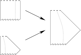
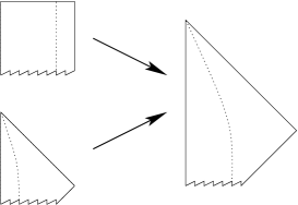
Figure 2: A closed Friedmann–Robertson–Walker model and a generalized Vaidya metric are matched to form a collapse model. Singularities are indicated by dashed lines and the matching surface by dotted lines. The bottom parts of the diagrams are cut off since they depend on details of the solutions. The left hand side shows the classical case with a future singularity, while the right hand side shows the singularity-free effective case.

In this way we can see what the collapsing matter implies for the outside space-time at least in a neighborhood [66]. To have access to the full outside all the way up to an asymptotic observer we would need to specify the matter content outside. While this is possible e.g. as the same scalar matter as inside, only inhomogeneous, it would not necessarily be correct physically. In fact, we have modified only the classical equations describing the interior, while we did not use effective equations outside. When the matter distribution extends over a large region in the early stages, one does not expect strong modifications, but this is not clear close to the bounce. In this region, the interior equations are strongly modified, and this is transferred to the outside via the matching conditions in a rather indirect way: We use the classical generalized Vaidya metric, but did not specify the matter content. It is effectively the energy momentum tensor which carries quantum effects from the interior to the outside via the matching. Prescribing the outside matter content would remove this transfer and stop us from seeing possible quantum effects outside.

We write the interior metric as

$${\mathrm{d}}s^{2}=-{\mathrm{d}}t^{2}+X(r,t)^{2}{\mathrm{d}}r^{2}+Y(r,t)^{2}{\mathrm{d}}\Omega^{2}$$

with $X(r,t)=a(t)/(1+r^{2}/4)$ and $Y(r,t)=rX(r,t)$. On the matching surface $r=R$ of the interior and $\chi=\chi(v)$ of the generalized Vaidya exterior the metric and extrinsic curvature have to agree. From the metrics we obtain

$$\chi|_{\Sigma}=Y|_{\Sigma}$$ (44)

and

$$\left.\frac{{\mathrm{d}}v}{{\mathrm{d}}t}\right|_{\Sigma}=\left.(1-2M/\chi-2{\mathrm{d}}\chi/{\mathrm{d}}v)^{-1/2}\right|_{\Sigma}$$ (45)

while the extrinsic curvature, computed again from (21), gives us

$$\left.\frac{YY^{\prime}}{X}\right|_{\Sigma}=\left.\chi\frac{1-2M/\chi-{\mathrm{d}}\chi/{\mathrm{d}}v}{\sqrt{1-2M/\chi-2{\mathrm{d}}\chi/{\mathrm{d}}v}}\right|_{\Sigma}$$ (46)

and

$$0=\partial_{v}M+\frac{{\mathrm{d}}^{2}\chi}{{\mathrm{d}}v^{2}}+\left(1-\frac{2M}{\chi}-3\frac{{\mathrm{d}}\chi}{{\mathrm{d}}v}\right)\left(\frac{M}{\chi}-\partial_{\chi}M\right)$$ (47)

which yields a condition for $\partial M/\partial\chi$ at constant $v$.

With ${\mathrm{d}}\chi/{\mathrm{d}}v|_{\Sigma}=\dot{\chi}|_{\Sigma}/\dot{v}|_{\Sigma}$ and (44) we use (46) to write the square root in (45) in terms of $Y^{\prime}$ and $\dot{Y}$ which leads to

$$\left.\frac{{\mathrm{d}}v}{{\mathrm{d}}t}\right|_{\Sigma}=\left.\frac{(Y^{\prime}/X+\dot{Y})}{1-2M/Y}\right|_{\Sigma}\,.$$ (48)

Using (44) and defining $c:=Y^{\prime}/X$, (46) becomes

$$c^{2}(1-2M/\chi+2{\mathrm{d}}\chi/{\mathrm{d}}v)=(1-2M/\chi-{\mathrm{d}}\chi/{\mathrm{d}}v)^{2}$$

which with

$$({\mathrm{d}}\chi/{\mathrm{d}}v)^{2}=\dot{Y}^{2}(1-2M/\chi-2{\mathrm{d}}\chi/{\mathrm{d}}v)$$

(following from ${\mathrm{d}}\chi/{\mathrm{d}}v=\dot{\chi}/\dot{v}$ and (45)) gives $c^{2}=1-2M/\chi+\dot{Y}^{2}$. Thus,

$$2M|_{\Sigma}=(Y\dot{Y}^{2}+Y(1-c^{2}))|_{\Sigma}\,.$$ (49)

A trapped surface forms in a generalized Vaidya metric when $2M=\chi$, which lies on the matching surface if $2M=Y$. From (49) this yields the simple condition

$$|\dot{Y}|=c=Y^{\prime}/X$$ (50)

which for FRW reduces to

$$|\dot{a}|=(1-R^{2}/4)/R\,.$$ (51)

Assuming, for now, that this condition will be satisfied at a time $t(R)$ during collapse, we obtain a horizon covering the bounce (Fig. 3). The squared norm of its normal is given by $\partial_{v}M(1-2\partial_{\chi}M)$ which can be computed from (47) using ${\mathrm{d}}M/{\mathrm{d}}v=\partial_{v}M+\partial_{\chi}M{\mathrm{d}}\chi/{\mathrm{d}}v$ and turns out to be zero if the horizon condition (51) is satisfied. The horizon is thus always null when it first intersects the matching surface.

After the first trapped surface forms on the matching surface, $|\dot{a}|$ continues to increase before it turns around when the peak in $d(a)_{j,l}$ is reached. From then on, $|\dot{a}|$ decreases and reaches $\dot{a}=0$ at the bounce. In between, the trapped surface condition (51) will be satisfied a second time at an inner horizon. Unlike the outer one, it lies in the modified regime where energy conditions are effectively violated and $\ddot{a}>0$ [44]. It is also null at the matching surface but can become time-like soon and evaporate later. Similarly, the outer horizon can become time-like when matter having experienced the quantum modifications starts to propagate through it. Thus, also the outer horizon can evaporate and shrink toward the matching surface at later times, when the inner matter is already expanding.

The horizon thus evaporates and the bouncing matter has a chance to reappear. Indeed, the condition (51) will be satisfied also at a time after the bounce where $\dot{a}$ is now positive. Thus, the horizon will intersect again with the matter shells and disappear. At such a point, however, the matching breaks down since ${\mathrm{d}}v/{\mathrm{d}}t$ diverges when $2M=Y$ and $\dot{Y}>0$. From a single matching of the interior we obtain only a part of the collapse before a horizon disappears. At the endpoint of the horizon the interior coordinate $t$ ceases to be good, and we have to match to another patch (Fig. 3).

Figure 3: Sketch of the bouncing effective interior, covered by evaporating horizons (dashed). Constant $v$ (outside) and $t$ (inside) slices are dotted. The matching described in the text only refers to the part before the inner horizon collides with the expanding matter after the bounce.

The precise position of the horizon only follows when we specify the matter content and field equations (i.e. Einstein’s equations or modified ones) and integrate with $M$ and $\partial M/\partial\chi$ as boundary conditions at the matching surface. Since we leave this open, we do not get precise information on the horizon but only qualitative properties. After some time into the collapse, the horizon is expected to shrink since modifications in the interior imply small violations of energy conditions (which also allow the bounce to take place). Radiation of negative energy implies, analogously to Hawking radiation, that the horizon becomes time-like and shrinks. Later, it can meet the matching surface again at which point the matter becomes visible from behind the horizon. If the initial mass was large, it takes a long time for the bounce to occur and the matter to reemerge such that for most of the time the system looks like a classical black hole to an outside observer.

It is not guaranteed that a horizon forms at all since fulfillment of the horizon condition depends on initial values. In particular, once we choose $R$ to specify the matching surface in the interior, Eq. (51) fixes the value for $\dot{a}$ which needs to be reached for a horizon to occur. Classically, $\dot{a}$ is unbounded as we approach the singularity such that the condition will always be true at one point and there is always a horizon covering the classical singularity in this model. With the effective equations, however, $\dot{a}$ is bounded for given initial conditions, and depending on the value of $R$ it can happen that the horizon condition is never fulfilled. In this case, there would not be a black hole but only a matter distribution collapsing to high densities and rebounding. This rules out black holes of a certain type, in particular those of small mass: Starting with a configuration such that a horizon forms, we can decrease $R$ toward zero without changing $a(t)$. The right hand side of (51) then increases and at one point the condition can no longer be fulfilled. Since with decreasing $R$ we carve out a smaller piece of the homogeneous interior, the total initial mass is smaller, giving us a lower bound for the mass of black holes in this model. Precise values have to be derived from more detailed models, but this argument shows that large, astrophysical black holes will be unaffected while primordial ones of small masses do not form [66].

5 Extrapolation

We have seen two results from homogeneous techniques employed in the preceding section:

• At the fully quantum level of the Kantowski–Sachs model describing the Schwarzschild black hole interior the singularity is absent (Fig. 1).

• Matter systems allow effective classical equations for their collapse such that the classical singularity is replaced by a bounce sometimes shrouded by a horizon (Fig. 3).

Both results have been arrived at with very different techniques, and have different physical meaning. The first one only applies to the vacuum case but provides us with a strict result as to how the classical singularity is replaced in quantum gravity. It directly shows that general relativity is singular because it relies on the smooth classical space-time picture. This picture breaks down at high curvature and has to be replaced by discrete quantum geometry, providing a non-singular evolution.

The second result works with matter but is more intuitive, only giving a picture from effective classical equations. It provides a physical, rather than geometrical explanation for the failure of general relativity in strong curvature regimes. Singularities in general relativity can be understood as a consequence of the always attractive nature of classical gravity: Once matter collapses to a sufficiently high density, be it an isolated part or the whole universe, there is nothing to prevent total collapse into a singularity. Viewing the Friedmann equation, e.g. with scalar matter, as describing a mechanics system with the matter energy density serving as potential shows this by the fact that the energy density decreases as a function of $a$ at fixed $\phi$ and $p_{\phi}$, in particular the kinetic term $\frac{1}{2}a^{-3}p_{\phi}^{2}$. Thus, there is an attractive force driving the system toward $a=0$ (or, as usually expressed in cosmology, positive pressure which thermodynamically is defined as the negative change of energy with volume). The modification of $a^{-3}$ by the regular function $d(a)$ in (41), which turns around at a peak value and then approaches zero rather than infinity at $a=0$, implies that now the energy density increases as a function of volume at small scales. This can be interpreted as quantum gravity becoming repulsive at small scales, which can then easily prevent total collapse into a singularity. Moreover, at non-zero but small scales this repulsive component is still active and leads to modified behavior. For instance, in an expanding universe it implies that the expansion is accelerated leading directly to inflation [44]. In the interpretation of collapsing matter, the same effect makes the horizon shrink after the bounce such that only the strong quantum region is covered.

Since we have used approximations, the question arises how these partial results can fit into a full picture of quantum black holes. The first result indicates that space-time can be extended through classical singularities, but since it gives us access only to the interior, it is not clear if the new region we reach can also be accessed from an outside observer. (If not, the black hole would appear as a wormhole through which one can travel into a new region of the universe.) The second result now indicates that we can in fact access the new region since there is only one matching region outside the collapsing matter, suggesting a picture as in Fig. 4. Quite similar ideas have been put forward, by different motivations, in [82, 83, 84].

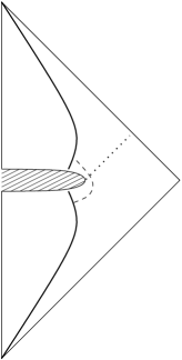
Figure 4: Combination of Figs. 1 and 3 where the quantum region around the classical singularity is shrouded by an evaporating horizon (dashed). The dotted line marks the boundary of the part of space-time unaffected by the strong curvature inside.

However, here it is important to bear in mind that we only effectively described matter outside falling into the collapsing shells. In a more realistic model, there would be such inhomogeneous matter colliding with the homogeneous core and making it more heavy. This can then lead to singularities forming in the outside region. For their resolution we would again have to use quantum geometry and face the same problem as to whether or not this will lead to a new region accessible from the outside.

It is clear that a decisive answer can only be obtained with inhomogeneous techniques, which we are going to describe in the next section. Still, even at this level one can see that there are only a few possible scenarios which can be distinguished by using inhomogeneous properties of quantum geometry. Irrespective of which outcome inhomogeneous models will show us, one can already see special features of quantum geometry leading to a new paradigm about black hole evaporation. For the first time, this takes into account a resolution of the classical singularity with implications for apparent loss of information [68]. In fact, while Hawking radiation still emerges in a neighborhood of the dynamical horizon and is still approximately thermal, this is by no means everything coming out of the black hole at late times. Infalling matter now evolves through the quantum region of high curvature and reappears later, restoring correlations which are not recovered by Hawking radiation alone. In particular, there is no reason for the final state measured on all of future null infinity to be mixed if we started with a pure initial state. In the usual picture one would cut out the quantum region (or the place of the classical singularity) and consider the future space-time without allowing penetration through that region. Future null infinity then stops at the intersection with the dotted line in Fig. 4, and a state retrieved at this part of null infinity is indeed mixed since it is obtained by averaging over the rest to the future. In this way, both the singularity problem and the information loss paradox are resolved by loop quantum gravity.

6 Inhomogeneous techniques

For the spherically symmetric model we need to perform the loop quantization for inhomogeneous configurations (17) and (11) such that the basic fields now depend on the radial coordinate $x$. Instead of using states such as (27) with a finite number of labels, we now have a field theory with infinitely many kinematical degrees of freedom. An orthonormal basis of states is given by [13]

$$\langle A_{x},K_{\varphi}|\ldots,k_{n},\mu_{n},k_{n+1},\mu_{n+1},\ldots\rangle=\prod_{n}\exp({\textstyle\frac{1}{2}}ik_{n}\smallint_{e_{n}}A_{x}{\mathrm{d}}x)\exp(-i\mu_{n}\gamma K_{\varphi}(v_{n}))$$ (52)

with countably many labels $k_{n}\in{\mathbb{Z}}$ and $0\leq\mu_{n}\in{\mathbb{R}}$ labeling edges $e_{n}$ and vertices $v_{n}$, respectively, of a 1-dimensional graph in the radial line. Note that, as already indicated before, we are using exponentials of the extrinsic curvature component $K_{\varphi}$ along homogeneous directions but holonomies of the connection component $A_{x}$ along the inhomogeneous direction. Both exponentials are represented as multiplication operators.

Spatial geometry is encoded in densitized triad operators acting by

$$\hat{E}^{x}(x)|\ldots,k_{n},\mu_{n},\ldots\rangle = \frac{\gamma\ell_{\mathrm{P}}^{2}}{8\pi}\frac{k_{n^{+}(x)}+k_{n^{-}(x)}}{2}|\ldots,k_{n},\mu_{n},\ldots\rangle$$ (53)

$$\int_{\cal I}\hat{E}^{\varphi}|\ldots,k_{n},\mu_{n},\ldots\rangle = \frac{\gamma\ell_{\mathrm{P}}^{2}}{8\pi}\sum_{v_{n}\in{\cal I}}\mu_{n}|\ldots,k_{n},\mu_{n},\ldots\rangle$$ (54)

where $n^{\pm}(x)$ is the edge label to the right (left) of $x$, and ${\cal I}$ is an interval on the radial line (over which we need to integrate $E^{\varphi}$ since it is a density). As before in the homogeneous case we also obtain densely defined operators for inverse powers of the triad components, which can in particular be done for the inverse of $E^{\varphi}$ in the spin connection component (13).

6.1 Hamiltonian constraint

For the Hamiltonian constraint (16) we again have to obtain curvature components from holonomies, now using holonomies of $A_{x}$ for the inhomogeneous radial direction and exponentials of $K_{\varphi}$ for homogeneous directions along symmetry orbits. Terms containing the spin connection component $\Gamma_{\varphi}$ belonging to homogeneous directions will be quantized separately. One may wonder if this procedure will easily give the right components in the Hamiltonian constraint, given that it has the rather simple expression (16) in terms of extrinsic curvature components while we are using the Ashtekar connection component $A_{x}$. As we will see, the general scheme will yield automatically the right combination of components by a straightforward construction of loops to be used in holonomies.

To see this in detail, we first note the difference between $A_{x}$ and $K_{x}$, which is given by the $x$-component of the spin connection. For a general spherically symmetric triad it takes the form

$$\Gamma=-\eta^{\prime}\tau^{3}{\mathrm{d}}x+\frac{E^{x\prime}}{2E^{\varphi}}\Lambda{\mathrm{d}}\vartheta-\frac{E^{x\prime}}{2E^{\varphi}}\bar{\Lambda}\sin\vartheta{\mathrm{d}}\varphi+\tau_{3}\cos\vartheta{\mathrm{d}}\varphi$$ (55)

as in (9) with (10). Here, we recognize (13) as used before as the component along homogeneous directions. This component is a scalar (noting that both $E^{x\prime}$ and $E^{\varphi}$ are densities of weight one), while the $x$-component $\Gamma_{x}=-\eta^{\prime}$ does not have covariant meaning and indeed can be made arbitrarily small locally by a suitable gauge transformation. This is analogous to the situation in the full theory, while the gauge invariant meaning of $\Gamma_{\varphi}$ mimics homogeneous models.

Even though $\Gamma_{x}$ can be made arbitrarily small locally by a gauge transformation, we cannot assume this when constructing a suitable Hamiltonian constraint operator. Thus, it must be built into the construction so as to combine with $A_{x}$ from radial holonomies to give $K_{x}$ as in the expression for the constraint. This $K_{\varphi}K_{x}$-term in the constraint can, according to the general construction where connection or extrinsic curvature components derive from closed holonomies, only come from a loop which has one edge along a symmetry orbit and one in the radial direction. Starting in a point $v$, such a holonomy is of the form $h_{x}^{(\delta_{x})}h_{\varphi}^{(\delta)}(v_{+})(h_{x}^{(\delta_{x})})^{-1}(h_{\varphi}^{(\delta)}(v))^{-1}$ with a new vertex $v_{+}$ displaced from $v$ by a coordinate distance $\delta_{x}$ of the radial edge. (We distinguish between $\delta_{x}$ for the radial direction and $\delta$ for the angular directions since the continuum limit is technically different in both cases.) This term appears together with $\bar{\Lambda}(v)$ (coming from quantizing the triad components) in a trace whose expansion in $\delta$

$$-2\mathop{\mathrm{tr}}(h_{x}h_{\varphi}(v_{+})h_{x}^{-1}h_{\varphi}(v)^{-1}\bar{\Lambda}(v))$$

$$\quad\sim-2\gamma\delta(K_{\varphi}(v_{+})\mathop{\mathrm{tr}}(\Lambda(v_{+})\bar{\Lambda}(v))+2K_{\varphi}(v_{+})\smallint A_{x}{\mathrm{d}}x\mathop{\mathrm{tr}}(\tau_{3}\Lambda(v_{+})\bar{\Lambda}(v)))$$

$$\quad=\gamma\delta(K_{\varphi}(v_{+})\sin(\eta_{+}-\eta)+K_{\varphi}(v_{+})\smallint A_{x}{\mathrm{d}}x\cos(\eta_{+}-\eta))$$

$$\quad=\delta\delta_{x}\gamma K_{\varphi}(v)(A_{x}(v)+\eta^{\prime}(v))+O(\delta^{2})$$ (56)

has all the right terms, with $A_{x}$ coming directly from the radial holonomy and $\eta(v_{+})$ in $\delta\eta^{\prime}\sim\eta(v_{+})-\eta(v)$ from the internal direction $\Lambda(v_{+})$ at the new vertex. The other term of the form $K_{\varphi}^{2}$ is obtained from angular holonomies only, as in the homogeneous case,

$$-2\mathop{\mathrm{tr}}(h_{\vartheta}h_{\varphi}h_{\vartheta}^{-1}h_{\varphi}^{-1}\tau_{3})\sim\delta^{2}\gamma^{2}K_{\varphi}^{2}\,.$$ (57)

The matrices $\tau_{3}$ and $\bar{\Lambda}(v)$ in the traces come from Poisson brackets expressing triad components as in the homogeneous constraint. Moreover, the spin connection components in (16) are again expressed through the curvature

$$F(\Gamma)=-\Gamma_{\varphi}^{\prime}\Lambda{\mathrm{d}}x\wedge{\mathrm{d}}\vartheta+\Gamma_{\varphi}^{\prime}\bar{\Lambda}\sin\vartheta{\mathrm{d}}x\wedge{\mathrm{d}}\varphi+(\Gamma_{\varphi}^{2}-1)\tau_{3}\sin\vartheta{\mathrm{d}}\vartheta\wedge{\mathrm{d}}\varphi$$

of the spin connection. Through

$$\sum_{IJK}\epsilon^{IJK}\mathop{\mathrm{tr}}(\delta_{I}\delta_{J}F(\Gamma)_{IJ}h_{K}\{h_{K}^{-1},V\})\propto(\Gamma_{\varphi}^{2}-1)\{A_{x},V\}-2\Gamma_{\varphi}^{\prime}\{-\gamma K_{\varphi},V\})$$

we obtain the additional terms of the constraint, where we included the length parameters $\delta_{I}$ (i.e. $\delta_{x}$ for $I=x$ and $\delta$ for $\vartheta$ or $\varphi$).

This demonstrates how the general procedure works without additional input: We use exponentials of extrinsic curvature components for homogeneous directions and holonomies of Ashtekar connection components for inhomogeneous ones as dictated by the background independent representation. Spin connection components for inhomogeneous directions then come in the right form to combine with extrinsic curvature components, while those in homogeneous directions are split off and quantized separately. This is possible because those components, in contrast to the inhomogeneous ones, do have covariant meaning. This ties together the constructions in homogeneous models and the full theory, and at the same time opens a direct route to effective classical equations: Homogeneous spin connection components usually contain inverse powers of the densitized triad, such as (13). When they are quantized, the classical divergence will be removed implying modifications at small scales. in homogeneous models this has been used, e.g., in the Bianchi IX case where it has been shown to remove the classical chaos [85, 86]. Similarly, one can use this mechanism to derive effective classical equations for the spherically symmetric model and find possible consequences.

Before trusting those effective equations in the inhomogeneous case one needs to make sure that there is a well-defined Hamiltonian constraint operator emerging from the procedure described here. So far, we have only discussed those holonomies and spin connection components which give us the contributions to the constraint, but they must now be stuck together with quantizations of triad components so as to build a well-defined operator for the whole expression. Moreover, since the expression (16) is an integrated density, one has to discretize the integration first and then, after quantizing the individual terms, perform the continuum limit removing the regulator. The discretization had already been understood above, with $v$ and $v_{+}$ being the endpoints of a discrete interval of size $\delta_{x}$, and we convinced ourselves that the continuum limit of the discretization will yield the correct result. In more detail, one writes

$$H[N]=\int{\mathrm{d}}xN(x){\cal H}(x)\sim\sum_{n}\delta_{x}^{(n)}N(v_{n}){\cal H}(v_{n})$$

where we discretized the radial line into intervals of coordinate length $\delta_{x}^{(n)}$, each one containing the point $v_{n}$. Classically, both expressions can be made to agree for any subdivision by choosing points $v_{n}$ in the intervals according to the mid point theorem. Alternatively, if one wants to fix the $v_{n}$ to be endpoints of the intervals, the discretization agrees with the classical constraint in the continuum limit in which $n\to\infty$ and $\delta_{x}^{(n)}\to 0$ for all $n$.

For the Hamiltonian constraint in general each term in the sum then has contributions of the form

$$\delta_{x}{\cal H}(v)\propto\sum_{I,J,K}\epsilon^{IJK}\mathop{\mathrm{tr}}(h_{IJ}h_{K}[h_{K}^{-1},\hat{V}])$$ (58)

where we sum over triples $(I,J,K)$ of independent directions which in symmetric models are given by generators of the symmetry transformations ($(\vartheta,\varphi)$ in the spherically symmetric case), and in the full theory or inhomogeneous directions of a symmetric model by edges of a graph ($x$ in spherical symmetry). The holonomies $h_{IJ}$ are formed according to the symmetry: if both directions $I$ and $J$ are inhomogeneous, $h_{IJ}$ is a holonomy along a closed loop $\alpha_{IJ}$ constructed from edges in the $IJ$-plane of a graph to act on; if at least one of the two directions is homogeneous, $h_{IJ}=h_{I}h_{J}h_{I}^{-1}h_{J}^{-1}-\gamma^{2}\delta_{I}\delta_{J}\hat{F}_{IJ}$ with $h_{I}$ being exponentials of the (su(2)-valued) extrinsic curvature components belonging to the $I$-direction for a homogeneous direction $I$ or holonomies along an inhomogeneous direction. (The appearance of $F(\Gamma)$ can be understood as a correction term since loops made from holonomies along vector fields generating symmetries do not close if orbits have non-zero curvature [87].) The size of loops $\alpha_{IJ}$ or single holonomies is determined by the size $\delta_{x}$ of the discretization. The final holonomy $h_{K}$ either belongs to an edge transversal to both directions $I$ and $J$, or again to exponentiated extrinsic curvature components if $K$ is homogeneous. These combinations are chosen in such a way that $h_{IJ}$ yields the correct curvature components, the commutator gives the necessary triad components, and both terms together provide just the right product of lattice sizes such as $\delta_{x}$ in order for the sum to take the form of a Riemann summation of the original integral. In the full theory, this procedure only results in the so-called Euclidean part of the constraint which can be used to construct the Lorentzian constraint [71]. In the models used here, however, the prescription (58) is sufficient even for Lorentzian signature.

This can now be illustrated and applied in the spherically symmetric model where the first case above cannot appear since there is only one inhomogeneous direction. We have thus two cases, one in which direction $I$ or $J$ is radial, resulting in the first product of holonomies discussed above, combined with a commutator

$$h_{\varphi}[h_{\varphi}^{-1},\hat{V}] = \hat{V}-\cos{\textstyle\frac{1}{2}}\gamma K_{\varphi}\hat{V}\cos{\textstyle\frac{1}{2}}\gamma K_{\varphi}-\sin{\textstyle\frac{1}{2}}\gamma K_{\varphi}\hat{V}\sin{\textstyle\frac{1}{2}}\gamma K_{\varphi}$$

$$-2\Lambda(\cos{\textstyle\frac{1}{2}}\gamma K_{\varphi}\hat{V}\sin{\textstyle\frac{1}{2}}\gamma K_{\varphi}-\sin{\textstyle\frac{1}{2}}\gamma K_{\varphi}\hat{V}\cos{\textstyle\frac{1}{2}}\gamma K_{\varphi})\,.$$

In the second case we have the other product of holonomies and a commutator

$$h_{x}[h_{x}^{-1},\hat{V}] = \hat{V}-\cos{\textstyle\frac{1}{2}}\smallint A_{x}\hat{V}\cos{\textstyle\frac{1}{2}}\smallint A_{x}-\sin{\textstyle\frac{1}{2}}\smallint A_{x}\hat{V}\sin{\textstyle\frac{1}{2}}\smallint A_{x}$$

$$+2\tau_{3}(\cos{\textstyle\frac{1}{2}}\smallint A_{x}\hat{V}\sin{\textstyle\frac{1}{2}}\smallint A_{x}-\sin{\textstyle\frac{1}{2}}\smallint A_{x}\hat{V}\cos{\textstyle\frac{1}{2}}\smallint A_{x})\,.$$

The integration here is over an interval of size $\delta_{x}$ such that in the limit of a fine discretization this term is of order $\delta_{x}$ as needed for the Riemann sum.

What we did not specify yet is how the discretization is adapted to a graph the constructed operator is supposed to act on, i.e. whether $v$ and maybe $v_{\pm}$ are already vertices of the graph or arbitrary points. At this point, choices need to be made which lead to different versions of the constraint. The same choices arise in the full theory [88, 89, 90], but they can be studied much more easily in the spherically symmetric model such that it may be possible to rule out some versions.

It is already non-trivial to check that different versions lead to well-defined operators at all. For this, the action after performing the continuum limit, in which the number of discretization points becomes infinite, must be finite. If the action were non-zero at each discretization point, there would not be a well-defined operator in the limit and the regulator could not be removed. One would then only deal with a lattice regulated theory rather than a quantization of the continuum theory. In the full theory, there is a well-defined operator because the action of the constraint is zero unless a discretization point is already a vertex. Starting with states with finitely many vertices then leads to a densely defined operator. This comes about in the full theory because the constraint contains the volume operator in such a way that it acts only on planar vertices if there is no vertex already present in the graph. Since the full volume operator annihilates all planar vertices, there are only finitely many contributions from the vertices already present.

In spherical symmetry, however, all vertices are planar since graphs are just 1-dimensional. This simple general argument is thus not available and it is not obvious that the same construction scheme will result in a well-defined operator. It turns out, however, that this is the case as a consequence of how triad components in the constraint are quantized: a discretization point which is not already a vertex of the graph to act on will be annihilated such that only finitely many contributions from the vertices remain. One can thus use the same type of operator, just with adaptations to the symmetric situation.

Nevertheless, one can also choose different constructions where the discretization is given directly by the graph, i.e. discretization intervals would be complete edges of the graph. Since endpoints of discretization intervals are always vertices of a state, the continuum limit would then require also states to change and become finer and finer. In this picture, the continuum limit of the constraint operator can only be tested on states which are suited to the continuum behavior, while there are also other states where discreteness is essential and where the classical constraint would be corrected from quantum effects. Moreover, in the continuum limit the number of vertices diverges and the constraint operator becomes ill-defined just as the usual Wheeler–DeWitt operator is. Both schemes result in well-defined operators, but they lead to quite different equations of motion and require different conceptual viewpoints about the continuum limit. When the continuum limit is to be ensured for each state, one requires in a sense that the classical equations are sensible at arbitrarily small scales, and corrections could only come from quantum uncertainties. In the second picture, on the other hand, the classical continuum picture arises only after a certain coarse graining, or by working only with states which are not sensitive to the microscopic structure. If one chooses a state which is sensitive to small scales, or looks very closely at small scales of even a semiclassical state, then corrections to the classical expressions arise, for instance as a consequence of the underlying discreteness. This second viewpoint has been taken successfully in cosmological models, and is, as we will see, also fruitful in black hole models.

6.2 Dynamics

Since the constraint operator is again constructed from holonomies which act by shifting the labels, it implies difference equations for states in a triad representation. (Note that also in the spherically symmetric model the triad representation exists, unlike in the full theory where flux operators do not commute [91].) These equations are now not only partial difference equations but also have many independent variables. Interestingly, the type of difference equation is very different for the two versions of the constraint operator: in the second case the number of edges and vertices of the original state is unchanged and the operator only acts on the labels. This results in difference equations with independent variables $k_{e}$ for each edge and $\mu_{v}$ for each vertex. Since the operator does not change the number of edges and vertices, one obtains coupled difference equations in a fixed number of variables for each sector given by the number of vertices.

In the first version of the constraint, however, the situation is very different. Now, new vertices are created and edges split in each action of the operator. Thus, for a triad representation it is not enough to work with a fixed number of vertices. Rather, all graphs have to be taken into account for the equation, which implies that one has to deal with infinitely many independent variables and thus functional difference equations.

We thus return to the simpler type of difference equation implied by the other version of the constraint and discuss what one can already say about the singularity issue. First of all, one will have to identify classical singularities on minisuperspace in order to study the constraint equation in a neighborhood. In an isotropic model this is simple since the only way is for the volume to go to zero [10]. Similarly, one can identify the classical singularity on an anisotropic minisuperspace where all densitized triad components would go to zero. The situation is not so clear in midisuperspaces such as spherical symmetry since there are more possibilities for a singularity to develop. Even though this has not been settled in general, there are many cases where a singularity is characterized by $E^{x}$ approaching zero (which on classical solutions such as Schwarzschild implies that $E^{\varphi}$ becomes zero, too). This is also in agreement with the general mechanism removing singularities seen so far in homogeneous models: there it is the sign coming from orientation which leads to different regions of minisuperspace separated by the classical singularity. The quantum evolution, as we have seen in the Kantowski–Sachs model, can then allow us to evolve between the two regions, thus removing the classical singularity as a boundary.

The role of orientation is now played by $\mathop{\mathrm{sgn}}E^{x}$ since $\det q=E^{x}(E^{\varphi})^{2}$. Since $E^{x}$ depends on the radial position, or the edge after quantization, the boundary of our midisuperspace has many components which we can identify with an inhomogeneous classical singularity, corresponding to the fact that inhomogeneous singularities behave differently in their different points. For the states this means that we encounter a section of a classical singularity each time an edge label $k_{e}$ becomes zero. As in homogeneous models, we can then use the evolution equation in the triad representation in order to see if an evolution through this part of the boundary is possible. Since the structure of the difference equation for a given edge label is very similar to the homogeneous equation, one can expect that the boundary indeed disappears and that the quantum evolution connects regions of midisuperspace corresponding to different local orientations. There would thus be no singular boundary, and the same mechanism as in homogeneous models could also remove spherically symmetric singularities.

This scenario has been verified in [15], noting a crucial difference to homogeneous models wich require a symmetric ordering of the constraint. Thus, quantization choices are reduced by looking at less symmetric models, so far in such a way which maintains the validity of the general picture. Yet, there are also open issues left for a general understanding. For instance, while the results are independent of the matter Hamiltonian and can be extended to cylindrical gravitational wave models, thus also allowing local degrees of freedom, they are so far based only one type of the constraint which leads to difference equations easier to deal with. The behavior with the other version is not easy to see, but if it is singularity free, too, the mechanism is likely to be different. Most importantly, the kind of initial/boundary value problem suitable for the constraint equations needs to be analyzed in more detail to guarantee that there are suitable and sufficiently many solutions with the correct classical limit. At this point the anomaly issue, i.e. whether two constraint operators with different lapse functions have the correct commutator, becomes important. These considerations thus provide a promising and treatable way to distinguish different versions of the quantization by their physical implications, which can then be extrapolated to the full theory.

6.3 Horizons

A feature of black holes which is new compared to cosmological models, and which requires inhomogeneous situations, is given by the presence of horizons. Global concepts such as the event horizon are, of course, not helpful in our case since we would need to solve the Hamiltonian constraint completely before being able to discuss this issue. There are more practical definitions such as apparent horizons which, however, are much more general and do not distinguish between fully dynamical situations and almost static systems. The quantum behavior would be most easy to analyze if we can define horizons locally and in a controlled manner which does not require the full dynamics at once. Such a concept is presented by isolated [2] or slowly evolving dynamical horizons [92], which even quite unexpectedly simplify the spherically symmetric Hamiltonian constraint in their neighborhood.

6.3.1 Definition

There are three main parts to the definition of an isolated horizon $\Delta$ with spatial sections $S\cong S^{2}$ of given area $a_{0}$, embedded into the space manifold $\Sigma$ by $\iota\colon S\to\Sigma$ [93, 30]:

1. The canonical fields $(A_{a}^{i},E^{a}_{i})$ on the horizon are completely described by a single field $W=\frac{1}{2}\iota^{*}A^{i}r_{i}$ on $S$ which is a U(1)-connection obtained from the pull-back of the Ashtekar connection to $S$. Here, $r_{i}$ is an internal direction on the horizon chosen such that $W$ is a connection in the spin bundle on $S^{2}$ and $r^{i}E_{i}^{a}=\sqrt{\det q}\,r^{a}$ on the horizon with the internal metric $q$ on $S$ and the outward normal $r^{a}$ to $S$ in $\Sigma$.

2. The intrinsic horizon geometry, given by the pull-back of the 2-form $\Sigma^{i}_{ab}:=\epsilon_{abc}E^{c}_{i}$ to $S$, is determined by the curvature $F={\mathrm{d}}W$ of $W$ by

   $$F=-\frac{2\pi}{a_{0}}\iota^{*}\Sigma^{i}r_{i}\,.$$ (59)

3. The constraints hold on $S$.

A further consequence of the isolated horizon conditions [93] is that the curvature ${\cal F}$ of the pull-back of $A_{a}^{i}$ to $S$ has to equal the curvature of $W$: $r_{i}{\cal F}(\iota^{*}A^{i})=2{\mathrm{d}}W$. This can be seen as one of the distinguishing features of an isolated horizon since even slowly evolving horizons at rate $\epsilon$ (related to the expansion of horizon cross sections [92]) will break it, though just by an amount of the order $\epsilon^{2}$.

When the horizon is introduced as a boundary, condition (i) is used to identify the horizon degrees of freedom represented by the field $W$. Condition (ii) then shows that these degrees of freedom are fields of a Chern–Simons theory on the horizon. It is the main condition since it relates the horizon degrees of freedom to the bulk geometry, which after quantization selects the relevant quantum states to be counted. Condition (iii), on the other hand, does not play a big role since an isolated horizon as boundary implies a vanishing lapse function on $S$ for the Hamiltonian constraint which then is to be imposed only in the bulk.

Thus, when computing black hole entropy in this way, as we will describe later, the Hamiltonian constraint does not play any role since it does not act at the boundary, and the Hamiltonian generating evolution along the horizon need not be considered. In the spherically symmetric model one can hope that the constraint is simple enough for an application in this case, either to generate evolution or to impose the horizon not as a boundary but inside space such that the constraint would have to be imposed. In the latter case, moreover, we will not be able to have an independent boundary theory which is then matched to the bulk, but would have to find the relevant degrees of freedom within the original quantum theory.

6.3.2 Spherical symmetry

We can now evaluate the conditions for spherically symmetric connections of the form

$$A = A_{x}(x)\tau_{3}{\mathrm{d}}x+A_{\varphi}(x)\bar{\Lambda}^{A}(x){\mathrm{d}}\vartheta+A_{\varphi}(x)\Lambda^{A}(x)\sin\vartheta{\mathrm{d}}\varphi+\tau_{3}\cos\vartheta{\mathrm{d}}\varphi$$ (60)

and densitized triads (11), where in general the internal directions $\Lambda^{A}$ and $\Lambda$ are different. The connection component $A_{x}$ has been discussed before, while the relation $A_{\varphi}\Lambda^{A}=\Gamma_{\varphi}\bar{\Lambda}-\gamma K_{\varphi}\Lambda$, following from the definition of the Ashtekar connection together with (9), (10) and (17), implies $A_{\varphi}^{2}=\Gamma_{\varphi}^{2}+\gamma^{2}K_{\varphi}^{2}$.

We choose $r_{i}:=\mathop{\mathrm{sgn}}(E^{x})\delta_{i,3}$ such that in fact $r^{i}E^{a}_{i}=|E^{x}|\sin\vartheta\partial_{x}$ with the intrinsic horizon area element $|E^{x}|\sin\vartheta$ of a metric $|E^{x}|{\mathrm{d}}\Omega^{2}$. Thus, $W=\frac{1}{2}r_{i}\iota^{*}A^{i}=\frac{1}{2}\mathop{\mathrm{sgn}}(E^{x})\cos\vartheta{\mathrm{d}}\varphi$ whose integrated curvature given by $\oint_{S}{\mathrm{d}}W=-2\pi\mathop{\mathrm{sgn}}(E^{x}(x))$ agrees with the Chern number of the spin bundle, depending on the orientation given by $\mathop{\mathrm{sgn}}(E^{x})$.

Evaluating (59) first shows that in the spherically symmetric context it is not restrictive since we have $a_{0}=4\pi|E^{x}(S)|$ and the right hand side given by $-\frac{1}{2}\mathop{\mathrm{sgn}}(E^{x}(S))$ equals $F$ for all $E$. This is not surprising since the spherically symmetric intrinsic geometry of $S$ is already given by the total area which is fixed from the outset. (What is free is the sign of $E^{x}(S)$, or orientation, which confirms ideas of [94].) Now the first condition plays a major role, which we evaluate in the form $r_{i}{\cal F}(\iota^{*}A^{i})=2{\mathrm{d}}W$ [93]. Since ${\cal F}(\iota^{*}A)=(A_{\varphi}^{2}-1)\tau_{3}\sin\vartheta{\mathrm{d}}\vartheta\wedge{\mathrm{d}}\varphi$, the condition requires $A_{\varphi}=0$ which will be the main restriction we have to impose on quantum states in addition to the constraints. This condition $A_{\varphi}=0$ selects 2-spheres in a spherically symmetric space-time corresponding to cross-sections of a horizon. Indeed, for the Schwarzschild solution we have $A_{\varphi}=\Gamma_{\varphi}$ since the extrinsic curvature vanishes. With (13) and the Schwarzschild triad we obtain the correct condition $x=2M$ for the horizon. In general, $A_{\varphi}^{2}=\Gamma_{\varphi}^{2}+\gamma^{2}K_{\varphi}^{2}=0$ implies $\Gamma_{\varphi}=0$ and $K_{\varphi}=0$.

A slowly evolving horizon at rate $\epsilon$ satisfies the condition $r_{i}{\cal F}(\iota^{*}A^{i})=2{\mathrm{d}}W$ only up to terms of the order $\epsilon^{2}$. Thus, $A_{\varphi}$ is not exactly zero but must be small of order $\epsilon$, which then is true also for $\Gamma_{\varphi}$ and $K_{\varphi}$.

6.3.3 Dynamics

In spherical symmetry we can locate a horizon on a state [69], which must be at a vertex in order for $K_{\varphi}=0$ to be sharp enough. The condition that $K_{\varphi}$ be zero for an isolated horizon or small for a slowly evolving horizon then leads to important simplifications which allow a perturbative treatment of the dynamics around the horizon. Indeed, when acting with the constraint at the horizon both terms made from holonomies $h_{IJ}$ contain factors of $\sin\frac{1}{2}\gamma K_{\varphi}$ at the horizon vertex or a neighboring one which must then be small. Ignoring those terms in an approximation leads to an operator which is diagonal on the spin network states (52) and thus easy to solve as a constraint or to use for generating time evolution at a boundary. The additional terms ignored in this approximation can then be included in a perturbative treatment of the near horizon dynamics.

Without many calculations this already shows how the horizon fluctuates dynamically. Classically an isolated horizon has constant area which thus commutes with the Hamiltonian constraint. This is also true at the quantum level to leading order of the above approximation since the area operator $\hat{A}(S)=4\pi|\hat{E}^{x}(S)|$ has the same eigenstates (52) as the leading order constraint. Thus, at this level the horizon area is an observable not just when the horizon is treated as a boundary, but also if its full neighborhood is quantized. However, there are additional terms which arise in higher orders of the perturbation scheme. There are two reasons for horizon area fluctuations even in the isolated case: While classically $K_{\varphi}=0$ exactly at the horizon and only this value is important, the quantization does not allow this to hold arbitrarily sharply. Otherwise, the volume of a shell around the horizon, which depends on the conjugate momentum $E^{\varphi}$ of $K_{\varphi}$ could not be sharp independently of the mass which would contradict semiclassical properties to hold true at least for massive black holes. Secondly, the constraint operator acting at the horizon itself depends on neighboring values of $K_{\varphi}$ through $h_{\varphi}(v_{+})$ in (6.1). This would give non-zero contributions even if $K_{\varphi}$ at the horizon would be zero exactly.

Both terms lead to small dynamical changes in the horizon area coming from typical quantum gravity properties. The first reason is quantum uncertainty which does not allow a sharp condition $K_{\varphi}=0$, and the second space-discreteness and non-locality which implies that not only $K_{\varphi}$ at the horizon itself is relevant but also the values in neighboring vertices which are not necessarily zero. For large black holes, the correction terms are expected to be small: uncertainty will not change the horizon area much compared to its already large size, and in neighboring vertices of a semiclassical state $K_{\varphi}$ will still be extremely small. Thus, for large black holes the horizon area is an excellent observable, while for microscopic black holes large fluctuations are expected which may even prevent horizons as they are known classically. This agrees with the picture we have obtained from effective equations and matching techniques before.

7 Full theory

The methods developed so far in symmetric models mimic those of the full theory, with some adaptations to preserve the symmetry. In this section, for completeness, we describe what this looks like in the full theory and discuss applications which work without assuming symmetries.

7.1 Representation

As discussed before, the full theory of loop quantum gravity is based on holonomies for arbitrary edges in space and fluxes for surfaces, forming the basic classical Poisson algebra. In the connection representation, states are functionals on the infinite dimensional space of connections [95, 96, 70] through holonomies, and a dense subspace of the Hilbert space is spanned by cylindrical functions

$$\psi(A)=f_{\gamma}(h_{e_{1}}(A),\ldots,h_{e_{n}}(A))$$ (61)

which depend on only finitely many holonomies. Since there is now no symmetry requirement, the edges can be arbitrary curves in space and form a graph $\gamma$ with vertices at their intersection points. The inner product for two states associated with the same graph is given by

$$\langle f_{\gamma}|g_{\gamma}\rangle=\int_{SU(2)^{n}}\prod_{e\in\gamma}{\rm d}\mu_{H}(h_{e})f_{\gamma}(h_{1},\ldots,h_{n})^{*}g_{\gamma}(h_{1},\ldots,h_{n})$$ (62)

with the Haar measure ${\mathrm{d}}\mu_{H}$ on the structure group SU(2). For two functions with different graphs, they need to be extended to a bigger one which is always possible by cutting edges or inserting new ones on which the extended state depends trivially. An orthonormal basis is given by spin network states [97, 98], associated with graphs labeled by irreducible SU(2) representations $j_{e}$ at edges and contraction matrices $C_{v}$ at vertices, of the form

$$T_{\gamma,j,C}(A)=\prod_{v\in\gamma}C_{v}\cdot\prod_{e\in\gamma}\rho_{j_{e}}(h_{e}(A))$$ (63)

where the representation matrices $\rho_{j_{e}}(h_{e}(A))$ evaluated in edge holonomies are multiplied together in vertices according to the symbols $C_{v}$.

Fluxes are quantized as derivative operators in the connection representation since the densitized triad is conjugate to the Ashtekar connection. Replacing the triad components in (15) by functional derivatives and acting on a cylindrical function, we obtain

$$\hat{F}_{S}f_{\gamma} = -8\pi i\gamma\hbar G\int_{S}{\rm d}^{2}y\tau^{i}n_{a}\frac{\delta}{\delta A_{a}^{i}(y)}f_{\gamma}(h(A))$$

$$= -i\gamma\ell_{\mathrm{P}}^{2}\sum_{e\in\gamma}\int_{S}{\rm d}^{2}y\tau^{i}n_{a}\frac{\delta h_{e}}{\delta A_{a}^{i}(y)}\frac{{\mathrm{d}}f_{\gamma}(h)}{{\mathrm{d}}h_{e}}$$

which has contributions only from intersection points $y$ of the surface $S$ of the flux with the graph $\gamma$ associated with the state. Moreover, each derivative operator for an intersection point can be seen to be equivalent to an angular momentum operator such that its spectrum is discrete and equidistant. Since there is a finite sum over all such contributions, the spectrum of flux operators is discrete, too. Not all the angular momentum operators involved necessarily commute, and so triad operators do not always commute with each other such that a triad representation does not exist [91] (unlike in the symmetric models studied before).

The densitized triad describes spatial geometry, and spatial quantum geometry is encoded in flux operators. From the basic ones one can construct geometrical operators such as the area [32, 33] or volume operator [34] which also have discrete spectra. Thus, quantum spatial geometry is discrete in a precise way, given by the spectra of geometric operators. The area spectrum is known completely, but for the volume operator this is impossible to compute explicitly since arbitrarily large matrices would have to be diagonalized. Spatial geometry at the quantum level is thus rather complicated in general if explicit calculations need to be done.

This translates to the Hamiltonian constraint and other operators, for which the volume operator plays a crucial role. Classically, the Hamiltonian constraint is given by [21]

$$H[N]=(8\pi G)^{-1}\int{\mathrm{d}}^{3}xN(x)|\det E|^{-1/2}(F_{ab}^{i}E^{a}_{j}E^{b}_{k}\epsilon_{ijk}-2(1+\gamma^{2})K_{[a}^{i}K_{b]}^{j}E_{i}^{a}E_{b}^{k})$$ (64)

with the curvature $F_{ab}^{i}$ of the Ashtekar connection, and the extrinsic curvature $K_{a}^{i}=\gamma^{-1}(\Gamma_{a}^{i}-A_{a}^{i})$ a function of the basic variables through (6). Both parts of the constraint can be quantized using building blocks similar to (58), resulting in a well-defined operator [71] even when matter Hamiltonians are included [37]. Edges for the holonomies have to be chosen, which can be done in a diffeomorphism invariant manner and even in such a way that the quantization is anomaly free at least on states satisfying the diffeomorphism constraint [99].

Which version of the quantization is the correct one, however, is still an open issue since in particular the classical limit and that of perturbations on a classical background (“gravitons”) are difficult to analyze. Moreover, finding and interpreting solutions in full generality is complicated by technical and conceptual problems.

It is thus important to devise approximation schemes, other than symmetry reduction as employed before, in order to shed light on physical properties of the full theory. One powerful possibility consists in imposing an isolated horizon as a boundary [93] since boundary conditions imply that the constraint is not to be imposed there (a constraint has lapse function going to zero at the isolated horizon). Thus, also at the quantum level the constraint operator can be ignored and aspects of the basic quantum representation receive physical meaning. Indeed, boundary degrees of freedom are obtained from intersections of spin network states with the horizon surface, and flux operators are important to select physical states corresponding to an isolated horizon. By counting those states and comparing with the Bekenstein–Hawking expectation the theory can be tested.

7.2 Black hole entropy

An isolated horizon $S$ with prescribed area $a_{0}$ as a boundary leads to an additional boundary term in the symplectic structure [93],

$$\Omega=(8\pi\gamma G)^{-1}\int{\mathrm{d}}^{3}x\partial A_{a}^{i}\wedge\partial E^{a}_{i}+\frac{a_{0}}{2\pi}(16\pi\gamma G)^{-1}\int_{S}{\mathrm{d}}^{2}yr_{i}r_{j}\partial A_{a}^{i}\wedge\partial A_{b}^{j}\epsilon^{ab}$$ (65)

where we denote differentials on field space by $\partial$, $\epsilon^{ab}$ is the anti-symmetric tensor on the boundary surface, and $r_{i}$ the internal vector as in the definition of an isolated horizon. The boundary term to the symplectic structure can be recognized as that of a U(1) Chern–Simons theory which thus describes the horizon degrees of freedom by the U(1) connection $W_{a}=\frac{1}{2}r_{i}A_{a}^{i}$.

We quantize the full system by using quantum geometry in the bulk and quantum Chern–Simons theory on the horizon. Doing this results in the curvature $F={\mathrm{d}}W$ becoming an operator with equidistant spectrum which, via (59) needs to be matched to the flux $r_{i}\Sigma^{i}$ through the horizon. As shown before, quantum geometry indeed implies a flux operator with equidistant spectrum such that the matching is possible at the quantum level. Since also the pre-factors match, there are always solutions to the horizon condition which can now be counted, for a given area $a_{0}$, to compute the entropy as the logarithm of the number of states.

This results in an expression for entropy which is proportional to the horizon area [7, 8], confirming expectations from semiclassical considerations. Intuitively, entropy counts the number of ways that one can construct a macroscopic horizon of area $a_{0}$ from elementary discrete parts [100] (which is generalized in this picture since there is not just one elementary type but different ones given by the spin label of an intersection point with a spin network). Since the discreteness scale is set by the Barbero–Immirzi parameter $\gamma$, the number of possible such configurations and thus entropy must depend on $\gamma$. Indeed, $\gamma$ appears in the constant of proportionality between entropy and area which allows us to fix $\gamma$ by requiring the Bekenstein–Hawking law. Moreover, since there are different types of black holes — charged, distorted, rotating or with non-standard matter couplings — and the value is already fixed by the simplest case of a Schwarzschild black hole, one can test the theory since now entropy must result in the right way without any further parameter to tune. This is indeed the case [101, 102], providing a non-trivial test of the theory.

The scale of discreteness is then fixed which, since it must be small enough, can already be confronted with observations. It turns out that $\gamma=0.2735$ [103, 104] is of the order one such that the discreteness lies around $\sqrt{\gamma}\ell_{\mathrm{P}}\approx\frac{1}{2}\ell_{\mathrm{P}}$ and is thus much too small to be observable directly. Indeed there have long been reasons to expect a scale of discreteness around the Planck length which is now confirmed by detailed calculations in loop quantum gravity. It is not at all obvious that this comes about since there are many non-trivial steps in the derivation, and mistakes in the foundations of the theory could easily lead to larger values which could already be in conflict with observations.

At this point it is important to consider the physical meaning of $\gamma$. It can be seen as a fundamental parameter setting the scale of discreteness which is thus characteristic of quantum gravity. (In fact, one can express the continuum limit as a limit $\gamma\to 0$ [77].) In usual arguments, this is expected to be done by $\ell_{\mathrm{P}}$, which has to appear anyway just for dimensional reasons. However, in $\ell_{\mathrm{P}}$ only the gravitational constant $G$ and Planck’s constant $\hbar$ enter such that the Planck length is already fixed by classical gravity and quantum mechanics alone. Since these theories are unrelated to full quantum gravity, there is no reason for $\gamma$ to equal one even though one can expect a value of the order one from dimensional arguments. A precise value for the scale of discreteness can only come from a detailed quantum theory of gravity and calculations which are sensitive to the underlying discrete structure, as realized by loop quantum gravity.

8 Conclusion

In the preceding sections we described the current status of what black holes look like from the viewpoint of non-perturbative, background independent quantum gravity. There are results obtained with different approximations to the full theory which provide a consistent picture of black holes without pathologies or puzzles, such as the singularity problem or the information loss paradox, perceived earlier from general relativity alone or from combinations of classical gravity and quantum field theory on a background.

The main type of approximation used here is that of a symmetry reduction as often employed in classical or quantum physics. This allows to study the background independent quantum dynamics and its characteristic features in different explicit ways. Compared to the full theory, there are several technical simplifications for instance from a volume operator with explicitly known spectrum. But also at a conceptual level, the interpretation of solutions or physical situations is simplified.

Even though special properties of a given symmetric model, such as simplifying coordinate or field transformations, have not been made use of and essential ingredients have rather been modeled on the full theory, the question arises what one could do without symmetry assumptions. For a fair judgment one has to bear in mind that background independence in quantum field theory is a new concept, which is introduced non-perturbatively. There are hardly any comparable results in other realistic quantum field theories, and quantum gravity introduces its own conceptual issues to the theory. Moreover, the fact that common perturbative approximation schemes are not available is a consequence of the property of gravity that a split into a free field theory plus perturbations is not possible. One thus has to deal with the fully non-linear framework which otherwise is usually avoided in quantum field theory. Loop quantum gravity provides a framework in which these hard questions, which sooner or later will have to be faced by any approach to quantum gravity, are being confronted directly.

A consequence of the non-linearity is that operators, even if they can be defined in a well-defined manner, are by no means unique since there are often factor ordering or regularization choices. Loop quantum gravity, nevertheless, has succeeded in finding characteristic effects from a background independent quantization. Details, of course, depend on several quantization choices, but one can directly investigate the robustness of results to ambiguities. As described here, this allows one to solve conceptual problems in the physics of black holes, and also in cosmology as detailed elsewhere [105, 79, 106], while parameters can be fixed in detail by consistency conditions or phenomenology.

References

- [1] Horowitz, G. T.; Myers, R. C. Gen. Rel. Grav. 1995, 27, 915–919.
- [2] Ashtekar, A.; Krishnan, B. Liv. Rev. Rel. 2004, 7, 1–77.
- [3] Hawking, S. W. Phys. Rev. D 1976, 14, 2460–2473.
- [4] Strominger, A.; Vafa, C. Phys. Lett. B 1996, 379, 99–104.
- [5] Rovelli, C. Phys. Rev. Lett. 1996, 14, 3288–3291.
- [6] Krasnov, K. Phys. Rev. D 1997, 55, 3505–3513.
- [7] Ashtekar, A.; Baez, J. C.; Corichi, A.; Krasnov, K. Phys. Rev. Lett. 1998, 80, 904–907.
- [8] Ashtekar, A.; Baez, J. C.; Krasnov, K. Adv. Theor. Math. Phys. 2001, 4, 1–94.
- [9] Bojowald, M. Class. Quantum Grav. 2002, 19, 2717–2741.
- [10] Bojowald, M. Class. Quantum Grav. 2003, 20, 2595–2615.
- [11] Bojowald, M.; Date, G.; Vandersloot, K. Class. Quantum Grav. 2004, 21, 1253–1278.
- [12] Bojowald, M. Phys. Rev. Lett. 2001, 86, 5227–5230.
- [13] Bojowald, M. Class. Quantum Grav. 2004, 21, 3733–3753.
- [14] Bojowald, M.; Swiderski, R. Spherically Symmetric Quantum Geometry: Hamiltonian Constraint, Class. Quantum Grav. 2006, 24 (to appear), gr-qc/0511108.
- [15] Bojowald, M. Phys. Rev. Lett. 2005, 95, 061301.
- [16] Arnowitt, R.; Deser, S.; Misner, C. W. In Gravitation: An Introduction to Current Research; Witten, L.; Ed.; Wiley, New York, 1962.
- [17] Schwarzschild, K. Sitzber. Deut. Akad. Wiss. Berlin, Phys.-Math. Klasse 1916, 189–196; [english translation: physics/9905030].
- [18] Bojowald, M. Phys. Rev. D 2001, 64, 084018.
- [19] Thiemann, T. Class. Quantum Grav. 1995, 12, 181–198.
- [20] Ashtekar, A. Phys. Rev. D 1987, 36, 1587–1602.
- [21] Barbero G., J. F. Phys. Rev. D 1995, 51, 5507–5510.
- [22] Immirzi, G. Class. Quantum Grav. 1997, 14, L177–L181.
- [23] Sahlmann, H. Some Comments on the Representation Theory of the Algebra Underlying Loop Quantum Gravity [gr-qc/0207111]
- [24] Sahlmann, H. When Do Measures on the Space of Connections Support the Triad Operators of Loop Quantum Gravity? [gr-qc/0207112]
- [25] Okołów, A.; Lewandowski, J. Class. Quantum Grav. 2003, 20, 3543–3568.
- [26] Sahlmann, H.; Thiemann, T. On the superselection theory of the Weyl algebra for diffeomorphism invariant quantum gauge theories [gr-qc/0302090]
- [27] Fleischhack, C. Representations of the Weyl Algebra in Quantum Geometry [math-ph/0407006]
- [28] Rovelli, C. Living Reviews in Relativity 1998, 1, 1, http://www.livingreviews.org/Articles/Volume1/1998-1rovelli.
- [29] Thiemann, T. Introduction to Modern Canonical Quantum General Relativity [gr-qc/0110034]
- [30] Ashtekar, A.; Lewandowski, J. Class. Quantum Grav. 2004, 21, R53–R152.
- [31] Rovelli, C. Quantum Gravity; Cambridge University Press, Cambridge, UK, 2004.
- [32] Rovelli, C.; Smolin, L. Nucl. Phys. B 1995, 442, 593–619, Erratum: Nucl. Phys. B 1995, 456, 753.
- [33] Ashtekar, A.; Lewandowski, J. Class. Quantum Grav. 1997, 14, A55–A82.
- [34] Ashtekar, A.; Lewandowski, J. Adv. Theor. Math. Phys. 1997, 1, 388–429.
- [35] Bojowald, M. Class. Quantum Grav. 2000, 17, 1509–1526.
- [36] Bojowald, M.; Swiderski, R. Class. Quantum Grav. 2004, 21, 4881–4900.
- [37] Thiemann, T. Class. Quantum Grav. 1998, 15, 1281–1314.
- [38] Thiemann, T.; Kastrup, H. A. Nucl. Phys. B 1993, 399, 211–258.
- [39] Kastrup, H. A.; Thiemann, T. Nucl. Phys. B 1994, 425, 665–686.
- [40] Kuchař, K. V. Phys. Rev. D 1994, 50, 3961–3981.
- [41] Bojowald, M.; Kastrup, H. A. Class. Quantum Grav. 2000, 17, 3009–3043.
- [42] Hossain, G. M. Class. Quantum Grav. 2004, 21, 179–196.
- [43] Noui, K.; Perez, A.; Vandersloot, K. Phys. Rev. D 2005, 71, 044025.
- [44] Bojowald, M. Phys. Rev. Lett. 2002, 89, 261301.
- [45] Bojowald, M.; Singh, P.; Skirzewski, A. Phys. Rev. D 2004, 70, 124022.
- [46] Bojowald, M.; Skirzewski, A. Effective Equations of Motion for Quantum Systems [math-ph/0511043]
- [47] Ashtekar, A.; Bojowald, M.; Willis, J. in preparation
- [48] Willis, J. On the Low-Energy Ramifications and a Mathematical Extension of Loop Quantum Gravity; PhD thesis, The Pennsylvania State University, 2004.
- [49] Date, G.; Hossain, G. M. Class. Quantum Grav. 2004, 21, 4941–4953.
- [50] Banerjee, K.; Date, S. Class. Quant. Grav. 2005, 22, 2017–2033.
- [51] Date, G.; Hossain, G. M. Phys. Rev. Lett. 2005, 94, 011301.
- [52] Singh, P.; Toporensky, A. Phys. Rev. D 2004, 69, 104008.
- [53] Vereshchagin, G. V. JCAP 2004, 07, 013.
- [54] Date, G.; Hossain, G. M. Phys. Rev. Lett. 2005, 94, 011302.
- [55] Lidsey, J. E.; Mulryne, D. J.; Nunes, N. J.; Tavakol, R. Phys. Rev. D 2004, 70, 063521.
- [56] Bojowald, M.; Maartens, R.; Singh, P. Phys. Rev. D 2004, 70, 083517.
- [57] Mulryne, D. J.; Nunes, N. J.; Tavakol, R.; Lidsey, J. Int. J. Mod. Phys. A 2005, 20, 2347–2357.
- [58] Lidsey, J. E. JCAP 2004, 0412, 007.
- [59] Bojowald, M. Phys. Rev. Lett. 2001, 87, 121301.
- [60] Bojowald, M.; Hinterleitner, F. Phys. Rev. D 2002, 66, 104003.
- [61] Hinterleitner, F.; Major, S. Phys. Rev. D 2003, 68, 124023.
- [62] Green, D.; Unruh, W. Phys. Rev. D 2004, 70, 103502.
- [63] Bojowald, M.; Date, G. Class. Quantum Grav. 2004, 21, 121–143.
- [64] Cartin, D.; Khanna, G.; Bojowald, M. Class. Quantum Grav. 2004, 21, 4495–4509.
- [65] Cartin, D.; Khanna, G. Phys. Rev. Lett. 2005, 94, 111302.
- [66] Bojowald, M.; Goswami, R.; Maartens, R.; Singh, P. Phys. Rev. Lett. 2005, 95, 091302.
- [67] Ashtekar, A.; Bojowald, M. Class. Quantum Grav. 2006, 23, 391–411.
- [68] Ashtekar, A.; Bojowald, M. Class. Quantum Grav. 2005, 22, 3349–3362.
- [69] Bojowald, M.; Swiderski, R. Phys. Rev. D 2005, 71, 081501(R).
- [70] Ashtekar, A.; Lewandowski, J.; Marolf, D.; Mourão, J.; Thiemann, T. J. Math. Phys. 1995, 36, 6456–6493.
- [71] Thiemann, T. Class. Quantum Grav. 1998, 15, 839–873.
- [72] Ashtekar, A.; Bojowald, M.; Lewandowski, J. Adv. Theor. Math. Phys. 2003, 7, 233–268.
- [73] Bojowald, M. Class. Quantum Grav. 2000, 17, 1489–1508.
- [74] Velhinho, J. M. Class. Quantum Grav. 2004, 21, L109–L113.
- [75] Husain, V.; Winkler, O. Phys. Rev. D 2004, 69, 084016.
- [76] Modesto, L. The Kantowski-Sachs Space-Time in Loop Quantum Gravity [gr-qc/0411032]
- [77] Bojowald, M. Class. Quantum Grav. 2001, 18, L109–L116.
- [78] Bojowald, M. Class. Quantum Grav. 2002, 19, 5113–5130.
- [79] Bojowald, M. Pramana 2004, 63, 765–776.
- [80] Bojowald, M.; Vandersloot, K. Phys. Rev. D 2003, 67, 124023.
- [81] Oppenheimer, J. R.; Snyder, H. Phys. Rev. 1939, 56, 455–459.
- [82] Frolov, V. P.; Vilkovisky, G. A. Phys. Lett. B 1981, 106, 307–313.
- [83] Roman, T. A.; Bergmann, P. G. Phys. Rev. D 1983, 28, 1265–1277.
- [84] Hayward, S. A. Phys. Rev. Lett. 2006, 96, 031103.
- [85] Bojowald, M.; Date, G. Phys. Rev. Lett. 2004, 92, 071302.
- [86] Bojowald, M.; Date, G.; Hossain, G. M. Class. Quantum Grav. 2004, 21, 3541–3569.
- [87] Bojowald, M. Class. Quantum Grav. 2001, 18, 1055–1070.
- [88] Lewandowski, J.; Marolf, D. Int. J. Mod. Phys. D 1998, 7, 299–330.
- [89] Gambini, R.; Lewandowski, J.; Marolf, D.; Pullin, J. Int. J. Mod. Phys. D 1998, 7, 97–109.
- [90] Thiemann, T. The Phoenix Project: Master Constraint Programme for Loop Quantum Gravity [gr-qc/0305080]
- [91] Ashtekar, A.; Corichi, A.; Zapata, J. Class. Quantum Grav. 1998, 15, 2955–2972.
- [92] Booth, I.; Fairhurst, S. Phys. Rev. Lett. 2004, 92, 011102.
- [93] Ashtekar, A.; Corichi, A.; Krasnov, K. Adv. Theor. Math. Phys. 2000, 3, 419–478.
- [94] Kastrup, H. A. Ann. Phys. (Leipzig) 2000, 9, 503–522.
- [95] Ashtekar, A.; Lewandowski, J. J. Geom. Phys. 1995, 17, 191–230.
- [96] Ashtekar, A.; Lewandowski, J. J. Math. Phys. 1995, 36, 2170–2191.
- [97] Rovelli, C.; Smolin, L. Phys. Rev. D 1995, 52, 5743–5759.
- [98] Baez, J. C. In The Interface of Knots and Physics; Kauffman, L.; Ed.; American Mathematical Society, Providence, RI, 1996; pp 167–203.
- [99] Thiemann, T. Phys. Lett. B 1996, 380, 257–264
- [100] Bekenstein, J. D.; Mukhanov, V. F. Phys. Lett. B 1995, 360, 7–12.
- [101] Ashtekar, A.; Engle, J.; van den Broeck, C. Class. Quantum Grav. 2005, 22, L27.
- [102] Ashtekar, A.; Corichi, A. Class. Quantum Grav. 2003, 20, 4473–4484.
- [103] Domagala, M.; Lewandowski, J. Class. Quantum Grav. 2004, 21, 5233–5243.
- [104] Meissner, K. A. Class. Quantum Grav. 2004, 21, 5245–5251.
- [105] Bojowald, M.; Morales-Técotl, H. A. In Proceedings of the Fifth Mexican School (DGFM): The Early Universe and Observational Cosmology; Lect. Notes Phys. 2004, 646, 421–462 (Springer-Verlag, Berlin).
- [106] Bojowald, M. Living Rev. Relativity 2005, 8, 11, http://relativity.livingreviews.org/Articles/lrr-2005-11/.