Could the Pioneer anomaly have a gravitational origin?

Abstract

If the Pioneer anomaly has a gravitational origin, it would, according to the equivalence principle, distort the motions of the planets in the Solar System. Since no anomalous motion of the planets has been detected, it is generally believed that the Pioneer anomaly can not originate from a gravitational source in the Solar System. However, this conclusion becomes less obvious when considering models that either imply modifications to gravity at long range or gravitational sources localized to the outer Solar System, given the uncertainty in the orbital parameters of the outer planets. Following the general assumption that the Pioneer spacecraft move geodesically in a spherically symmetric spacetime metric, we derive the metric disturbance that is needed in order to account for the Pioneer anomaly. We then analyze the residual effects on the astronomical observables of the three outer planets that would arise from this metric disturbance, given an arbitrary metric theory of gravity.  Providing a method for comparing the computed residuals with actual residuals, our results imply that the presence of a perturbation to the gravitational field necessary to induce the Pioneer anomaly is in conflict with available data for the planets Uranus and Pluto, but not for Neptune. We therefore conclude that the motion of the Pioneer spacecraft must be non-geodesic. Since our results are model independent within the class of metric theories of gravity, they can be applied to rule out any model of the Pioneer anomaly that implies that the Pioneer spacecraft move geodesically in a perturbed spacetime metric, regardless of the origin of this metric disturbance.

I Introduction

I.1 Brief summary of the Pioneer anomaly

Precision tracking of the Pioneer 10 and 11 spacecraft over more than 30 years has revealed an anomalous frequency drift of the Doppler radar signals transmitted by the spacecraft  Anderson:1998 ; Anderson:2001sg ; Turyshev:2005vj ; Turyshev:2005zm ; Markwardt-2002 .  After careful analysis of potential sources of this frequency drift, it has been concluded that it most likely is caused by an anomalous acceleration of both spacecraft, directed towards the Sun. Moreover, the anomalous acceleration seems to stay constant over long distances, and it has been estimated to have very similar values for both spacecraft, about $8\times{10}^{-10}m/s^{2}$over distances between 20 and 70 AU from the Sun Turyshev:2005vj . The data presented by Anderson et. al. Anderson:2001sg ; Turyshev:2005zm show that the anomalous acceleration became noticable beyond the orbit of Saturn, i.e. around 10 AU. It quickly grew to a near constant value of around $8\times{10}^{-10}m/s^{2}$ directed towards the Sun, and has remained more or less constant beyond 20 AU. As the Pioneer anomaly remains unaccounted for, the question has been raised whether the anomaly could originate from unknown physics. Indeed, a number of proposals for possible physical explanations have been made. These range from conventional physics, such as anisotropic heat dissipation Scheffer:2003se ; Olsen2006 , drag from interplanetary dust Nieto:2005zs or gravitational attraction from Kuiper-belt objects Nieto:2005bw , to  new physics, such as scalar fieldsBertolami-Paramos-2005 , brane-world scenarios Bertolami-Paramos-2004 , dark matter, Modified Newtonian Dynamics (MOND) Milgrom:1983ca ; Bekenstein-Magueijo-2006 , modifications to the Newtonian gravitational potential Reynaud-Jaekel-2005 , modifications to General Relativity Jaekel-Reynaud-2005b , and other alternative gravitational theories, see refs.  Anderson:2001sg ; Turyshev:2005vj and references therein.

A natural question to ask is whether the effect could have a gravitational origin, either originating from an unknown gravitational source present within the Solar System, or being a manifestation of long-range modifications to gravity, i.e. arising from  deviations in the vacuum gravitational field from the field predicted by General Relativity, where these deviations become observable only over longer distances. If the latter were found to be true, it would imply the need for a revision of established gravitational theory, a possibility that, however remote it might be, by itself explains the attention the Pioneer anomaly has received within the fundamental physics community. If the Pioneer anomaly were indeed a gravitational effect, one  would, according to the equivalence principle, expect such a disturbance in the gravitational field to also affect the motions of the planets. The question of whether the Pioneer anomaly could be attributed to a gravitational source in the Solar System was considered by Anderson et. al. Anderson:2001sg . The orbits of the inner planets are determined with very high precision, and no anomalous motion of these planets have been observed, so if a gravitational source were to explain the Pioneer anomaly, it could not be present in the inner Solar System.  However, because the Pioneer effect first became visible as the spacecraft entered the outer Solar System, their analysis does not exclude the possibility of a gravitational source localized to the outer regions of the Solar System, beyond the orbit of Saturn. In this case, one  would expect the disturbance in the gravitational field created by such a source to only affect the motions of the three outer planets, which orbit the Sun at distances between 20 and 40 AU, but it would have no observable effect on the motions of the inner planets. Since the orbits of the three outer planets have been determined by optical methods alone  Standish-1998 ; Pitjeva-2005a , the uncertainty in their orbital parameters is much higher than for the other planets. Recently, Page, Dixon and Wallin Page-Dixon-2006a , Izzo and Rathke  Izzo-Rathke-2005 and  Iorio and Giudice Iorio-2006a examined the question whether the Pioneer anomaly, given that it is a gravitational effect, could have an observable effect on the orbits of the outer planets.  Page et. al. concluded that, if the Pioneer anomaly has gravitational origin, it would not have an observable effect on the motions of the outer planets, given the present accuracy of planetary data for these planets.  Their conclusion was based on the fact that  only optical observations have been made of Uranus, Neptune and Pluto Standish-1998 ; Pitjeva-2005a   and that the a priori uncertainty of the optical measurements for the three outer planets is substantial, resulting in rather large uncertainties in their orbital parameters. Such uncertainties could possibly mask the disturbances to the planetary orbits caused by an anomalous gravitational field. However, no calculations were shown to substantiate their conclusion. Izzo and Rathke, on the other hand, came to a different conclusion. They concluded that the Pioneer anomaly could not have gravitational origin, because it would be in conflict with the ephemerides of Uranus and Neptune. They used parametric constraints set on a parametrization of deviations from Newtonian gravity in terms of an effective reduced Solar mass $\mu_{\odot}(r)$ Talmadge-1988 . Applying the constraints to the planets Uranus and Neptune, they concluded that the deviations to the Newtonian gravitational potential implied by the Pioneer anomaly would lead to  changes in the effective reduced Solar mass that exceeded the limits set by Solar System measurements by 1-2 orders of magnitude. Iorio and Giudice Iorio-2006a came to the same conclusion, providing an assessment of the  perturbations to the orbits of the outer planets based on the Gauss equations. The Gauss equations estimate the effect of a perturbation in the gravitational field in terms of the time rate of change it causes on the osculating orbital elements. Iorio and Giudice found large secular effects on the argument of the perihelion and mean anomaly for all three outer planets.

The possibility that the Pioneer anomaly might indicate a deviation in the vacuum gravitational potential from the one predicted by General Relativity has also been studied. A possible Yukawa modification to the Newtonian gravitational potential has been dismissed because of constraints from planetary data Anderson:2001sg ; Reynaud-Jaekel-2005 . However, modified gravitational theories have been proposed that are claimed to account for the Pioneer anomaly without violating parametric constraints inferred from planetary data Jaekel-Reynaud-2005b .

I.2 What is the appropriate question?

As we can see from this brief review of the subject (which by no means is complete, for a more complete review see refs. Anderson:2001sg ; Turyshev:2005vj ), the number of models that have been proposed to explain the Pioneer anomaly is already significant, and growing fast. Fitting a model to parametric constraints is useful for dismissal and initial scrutiny of models, but a closer examination of the models that pass the parametric constraints is in place. When looking at the models aiming to explain the Pioneer anomaly, they are different, but many of them are based on the assumption that the motion of the Pioneer spacecraft is geodesic. The question whether the Pioneer effect could have gravitational origin, either being caused by an unknown gravitational source localized in the outer regions of the Solar System or arising from  long-range deviations in the gravitational field from the vacuum field predicted by General Relativity, can be reformulated as a question of whether the Pioneer spacecraft move geodesically. Within the class of metric theories of gravity, this question is model independent. As will be seen, it can be satisfactorily answered by giving quantitative, model-independent estimates derived from the basic equations of motions, of the perturbations to the orbits of the outer planets that would result from such an effect. These estimates could then be compared with observations, thus providing a more thorough test of models against observations. To settle this question would be of significance for the substantial model building effort targeting the Pioneer anomaly. Furthermore, if it were possible to prove that the Pioneer spacecraft moved non-geodesically, it would imply that we could rule out a large class of models, including several of the models that have been proposed to explain the Pioneer anomaly.

I.3 And how can we answer it?

The purpose of this paper is to derive an answer to the question posed above; whether the Pioneers move geodesically. We will perform a quantitative, model-independent assessment of the perturbations to the motions of the outer planets that would arise from a disturbance to the spacetime metric of the kind required to account for the Pioneer anomaly. The rationale for analyzing the motions of the outer planets is, in addition to the obvious reason that they orbit the Sun at distances at which the Pioneer anomaly has been observed, the relatively large uncertainty in their orbital parameters Standish-1998 ; Pitjeva-2005a . Therefore, the likelihood of our result will to a large extent depend on this uncertainty.

The procedures that are currently applied for calculating the ephemerides of the planets use available theory, taking into account known gravitational sources, and carefully fitting the computed orbits to available observational data Standish-1998 ; Pitjeva-2005a . One would therefore expect that any disturbance to the gravitational field within the solar system would, if large enough, over time generate residuals in the position measurements of the planets as they would tend to drift from their expected positions. The question then is, what residuals would arise if we were to explain the Pioneer anomaly as the result of a perturbation to the gravitational field in the outer solar system, and how do they compare with the observed residuals?

Whether or not this metric perturbation is induced by a real gravitational source or is just a manifestation of a long-range deviation in the vacuum gravitational field from the field predicted by General Relativity is irrelevent for our study. In order to determine whether a perturbation to the gravitational field has an observable effect on planetary orbits, we will have to simulate the effect that the gravitational perturbation would have on the planetary orbits (what we will refer to as the gross perturbations or gross effects), then compute the simulated ephemeris as the solution to the unperturbed equations of motion that provides the best fit to the perturbed solution, compute the simulated residual as the difference between those two solutions and finally compare the simulated residuals with the real residuals.

An assessment similar to our study was recently done by Iorio and Giudice Iorio-2006a , based on the Gauss equations for orbital motion. The Gauss equations estimate rates of change of orbital elements, an approach that makes the effects easy to understand. On the other hand, the  orbital elements are not directly observable, and the estimation of observables from them is not straight forward. In their work, they investigated the gross orbit perturbations caused by a constant, anomalous acceleration of the Pioneer kind. They found large secular effects on the argument of the perihelion and mean anomaly for all three outer planets. As will be shown later, such large secular effects will largely be canceled by the ephemeris, because secular effects are lowest-order effects that to a large extent will be matched by a best fit solution to the unperturbed equations of motion.

Our approach is to work from the basic equations of motion, thus working with the real orbit of the body, not with approximate orbital elements. Relating our results to measurements is only a matter of making coordinate transformations between the reference frame of the calculation and the reference frame of the observer. We apply the hypothesis that the Pioneer spacecraft move geodesically through space, i.e. that the only forces acting on them are gravitational and that the anomalous acceleration is the effect of disturbances to the spacetime metric. Furthermore, we assume a spherically symmetric gravitational field that can be described within the framework of  a metric theory of gravitation. The spacecraft move approximately in opposite directions and their trajectories have both minor inclinations relative to the ecliptic plane Turyshev:2005vj , so a spherically symmetric gravitational field at large  distances from the Sun should be a reasonable assumption. Since we are assuming a metric theory of gravitation, the equivalence principle will be valid within the theory Will-2001 ; Bertolami-Paramos-Turyshev-2006 . At the outset, we assume nothing about how the metric couples to gravitational sources or of the nature of any gravitational source, so our results will be model independent in the sense that they will only depend on the assumptions of geodesic motion in a static spacetime metric and spherical symmetry. We will work in the weak field limit, and in this limit, a metric theory of gravitation can be parametrized using the PPN formalism Will-2001 ; Bertolami-Paramos-Turyshev-2006 . Thus, our results will be valid for any PPN-parametrizable gravitational theory.

We are only interested in dominant effects and will work perturbatively to lowest order in the non-relativistic weak field limit. To lowest order, independent perturbations decouple, so we may disregard other effects that perturb the planetary orbits, like disturbances from other planets or satellites. This simplification allows us to treat the problem analytically by doing perturbative expansions around idealized  analytical solutions to the planetary orbits.

I.4 Article overview

In section II we derive and solve the perturbative equations of motion for Newtonian gravity. We make a quantitative assessment of the gross perturbations in order to get a better understanding of the real effects of the gravitational perturbation. In this section we also account for the accuracy of the perturbative expansions applied.

Then, in section III, we make the generalization of this procedure to any metric theory of gravitation. First, we derive the unique form that the perturbation to the gravitational field must have in order to be able to account for the Pioneer anomaly. From the equations of motion, it is possible to uniquely derive the signature of the gravitational potential that would cause a constant anomalous acceleration. Having uniquely constrained the spacetime metric, we are able to derive the perturbative equations for geodesic motion and find the general solution to them.

In section IV, we cover in detail the analysis method that will be employed in order to determine whether the perturbations computed in sections II and    III are observable or not.

Finally, in section V, we apply this analysis method to the results of sections II and III. Here, we first derive the simulated ephemeris, which is the solution to the unperturbed equations of motion that best fits the perturbed solution. Having obtained the simulated ephemeris, we then compute the simulated residuals as the difference between the observable values of the  perturbed orbit and the simulated ephemeris. Finally, we are able to conduct the result analysis described in Section IV, where we compare the simulated residuals with the real residuals.

II Perturbations to planetary orbits -  Newtonian gravity

We will start our analysis with the simplest case, which is that of a static, spherically symmetric, Newtonian gravitational field.

II.1 Equations of motion

For an object moving freely in a static, spherically symmetric gravitational field, motion is planar. In order to describe the motion of the object, let us therefore introduce in-plane coordinates $(r,\varphi)$, where $r$ is radial distance from the central mass to the object, and $\varphi$ measures the longitude of the object in the orbital plane, relative to a fixed reference direction. In the case of planetary motion, we will define $\varphi$ as the argument of latitude, which is positive in the direction of movement and measured relative to the ascending node, the point where the body ascends through the ecliptic plane.  The equations of motion can easily be reduced to the following form, expressed in terms of the resiprocal distance $u\equiv 1/r$ Goldstein-1950 :

$$\frac{d\varphi(t)}{dt}=\frac{\ell}{r^{2}}$$ (1)

$$\frac{d^{2}u(\varphi)}{d\varphi^{2}}+u=-\frac{\mathcal{F}(u)}{\ell^{2}u^{2}},$$ (2)

where the constant $\ell$ is the specific angular momentum (angular momentum per unit mass) and $\mathcal{F}(u)$ is the force per unit mass. Any solution to these equations have two constants of motion: The angular momentum $L$ and the total energy $E$, which is the sum of kinetic and potential energy. For a Newtonian gravitational field surrounding a central mass $M$, the force $\mathcal{F}(u)$ has the familiar inverse square form: $\mathcal{F}_{N}=-\frac{GM}{r^{2}}$, where $G$ is the gravitational constant. In this case, eq. 2 takes the form

$$\frac{d^{2}u(\varphi)}{d\varphi^{2}}+u=\frac{GM}{\ell^{2}}$$ (3)

The bound solutions to eq. 3  are the familiar Keplerian orbits with elliptical form:

$$r_{0}(\varphi)=\frac{1}{u_{0}(\varphi)}\equiv\frac{a(1-e^{2})}{1+e\cos(\varphi-\omega)},$$ (4)

where $a$ is the semi-major axis of the orbit, $e$ is the eccentricity and $\omega$ is a constant, the argument of periapsis of the orbit. Notice that the angular difference $\varphi-\omega$ is the true anomaly of the orbit, denoted $\nu$.

II.2 Pioneer perturbation

Let us perturb the Newtonian gravitational field with an anomalous, constant radial accelerations $a_{p}=8.7\times{10}^{-10}m/s^{2}$ directed towards the Sun. The force $\mathcal{F}$ takes the form

$$\mathcal{F}=\mathcal{F}_{N}-a_{p}=-\frac{GM}{r^{2}}-a_{p}$$ (5)

Assume that $u_{0}$ is a reference solution to the unperturbed equations of motion, of the form given by eq. 4. Define $\omega_{0}$ to be the argument of periapsis of the reference orbit. Then, let us define the perturbation $\delta u=u-u_{0}$, where $u$ is a solution to the perturbed equation of motion, eq. 2,  with the force $\mathcal{F}$ defined by eq. 5.

From eq. 2, we obtain the following equation of motion for the perturbation $\delta u$:

$$\frac{d^{2}\delta u}{{\mathrm{d\varphi}}^{2}}+\left(1+\frac{2\kappa}{{\left(1+e\cos\nu\right)}^{3}}\right)\delta u=\frac{\kappa}{a(1-e^{2}){\left(1+e\cos\nu\right)}^{2}}$$ (6)

where the constant $\kappa\equiv\frac{a_{p}}{a_{N}}{(1-e^{2})}^{2}$ is proportional to the ratio between the anomalous acceleration $a_{p}$ and the mean Newtonian acceleration $a_{N}\equiv GM/a^{2}$, and we have introduced $\nu\equiv\varphi-\omega_{0}$ for notational convenience. Evaluating $\kappa$ at heliocentric distances relevant for this study yields $\kappa\lesssim{10}^{-4}$. The presence of $\kappa$ on the left hand side of eq. 6 gives rise to a small perihelion precession of the orbit. However, the contribution from the $\kappa$-term is small compared with the total perturbation. This can easily be seen by taking the circular limit of eq. 6, in which case $\delta u=\frac{\kappa}{a(1+2\kappa)}\approx\frac{\kappa}{a}$. For eccentricities $e<1$, this will still be the case. Subsequently, we will disregard the angular dependency of the $\kappa$-term on the left hand side of eq. 6 and use the approximate equation

$$\frac{d^{2}\delta u}{{\mathrm{d\varphi}}^{2}}+\left(1+2\kappa\right)\delta u=\frac{\kappa}{a(1-e^{2}){\left(1+e\cos\nu\right)}^{2}},$$ (7)

Initial conditions for the perturbation are chosen by demanding that the solutions $u$ and $u_{0}$ have the same angular momentum $\ell$ ($\delta\ell=0$). Furthermore, we will demand that the perturbations $\delta u$ and $\delta$$\varphi$ vanish identically in the limit $\kappa\rightarrow 0$, i.e. the perturbed orbit approaches the reference orbit as the perturbation vanishes. It should be noted that there is no loss in generality here; since there are no additional degrees of freedom, the freedom in the choice of initial condition for the perturbed solution $u$ lies in the freedom of choosing the reference orbit $u_{0}$. If we do a series expansion in eccentricity $e$ of the right-hand side of eq. 7, the equation can be integrated analytically. It turns out that we can get sufficient accuracy by expanding to third order in eccentricity, cf. Section II.3 below. In order to simplify the expressions and maintain focus on the dominant terms, we will leave out the higher order terms in the remainder of this section. The reader may find the corresponding third order expressions in Appendix A. It should be pointed out, though, that all perturbative results of the present paper were derived expanding to third order in eccentricity. The general solution of eq. 7 is, to lowest order in $e$ and $\kappa$:

$$\delta u=\frac{\kappa}{a}-\frac{e}{a}\cos\nu\\ +A\sin(\sqrt{1+2\kappa}\nu)+B\cos(\sqrt{1+2\kappa}\nu)+\mathcal{O}(e^{2}),$$ (8)

where $A$ and $B$ are constants of integration. Notice that $\nu$ is the true anomaly of the reference orbit. Demanding $\delta u=0$ for $\kappa=0$ fixes $A$ and $B$ to take the values $A=0$ and $B=e/a+\mathcal{O}(e^{2})$. The perturbation then takes the following form to lowest order in $e$ and $\kappa$:

$$\delta u=\frac{\kappa}{a}\left(1-e\nu\sin\nu\right)+\mathcal{O}(e^{2}).$$ (9)

This gives the perturbation in radial distance, $\delta r$:

$$\delta r=-\frac{\delta u}{u_{0}^{2}}=-\kappa a(1-2e\cos\nu-e\nu\sin\nu)+\mathcal{O}(e^{2}).$$ (10)

Thus, the gross effect of a Pioneer type perturbation to the Newtonian gravitational field is a reduction in the orbital radius of the order of $\kappa a\simeq a\frac{a_{p}}{a_{N}}$. It should be stated here that the radial perturbation $\delta r$, as given by eq. 10, differs from the expression given by eq. 58 of Anderson et. al Anderson:2001sg . They provide an expression for $\delta r$ that does not vary with  the longitude $\varphi$, and therefore can not be a solution to the equation of motion, eq. 7. Eq. 10 coincides with eq. 58 of Anderson:2001sg in the circular limit, though. Notice that from eqs. 9 and 10, we see that $\delta r\sim\kappa{r_{0}}^{2}/a$. This implies that the more eccentric orbits should show much stronger variation in the perturbation over the orbital period than less eccentric orbits. In the circular limit, the perturbation in orbital radius is constant, ${\delta r}_{e=0}=-\kappa a$.

Next, let us turn our attention to eq. 1. We can use it to obtain an equation for the perturbation $\delta\varphi$. Using that $\delta\ell=0$, and that $\frac{\mathrm{d\delta\varphi}}{\mathrm{dt}}=\frac{\mathrm{d\delta\varphi}}{\mathrm{d\varphi}}\frac{\mathrm{d\varphi}}{\mathrm{dt}}=\frac{\mathrm{d\delta\varphi}}{\mathrm{d\varphi}}\frac{\ell}{r_{0}^{2}}$, we get the following equation for the angular perturbation $\delta$$\varphi$:

$$\frac{d\delta\varphi}{d\varphi}=2\frac{\delta u}{u_{0}}$$ (11)

Using eq. 9, we get

$$\frac{d\delta\varphi}{d\varphi}=2\kappa\left(1-e\cos\nu-e\nu\sin\nu\right)+\mathcal{O}(e^{2}).$$ (12)

We can use eq. 12 to obtain an expression for the perturbation to the angular velocity $\dot{\varphi}$:

$$\delta\dot{\varphi}=\frac{d\delta\varphi}{d\varphi}\frac{d\varphi}{dt}=2\kappa\left(1-e\cos\nu-e\nu\sin\nu\right)\dot{\varphi}+\mathcal{O}(e^{2})$$ (13)

Thus, the angular velocity increases by an amount of the order of $2\kappa\dot{\varphi}$, which implies a perturbation to the mean motion of the same order. This is consistent with the conservation of angular momentum $\ell=r^{2}\dot{\varphi}$, which implies that $\delta\dot{\varphi}=-2\frac{\delta r}{r}\dot{\varphi}$. As the planet is drawn closer to the Sun due to an increased gravitational pull, the angular velocity increases in order for the angular momentum to remain constant.

Integrating eq. 12 and demanding that $\delta$$\varphi$ vanishes for $\kappa=0$, we obtain the perturbation $\delta\varphi$:

$$\delta\varphi=2\kappa\left(\nu+e\nu\cos\nu-2e\sin\nu\right)+\mathcal{O}(e^{2})$$ (14)

This is the gross perturbation to the argument of latitude that should be expected from a Pioneer type perturbation to the Newtonian gravitational field. The perturbation contains two terms: The first term is linear in $\nu$, and represents a big secular effect, ${\delta\varphi}^{(0)}=2\kappa\nu$. It comes from an increase in the mean motion balancing the overall negative perturbation to the orbital radius. The other term is a smaller ripple on the secular term.

A precise statement should be made regarding the use of the variable $\varphi$ in the above expressions: $\varphi(t)$ is the argument of latitude of the reference orbit at a particular time $t$ and therefore labels the perturbations uniquely in time:  $\delta r(t)\equiv\delta r(\varphi(t))$ and $\delta\varphi(t)\equiv\delta\varphi(\varphi(t))$.

II.3 Accuracy of the perturbative approach

A few comments are in place regarding the accuracy of the perturbative approach used in Section II.2: When integrating eqs. 7 and 12 in order to compute the perturbations $\delta u$ and $\delta\varphi$, care must be shown when doing series approximations with respect to the eccentricity of the right-hand sides of the equations. Pluto has a relatively high eccentricity of $\sim 0.25$. Comparison of exact numerical with pertubative solutions revealed that we should expand to 3rd order in eccentricity in order to get sufficient accuracy in the perturbations to the orbit of Pluto. A comparison of results from numerical integrations over a complete period of the exact, non-linear equation of motion, eq. 2, with the perturbative Newtonian equations of motion, eq. 7, shows that the perturbative solutions for the radial perturbation $\delta u$ have acceptable accuracy for all three outer planets when we expand the right-hand side of the equation to third order in eccentricity. The relative errors $\Delta(\delta r)/\delta r$ in the radial perturbation $\delta r$ were $0.02\%$ and $1.9\%$ for Uranus and Pluto, respectively. Although these are still big errors in absolute terms due to the large distances involved, they will not have significant impact on our results, because we are seeking dominant effects only. A similar comparison of perturbative and numerical solutions to eq. 12 shows that the relative errors $\Delta(\delta\varphi)/\delta\varphi$ were $5\times{10}^{-6}$ and $0.5\%$ for Uranus and Pluto, respectively.  Finally, the parameter that defines the perturbation to the gravitational field is the parameter $\kappa$, which is of the order of the ratio between the anomalous acceleration $a_{p}$ and the mean Newtonian gravitational acceleration: $\kappa\simeq a_{p}/a_{N}$. $\kappa$ has a small value for all three planets, of the order of ${10}^{-4}$ for Pluto, and less for the other two. A comparison of exact and perturbative solutions reveals that a first order perturbative expansion in $\kappa$ gives good accuracy.

II.4 Assessment of gross effects for the three outer planets

Let us apply the results of the previous section to the three outer planets. Eq. 10 gives the perturbation $\delta$r to orbital radius as a function of true anomaly $\nu\equiv\varphi-\omega_{0}$. If we evaluate the $e^{0}$ perturbation ${\delta r}^{(0)}=-\kappa a$ for the three outer planets, we get values of $-155,000$ $\mathrm{km}$, $-598,000$ $\mathrm{km}$ and $-1,359,000$ km, respectively, for Uranus, Neptune and Pluto. Figure 1 plots $\delta r(\nu)$  for the three outer planets. As we can see from the figure, Pluto shows a much stronger variation in $\delta r$ over the orbital period than the other two planets. This is due the relative high eccentricity of Pluto’s orbit ($\sim 0.25$) and confirms the strong coupling of $\delta r$ to the orbital radius mentioned in the previous section.

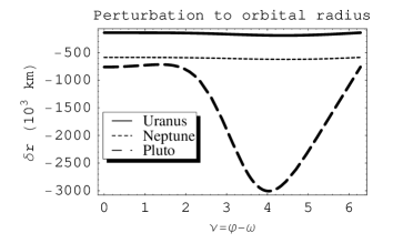
Figure 1: Gross perturbation to orbital radius $({10}^{3}\mathrm{km})$ over a complete period for the three outer planets

The perturbation $\delta\dot{\varphi}$ to the angular velocity is given by eq. 13, and the $e^{0}$ perturbation is $\delta{\dot{\varphi}}^{(0)}=2\kappa\dot{\varphi}$. Evaluating it for the three outer planets gives values of $1.7,2.1$ and $2.4$ arc sec/year for Uranus, Neptune and Pluto, respectively. $\dot{\varphi}(\nu)$ is plotted in Figure 2. The variation in the perturbation $\delta\dot{\varphi}$ over the orbital period is shown in Figure 2. As we can see, Pluto has the strongest variation in angular velocity, which is because of the proportionality $\delta\dot{\varphi}\propto-\delta r/r^{3}$. $\delta\dot{\varphi}$ increases as $\sqrt{a}$ with orbital radius, and we can clearly see from Figure 2 that there is stronger variation in the angular velocity perturbation for orbits with higher eccentricity.

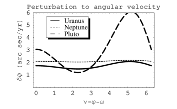
Figure 2: Gross perturbation to angular velocity in arc sec/year over a complete period for the three outer planets

The perturbation to the argument of latitude, $\delta\varphi$,  is given by eq. 14. The $e^{0}$ term of the perturbation to the angular velocity $\delta\dot{\varphi}$ implies a large secular increase of $\delta\varphi$, which is apparent in the plot of $\delta\varphi$ in Figure 3. For Uranus and Neptune, the secular effect is completely dominant, and $\delta\varphi$ increases almost linearly with $\varphi$. For Pluto, however, the big variation in $\delta\dot{\varphi}$ that can be seen in Figure 2 makes $\delta\varphi$ for Pluto deviate significantly from a linear increase.

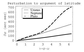
Figure 3: Gross perturbation to the argument of latitude $\varphi$ (arc sec) over a complete period for the three outer planets

If these perturbations were real, one would expect that by fitting a Keplerian orbit to them that has a slightly higher mean motion, one would be able to cancel the secular increase. This can easily be seen by the following example: If the mean motion was increased by an amount equal to the secular term $\delta{\dot{\varphi}}^{(0)}=2\kappa\dot{\varphi}$, we would expect the resulting residuals to show no secular increase. Figure 4 shows the net perturbation $\delta\varphi-{\delta\varphi}^{(0)}$ for Uranus and Neptune after removing the secular term ${\delta\varphi}^{(0)}$. As would be expected, the net perturbations are much smaller, of the order of a few arc seconds. Notice that, although the gross $\delta\varphi$ perturbation of Neptune grew much faster than $\delta\varphi$ for Uranus, due to its higher $\kappa$, the net perturbations for Neptune is considerably smaller, due to its low eccentricity.

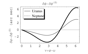
Figure 4: The net perturbation to the argument of latitude after removal of the zero-order secular term

Later, in Section V, we will make a thorough best fit of these $\delta$$\varphi$ perturbations to Keplerian orbits in order to find the minimal net perturbations for the three outer planets.

III Perturbations to planetary orbits - General Metric Theory of Gravitation

Now, let us generalize the calculation of the preceeding section and just assume that the gravitational field can be described by a metric theory of gravitation. This is a very general case that includes any PPN-parametrizable theory, including General Relativity. The purpose of this generalization is to include cases where the hypothetical perturbation to the gravitational field is not due to the presence of a gravitational source, but rather is caused by a deviation in the long-range behavior of the gravitational field from the behavior expected from General Relativity. As mentioned in section I, alternative gravitational theories have been proposed as explanations for the Pioneer anomaly, so we would like our analysis to be able to cover such cases.

III.1 Deriving the disturbance to the gravitational field

Our first task is to analyze what constraints the introduction of a constant anomalous radial acceleration would put on the metric of the surrounding space. We assume a spherically symmetric metric, and begin by studying the dynamics of a body moving geodesically in a static, spherically symmetric, helio-centric gravitational field that can be described by a metric of the form

$${\mathrm{ds}}^{2}=-B(r)c^{2}{\mathrm{dt}}^{2}+{A(r)}^{-1}{\mathrm{dr}}^{2}+r^{2}({\mathrm{d\theta}}^{2}+{\sin}^{2}\theta{\mathrm{d\varphi}}^{2})$$ (15)

An object with rest-mass $\mu>0$ moving geodesically in this gravitational field has two constants of motion; the total energy, $E$, and the angular momentum, $L$:

$$E=\mu{c}^{2}B\frac{\mathrm{dt}}{\mathrm{d\tau}},L=\mu r^{2}\frac{\mathrm{d\varphi}}{\mathrm{d\tau}},$$ (16)

where $\tau$ is the proper time of the moving body. The motion is planar, and we have chosen coordinates so that the plane of motion coincides with the plane given by $\theta=\pi/2$. Writing the invariant $g_{\mu\nu}p^{\mu}p^{\nu}=-\mu^{2}c^{2}$ in the coordinates of eq. 15 and applying the constants of motion of eq. 16  yields the following equations describing geodesic motion in a static, spherically symmetric gravitational field Misner-Thorne-Wheeler-1973 :

$$\frac{1}{c^{2}}{\left(\frac{dr}{d\tau}\right)}^{2}=\mathcal{E}^{2}\frac{A}{B}-A(1+\frac{\ell^{2}}{c^{2}r^{2}})$$ (17)

$$\frac{d\varphi}{d\tau}=\frac{\ell}{r^{2}}$$ (18)

$$\frac{dt}{d\tau}=\frac{\mathcal{E}}{B}.$$ (19)

Here we have introduced the constants $\mathcal{E}\equiv E/\mu c^{2}$ (total energy per unit rest energy) and $\ell\equiv L/\mu$ (total angular momentum per unit rest mass). Notice that for bodies moving non-relativistically at speed $v$,  $\mathcal{E}=\sqrt{B(1+{(v/c)}^{2})}\simeq 1+\frac{1}{2}{(\frac{v}{c})}^{2}-\frac{GM}{c^{2}r}$, which is very close to unity. For the three outer planets,  $1-\mathcal{E}=\mathcal{O}({10}^{-10})$.

Notice that these equations are valid for any metric theory of gravitation, and that we are not making any further assumptions on the  gravitational interaction besides minimal gravitational coupling, i.e. a body moving freely in a gravitational field moves geodesically.

In Newtonian gravity, a constant radial acceleration corresponds to an additional term in the gravitational potential that is linear in $r$. We then write the metric functions $A$ and $B$ as sums of the metric function $B_{0}=1-2GM/c^{2}r$ of General Relativity (representing the unperturbed, expected value of the gravitational field) and a small perturbation, representing the metric disturbance necessary to generate the Pioneer anomaly:

$$A(r)\equiv B_{0}(r)+\alpha(r),B(r)\equiv B_{0}(r)+\beta(r).$$ (20)

The metric ${\mathrm{ds}}_{0}^{2}=-B_{0}c^{2}{\mathrm{dt}}^{2}+B_{0}^{-1}{\mathrm{dr}}^{2}+r^{2}{\mathrm{d\Omega}}^{2}$ corresponds to a spherically symmetric vacuum gravitational field around a central body with mass $M$. We assume $\alpha$ and $\beta$ both to be much smaller than $B_{0}$, which allows us to expand perturbatively around well-known solutions for the spherically symmetric vacuum field case. We will refer to the metric ${\mathrm{ds}}_{0}^{2}$ as the unperturbed metric. Expressing the radial equation, eq. 17, to first order in $\alpha$ and $\beta$, we get

$$\frac{1}{c^{2}}{\left(\frac{\mathrm{dr}}{\mathrm{d\tau}}\right)}^{2}=\left(\mathcal{E}^{2}+\left(\frac{\mathcal{E}^{2}}{B_{0}}-1\right)\alpha-\frac{\mathcal{E}^{2}}{B_{0}}\beta\right)\\ -B_{0}(1+\frac{\ell^{2}}{c^{2}r^{2}})$$ (21)

In the following, we restrict our analysis to non-relativistic motion and weak gravitational fields. In this regime, the $\alpha$-dependence of eq. 21 can be discarded, because, with $v$ being the velocity of the moving object,  $\frac{\mathcal{E}^{2}}{B_{0}}-1={(\frac{v}{c})}^{2}<<1$. Differentiating eq. 21 with respect to proper time $\tau$, we get the expression for the radial acceleration:

$$\frac{d^{2}r}{{\mathrm{d\tau}}^{2}}=-\frac{1}{2}{c^{2}(B_{0}(1+\frac{\ell^{2}}{c^{2}r^{2}}))}^{\prime}-\frac{1}{2}{c}^{2}\beta^{\prime},$$

where prime denotes differentiation wrt. the radial coordinate $r$. The first term on the right-hand side of this equation is the expected radial acceleration generated by the unperturbed vacuum metric. The last term on the right-hand side can be seen as an anomalous acceleration produced by an anomalous term $\beta$ in the $g_{00}$ component of the metric. In order for $-\frac{1}{2}{c}^{2}\beta^{\prime}$ to be a constant, negative acceleration, $\beta$ must be linear in r:

$$\beta=Pr,$$ (22)

with $P$ being a positive constant of dimension $1/r$. It should be noted that in order to compute the anomalous acceleration observed by a distant observer, we should transform eq. 21 to the proper reference frame of the observer, which for a distant observer would correspond to coordinate time t at the location of the observer. However, as $|\mathrm{dt}/\mathrm{d\tau}-1|=\mathcal{O}({10}^{-9})$for the velocities and astronomical distances we are considering, we can safely equate proper time $\tau$ with coordinate time $t$. If $a_{P}$ is the anomalous acceleration, directed towards the Sun, eq. 22 immediately gives us the relationship between the metric parameter  $P$ and $a_{P}$: $P=2a_{P}/c^{2}\mathcal{E}^{2}$.

We can conclude that an observed constant anomalous acceleration uniquely constrains the dominant part of the disturbance to the gravitational potential. An additional term, linear in $r$, must be present in the $g_{00}$ component of the metric in order to produce such an effect. This result is the same we get from Newtonian gravity. The analysis is independent of how this metric disturbance is produced, and is therefore also independent of the particular gravitational theory applied to analyze the the disturbance.

III.2 Equations of motion

Having found the perturbation to the gravitational field, we are now ready to explore the equations of motion for a body moving geodesically in this field. When discarding the $\alpha$-term of eq. 21 and using that $\frac{\mathcal{E}^{2}}{B_{0}}\beta\simeq\beta$, we  get the radial equation of motion

$$\frac{1}{c^{2}}{\left(\frac{\mathrm{dr}}{\mathrm{d\tau}}\right)}^{2}=\left(\mathcal{E}^{2}-\beta\right)-B_{0}(1+\frac{\ell^{2}}{c^{2}r^{2}})$$ (23)

By using eq. 18,  expressing the equation in terms of the reciprocal radial coordinate $u\equiv 1/r$,  taking the derivative of the equation with respect to $\varphi$ and using eq. 22, we get the following  second-order equation for $u(\varphi)$:

$$\frac{d^{2}u}{{\mathrm{d\varphi}}^{2}}+\left(1-\frac{3GM}{c^{2}}u\right)u=\frac{GM}{\ell^{2}}+\frac{a_{P}}{\ell^{2}\mathcal{E}^{2}}\frac{1}{u^{2}}$$ (24)

The unperturbed $(a_{p}=0)\text{}$ equation has the following approximate solution valid for low eccentricity orbits Misner-Thorne-Wheeler-1973 ; Carroll-2004 :

$$\frac{1}{u_{0}}=r_{0}=\frac{a(1-e^{2})}{1+e\cos\left(f\left(\varphi-\omega_{0}\right)\right)},$$ (25)

where $e$ is the eccentricity of the orbit, $\omega_{0}$ is the argument of the perihelion at a time when the planet is at perihelion, and $f^{2}=1-6{(\frac{GM}{c\ell})}^{2}\rightarrow 1$ as $r_{0}\rightarrow\infty$. $f$ is very close to unity. When setting $f=1$ we get the closed Keplerian orbits of eq. 4. In general, a factor $f<1$ yields a small relativistic perihelion precession, which for low eccentricity orbits is $\simeq 6\pi GM/(c^{2}a(1-e^{2}))$  per cycle. Evaluating the relativistic perihelion precession for the three outer planets gives values of of the order of ${10}^{-3}$ arc second per cycle. This is well below what would be observable, given the present data and their accuracy, which is of the order of 0.5 arc second.

Let us proceed as we did for for the Newtonian case of Section II.2  and assume that $u_{0}$ is a reference solution to the unperturbed equations of motion, of the form given by eq. 25. Let us then define the perturbation $\delta u=u-u_{0}$, where $u$ is a solution to the perturbed equation of motion, eq. 24, having the same angular momentum $\ell$ as $u_{0}$. We obtain the following equation of motion for the perturbation $\delta u$:

$$\frac{d^{2}\delta u}{{\mathrm{d\varphi}}^{2}}+\left(f^{2}+2\kappa\right)\delta u=\frac{\kappa}{a(1-e^{2}){\left(1+e\cos\left(f\nu\right)\right)}^{2}},$$ (26)

where $\nu\equiv\varphi-\omega_{0},\kappa\equiv\frac{a_{p}}{a_{N}}{(1-e^{2})}^{2},a_{N}\equiv\frac{GM}{a^{2}}$, as in the Newtonian case before. Now, $1-f^{2}$ is of the order ${10}^{-9}$ for the three outer planets. Since $\kappa$ is $\mathcal{O}({10}^{-4})$, we can safely ignore any Post-Newtonian corrections to the solutions, set $f=1$ and proceed with the Newtonian equation of motion, eq. 7 and the corresponding solutions, as derived in section II.

IV Analysis Method

IV.1 Observations and their residuals

The procedures that are applied for calculating the ephemerides of the planets use available theory, taking into account known gravitational sources, and carefully fitting the computations to available observational data Standish-1998 ; Pitjeva-2005a . One would therefore expect that any disturbance to the gravitational field within the solar system would, if large enough, over time generate residuals in the position measurements of the planets as they would tend to drift from their expected positions. The question then is, what residuals would arise if we were to explain the Pioneer anomaly as the result of a perturbation to the gravitational field in the outer solar system, and how do they compare with the observed residuals? In this section, we will elaborate the analysis method which we will apply in order to answer these questions.

Before we start our analysis, let us review what the observables are and how to compare models with observations. See Appendix B for a review of terminology and notation used. When restricted to performing optical observations only of a distant object, which has been the case for the three outer planets, there are just two observables: the right ascension (r.a.),  and declination (dec.). These are the position angles that locate the object on the celestial sphere. Accurate optical measurements of the positions of the outer planets have been performed since the early 20th century. The a priori uncertainty of these measurements were $0.5-1$ arc second during most of this period Pitjeva-2005a . In recent years, the a priori accuracy has been improved to $~{}0.2$ arc second. Computational models of the motion of the known objects in the Solar System can then be applied to compute the ephemerides, which are the expected orbits, of these objects. The free parameters of the model are fixed by making a best fit of the computations with the observations. The results are the Solar System Ephemerides, composed of highly accurate maps of the motions of the planets as well as other known Solar System bodies Pitjeva-2005a ; Standish-1998 .

Figure 5: Actual r.a. residuals (in arc seconds) for the three outer planets, courtesy of E.M. Standish, JPL

Figure 5 shows the DE414 residualsStandish-1998 in right ascension for the three outer planets. These residuals are the difference between the measured and ephemeris right ascension values, taken over the entire span of available data. As could be expected, the residuals are smaller towards the end of the data span, apparently due to the increased accuracy of the measurement techniques applied. Table 1 gives the standard deviations of the r.a. residuals for the three outer planets. The standard deviations of these residuals are within the a priori measurement accuracies that have been reported Standish-1998 ; Pitjeva-2005a .

Table 1: Standard deviations in right ascension residuals for the three outer planets

Planet	Std. dev - $\sigma_{l}$ (arc sec.)
Uranus	0.3
Neptune	0.3
Pluto	0.8

IV.2 Description of the analysis method

Our best option for determining whether or not a perturbation to the gravitational field would have an observable effect on the motions of the outer planets is to solve the basic equations of motion for the three planets under the hypothesis of a perturbed gravitational field. The purpose of these solutions,  referred to as the simulated observations orbits, is to provide targets for best fit approximations using solutions to the unperturbed equations of motion. Just like real ephemerides emerge as best fits of solutions of the equations of motion to the real observations, we will construct simulated ephemerides by fitting solutions of the unperturbed equations of motion  to the simulated observations orbits. The simulated ephemerides obtained this way therefore play the same role as the real ephemerides, i.e. the best fit of known models to observations. From the simulated observations orbit and the corresponding simulated ephemeris, we can derive the corresponding values of the optical observables; the right ascension $\alpha$ and the declination $\delta$ and their residuals. These residuals (simulated obs. value - simulated ephemeris value), which are derived from the basic equations of motion, provide a realistic lowest order estimate of the residuals in the observables to be expected from a perturbation to the gravitatational field of the kind required to account for the Pioneer anomaly.

Although we work with models that are idealized compared to the realistic models underlying modern planetary ephemerides, we still expect the simulated residual estimates to be realistic to lowest order in the perturbations, because to lowest order, perturbations decouple and can be studied independently.

Finally, since we would like to compare the results of the hypothetical model to real observations, we will define the predicted observations to be the sum of the real ephemeris values and the best fit simulated residuals. The underlying assumption here is that the simulated residuals can be used to predict the offset between the ephemeris and the expected observations under the hypothesis of a perturbed gravitational field. This is the closest we can get with respect to checking this hypothesis against data. We are not interested in the predicted observations themselves, only in their residual relative to the real observations. As we will see later, the (real -predicted) residual can be estimated by combining the real and simulated residuals.

Having obtained the simulated residuals as the difference between the simulated observations and the simulated ephemerides, the remaining problem is how to compare them with the real residuals, described in section IV.1 above. Let us formulate two hypotheses that we would like to test by statistical methods:

H1: Given the uncertainty of the observations, the simulated r.a. observations do not deviate significantly from the simulated ephemerides

H2: Given the uncertainty of the observations, the predicted r.a. observations do not deviate significantly from the real observations

Hypothesis H1 is testing, under the assumption of a perturbed gravitational field, whether the ephemerides still would provide good fits to the observations. If not, it would contradict the present state of matters, because the ephmerides do provide good fits to the data.

Hypothesis H2 tests, again under the assumption of a perturbed gravitational field, whether the model predictions are consistent with the actual observations.

Now, let us restate the original hypothesis stated in Section I.2 above:

H0: The Pioneers move geodesically in a perturbed gravitational field

The logical connection between hypothesis H0 and the other two should be clear. H0 is falsified if any of hypotheses H1 and H2 are falsified, because falsification of H1 or H2 would imply that a perturbation to the gravitational field required to induce the Pioneer anomaly is not present. On the other hand, H1 and H2 can obviously not be used to verify H0.

Notice that the results will critically depend on judicial estimates of the measurement uncertainties. For a given planet $l$, we will use the standard deviation $\sigma_{l}$ of the r.a. residuals shown in Figure 5 as the best estimate of the uncertainty in the observations. If the ephemeris provides a good match to the observations, it is reasonable to assume that $\sigma_{l}$ will be close to the measurement uncertainty. If not, $\sigma_{l}$ would be  higher than the measurement uncertainty. In either case, using $\sigma_{l}$ as a best estimate of the uncertainty in the measurements seems a reasonable, if not conservative, choice.

In order to test hypotheses H1 and H2, we will perform a chi square analysis with a confidence limit of 99%. Let us elaborate how we will apply this method in our case. Given $N_{l}$ measurements $({\hat{\alpha}}_{l,j},t_{j})$ of the right ascension for planet $l$ at measurement times $t_{j}$, the real residuals $\rho_{l,j}(t_{j})$ for planet $l$ is the difference between the observation ${\hat{\alpha}}_{l,j}$ and the corresponding ephemeris value  $\alpha_{l}(t_{j})$:  $\rho_{l,j}(t_{j})\equiv{\hat{\alpha}}_{l,j}-\alpha_{l}(t_{j})$. These are the residuals that are plotted in Figure 5 above, which we will refer to as the real residuals.

Given a solution to the equations of motion for planet $l$ under the hypothesis that the gravitational field is perturbed by a constant radial acceleration $a_{p}$ directed towards the Sun, we can derive the set of simulated right ascension values ${\hat{\alpha}}_{l}^{P}(t_{j})$. We will refer to these as our set of simulated observations. The simulated ephemeris is the solution of the unperturbed equations of motion that provides the best fit to the simulated observations orbits, and from it we can derive a set of simulated right ascension ephemeris values $\alpha_{l}^{P}(t_{j})$. The simulated residuals $\rho_{l,j}^{P}$ are then the difference between the simulated right ascension values and the corresponding simulated ephemeris values: $\rho_{l,j}^{P}(t_{j})\equiv{\hat{\alpha}}_{l,j}^{P}(t_{j})-\alpha_{l}^{P}(t_{j})$.

The predicted r.a. value ${\hat{\alpha}}_{l,j}^{P^{\prime}}(t_{j})$ is the sum of the real ephemeris value $\alpha_{l}(t_{j})$ and the simulated residual $\rho_{l,j}^{P}$:

$${\hat{\alpha}}_{l,j}^{P^{\prime}}(t_{j})\equiv\alpha_{l}(t_{j})+\rho_{l,j}^{P}$$ (27)

Define the real-predicted observation residual  $\rho_{l,j}^{P^{\prime}}$ to be the difference between the real observation and the predicted observation:

$$\rho_{l,j}^{P^{\prime}}\equiv{\hat{\alpha}}_{l,j}\left(t_{j}\right)-{\hat{\alpha}}_{l,j}^{P^{\prime}}(t_{j})=\rho_{l,j}(t_{j})-\rho_{l,j}^{P}(t_{j})$$ (28)

We see from eq. 28 that we can estimate the real-predicted observation residuals by combining the real residuals $\rho_{l,j}(t_{j})$ with the simulated residuals $\rho_{l,j}^{P}(t_{j})$. This allows us to compare the predicted observations with the real observations using the chi square method.

Let $\sigma_{l}^{2}$ be the variance of the real residuals for planet $l$. As discussed previously, we will assume that $\sigma_{l}$ is a good estimate of the measurement uncertainty. Now, define the following chi square values that we will use to test the hypotheses above:

$$\chi_{l,1}^{2}\equiv\frac{1}{\sigma_{l}^{2}}\sum\limits_{j=1}^{N_{l}}\rho_{l,j}^{P}{\left(t_{j}\right)}^{2}$$ (29)

$$\chi_{l,2}^{2}\equiv\frac{1}{\sigma_{l}^{2}}\sum\limits_{j=1}^{N_{l}}{\left(\rho_{l,j}^{P^{\prime}}\right)}^{2}$$ (30)

Provided measurement errors are distributed normally, a model deviates from observations with probability $p$ if the $\chi^{2}$ of the residuals between the observations and the model prediction exceeds $N_{l}+C_{p}$, where $C_{p}$ is the confidence limit applied. $C_{p}$ depends on the probability given (the confidence level) and the number of free parameters. In our case, the number of free parameters is 4, and we have chosen a confidence level of 0.99. This gives $C_{p}=13$.

$\chi_{l,1}^{2}$ can be used to test hypothesis H1 above; if $\chi_{l,1}^{2}>N_{l}+C_{p}$, the deviation of the simulated r.a. observations from the simulated ephemeris is statistically significant at a significance level of $p$. Similarly,  $\chi_{l,2}^{2}$ can be used to test hypothesis H2 above; if $\chi_{l,2}^{2}>N_{l}+C_{p}$, the deviation of the projected r.a. observations from the real observations is statistically significant at a significance level of $p$.

IV.3 Comments on the perturbative approach for solving the equations of motion

In this paper, we study what observational effects a disturbance to the gravitational field would have on orbits of a planet moving in a static, spherically symmetric gravitational field around the Sun. We work perturbatively to lowest order in the perturbation. Since we are looking for dominant effects only, we are free to disregard other perturbing effects, such as the presence of other bodies in the Solar System. These simplifications allow us to treat the problem analytically.

In section II, we started our analysis by choosing a reference orbit, which is an idealized orbit satisfying the unperturbed equations of motion and matching the orbital parameters of one of the three outer planets. In the Newtonian case, the reference orbit is a Keplerian orbit that is set up by applying the mean Keplerian elements of the planet as initial conditions. This reference orbit has no other role than being the reference for two perturbations:

In section II, we found the first pertubation, which gives rise to the simulated observations. It comes from solving the equations of motion for a perturbed gravitational field. For this orbit, the simulated observations orbit, we applied the assumption that the gravitational field is perturbed in a way that results in a constant, anomalous radial acceleration $a_{P}\equiv 8.7\times{10}^{-10}m/s$ towards the Sun. By integrating the equations of motion, we obtained the perturbation to the argument of latitude, denoted by $\delta\varphi$. The argument of latitude, $\varphi$, is related to the true anomaly, $\nu$, by $\varphi\equiv\omega+\nu$, where $\omega$ is the argument of periapsis . In our case, $\omega$ is the argument of periapsis of the reference orbit, i.e. a fixed position. If $\varphi_{0}(t)$ is the argument of latitude of the reference orbit, $\varphi_{p}(t)=\varphi_{0}(t)+\delta\varphi(t)$ is the argument of latitude of the perturbed orbit. Thus, we can derive expected values for the $\alpha$ and $\delta$ observables from $\varphi_{p}$ by performing a coordinate transformation of the position  vector $(r_{p},\varphi_{p})$ in the orbital plane of the planet to geocentric equatorial coordinates.

The second perturbation, which we will refer to as our simulated ephemeris,  arises when we attempt to find the solution that best fits the simulated observations orbit $(r_{p},\varphi_{p})$. In order to simplify the analytical treatment, we assume that this solution can be treated as a perturbation, denoted $\Delta\varphi$, to the reference orbit as well. Having found the best fit solution by performing a least squares approximation of the second perturbed orbit $(r_{E}(t)=r_{0}(t)+\Delta r(t),\varphi_{E}(t)=\varphi_{0}(t)+\Delta\varphi(t))$ to the simulated observations orbit $(r_{p},\varphi_{p})$, we can estimate the simulated residuals in $\alpha$ and $\delta$ as the difference between the values of the simulated observations and the simulated ephemeris, as described in section IV.2.

V Residual Analysis

If $(r_{0}(\varphi_{0}),\varphi_{0}(t))$ is the reference orbit, $(r_{p}(\varphi)=r_{0}(\varphi_{0})+\delta r(\varphi_{0}),\varphi_{p}(t)=\varphi_{0}(t)+\delta\varphi(\varphi_{0}))$ is the simulated observations orbit, i.e. the perturbed orbit from which we can derive simulated observations. The simulated observations orbit was derived in section II. Now it is time to proceed with the next step of our analysis: Following the analysis procedure outlined in Section IV.2 above, our next task is to compute the simulated ephemeris, which is the  Keplerian orbit that provides the best fit to the simulated observations orbit.

V.1 Finding the simulated ephemerides

Eq. 3 represents the unperturbed equation of motion that we will solve. Since the simulated observations orbit $(r_{p}(\varphi),\varphi_{p}(t))$ is just a perturbation of the reference orbit $(r_{0},\varphi_{0})$, we can assume that the best fit Keplerian orbit, our simulated ephemeris, also represents a pertubation to the reference orbit. Perturbing eq. 3 gives the equation for the radial perturbation $\Delta u\equiv u-u_{0}$, where $u$  here is another Keplerian orbit with angular momentum $\ell\equiv\ell_{0}+\Delta\ell$:

$$\frac{d^{2}\Delta u}{{\mathrm{d\varphi}}^{2}}+\Delta u=-\frac{2}{a(1-e^{2})}\frac{\Delta\ell}{\ell_{0}}.$$ (31)

Eq. 31 has the general solution

$$\Delta u=\frac{1}{a}\left(eC_{1}\sin\ \ \nu+eC_{2}\cos\nu-\frac{2}{\left(1-e^{2}\right)}\frac{\Delta\ell}{\ell_{0}}\right),$$ (32)

where $C_{1}$, $C_{2}$ and $\Delta$$\ell$ will be treated as free parameters. Similarly to how we derived eq. 11, we get the equation for the angular perturbation:

$$\frac{d\Delta\varphi}{\mathrm{d\varphi}}=\frac{\Delta\ell}{\ell_{0}}-2\frac{\Delta r}{r_{0}}$$ (33)

The exact solution to eq. 33 is

$$\Delta\varphi=C_{0}+\left(\frac{\Delta\ell}{\ell}+2C_{2}\left(1-e^{2}\right)\right)\nu-2C_{1}(1-e^{2})\ln(1+e\cos\nu)-\frac{4}{\sqrt{1-e^{2}}}\left(2\frac{\Delta\ell}{\ell}+C_{2}(1-e^{2})\right)\arctan(\sqrt{\frac{1-e}{1+e}}\tan\frac{\nu}{2})$$ (34)

Define $u_{K}\equiv u_{0}+\Delta u$ and  $\varphi_{K}\equiv\varphi_{0}+\Delta\varphi$. $\Delta\varphi$ introduces another free parameter $C_{0}$. This leaves us with four free parameters that we will fit to the simulated orbit: $C_{0}$, $C_{1}$, $C_{2}$ and $\Delta$$\ell$.

Define the simulated residual $\hat{\Delta\varphi}$ by  $\hat{\Delta\varphi}\equiv\varphi_{p}(\varphi_{0})-\varphi_{K}(\varphi_{0})=\delta\varphi-\Delta\varphi$. The simulated residual $\hat{\Delta\varphi}$  can be written in the form

$$\hat{\Delta\varphi}=\delta\varphi-C_{0}+\frac{\Delta\ell}{\ell}f_{0}(\varphi)+C_{1}f_{1}(\varphi)+C_{2}f_{2}(\varphi),$$ (35)

where $f_{0},f_{1}$ and $f_{2}$ are functions that to third order in eccentricity take the form

$$f_{0}\equiv\left(3+2e^{2}\right)\nu-e\left(4+3e^{2}\right)\sin\nu+e^{2}\sin 2\nu\\ -\frac{e^{3}}{3}\sin 3\nu+\mathcal{O}(e^{4})$$

$$f_{1}\equiv e\left\{-\frac{e}{2}\ \ +\left(2-\frac{3}{2}e^{2}\right)\cos\nu-\frac{e}{2}\cos 2\nu+\frac{e^{2}}{6}\cos 3\nu\right\}\\ +\mathcal{O}(e^{4})$$

$$f_{2}\equiv e\left\{e\nu-\left(2-\frac{e^{2}}{2}\right)\sin\nu+\frac{e}{2}\sin 2\nu-\frac{e^{2}}{6}\sin 3\nu\right\}\\ +\mathcal{O}(e^{4})$$

Let us consider for a moment the circular limits of eqs. 32 and 35.  In that case, $f_{1}=f_{2}=0$. Eqs. 9 and 32 show that in the circular limit, the simulated radial residual $\delta u-\Delta u$ can be eliminated by properly adjusting the angular momentum of the the Keplerian orbit. However, in this case we are left with a non-vanishing simulated angular residual $\hat{\Delta\varphi}$. If we, on the other hand, adjust the angular momentum and $C_{0}$ to make the angular residual $\hat{\Delta\varphi}$ vanish, we are left with a non-zero radial residual $\hat{\Delta r}\equiv\delta r-\Delta r=\kappa a/3$. Thus, even in the circular limit, we can not simultaneously fit both the angular and radial perturbations by a Keplerian orbit. When projecting $\hat{\Delta r}$ onto the celestial sphere for the near circular orbits of Uranus and Neptune, it translates to perturbations in the observation angles of $0.2"$ and $0.3"$, respectively. This implies that in the circular limit, even if the angular residual $\hat{\Delta\varphi}$ can be eliminated by adjusting the angular momentum, the Pioneer effect is in principle still observable from the perturbation to the observation angle resulting from the non-vanishing radial residual $\hat{\Delta r}$. In the following, we will make a best fit of the simulated angular residual $\hat{\Delta\varphi}$ and ignore the effect of the remaining radial perturbation on the observable angle.

Now, let us define the best fit solution $(r_{E},\varphi_{E})$ as the solution $(r_{K},\varphi_{K})$ that minimizes the variance of the simulated residual $\hat{\Delta\varphi}$ over the measurement interval [$t_{0},t_{1}$]:

$$\sigma_{p}^{2}\equiv\frac{1}{\left(\varphi(t_{1})-\varphi(t_{0})\right)}\operatorname*{\overset{\varphi(t_{1})}{\int}}\limits_{\varphi(t_{0})}d\varphi\ \ {\hat{\Delta\varphi}}^{2}$$ (36)

The best fit is made by finding the values of the free parameters $\Delta\ell$, $C_{0}$, $C_{1}$ and $C_{2}$ that give minimal variance $\sigma_{p}^{2}$. Equation 36 can be integrated analytically, and gives a second order polynomial in the free parameters $C_{0}$, $C_{1}$, $C_{2}$ and $\Delta$$\ell$. This polynomial has a unique minimum that can be found by solving the equations $\frac{\partial}{\partial C_{0}}\sigma_{p}^{2}=0$ , $\frac{\partial}{\partial C_{1}}\sigma_{p}^{2}=0$, $\frac{\partial}{\partial C_{2}}\sigma_{p}^{2}=0$ and $\frac{\partial}{\partial\Delta\ell}\sigma_{p}^{2}=0$.

V.2 Analyzing the simulated residuals

Figure 6 plots $-\rho^{p^{\prime}}$, the predicted-real r.a. residuals, and the simulated r.a. residuals for the three outer planets. In order to make the simulated residuals easy to compare with the real residuals, a coordinate transformation of the orbit to the mean equatorial plane has been done. The plots also show the standard deviations of the real residuals.

Figure 6: Simulated (solid lines) and predicted-real r.a. residuals (in arc seconds) for the three outer planets. Dashed lines indicate the standard deviation of the real residuals.

From Figure 6 we can immediately see that the simulated residuals for Neptune are very small compared to the real residuals. This implies that a Pioneer-type perturbation would have no observable effect on the orbit of Neptune. Furthermore, by visual inspection of the real-predicted residuals in  Figure 6, we see that there are significant deviations between real and predicted observations for Uranus and Pluto.

Now, let us put this on formal grounds and test hypotheses H1 and H2 formulated in Section IV.2 above. Given the simulated residuals $\rho^{p}$ and the real residuals $\rho$, we must compute the chi square values $\chi_{l,1}^{2}$  and $\chi_{l,2}^{2}$ that target these hypotheses. Table 2 shows the results of this computation and the tests of hypotheses H1 and H2 for each of the three outer planets.

Table 2: Chi square values of the simulated residuals for the three outer planets and the results of the tests of hypotheses H1 and H2 of Section IV.2

Planet	$\sigma_{l}(")$	$N_{l}$	$\chi_{l,1}^{2}-N_{l}$	$\chi_{l,2}^{2}-N_{l}$	H1	H2
Uranus	0.283	3678	486	4930	False	False
Neptune	0.293	3800	-3799	6.5	True	True
Pluto	0.771	2119	-1510	773	True	False

The main conclusions drawn from this analysis are that, given an uncertainty $\sigma_{l}$ in the r.a. observations:

1. For Uranus, the simulated r.a. observations show a deviation from the simulated ephemeris that is statististically significant well beyond the 99% confidence level. For Pluto, however, no such deviation is found for the simulated r.a. observations. Thus, H1 is falsified for Uranus and verified for the other two planets.

2. For both Uranus and Pluto, the predicted r.a. observations show a deviation from the real r.a. observations that is statististically significant well beyond the 99% confidence level. Thus, H2 is falsified for Uranus and Pluto, but verified for Neptune.

VI Conclusions

Under the assumption that the observed frequency drift of the Pioneer spacecraft is caused by a constant, anomalous acceleration that is directed towards the Sun, and that the Pioneer spacecraft move geodesically in a perturbed gravitational field that is static and spherically symmetric, we have analyzed the effects that such a perturbation to the gravitational field would have on the orbits of the three outer planets. The basic assumptions are that the gravitational field can be modeled within a metric theory of gravity and that particles couple minimally to the gravitational field, i.e. they move geodesically when falling freely in a gravitational field. Our results are model independent within this class of theories in the sense that they do not depend on the particulars of the gravitational theory, e.g. the nature of any gravitational source or how gravitational sources couple to the spacetime metric. The analysis is valid in the weak field limit of any metric gravitational theory, and it therefore applies to any gravitational theory that can be parametrized within the PPN framework.

We showed in section III.1 that the metric perturbation that would be needed to induce the Pioneer anomaly can be uniquely constrained to lowest order. This immediately implies that perturbed orbits due to the perturbation in the gravitational field will be the same, to lowest order in the perturbation, for all metric theories of gravity. Furthermore, by solving the basic equations of motion for a perturbed gravitational field, we indeed found that Post-Newtonian effects were small compared to Newtonian effects.

By solving the unperturbed equations of motion and finding the solutions that provide the best fit to the perturbed solutions, we were able to derive simulated right ascension residuals that could be compared with the real ephemeris residuals.

We then formulated an analysis method, based on the chi square method, for comparing simulated residuals with the real ephemeris residuals. We formulated two hypotheses that, if falsified, would falsify the hypothesis of the presence of a perturbation to the gravitational field. Following from Einstein’s equivalence principle, this would imply that the Pioneers do not move geodesically in a perturbed gravitational field. Hypothesis H1 tests, under the assumption of a perturbed gravitational field, whether the ephemeris still provides a good fit to the observations expected from a perturbation to the gravitational field. If not, it would contradict the present state of matters, because the ephemerides do provide good fits to the data. Hypothesis H2 tests, again under the assumption of a perturbed gravitational field, whether the model predictions emerging from the model of a perturbed gravitational field are consistent with the actual observations. Falsification of either H1 or H2 would imply that a perturbation to the gravitational field required to induce the Pioneer anomaly is not present, which under Einstein’s equivalence principle would imply that the Pioneers do not move geodesically.

The analysis shows that the ephemerides provide good fits to the perturbed orbits expected from a perturbation to the gravitational field for Neptune and Pluto, but not for Uranus. Thus hypothesis H1 is falsified for Uranus. The fact that no significant deviation in the simulated residuals for Pluto is found can be attributed to the fact that the measurement uncertainty $\sigma_{l}$ for Pluto is higher than for the other two planets. Furthermore, the analysis also shows that the deviation between real and predicted r.a. observations is statistically significant for both Uranus and Pluto, implying that hypothesis H2 is falsified for both planets. The statistical significance of this result is well beyond the 99% confidence limit in both cases. For Neptune, on the other hand, we find no significant deviation, so hypothesis H2 is verified for Neptune. This is not surprising, because Neptune’s orbit has very low eccentricity, and, as we saw from the discussion of this subject in Section V.1, the angular residual arising from the Pioneer effect can be fitted out in the circular limit (the small perturbation to the observation angle that comes from projecting the remaining radial residual onto the celestial sphere is ignored in this study).

It should be stressed again that these conclusions rest on judicial esitmates of the uncertainties in the observations. We have chosen to use the standard deviations $\sigma_{l}$ of the real residuals as the best estimates of the measurement uncertainties.

Based on the available observations of the three outer planets, an assessment of their uncertainties and the available residuals between observations and ephemerides, we are therefore lead to the conclusion that the presence of a perturbation to the gravitational field necessary to induce the Pioneer anomaly is in conflict with available data. This implies that the Pioneer anomaly can not have gravitational origin and, consequently, the Pioneer spacecraft do not follow geodesic trajectories through space. Hence, any external interaction model introduced  to explain the Pioneer anomaly should, in one way or another, violate the equivalence principle. It should be stressed that “gravitational origin” in this context really means any physical interaction that is mediated indirectly via the space-time metric only. It is assumed here that particles move geodesically when moving under gravitational influence only (minimal coupling), so models implying other, non-minmal coupling schemes can not be excluded by our results. Our conclusion is consistent with recent findings of Iorio and Giudice Iorio-2006a as well as Izzo and Rathke Izzo-Rathke-2005 . It should be noted though, that while Iorio and Giudice find large secular effects on the orbits of the three outer planets, we find no such effects. The reason for this discrepancy is that, as shown here, any secular effects would be canceled by the simulated ephemeris, i.e. the best fit solution to the unperturbed equations of motion. The only observable effect is therefore the net residuals that still remain after the ephemeris cancels the big secular deviations.

This result can be used to rule out any model of the Pioneer anomaly that implies that the Pioneer spacecraft move geodesically through space and that explains the Pioneer anomaly as the effect of a disturbance to the spacetime metric, regardless of how this disturbance is created. This includes some of the proposed models of the anomaly mentioned in section I, such as scalar field modelsBertolami-Paramos-2005 , braneworld scenarios Bertolami-Paramos-2004 and models involving alternative metric theories of gravitation Jaekel-Reynaud-2005b ; Jaekel-Reynaud-2005 ; Bekenstein-2004 ; Bekenstein-Magueijo-2006 such as TeVeSBekenstein-2004 .

We conclude that, in order to resolve the enigma of the Pioneer anomaly, there is a need for theories and models that may explain the apparently non-geodesic motion of the Pioneer spacecraft.

Appendix A Pertubative expressions

Here, we provide the expansions to third order in eccentricity of the perturbative expressions given in Section II.2 above. All pertubative calculations were made with these third order expressions, so the results given in this paper are indeed valid to third order in eccentricity.

The $\mathcal{O}(e^{3})$ perturbation in reciprocal radial distance, $\delta u$, which to lowest order is given by  eq. 8, is

$$\delta u=\frac{\kappa}{a}\left(1+\frac{20}{8}e^{2}-\frac{e^{2}}{2}\cos 2\nu+\frac{e^{3}}{8}\cos 3\nu\right)\\ -\frac{e}{a}\left(1+\frac{5}{2}e^{2}\right)\cos\nu\\ +A\sin(\sqrt{1+2\kappa}\nu)+B\cos(\sqrt{1+2\kappa}\ \ \nu)+\mathcal{O}(e^{4})$$ (37)

Demanding $\delta u=0$ for $\kappa=0$ fixes $A$ and $B$ to take the values $A=0$ and $B=\frac{e}{a}(1+\frac{5}{2}e^{2})+\mathcal{O}(e^{4})$. This gives an angular perturbation

$$\delta u=\frac{\kappa}{a}\left\{1+\frac{20}{8}e^{2}-\frac{e^{2}}{2}\cos 2\nu+\frac{e^{3}}{8}\cos 3\nu\right.\\ \left.-e(1+\frac{5}{2}e^{2})\nu\sin\nu\right\}+\mathcal{O}(e^{4}).$$ (38)

The third order expression for the radial perturbation $\delta r$, corresponding to eq. 10, is

$$\delta r=-\kappa a\ \ \left\{1+2e^{2}-e\ \ \left(2+\frac{7}{2}e^{2}\right)\cos\nu+e^{2}\cos 2\nu\right.\\ -\frac{3}{8}e^{3}\cos 3\nu-e(1+\frac{5}{4}e^{2})\nu\sin\nu\\ \left.+e^{2}\nu\sin 2\nu-\frac{3}{4}e^{3}\nu\ \ \sin 3\nu\right\}+\mathcal{O}(e^{4}).$$ (39)

Expanding the equation for the angular perturbation to third order in eccentricity gives

$$\frac{d\delta\varphi}{d\varphi}=2\kappa\left\{1+2e^{2}-e(1+2e^{2})\cos\nu\right.\\ \left.-e\nu(1+2e^{2}-e\cos\nu+\frac{e^{2}}{2}\cos 2\nu)\sin\nu+\frac{1}{8}e^{3}\cos 3\nu\right\}\\ +\mathcal{O}(e^{4}).$$ (40)

Integration of eq. 40  wrt. $\varphi$ gives the angular perturbation corresponding to eq. 14:

$$\delta\varphi=\kappa\left\{\nu(2\left(1+2e^{2}\right)+\frac{e}{2}\left(4+7e^{2}\right)\ \ \cos\nu\right.\\ \left.-\frac{e^{2}}{6}\left(3\cos 2\nu-e\cos 3\nu\right)\right)\\ \left.-\frac{e}{2}\ \ \sin\nu\left(8+15e^{2}-e\cos\nu\right)+\frac{e^{3}}{36}\sin 3\nu\right\}+\mathcal{O}(e^{4}).$$ (41)

Appendix B Terminology and notation

Here, we provide a short review of the astonomical terminology and notation used in the paper. For a complete account of this terminology, see any astrodynamics textbook, such as Vallado-2001 .

The Ecliptic plane is the plane in which the Earth moves around the Sun. The Ecliptic is the cross section of the Ecliptic plane with the celestial sphere. The right ascension (r.a.) and declination (dec.) angles fix the object on the celestial sphere. These angles are measured relative to the celestial equator, which is the cross section of Earth’s equatorial plane with the celestial sphere. The right ascension, denoted $\alpha$,  measures the angle of the object eastward along the celestial equator from a fixed point on the sky; the vernal equinox,  denoted $\Upsilon$, which is the point where the Sun crosses the celestial equator in the spring. The declination, denoted $\delta$, measures the angle northward from the celestial equator. The ascending node is the direction where the object ascends through the ecliptic. The argument of latitude (here denoted $\varphi$) is the angular distance of the object measured in the orbital plane from the ascending node, along the direction of movement. The argument of periapsis (denoted $\omega$) is the angular position of the periapsis, which is the point in the orbit where the object is closest to the Sun. The true anomaly, denoted $\nu$, is the angular position of the object, measured from the periapsis, in the orbital plane and in the direction of movement. $\nu\equiv\varphi-\omega$.

Appendix C Data used in calculations

Table 3  lists various constants used in the residual calculations.

Table 3: Data used in the calculations

Variable	Uranus	Neptune	Pluto
$t_{0}$	1914-07-08	1913-12-28	1914-01-23
	06:59:46	06:41:17	18:58:11
$t_{1}$	2006-09-30	2006-09-30	2006-08-26
	05:45:39	04:11:14	02:45:13
$\nu_{0}$(deg)	-220.57	72.49	-133.75
$\nu_{1}(\deg)$	171.85	273.16	40.20
$\mathcal{M}_{0}(\deg)$	-224.19	71.53	-109.47
$\mathcal{M}_{1}(\deg)$	171.06	274.17	24.74
e	0.0473	0.00882	0.251
a (AU)	19.19	30.07	39.53

$t_{0}\equiv$ Time of initial data, $t_{1}\equiv$ Time of final data, $\nu_{0}=\nu(t_{0})=$ true anomaly at time of initial data (deg), $\nu_{1}=\nu(t_{1})=$ true anomaly at time of final data (deg), $\mathcal{M}_{0}=\mathcal{M}(t_{0})=$ mean anomaly at time of initial data (deg), $\mathcal{M}_{1}=\mathcal{M}(t_{1})=$ mean anomaly at time of final data (deg).

References

- (1) J. D. Anderson, et al., Phys. Rev. Lett., 81, 2858, (1998). http://arxiv.org/gr-qc/9808081
- (2) J. D. Anderson, et al., Phys. Rev., D65, 082004, (2002). http://arxiv.org/gr-qc/0104064
- (3) S. G. Turyshev, M. M. Nieto and J. D. Anderson (2005). The Pioneer anomaly and its implications. Preprint http://arxiv.org/gr-qc/0510081
- (4) S. G. Turyshev, M. M. Nieto and J. D. Anderson, ECONF, C041213, 0310, (2004). http://arxiv.org/gr-qc/0503021
- (5) C. B. Markwardt (2002). Independent Confirmation of the Pioneer 10 Anomalous Acceleration. E-print arxiv:gr-qc/0208046
- (6) L. K. Scheffer, Phys. Rev., D67, 084021, (2003). arxiv:gr-qc/0107092
- (7) Ø. Olsen, Astronomy & Astrophysics, 463, 393, (2007).
- (8) M. M. Nieto, S. G. Turyshev and J. D. Anderson, Phys. Lett., B613, 11, (2005). arxiv:astro-ph/0501626
- (9) M. M. Nieto, Phys. Rev., D72, 083004, (2005).
- (10) O. Bertolami and J. Páramos, Phys. Rev. D, 71, 023521, (2005). arxiv:astro-ph/0408216
- (11) O. Bertolami and J. Páramos, Class. Quantum Gravity, 21, 3309 , (2004). arxiv:gr-qc/0310101
- (12) M. Milgrom, Astrophys. J., 270, 365, (1983).
- (13) J. Bekenstein and J. Magueijo (2006). MOND habitats within the solar system. Preprint arxiv:astro-ph/0602266
- (14) S. Reynaud and M. T. Jaekel, Int. J. Mod. Phys., A20, 2294, (2005). arxiv:gr-qc/0501038
- (15) M. T. Jaekel and S. Reynaud, Mod. Phys. Lett. , A20, 1047, (2005). arxiv:gr-qc/0410148
- (16) E. M. Standish (1998). JPL Planetary and Lunar Ephemerides, DE405/LE405. Jet Propulsion Laboratory, Pasadena. IOM 312.F-98-048, E. M. Standish http://ssd.jpl.nasa.gov/iau-comm4/README
- (17) E. V. Pitjeva, Solar System Research, 39, 176, (2005).
- (18) G. L. Page, D. S. Dixon and J. F. Wallin (2005). Can Minor Planets be Used to Assess Gravity in the Outer Solar System?. Preprint http://arxiv.org/astro-ph/0504367
- (19) D. Izzo and A. Rathke (2005). Options for a non-dedicated test of the Pioneer anomaly. Preprint arxiv:astro-ph/0504634
- (20) L. Iorio and G. Giudice, New Astron., 11, 600, (2006). Retrieved 01.04.2006 from http://arxiv.org/gr-qc/0601055
- (21) C. Talmadge, J. P. Berthias, R. W. Hellings and E. M. Standish, Phys. Rev. Letters, 61, 1159, (1988).
- (22) C. M. Will, Living Rev. Relativity, 4, 4, (2001). Retrieved 09.02.2006 from http://www.livingreviews.org/lrr-2001-4
- (23) O. Bertolami, J. Paramos and S. G. Turyshev (2006). General Theory of Relativity: Will it survive the next decade?. Preprint arxiv:gr-qc/0602016
- (24) H. Goldstein, Classical Mechanics (Addison-Wesley, Reading, 1950).
- (25) C. Misner, K. S. Thorne and J. A. Wheeler, Gravitation (W. H. Freeman and Company, San Fransisco, 1973).
- (26) S. M. Carrol, Spacetime and Geometry. An Introduction to General Relativity (Addison Wesley, San Francisco, 2004).
- (27) M. T. Jaekel and S. Reynaud, Class.Quant.Grav., 22, 2135, (2005). arxiv:gr-qc/0502007
- (28) J. D. Bekenstein, Phys Rev. D, 70, 083509, (2004). arxiv:astro-ph/0403694
- (29) D. A. Vallado, Fundamentals of Astrodynamics and Applications (Microcosm Press and Kluwer Academic Publishers, El Segundo, 2001).