Brane Universes with Gauss-Bonnet-Induced-Gravity

Abstract

The DGP brane world model allows us to get the observed late time acceleration via modified gravity, without the need for a “dark energy” field. This can then be generalised by the inclusion of high energy terms, in the form of a Gauss-Bonnet bulk. This is the basis of the Gauss-Bonnet-Induced-Gravity (GBIG) model explored here with both early and late time modifications to the cosmological evolution. Recently the simplest GBIG models (Minkowski bulk and no brane tension) have been analysed. Two of the three possible branches in these models start with a finite density “Big-Bang” and with late time acceleration. Here we present a comprehensive analysis of more general models where we include a bulk cosmological constant and brane tension. We show that by including these factors it is possible to have late time phantom behaviour.

1 Introduction

There are some intriguing problems with the standard $\Lambda$CDM cosmology that may hint at new physics in order to answer them. One of the problems is the requirement of adding an additional “dark energy” field in order to explain the acceleration that the universe is now experiencing. An alternative way of explaining this phenomenon is to modify gravity at large scales. This should not be done in an ad hoc way but requires a consistent and covariant physical grounding. The brane model put forward by Dvali, Gabadadze and Porrati (DGP) Dvali:2000hr , and generalised to cosmological branes by Deffayet Deffayet:2000uy , has such a grounding.

Brane models are inspired by the discovery of D-branes within string theories. The key property is that matter is confined to the brane. The DGP model has a large scale/low energy effect of causing the expansion rate of the universe to accelerate. This is achieved via the addition of an Induced-Gravity (IG) term to the gravitational action. The IG term is produced by the quantum interaction between the matter confined on the brane and the bulk gravity. It has also been shown that the IG term can be obtained, in some string theory models, from the presence of Gauss-Bonnet gravity in the bulk Mavromatos:2005yh .

One of the problems with the DGP model is the fact that it is in some sense “unbalanced”. This is because it does not modify the short-distance/high-energy regime which we would expect from a string and quantum motivated theory. Brane models with Gauss-Bonnet (GB) gb bulk gravity on the other hand modify the high-energy regime like the original Randall and Sundrum (RS) models Randall:1999vf did. The RS models have early times described by 5D gravity because the bulk is warped. This warping localises gravity to the brane in the low energy regime while in the high energy era gravity leaks off the brane and “sees” the bulk and thus acts 5D. The DGP model has 5D behaviour once a certain length scale (the cross-over scale) has been reached. At this scale gravity starts to leak off the brane and into the bulk thus causing gravity to become strongly 5D. If we try warping the bulk in the DGP model with the aim of achieving both an early-time and a late-time modification, we ultimately fail. It has been shown co that the DGP model in a warped bulk either has 4D gravity behaviour at all scales or has 4D gravity at short and long scales with 5D behaviour at intermediate scales.

We include GB gravity in the bulk with IG on the brane (GBIG) Kofinas:2003rz ; Cai:2005ie with the goal of obtaining a model that is “balanced”, i.e. a model that gives us both UV and IR modifications.

In Ref. Brown:2005ug we looked at the simplest generalization of the DGP model. We saw that this model provides us with both early and late time modification of GR. We found that by including both the GB and IG terms the “big-bang” singularity can have a finite density. In this work we systematically investigate the other solutions allowed in the model, i.e. we no longer restrict ourselves to a Minkowski bulk with zero brane tension.

2 Field Equations

The general gravitational action contains the Gauss-Bonnet (GB) term in the bulk and the Induced Gravity (IG) term on the ($Z_{2}$ symmetric) brane:

$$S_{\rm grav} = \frac{1}{2\kappa_{5}^{2}}\int d^{5}x\sqrt{-g^{(5)}}\left\{R^{(5)}-2\Lambda_{5}\right.$$ (1)

$$+ \left.\alpha\left[R^{(5)2}-4R^{(5)}_{ab}R^{(5)ab}+R^{(5)}_{abcd}R^{(5)abcd}\right]\right\}$$

$$+ \frac{r}{2\kappa^{2}_{5}}\int_{\rm brane}d^{4}x\sqrt{-g^{(4)}}\,\left[R^{(4)}-2\frac{\kappa^{2}_{5}}{r}\lambda\right]\,,$$

where $r\geq 0$ is the Induced Gravity ‘cross-over’ scale ($r=\kappa^{2}_{5}/\kappa^{2}_{4}$ consistent with Ref. Kofinas:2003rz ; Brown:2005ug ), $\alpha$ is the Gauss-Bonnet coupling constant and $\lambda$ is the brane tension. A negative value of $\alpha$ would require the string coupling constant to be imaginary. We could still use the GB gravity in a classical sense but we would lose our string motivation.

Figure 1: The effective bulk cosmological constant $\phi$ as a function of $\chi$.

We have the standard conservation equation:

$$\dot{\rho}+3H(1+w)\rho=0\,,~{}w=p/\rho\,,$$ (2)

so the matter that is on the brane does not exchange energy with the bulk and acts as a perfect fluid as in normal Friedmann solutions. The general Friedmann equation was obtained in Ref. Kofinas:2003rz . Here we assume that the bulk black hole mass is zero and the brane is spatially flat, but we allow non-zero brane tension and bulk curvature. The general form of the Friedmann equation is then:

$$4\left[1+\frac{8}{3}\alpha\left(H^{2}+\frac{\Phi}{2}\right)\right]^{2}\left(H^{2}-\Phi\right)=\left[rH^{2}-\frac{\kappa^{2}_{5}}{3}(\rho+\lambda)\right]^{2},$$ (3)

where $\Phi$ is a solution to:

$$\Phi+2\alpha\Phi^{2}=\frac{\Lambda_{5}}{6}.$$ (4)

The bulk cosmological constant is given by, Ref. Dufaux:2004qs :

$$\Lambda_{5}=-\frac{6}{\ell^{2}}+\frac{12\alpha}{\ell^{4}}.$$ (5)

Equations (4) and (5) give us two solutions for $\Phi$:

$$\Phi_{1}=-\frac{1}{\ell^{2}},~{}~{}\Phi_{2}=\frac{1}{\ell^{2}}-\frac{1}{2\alpha}.$$ (6)

We work with the Friedmann equation in dimensionless form by defining the following variables (with $r>0$):

$$\gamma = \frac{8\alpha}{3r^{2}},~{}h=Hr,~{}\mu=\frac{r\kappa^{2}_{5}}{3}\rho,~{}\sigma=\frac{r\kappa^{2}_{5}}{3}\lambda,$$

$$\chi = \frac{r^{2}}{\ell^{2}},~{}\phi=\Phi r^{2},~{}\tau=\frac{t}{r}.$$ (7)

Using these variables we can write the two solutions for $\Phi$ as:

$$\phi_{1}=-\chi,~{}~{}\phi_{2}=\chi-\frac{4}{3\gamma}.$$ (8)

The bulk cosmological constant gives us an upper bound on the GB coupling constant $\alpha$. Equation (5) gives us:

$$\frac{1}{\ell^{2}}=\frac{1}{4\alpha}\left[1\pm\sqrt{1+\frac{4}{3}\alpha\Lambda_{5}}\right].$$ (9)

For an RS ($\alpha\rightarrow 0$) limit we take the minus branch. $\Lambda_{5}>0$ would imply $\ell^{2}<0$ and thus we must have $\Lambda_{5}\leq 0$ and:

$$\alpha\leq\frac{\ell^{2}}{4}.$$ (10)

In dimensionless form this is given by:

$$\gamma\leq\frac{2}{3\chi}.$$ (11)

Maintaining an RS limit would also rule out the $\phi_{2}$ branch. We would be restricted to the solutions lying along the line in the top left quadrant in Fig. 1. We are interested in the whole range of the model so we include the plus branch in Eq. (9). We assume $\Lambda_{5}\leq 0$ therefore our constraint on $\alpha$ is given by:

$$\alpha\leq\frac{\ell^{2}}{2},~{}\Rightarrow~{}\gamma\leq\frac{4}{3\chi}.$$ (12)

If we take $\chi=0$ then we have no bound on $\gamma$ (apart from being positive and real). This is the case considered in Ref. Brown:2005ug .

In Fig. (1) we have the two $\phi$ solutions plotted as functions of $\chi$. The two solutions with $\phi=0$ both live in a Minkowski bulk, all the rest live in an AdS bulk. Note that one of these AdS solutions ($\chi=0,\phi=-4/3\gamma$) has $\Lambda_{5}=0$ but $\Phi=-1/2\alpha$ acting as an effective cosmological constant Brown:2005ug . We see that for any allowed value of $\phi$ we can be on either of the two branches. This means that we need not consider the $\phi_{1}$ and $\phi_{2}$ solutions to the Friedmann equation separately. We therefore consider Eq. (12) in terms of $\phi$. We define the maximum value of $\gamma$, for a particular value of $\phi$, that’s allowed by the constraint equation:

$$\gamma_{\rm M}=-\frac{4}{3\phi}.$$ (13)

The dimensionless Friedmann equation is:

$$4\left[1+\gamma\left(h^{2}+\frac{\phi}{2}\right)\right]^{2}\left(h^{2}-\phi\right)=\left[h^{2}-(\mu+\sigma)\right]^{2}.$$ (14)

with the conservation equation now given by:

$$\mu^{\prime}+3h(1+w)\mu=0,$$ (15)

where ${}^{\prime}=d/d\tau$ and $h=a^{\prime}/a$. The Raychaudhuri and acceleration equations are given by:

$$h^{\prime}=\frac{3\mu(1+w)[h^{2}-(\mu+\sigma)]}{4(\gamma h^{2}+1)(3\gamma h^{2}+1)-2[h^{2}-(\mu+\sigma)]-\phi\gamma(4+3\phi\gamma)},$$ (16)

and:

$$\frac{a^{\prime\prime}}{a}=\frac{4h^{2}(\gamma h^{2}+1)(3\gamma h^{2}+1)-[h^{2}-(\mu+\sigma)][2h^{2}-3\mu(1+w)]-h^{2}\phi\gamma(4+3\phi\gamma)}{4(\gamma h^{2}+1)(3\gamma h^{2}+1)-2[h^{2}-(\mu+\sigma)]-\phi\gamma(4+3\phi\gamma)}.$$ (17)

3 Friedmann Equation Solutions

Figure 2: Solutions of the Friedmann equation ($h$ vs $\mu$) with negative brane tension ($\sigma=-2$) in a Minkowski bulk ($\phi=0$) with $\gamma=1/20$. The curves are independent of the equation of state $w$. The arrows indicate the direction of proper time on the brane.

Figure 3: Solutions of the Friedmann equation with positive brane tension ($\sigma=2$) in a Minkowski bulk ($\phi=0$) with $\gamma=1/20$.

The model we considered in Ref. Brown:2005ug is the Minkowski bulk limit ($\chi=0$) of the $\phi_{1}$ case, which we now see to be equivalent to $\chi=\frac{4}{3\gamma}$ in the $\phi_{2}$ case. The results we present below are in terms of $\phi$ and thus include both $\phi_{1}$ and $\phi_{2}$. We will consider the effect of including brane tension in a Minkowski bulk before we look at the AdS bulk cases. The Minkowski bulk case is given by $\phi=0$, since Eqs. (5) and (6) imply $\Lambda_{5}=0$.

3.1 Minkowski bulk ($\phi=0$) with brane tension

In Figs. 2 and 3 we can see the solutions to the Friedmann equation in a Minkowski bulk. For both negative and positive brane tensions there are three solutions (this is not always true as we will show later) denoted GBIG1-3. There are four points of interest in Figs. 2 and 3, these are:

• ($\mu_{\rm i},h_{\rm i}$) and ($\mu_{\rm e},h_{\rm i}$): The initial density for GBIG1-2 ($\mu_{\rm i}$) and the final density for GBIG1 and 3 ($\mu_{\rm e}$), found by considering $d\mu/d(h^{2})=0$, are given by:

  $$\mu_{\rm i,e}=\frac{1-18\gamma\pm(1-12\gamma)^{3/2}}{54\gamma^{2}}-\sigma,$$ (18)

  where the plus sign is for $\mu_{\rm i}$ and the negative sign is for $\mu_{\rm e}$. The Hubble rates for these two densities are given by:

  $$h_{\rm i,e}=\frac{\sqrt{2}}{6\gamma}\sqrt{1-6\gamma\pm\sqrt{1-12\gamma}},$$ (19)

  where the sign convention is the same as above. The points ($\mu_{\rm i,e},h_{\rm i,e}$) have $h^{\prime}=|\infty|$. Therefore cosmologies that evolve to $\mu_{\rm e},~{}h_{\rm e}$ end in a “quiescent” (finite density) future singularity. This singularity is of type 2 in the notation of Ref. Shtanov:2002ek .

• ($\mu_{l},0$): This is the density at which GBIG3 “loiters”. The point was found by considering $h=0$ and is given by :

  $$\mu_{l}=-\sigma,$$ (20)

  In the case considered in Ref. Brown:2005ug we had $\sigma=0$ so $\mu_{l}=0$. We can show that for $\sigma<0$ GBIG3 will not collapse but will loiter at a density of $\mu=-\sigma$ before evolving towards ($\mu_{\rm e},h_{\rm e}$), by considering $h^{\prime}_{l}$. At $\mu=-\sigma$, $h=0$ we get $h^{\prime}_{l}=0$ from Eq. (16). In a standard expanding or collapsing cosmology $h^{\prime}<0$ at all times. The evolution for a radiation dominated universe can be seen in Fig. 4. A dust dominated universe spends longer at $\mu_{l}$.

  

  

  Figure 4: Plots of $\mu$ vs $\tau$ and $h$ vs $\tau$ for GBIG3 in a Minkowski bulk ($\phi=0$) with negative brane tension ($\sigma=-1$). We see that GBIG3 loiters around $\mu=\mu_{l}=-\sigma$, $h=0$ before evolving towards a vacuum de Sitter solution ($\mu_{\rm e}<0$). (Here $\gamma=1/20$ and $w=1/3$.)

  In Ref. Sahni:2004fb they consider a loitering braneworld model. An important difference between the two models is that in Ref. Sahni:2004fb they require negative dark radiation, i.e. a naked singularity in the bulk or a de Sitter bulk. Also in our model the Hubble rate at the loitering phase is exactly zero. The time spent at this point is only dependent on $w$ and the density of the loitering phase is only dependent on the brane tension.

• ($0,h_{\infty}$): This is the asymptotic value of the Hubble rate as $\mu\rightarrow 0$. For the value of the parameters used in Fig. 2, GBIG2 is the only case with this limit. In general any of the models can end in a similar state (Fig. 3). The different values of $h_{\infty}$ are given by the solutions to the cubic:

  $$h_{\infty}^{6}+\frac{(8\gamma-1)}{4\gamma^{2}}h_{\infty}^{4}+\frac{2+\sigma}{2\gamma^{2}}h_{\infty}^{2}-\frac{\sigma^{2}}{4\gamma^{2}}=0.$$ (21)

  In the case we considered in Ref. Brown:2005ug ($\sigma=0$) the last term in the above cubic is zero. Therefore we have $h_{\infty}=0$ for GBIG3 while the solutions for GBIG1-2 are given by:

  $$h_{\infty}=\frac{1}{2\gamma\sqrt{2}}\sqrt{1-8\gamma\mp\sqrt{1-16\gamma}},$$ (22)

  where the minus sign corresponds to GBIG1 and the plus sign to GBIG2. This is the only case where we can write simple analytic solutions as in all other cases we have to solve the cubic.

Figure 5: Solutions of the Friedmann equation ($h$ vs $\mu$) in a Minkowski bulk ($\phi=0$) with $\gamma=1/20$. The vertical lines represent the $\mu=0$ axis for the labeled brane tensions.

The two Hubble rates, $h_{\rm i}$ and $h_{\rm e}$, are independent of the brane tension which simply shifts the $\mu=0$ axis. Therefore $\mu_{\rm e}$ only corresponds to a physical (positive) energy density when $\sigma<\sigma_{\rm e}<0$, see Eq. (23). The effect of the brane tension on the $\mu=0$ axis is illustrated in Fig. 5.

We showed in Ref. Brown:2005ug that for $\phi=0=\sigma$ we require $\gamma\leq 1/16$ for GBIG1-2 solutions to exist within the positive energy density region (if $\gamma=1/16$ GBIG1-2 reduce to the same vacuum de Sitter universe). If we have some non-zero brane tension this constraint is modified. The maximum value of $\gamma$, for GBIG1-2 to exist with positive energy density, as a function of $\sigma$ can be seen in Fig. 6. We have defined new quantities, $\sigma_{\rm e,i}$ and $\sigma_{l}$, for which $\mu_{\rm e,i,l}=0$. We can see from Eq. (20) that $\sigma_{l}=0$. $\sigma_{\rm e,i}$ are given in terms of $\gamma$ by:

$$\sigma_{\rm i,e}=\frac{1-18\gamma\pm(1-12\gamma)^{3/2}}{54\gamma^{2}}.$$ (23)

Figure 6: The $(\sigma,\gamma)$ plane for solutions in a Minkowski ($\phi=0$) bulk. The short dotted horizontal line is $\gamma_{\rm m}=1/12$. GBIG1-2 exist with positive energy density in regions III, IV and V.

The maximum value of $\gamma$ ($\gamma_{\rm m}$) for GBIG1-2 to exist (i.e. for Eqs. (18) and (19) to have real solutions) is $\gamma_{\rm m}=1/12$ . Actually for $\gamma=1/12$, GBIG2 exists but GBIG1 is lost. This is since $h_{\rm i}=h_{\rm e}$ at $\gamma=1/12$. The point $h_{\rm i}=h_{\rm e}$ is now a point of inflection and Eq. (19) is still valid and therefore $|h^{\prime}|=\infty$. For values of $\gamma>1/12$, $h_{\rm i,e}$ and $\mu_{\rm i,e}$ become complex, and it is no longer a point of inflection. Therefore $|h^{\prime}|\neq\infty$ and GBIG3 can continue its evolution through this point to $h_{\infty}$.

Figure 7: The top plot is $h$ vs $\mu$ for three different solutions, all with $\phi=0$. The bottom plot shows $h^{\prime}$ vs $\mu$ for the same solutions. ($1$):$\gamma=1/12-0.01,~{}\sigma=-3$. ($2$):$\gamma=1/12,~{}\sigma=-2.5$. ($3$):$\gamma=1/12+0.01,~{}\sigma=-2$. Different brane tensions are used purely for clarity.

In Fig. 7 we show results for $h$ and $h^{\prime}$ for three values of $\gamma$, $\gamma=1/12-0.01,~{}1/12,~{}1/12+0.01$. In the top plot we see that the solution denoted (1) has GBIG1-3 present as $\gamma<1/12$, we have two real and different values for $h_{\rm i}$ and $h_{\rm e}$. This solution in the bottom plot has three parts (GBIG1 has negative values not shown in Fig. 7), GBIG2 is the dotted solution and the solid is GBIG3. As ($1$) approaches $h_{\rm i,e}$ $|h^{\prime}|\rightarrow\infty$. Solution (2) has $\gamma=1/12$, in the top plot we see that GBIG1 now no longer exists as $h_{\rm i}=h_{\rm e}$. In the bottom plot GBIG3 (solid) and GBIG2 (dotted) solutions both go to $h^{\prime}=\infty$ at the point $h_{\rm i}=h_{\rm e}$. Solution (3) has $\gamma>1/12$. Now $h_{\rm i,e}$ does not represent $d\mu/dh=0$, therefore $h^{\prime}$ stays well behaved throughout the evolution (bottom plot). GBIG3 moves seamlessly onto GBIG2 making a single solution. As GBIG2 super-accelerates this new solution will show late time phantom like behaviour ($h^{\prime}>0\rightarrow w<-1$).

Solutions that lie along the $\sigma_{l}$ line in Fig. 6 are those considered in Brown:2005ug . Regions I and II in Fig. 6 extend up to $\gamma_{\rm M}=\infty$. Solutions in each region of Fig. 6 have the following properties:

• $I:~{}\sigma_{\rm e}(\gamma_{m})<\sigma<0,~{}\gamma>\gamma_{\rm i}$ and $\sigma<\sigma_{\rm e}(\gamma_{m}),~{}\gamma>\gamma_{\rm m}$. GBIG1-2 do not exist. GBIG3 loiters at $\mu_{l}$ before evolving to a vacuum de Sitter universe.

• $II:~{}\sigma>0,~{}\gamma>\gamma_{\rm i}$. GBIG1-2 do not exist. GBIG3 evolves to a vacuum de Sitter universe.

• $III:~{}\sigma\leq\sigma_{\rm e},~{}\gamma\leq\gamma_{\rm m}$. GBIG1 will evolve to ($\mu_{\rm e},h_{\rm e}$). GBIG2 evolves to ($0,h_{\infty}$). GBIG3 loiters at $\mu_{l}$ before evolving towards ($\mu_{\rm e},h_{\rm e}$). When $\sigma=\sigma_{\rm e}$ GBIG1 and 3 evolve to ($0,h_{\rm e}$). When $\gamma=\gamma_{\rm m}$ GBIG1 ceases to exist ($h_{\rm i}=h_{\rm e}$).

• $IV:~{}\sigma_{\rm e}<\sigma<0,~{}\gamma\leq\gamma_{\rm i}$. GBIG1-2 both evolve to vacuum de Sitter states. GBIG3 loiters before evolving to a vacuum de Sitter universe. Each vacuum de Sitter state has a different value of $h_{\infty}$. When $\gamma=\gamma_{\rm i}$ GBIG1-2 live at ($0,h_{\rm i}$).

• $V:~{}\sigma\geq 0,~{}\gamma\leq\gamma_{\rm i}$. GBIG1-3 all end in vacuum de Sitter states. With $\gamma=\gamma_{\rm i}$ GBIG1-2 live at ($0,h_{\rm i}$). When $\sigma=0$ GBIG3 ends in a Minkowski state.

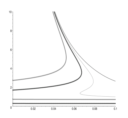
Figure 8: $h_{\infty}$ for solutions in a Minkowski ($\phi=0$) bulk. The thin-dark line has $\sigma=-2$, thin-light line has $\sigma=-1.2$, thick-dark lines have $\sigma=-1/2$ and the thick-light lines have $\sigma=2$.

In Fig. 8 we can see how solutions in each of the regions mentioned above affect $h_{\infty}$. The thin-dark line ($\sigma=-2$) lies in III and I in Fig. 6. Only GBIG2 exists for $0\leq\gamma<1/12$. For $\gamma>1/12$ we’ve seen that GBIG3 and GBIG2 connect to make a single solution, which is why the line is continuous through $\gamma=1/12$. The thin-light line ($\sigma=-1.2$) has an interesting feature due to the solutions lying on a line that cuts through both region III and IV as well as I. Both the thick lines have GBIG1-3 ending at $h_{\infty}$. The thick-dark solution loiters before evolving to $h_{\infty}$, but this has no effect upon the results in Fig. 8.

3.2 AdS bulk ($\phi\neq 0$) with brane tension

When $\phi=0$, we have $\Lambda_{5}\neq 0$, with one exception: the $\phi_{2}$ solution with $\chi=0$, i.e. $\phi_{2}=-4/3\gamma$, has $\Lambda_{5}=0$, but the bulk is AdS, Ref. Brown:2005ug . For $\chi>0$, $\Lambda_{5}\neq 0$. Thus in all cases, $\phi\neq 0$ implies an AdS bulk.

When we allow the bulk to be warped ($\phi\neq 0$) we open up another possible solution, denoted GBIG4. There is a maximum value of $\phi$ for which GBIG4 can exist as we shall see later. The nature of GBIG3 is also changed. These solutions, for a negative brane tension, can be seen in Fig. 9. Brane tension affects the solutions in the same manner as in $\phi=0$ case.

Figure 9: Solutions of the Friedmann equation ($h$ vs $\mu$) with negative brane tension ($\sigma=-2$) in an AdS bulk ($\phi=-0.1$) with $\gamma=1/20$. The curves are independent of the equation of state $w$. The arrows indicate the direction of proper time on the brane.

The qualitative effect of the warped bulk is to make GBIG3 collapse and to introduce the new bouncing branch GBIG4. This is due to $h=0$ now giving two solutions:

$$\mu_{\rm c,b}=\pm\sqrt{-\phi}\left(2+\gamma\phi\right)-\sigma,$$ (24)

where the plus sign is for the GBIG3 collapse ($\mu_{\rm c}$) and the minus for the GBIG4 bounce ($\mu_{\rm b}$). Effectively the loitering point in the Minkowski bulk is split into the max/min densities of the bouncing/collapsing cosmologies of GBIG3-4. The other points in Fig. 9 are modified by the warped bulk; they are now given by:

$$\mu_{\rm i,e}=\frac{1-18\gamma+27\gamma^{2}\phi\pm(1-12\gamma-18\gamma^{2}\phi)^{3/2}}{54\gamma^{2}}-\sigma,$$ (25)

with the plus sign for $\mu_{\rm i}$ and the negative sign for $\mu_{\rm e}$. The Hubble rates $h_{\rm i,e}$ are given by:

$$h_{\rm i,e}=\frac{\sqrt{2}}{6\gamma}\sqrt{1-6\gamma+9\gamma^{2}\phi\pm\sqrt{1-12\gamma-18\gamma^{2}\phi}},$$ (26)

with the same sign convention. $h_{\infty}$ is given by a similarly modified equation:

$$h_{\infty}^{6} + \frac{(8\gamma-1)}{4\gamma^{2}}h_{\infty}^{4}+\frac{[4+2\sigma-\phi\gamma(4+3\phi\gamma)]}{4\gamma^{2}}h_{\infty}^{2}$$ (27)

$$- \frac{\phi(2+\phi\gamma)^{2}+\sigma^{2}}{4\gamma^{2}}=0.$$

With a warped bulk the constraint from $h_{\rm i}$ ($\gamma\leq 1/12$ in the Minkowski case) is modified. In our equation for $h_{\rm i}$ we effectively have two bounds from the two square root terms. In the $\phi=0$ case only the inner term is of any consequence (giving rise to the bound $\gamma\leq 1/12$). When $\phi\neq 0$ there are two bounds which are applicable in different regimes. If we consider the bound from the inner square root we get:

$$\gamma\leq\frac{\sqrt{4+2\phi}-2}{6\phi}.$$ (28)

This is valid for $\phi\geq-2$. Considering the outer square root term we get the bound:

$$\gamma\leq\frac{2\left(1-\sqrt{-\phi}\right)}{3\phi}.$$ (29)

This bound becomes negative when $\phi>-1$ which is unallowed due to our string constraint. The bound on $\gamma$ is given by the lower of the two constraints when $-2<\phi<-1$ i.e. when in the range where both exists. Therefore the bound on $\gamma$ for $h_{\rm i}$ to be real is given by (see Fig. 10):

$$\gamma\leq\left\{\begin{array}[]{lc}\frac{\sqrt{4+2\phi}-2}{6\phi}&-\frac{16}{9}\leq\phi\leq 0\\ \\ \frac{2\left(1-\sqrt{-\phi}\right)}{3\phi}&\phi\leq-\frac{16}{9}\\ \end{array}\right.$$ (30)

Figure 10: In order for $h_{\rm i}$ to be real $\gamma$ must lie beneath the solid line ($\gamma_{\rm m}$). The region to the right of the vertical dotted line is where GBIG4 ($h_{\rm e}>0$) is allowed (except where $\phi=0$).

For a particular value of $\phi$ the maximum value of $\gamma$ allowed by this constraint is denoted $\gamma_{\rm m}$. When $\phi<-9$ the constraint in Eq. (12) is tighter than that in Eq. (29) ($\gamma_{\rm M}<\gamma_{\rm m}$). This means that for $\phi\leq-9$, $h_{\rm i}$ is always real for allowed values of $\gamma$.

There is a bound for GBIG4 to exist, found by considering $h_{\rm e}=0$. This bound is given by:

$$\phi>-\frac{2}{9\gamma^{2}}\left\{1-3\gamma-\sqrt{1-6\gamma}\right\}.$$ (31)

This is a solution to the quadratic obtained from $h_{\rm e}=0$, the other root of the quadratic does not obey the constraint $\phi\leq-4/3\gamma$ so is ignored. Using our constraints we can split the $\gamma,~{}\phi$ plane into three sections, see Fig. 10. The solid line is constructed from the bounds in Eq. (30). For $h_{\rm i}$ to be real we must choose values below this line. The area to the right of the vertical dotted line (but excluding $\phi=0$) allows GBIG4. Points to left of this line have GBIG1 collapsing after a minimum energy density ($\mu_{\rm b}$) is reached. The dotted curve on the left comes from initial constraint $\gamma\leq-4/3\phi$.

In order to consider the $\sigma,~{}\gamma$ plane as we did in the $\phi=0$ Minkowski case, we need the modified $\sigma_{\rm i,e}$ equations:

$$\sigma_{\rm i,e}=\frac{1-18\gamma+27\gamma^{2}\phi\pm(1-12\gamma-18\gamma^{2}\phi)^{3/2}}{54\gamma^{2}}.$$ (32)

We now have two more formulas for the collapse density of GBIG3 and the bounce density of GBIG4:

$$\sigma_{\rm c,b}=\pm\sqrt{-\phi}\left(2+\gamma\phi\right),$$ (33)

with the plus sign corresponding to the collapse and the minus to the bounce.

We shall consider the $\sigma,~{}\gamma$ plane for three different values of $\phi$ corresponding to three distinct regions in Fig. 10. We shall first consider $\phi=-1/2$.

3.2.1 Typical example $\phi=-1/2$

If we take $\phi=-1/2$, we are in the region where GBIG4 is allowed. The $\sigma,~{}\gamma$ plane can be seen in Fig. 11. The regions I, II and III in Fig. 11 extend up to $\gamma_{\rm M}=8/3$.

Figure 11: The $(\sigma,\gamma)$ plane for solutions in a AdS ($\phi=-1/2$) bulk. The short dotted horizontal line is the maximum value of $\gamma$ as obtained from Eq. (12).

In each region we have the following cosmologies.

• $I:~{}\sigma_{\rm e}(\gamma_{m})<\sigma<0,~{}\gamma>\gamma_{\rm i}$ and $\sigma\leq\sigma_{\rm e}(\gamma_{m}),~{}\gamma>\gamma_{\rm m}$. GBIG1-2 do not exist. GBIG3 reaches a minimum energy density ($\mu_{\rm c}$) and then evolves back to $\mu=\infty$. GBIG4 starts at ($0,-h_{\infty}$) then bounces at ($\mu_{\rm b},0$) before evolving to ($0,+h_{\infty}$). When $\sigma=\sigma_{\rm b}$ GBIG4 exists as a Minkowski universe.

• $II:~{}\sigma_{\rm b}\leq\sigma<\sigma_{\rm c},~{}\gamma>\gamma_{\rm i}$. GBIG1-2 and 4 do not exist. GBIG3 reaches a minimum energy density ($\mu_{\rm c}$) and then evolves back to $\mu=\infty$. When $\sigma=\sigma_{\rm c}$ GBIG3 ends in a Minkowski universe.

• $III:~{}\sigma>\sigma_{\rm c},~{}\gamma>\gamma_{\rm i}$. GBIG1-2 and 4 do not exist. GBIG3 evolves to a vacuum de Sitter universe.

• $IV:~{}\sigma\leq\sigma_{\rm e}<0,~{}\gamma\leq\gamma_{\rm m}$. GBIG1 evolves to ($\mu_{\rm e},h_{\rm e}$). GBIG2 evolves to $h_{\infty}$. GBIG3 reaches a minimum energy density ($\mu_{\rm c}$) and then evolves back to $\mu=\infty$. GBIG4 starts at ($\mu_{\rm e},-h_{\rm e}$), bounces at ($\mu_{\rm b},0$) before evolving to ($\mu_{\rm e},+h_{\rm e}$). When $\sigma=\sigma_{\rm e}$ GBIG1 and 3 evolve to ($0,h_{\rm e}$). GBIG4 starts at ($0,-h_{\rm e}$) and bounces before evolving to ($0,h_{\rm e}$). When $\gamma=\gamma_{\rm m}$ GBIG1 ceases to exist ($h_{\rm i}=h_{\rm e}$).

• $V:~{}\sigma_{\rm e}<\sigma\leq\sigma_{\rm b},~{}\gamma\leq\gamma_{\rm i}$. GBIG1-2 both end in vacuum de Sitter universes with different values of $h_{\infty}$. GBIG3 reaches a minimum energy density ($\mu_{\rm c}$) and then evolves back to $\mu=\infty$. GBIG4 starts at ($0,-h_{\infty}$) then bounces at ($\mu_{\rm b},0$) before evolving back to ($0,+h_{\infty}$). When $\sigma=\sigma_{\rm b}$ GBIG4 exists as a Minkowski universe ($0,0$).

• $VI:~{}\sigma_{\rm b}<\sigma\leq\sigma_{\rm c},~{}\gamma\leq\gamma_{\rm i}$. GBIG1-2 both end in vacuum de Sitter universes with different values of $h_{\infty}$. GBIG3 reaches a minimum energy density ($\mu_{\rm c}$) and then evolves back to $\mu=\infty$. GBIG4 does not exist. When $\sigma=\sigma_{\rm c}$ GBIG3 ends in a Minkowski universe. When $\gamma=\gamma_{\rm i}$ GBIG1-2 live at ($0,h_{\rm i}$).

• $VII:~{}\sigma>\sigma_{\rm c},~{}\gamma\leq\gamma_{\rm i}$. GBIG1-3 all end in vacuum de Sitter universes with different values of $h_{\infty}$. GBIG4 does not exist. When $\gamma=\gamma_{\rm i}$ GBIG1-2 live at ($0,h_{\rm i}$).

In region I there is a GBIG4 solution, which is modified in the same way as the GBIG3 solution in the Minkowski bulk. As $h_{\rm i,e}$ are no longer valid in region I GBIG4 joins onto GBIG2, see Fig. 12.

Figure 12: The GBIG4 solution in region I for $\phi=-1/2,\gamma=0.1>\gamma_{\rm m}$ and $\sigma=-2$. The bottom plot is $h^{\prime\prime}$ vs $\mu$ for this solution. This shows the differences between this solution and the similar case when $\phi=-4$, where GBIG4 is no longer allowed. Arrows denote proper time.

The bottom plot in this figure shows $h^{\prime\prime}$, in order to clearly distinguish this solution from the one in the $\phi=-4$ case where GBIG4 is no longer allowed.

In Fig. 13 are the results for $h_{\infty}$ with $\phi=-1/2$. The thin-dark line ($\sigma=-2$) lies in regions I and IV. Therefore we have only one solution for $h_{\infty}$, which corresponds to GBIG2 for $\gamma\leq\gamma_{\rm m}$. For $\gamma_{\rm m}<\gamma<\gamma_{\rm M}$ this root now corresponds to the end point for GBIG3 as in the $\phi=0$ case. The thin-light lines ($\sigma=-1.5$) lie in regions I and V. There are the two GBIG1-2 solutions and the GBIG4 solution which converges with the light-thick line at the bottom. The thick-dark line ($\sigma=0$) lies in regions II and VI, so only has GBIG1-2 present. The thick-light lines ($\sigma=2$) lie in regions III and VII, so has GBIG1-2 and the GBIG3 solution (the horizontal line).

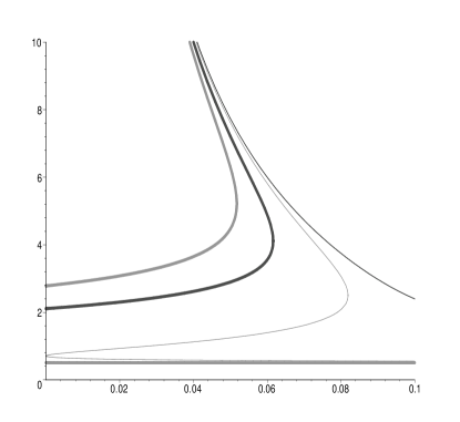
Figure 13: $h_{\infty}$ for solutions in a AdS ($\phi=-1/2$) bulk. The thin-dark line has $\sigma=-2$, thin-light lines have $\sigma=-1.5$, thick-dark line has $\sigma=0$ and the thick-light lines have $\sigma=2$.

3.2.2 Typical example: $\phi=-4$

We now consider $\phi=-4$ which is in the region where GBIG4 no longer exists (see Fig. 14), as $h_{\rm e}=0$.

Figure 14: Solutions of the Friedmann equation ($h$ vs $\mu$) with negative brane tension ($\sigma=-4$) in an AdS bulk ($\phi=-4$) with $\gamma=1/20$. For this value of $\phi$ GBIG4 no longer exists and GBIG1 can collapse. The curves are independent of the equation of state $w$. The arrows indicate the direction of proper time on the brane.

Therefore $\mu_{\rm e}$ is not relevant and GBIG1 bounces at $\mu_{\rm b}$. This means that the ($\sigma,~{}\phi$) plane, Fig. 15, is simpler.

Figure 15: The $(\sigma,\gamma)$ plane for solutions in a AdS ($\phi=-4$) bulk. The short dotted horizontal line is the maximum value of $\gamma$ as obtained from Eq. (28). The top horizontal line is from the initial bound in Eq. (10).

The regions in Fig. 15 are:

• $I:~{}\sigma\leq\sigma_{\rm b},~{}\gamma_{\rm m}<\gamma\leq\gamma_{\rm M}$. GBIG1 does not exist. GBIG2 starts at ($0,-h_{\infty}$), collapses to ($\mu_{\rm b},0$) and then expands back to ($0,h_{\infty}$). GBIG3 expands to ($\mu_{\rm c},0$) and then collapses. When $\sigma=\sigma_{\rm b}$ GBIG2 exists as a Minkowski universe.

• $II:~{}\sigma_{\rm b}<\sigma\leq\sigma_{\rm c},~{}\gamma_{\rm i}<\gamma\leq\gamma_{\rm M}$. GBIG1-2 do not exist. GBIG3 expands to $\mu_{\rm c}$ and then collapses. When $\sigma=\sigma_{\rm c}$ GBIG3 evolves to a Minkowski universe.

• $III:~{}\sigma>\sigma_{\rm c},~{}\gamma_{\rm i}<\gamma\leq\gamma_{\rm M}$. GBIG1-2 do not exist. GBIG3 evolves to $h_{\infty}$.

• $IV:~{}\sigma\leq\sigma_{\rm b},~{}\gamma\leq\gamma_{\rm m}$. GBIG1 evolves from $\mu_{\rm i}$ to $\mu_{\rm b}$ and then expands back to $\mu_{\rm i}$. GBIG2 evolves to $h_{\infty}$. GBIG3 expands to $\mu_{\rm c}$ and then collapses. When $\gamma=\gamma_{\rm m}$ GBIG1 ceases to exist, GBIG2 expands from ($\mu_{\rm b},0$). When $\sigma=\sigma_{\rm b}$ GBIG1 evolves to a Minkowski universe.

• $V:~{}\sigma_{\rm b}<\sigma\leq\sigma_{\rm c},~{}\gamma\leq\gamma_{\rm i}$. GBIG1-2 evolve to $h_{\infty}$. GBIG3 expands to $\mu_{\rm c}$ and then collapses. When $\gamma=\gamma_{\rm i}$ GBIG1-2 exist as the same de Sitter universe with ($0,h_{\infty}$). When $\sigma=\sigma_{\rm c}$ GBIG3 ends as a Minkowski universe.

• $VI:~{}\sigma>\sigma_{\rm c},~{}\gamma\leq\gamma_{\rm i}$. GBIG1-3 evolve to $h_{\infty}$. When $\gamma=\gamma_{\rm i}$ GBIG1-2 live at ($0,h_{\infty}$).

In region I we again have a combined solution as GBIG1 has vanished. As GBIG4 is not allowed ($h_{\rm e}=0$) when we take $\gamma>\gamma_{\rm m}$, which causes $h_{\rm i}=0$, GBIG2 matches up with its negative counterpart. We see the bouncing GBIG2 solution in Fig. 16. Note the nature of $h^{\prime\prime}$ is very different to that of the GBIG2, 4 bounce in the $\phi=-1/2$ case.

Figure 16: The GBIG4 solution in region I for $\phi=-4,\gamma=0.2>\gamma_{\rm m}$ and $\sigma=-4$. The bottom plot is $h^{\prime\prime}$ vs $\mu$ for this solution. This shows the differences between this solution and the case when $\phi=-1/2$. Arrows denote proper time.

In Fig. 17 we present results for $h_{\infty}$ for $\phi=-4$.

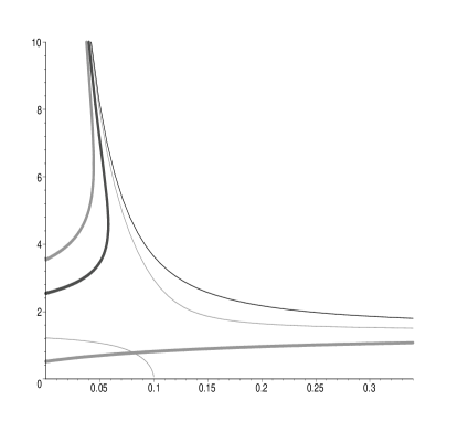
Figure 17: $h_{\infty}$ for solutions in a AdS ($\phi=-4$) bulk. The thin-dark line has $\sigma=-4.4$, thin-light lines have $\sigma=-3.2$, thick-dark line has $\sigma=0$ and the thick-light lines have $\sigma=4.4$.

3.2.3 Typical example: $\phi=-20$

Here we shall present results for $\phi=-20$ for completeness. This value of $\phi$ lives in the region of Fig. 10 where $h_{\rm i}$ is always real. This means that the $\sigma,~{}\gamma$ plane is much simpler, Fig. 18.

Figure 18: The $(\sigma,\gamma)$ plane for solutions in a AdS ($\phi=-20$) bulk. The top horizontal line is the bound from our initial bound in Eq. (10).

The regions in Fig. 18 are:

• $I:~{}\sigma\leq\sigma_{\rm b},~{}\gamma\leq\gamma_{\rm M}$. GBIG1 evolves from $\mu_{\rm i}$ to $\mu_{\rm b}$ and back. GBIG2 evolves to $h_{\infty}$. GBIG3 expands to $\mu_{\rm c}$ and then collapses. When $\sigma=\sigma_{\rm b}$ GBIG1 ends in a Minkowski universe.

• $II:~{}\sigma_{\rm i}<\sigma\leq\sigma_{\rm c},~{}\gamma_{\rm i}<\gamma\leq\gamma_{\rm M}$. GBIG1-2 do not exist. GBIG3 expands to $\mu_{\rm c}$ and then collapses. When $\sigma=\sigma_{\rm c}$ GBIG3 evolves to a Minkowski universe.

• $III:~{}\sigma>\sigma_{\rm c},~{}\gamma_{\rm i}<\gamma\leq\gamma_{\rm M}$. GBIG1-2 do not exist. GBIG3 evolves to $h_{\infty}$.

• $IV:~{}\sigma_{\rm b}<\sigma\leq\sigma_{\rm i}$ and $~{}\sigma_{\rm b}<\sigma\leq\sigma_{\rm c}$; $\gamma\leq\gamma_{\rm M}$ and $\gamma\leq\gamma_{\rm i}$. GBIG1-2 do not exist. GBIG3 expands to $\mu_{\rm c}$ and then collapses. When $\gamma=\gamma_{\rm i}$ (and for $\sigma=\sigma_{\rm i}$) GBIG1-2 both live at ($0,h_{\infty}$). When $\sigma=\sigma_{\rm c}$ GBIG3 evolves to a Minkowski universe.

• $V:~{}\sigma>\sigma_{\rm c},~{}\gamma\leq\gamma_{\rm i}$. GBIG1-3 evolve to $h_{\infty}$. When $\gamma=\gamma_{\rm i}$ GBIG1-2 both live at ($0,h_{\infty}$).

As we decrease the value of $\phi$, region II in Fig. 18 shrinks (the point $\sigma_{\rm i}(\gamma_{\rm M})$ becomes increasingly positive). For $\phi\leq-256/9$ region II no longer exists. The nature of the solutions in the other regions are unaffected.

There are no bouncing solutions in this case (in fact for any case with $\phi\leq-9$) as GBIG4 is unallowed and $\gamma_{\rm M}<\gamma_{\rm m}$ (which rules out the combined solutions). In Fig. 19 we show the $h_{\infty}$ results for $\phi=-20$.

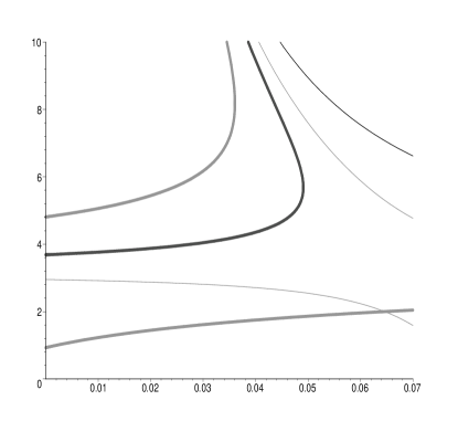
Figure 19: $h_{\infty}$ for solutions in a AdS ($\phi=-20$) bulk. The thin-dark line has $\sigma=-10$, thin-light lines have $\sigma=-2$, thick-dark lines has $\sigma=2$ and the thick-light lines has $\sigma=10$.

4 Conclusions

In this work we have looked at the general GBIG model. We have seen that there is a range of possible dynamics that can be achieved depending on the parameters in the model. Our main model of interest is still GBIG1 as this is the one that starts in a finite density “quiescent” singularity and evolves to a de Sitter universe. If we warp the bulk enough, GBIG1 can be allowed to collapse back to its initial density, provided there is sufficient negative brane tension. If the bulk is warped enough to allow GBIG1 to collapse this means that the bouncing cosmology GBIG4 can no longer exist. The exact nature of the late time dynamics can be changed by including a non-zero brane tension. A negative brane tension can reduce the Hubble rate at late time and a positive tension will increase it. GBIG1 can end in a future “quiescent” singularity with a non-zero density if we have an appropriate (negative) brane tension present. As the solution of interest is GBIG1 and we want it to provide the late time acceleration that we are experiencing it needs to end as a vacuum de Sitter universe. Therefore if there is some brane tension it must take values $\sigma_{\rm i}>\sigma>\sigma_{\rm e}$.

GBIG2 also starts in a “quiescent” singularity but it super-accelerates so is un-physical and of little interest.

GBIG3 still starts in an infinite density big-bang but has a number of possible late time dynamics. In a Minkowski bulk GBIG3 can either evolve to a Minkowski state, as shown in Ref. Brown:2005ug , a vacuum de Sitter state or even loiter around $\mu=-\sigma$ before ending in a vacuum de Sitter state or a “quiescent” singularity. This loitering cosmology is different from that in Ref. Sahni:2004fb , as we do not require a naked bulk singularity or a de Sitter bulk. If we warp the bulk GBIG3, will generally collapse, unless there is sufficient (positive) brane tension to allow the solution to end in a vacuum de Sitter state.

GBIG4 can only ever exist in a mildly warped bulk with negative brane tension. So it can be said that GBIG4 is un-physical due to requirement that $\sigma<0$.

There are a number of bouncing cosmologies within this set-up. There are the GBIG4 solutions as mentioned above. There are also the solutions where GBIG4 and 2 match up ($\gamma_{\rm m}<\gamma\leq\gamma_{\rm M}$ with $\phi_{\rm GBIG4Lim}<\phi<0$) and the GBIG2 bouncing cosmologies ($\gamma_{\rm m}<\gamma\leq\gamma_{\rm M}$ with $-9<\phi\leq\phi_{\rm GBIG4Lim}$). Each of these have different dynamics so would produce different evolutionary histories. The solutions that spend time on the GBIG2 branch will experience phantom like behaviour during this period.

Acknowledgements: I am supported by PPARC. I thank Roy Maartens and Mariam Bouhmadi-Lopez and for very helpful discussions. I would also like to thank Varun Sahni for pointing out Ref. Shtanov:2002ek .

References

- (1) G. R. Dvali, G. Gabadadze and M. Porrati, “4D gravity on a brane in 5D Minkowski space,” Phys. Lett. B 485, 208 (2000) [arXiv:hep-th/0005016].
- (2) C. Deffayet, “Cosmology on a brane in Minkowski bulk,” Phys. Lett. B 502, 199 (2001) [arXiv:hep-th/0010186].
- (3) N. E. Mavromatos and E. Papantonopoulos, “Induced curvature in brane worlds by surface terms in string effective actions with higher-curvature corrections,” Phys. Rev. D 73 (2006) 026001 [arXiv:hep-th/0503243].
- (4) See, e.g., J. E. Kim, B. Kyae and H. M. Lee, “Various modified solutions of the Randall-Sundrum model with the Gauss-Bonnet interaction,” Nucl. Phys. B 582 (2000) 296 [Erratum-ibid. B 591 (2000) 587] [arXiv:hep-th/0004005]; Y. M. Cho and I. P. Neupane, “Warped brane-world compactification, black hole thermodynamics and holographic cosmology with R**2 terms,” Int. J. Mod. Phys. A 18 (2003) 2703 [arXiv:hep-th/0112227]; C. Charmousis and J. F. Dufaux, “General Gauss-Bonnet brane cosmology,” Class. Quant. Grav. 19, 4671 (2002) [arXiv:hep-th/0202107]; S. Nojiri, S. D. Odintsov and S. Ogushi, “Friedmann-Robertson-Walker brane cosmological equations from the five-dimensional bulk (A)dS black hole,” Int. J. Mod. Phys. A 17, 4809 (2002) [arXiv:hep-th/0205187]; S. C. Davis, “Generalised Israel junction conditions for a Gauss-Bonnet brane world,” Phys. Rev. D 67, 024030 (2003) [arXiv:hep-th/0208205]; E. Gravanis and S. Willison, “Israel conditions for the Gauss-Bonnet theory and the Friedmann equation on the brane universe,” Phys. Lett. B 562, 118 (2003) [arXiv:hep-th/0209076]; J. E. Lidsey and N. J. Nunes, “Inflation in Gauss-Bonnet brane cosmology,” Phys. Rev. D 67, 103510 (2003) [arXiv:astro-ph/0303168]; K. i. Maeda and T. Torii, “Covariant gravitational equations on brane world with Gauss-Bonnet term,” Phys. Rev. D 69, 024002 (2004) [arXiv:hep-th/0309152]; M. Sami and V. Sahni, “Quintessential inflation on the brane and the relic gravity wave background,” Phys. Rev. D 70 (2004) 083513 [arXiv:hep-th/0402086]; S. Tsujikawa, M. Sami and R. Maartens, “Observational constraints on braneworld inflation: The effect of a Gauss-Bonnet term,” Phys. Rev. D 70 (2004) 063525 [arXiv:astro-ph/0406078]; S. Nojiri and S. D. Odintsov, “Is brane cosmology predictable?,” Gen. Rel. Grav. 37 (2005) 1419 [arXiv:hep-th/0409244]; T. G. Rizzo, “Warped phenomenology of higher-derivative gravity,” JHEP 0501, 028 (2005) [arXiv:hep-ph/0412087].
- (5) L. Randall and R. Sundrum, “An alternative to compactification,” Phys. Rev. Lett. 83, 4690 (1999) [arXiv:hep-th/9906064].
- (6) See, e.g., E. Kiritsis, N. Tetradis and T. N. Tomaras, “Induced gravity on RS branes,” JHEP 0203 (2002) 019 [arXiv:hep-th/0202037]; T. Tanaka, “Weak gravity in DGP braneworld model,” Phys. Rev. D 69, 024001 (2004) [arXiv:gr-qc/0305031]; E. Papantonopoulos and V. Zamarias, “Chaotic inflation on the brane with induced gravity,” JCAP 0410, 001 (2004) [arXiv:gr-qc/0403090].
- (7) G. Kofinas, R. Maartens and E. Papantonopoulos, “Brane cosmology with curvature corrections,” JHEP 0310, 066 (2003) [arXiv:hep-th/0307138].
- (8) R. G. Cai, H. S. Zhang and A. Wang, “Crossing w = -1 in Gauss-Bonnet brane world with induced gravity,” Commun. Theor. Phys. 44 (2005) 948 [arXiv:hep-th/0505186].
- (9) R. A. Brown, R. Maartens, E. Papantonopoulos and V. Zamarias, “A late-accelerating universe with no dark energy - and a finite-temperature big bang,” JCAP 0511, 008 (2005) [arXiv:gr-qc/0508116].
- (10) J. F. Dufaux, J. E. Lidsey, R. Maartens and M. Sami, “Cosmological perturbations from brane inflation with a Gauss-Bonnet term,” Phys. Rev. D 70, 083525 (2004) [arXiv:hep-th/0404161].
- (11) Y. Shtanov and V. Sahni, “Unusual cosmological singularities in braneworld models,” Class. Quant. Grav. 19 (2002) L101 [arXiv:gr-qc/0204040].
- (12) V. Sahni and Y. Shtanov, “Did the Universe loiter at high redshifts ?,” Phys. Rev. D 71 (2005) 084018 [arXiv:astro-ph/0410221].