The number of negative modes of the oscillating bounces

Abstract

The spectrum of small perturbations about oscillating bounce solutions recently discussed in the literature is investigated. Our study supports quite intuitive and expected result: the bounce with $N$ nodes has exactly $N$ homogeneous negative modes. Existence of more than one negative modes makes obscure the relation of these oscillating bounce solutions to the false vacuum decay processes.

I Introduction

Having in mind recent progress in string theory, predicting string landscape (many vacua) picture, it is very important to have deeper understanding of metastable vacuum decay processes with gravity taken into account. Metastable (false) vacuum decay is a quantum tunnelling process and is usually described within the Euclidean approach col77 . It was shown that the metastable vacuum decay in flat space-time proceeds via true vacuum bubbles nucleation in the false vacuum and subsequent growth of these bubbles. Bubble nucleation process is described by bounce, classical solution of the Euclidean equations of motion with certain boundary conditions. It was found coglma78 that in flat space-time the $O(4)-$ symmetric bounce has lowest action and gives main contribution to the tunnelling. Furthermore, it was shown that there is exactly one negative mode in spectrum of small perturbations about bounce solution in flat space-time caco77 . This negative mode is very essential and makes decay picture coherent. In Coleman’s words: “There may exist solutions in other ways like bounces and which have more than one negative eigenvalue, but, even if they do exist, they have nothing to do with tunnelling” col88 .

Bounce solution in presence of gravity was found by Coleman and De Luccia colu80 . In addition some exited multi bounce solutions are known in the literature: Bousso and Linde discussed double-bubble instantons bl98 and more recently the oscillating bounce solutions were studied in details by Hackworth and Weinberg hw05 ; wein05 . It was found that multi bounces have higher Euclidean action than the bounce itself. So, it was suggested that the multi bounces give sub-leading contribution to the vacuum decay processes.

The aim of the present letter is to investigate the number of negative modes of these oscillating bounce solutions in order to check their relevance to the tunnelling. While in flat space-time finding a negative mode about bounce is straightforward task, when gravity is taken into account it is more involved problem lrt85 ; tasa92 ; lav98 ; tanaka99 ; klt00 ; lav00 ; grtu01 . It was shown that with the proper reduction procedure one finds a single negative mode about Coleman-De Luccia bounce klt00 .

The rest of the paper is organized as follows: in the next section we discuss the Euclidean equations of motion and boundary conditions for the bounce solution. In Section III we present Schröedinger equation for linear perturbations about the bounce and in the Section IV be show out numerical results for concrete choice of scalar field potentials.

II Bounce solution

Let’s consider the theory of a scalar field coupled to gravity which is defined by the following Euclidian action

$$S_{E}=\int{d^{4}x\sqrt{g}\;\Bigl{(}\frac{1}{2}\nabla_{\mu}\phi\nabla^{\mu}\phi+V(\phi)-\frac{1}{2\kappa}R\Bigr{)}}\;,$$ (1)

where $\kappa=8\pi G_{N}$ is the reduced Newton’s gravitational constant.

The most general $O(4)$ invariant metric is parameterized as

$$ds^{2}=N^{2}(\sigma)d\sigma^{2}+a^{2}(\sigma)d\Omega_{3}^{2}\;,$$ (2)

where $N(\sigma)$ is the Lapse function, $a(\sigma)$ is the scale factor and $d\Omega_{3}^{2}$ is metric of unit three-sphere:

$$d\Omega_{3}^{2}=d\chi^{2}+{\rm sin}^{2}\chi(d\theta^{2}+{\rm sin}^{2}(\theta)d\varphi^{2})\;.$$ (3)

For metric Eq. (2) the curvature scalar looks like

$$R=\frac{6}{a^{2}}-\frac{6\dot{a}^{2}}{a^{2}N^{2}}-\frac{6\ddot{a}}{aN^{2}}+\frac{6\dot{a}\dot{N}}{aN^{3}}\;,$$ (4)

where $\dot{}=d/d\sigma$. Using ansatz Eq. (2) and assuming that $\phi=\phi(\sigma)$ we get the reduced action in the form

$$S_{E}=S_{E}(\phi,N,a)=2\pi^{2}\int d\sigma\Bigl{(}\frac{a^{3}}{2N}\dot{\phi}^{2}+a^{3}NV(\phi)-\frac{3aN}{\kappa}+\frac{3a\dot{a}^{2}}{\kappa N}+\frac{3a^{2}\ddot{a}}{\kappa N}-\frac{3a^{2}\dot{a}\dot{N}}{\kappa N^{2}}\Bigr{)}\;.$$ (5)

Corresponding field equations in the proper time gauge, $N=1$, are

$$\ddot{\phi}+3\frac{\dot{a}}{a}\dot{\phi}=\frac{\partial V}{\partial\phi}\;,$$ (6)

$$\ddot{a}=-\frac{\kappa a}{3}(\dot{\phi}^{2}+V(\phi))\;,$$ (7)

$$\dot{a}^{2}=1+\frac{\kappa a^{2}}{3}(\frac{\dot{\phi}^{2}}{2}-V)\;.$$ (8)

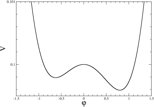
Now let’s assume that potential $V(\phi)$ has two non-degenerate local minima at $\phi=\phi_{\rm tr}$ and $\phi=\phi_{\rm fv}$, with $V(\phi_{\rm fv})>V(\phi_{\rm tr})$, and local maximum for some $\phi=\phi_{\rm top}$, with $\phi_{\rm fv}<\phi_{\rm top}<\phi_{\rm tv}$, Fig. 1. Euclidean solution describing vacuum decay - bounce - satisfies these equations and in case $V(\phi)>0$ has following boundary conditions

$$\phi(0)=\phi_{0},\qquad\dot{\phi}(0)=0,\qquad a(0)=0,\qquad\dot{a}(0)=1\;,$$ (9)

at $\sigma=0$ and

$$\phi(\sigma_{max})=\phi_{m},\qquad\dot{\phi}(\sigma_{max})=0,\qquad a(\sigma_{max})=0,\qquad\dot{a}(\sigma_{max})=1\;,$$ (10)

at some $\sigma=\sigma_{max}$. This assumes the following Taylor series at $\sigma\to 0$

$$\phi(\sigma)=\phi_{0}+\frac{1}{8}{\frac{\partial V}{\partial\phi}}|_{\phi=\phi_{0}}\sigma^{2}+\frac{1}{192}\frac{\partial V}{\partial\phi}|_{\phi=\phi_{0}}(\frac{\partial^{2}V}{\partial\phi^{2}}|_{\phi=\phi_{0}}+\frac{2\kappa V(\phi_{0})}{3})\sigma^{4}+O(\sigma^{6})\;,$$ (11)

$$a(\sigma)=\sigma-\frac{\kappa}{18}V(\phi_{0})\sigma^{3}-\frac{\kappa}{120}(\frac{3}{8}(\frac{\partial V}{\partial\phi}|_{\phi=\phi_{0}})^{2}-\frac{\kappa}{9}V^{2}(\phi_{0}))\sigma^{5}+O(\sigma^{7})\;,$$ (12)

and similar power law behavior for non-singular bounces for $x\to 0$, where $x=\sigma_{max}-\sigma$.

Whereas bounce solution always exists in the flat space-time, when gravity is switched on, the existence of bounce depends on details of scalar field potential. For wide class of potentials the existence of bounce solution is determined by the value of parameter $\beta$ js89 ,

$$\beta=|V^{\prime\prime}(\phi_{\rm top})|/H^{2}\;,$$ (13)

where $H^{2}={\kappa V(\phi_{\rm top})}/{3}$. For $\beta<4$ no Coleman-De Luccia bounce exists in the given potential. Increasing $\beta$ more and more oscillating bounce solutions appear. For broad class of potentials for a given $\beta$ there are oscillating bounces with up $N$ nodes, where $N$ is the largest integer such that $N(N+3)<\beta$ hw05 . In addition one finds also the Hawking-Moss solution hm82 which exist in any potential with positive local maximum.

III Linear perturbations

The investigation of perturbations about the bounce solution is convenient to perform in conformal frame klt00 ; lav00 . Let’s expand the metric and the scalar field over a $O(4)-$ symmetric background as follows

$$ds^{2}=a(\tau)^{2}\Bigl{(}(1+2A(\tau))d\tau^{2}+(1-2\Psi(\tau))d\Omega_{3}^{2}\Bigr{)}\;,\qquad\phi=\varphi(\tau)+\Phi(\tau)\;,$$ (14)

where $\tau$ is the conformal time, $a$ and $\varphi$ are the background field values and $A,\Psi$ and $\Phi$ are small perturbations. In what follows we will be interested in the lowest (only $\tau$ dependant, ‘homogeneous’) modes and consider only scalar metric perturbations, while the negative energy states are found previously exactly in this sector.

Expanding the total action, keeping terms up to the second order in perturbations and using the background equations of motion we find

$$S=S^{(0)}[a,\varphi]+S^{(2)}[A,\Psi,\Phi]\;,$$ (15)

where $S^{(0)}$ is the action of the background solution and $S^{(2)}[A,\Psi,\Phi]$ is the quadratic action. The Lagrangian corresponding to this quadratic action is degenerate and describes constrained dynamical system. Applying Dirac’s formulation of generalized Hamiltonian dynamics we get unconstrained quadratic action in the form klt00 ; lav00

$$S^{(2)}_{E}=2\pi^{2}\int\Bigl{(}\frac{1}{2}q^{\prime 2}+\frac{1}{2}W[a(\tau),\varphi(\tau)]\;q^{2}\Bigr{)}d\tau\;,$$ (16)

with the potential $W$ whose conformal time dependance is determined by the bounce solution lav00

$$W[a(\tau),\varphi(\tau)]=\frac{a^{2}}{\cal Q}\frac{\delta^{2}V}{\delta\varphi\delta\varphi}-\frac{10{a^{\prime}}^{2}}{a^{2}\cal Q}+\frac{12{a^{\prime}}^{2}}{a^{2}{\cal Q}^{2}}+\frac{8}{\cal Q}-6-3{\cal Q}+\frac{\kappa a^{4}}{2{\cal Q}^{2}}(\frac{\delta V}{\delta\varphi})^{2}-\frac{2\kappa aa^{\prime}\varphi^{\prime}}{{\cal Q}^{2}}\frac{\delta V}{\delta\varphi}\;.$$ (17)

Here $q=a/\sqrt{\cal Q}\;\Phi$, prime denotes the derivative with respect to conformal time $\tau$ and ${\cal Q}=1-\kappa\varphi^{\prime 2}/6$.

Introducing new variable $f=\sqrt{a}q$ and passing to the proper time $\sigma$ quadratic action Eq. (16) can be written in the form

$$S^{(2)}_{E}=2\pi^{2}\int\Bigl{(}\frac{1}{2}\dot{f}^{2}+\frac{1}{2}U[a(\sigma),\varphi(\sigma)]\;f^{2}\Bigr{)}d\sigma\;,$$ (18)

with the potential $U$

$$U[a(\sigma),\varphi(\sigma)]=\frac{1}{Q}\frac{\delta^{2}V}{\delta\varphi\delta\varphi}-\frac{10{\dot{a}}^{2}}{a^{2}Q}+\frac{12{\dot{a}}^{2}}{a^{2}Q^{2}}+\frac{8}{a^{2}Q}-\frac{6}{a^{2}}-\frac{3Q}{a^{2}}-\frac{{\dot{a}}^{2}}{4a^{2}}+\frac{\kappa a^{2}}{2Q^{2}}(\frac{\delta V}{\delta\varphi})^{2}-\frac{2\kappa a{\dot{a}}{\dot{\varphi}}}{Q^{2}}\frac{\delta V}{\delta\varphi}-\frac{\kappa}{6}(\dot{\varphi}^{2}+V),$$ (19)

where $Q=1-\kappa a^{2}{\dot{\varphi}}^{2}/6$. So, spectrum of small perturbations about bounce solution is determined by the following Schrödinger equation

$$-\frac{d^{2}}{d\sigma^{2}}f+U[a(\sigma),\varphi(\sigma)]f=Ef,$$ (20)

and the number of negative modes of the bounce solution is the number of bound states of these Schrödinger equation.

IV Numerical results

Let’s parameterize the general quartic scalar field potential as follows:

$$V=V_{0}+H^{2}(-\frac{\beta}{2}\varphi^{2}-\frac{g}{3}\varphi^{3}+\frac{\lambda}{4}\varphi^{4})\;,$$ (21)

with $H^{2}=\kappa V_{0}/3$.

Passing to the dimensionless variables

$$\tilde{\varphi}=\frac{\varphi}{v}\;,\tilde{a}=av\;,\tilde{\sigma}=\sigma v\;,\tilde{V}_{0}=\frac{V_{0}}{v^{4}}\;,\tilde{H}^{2}=\frac{H^{2}}{v^{2}}\;,\tilde{\kappa}=\kappa v^{2}\;,$$ (22)

with $v^{2}={2\beta}/{\lambda}$ we will get the dimensionless equations of motion with the rescaled potential (comp. hw05 )

$$\tilde{V}=\tilde{V}_{0}+\tilde{H}^{2}\beta(-\frac{1}{2}\tilde{\varphi}^{2}-\frac{\tilde{g}}{3}\tilde{\varphi}^{3}+\frac{1}{2}\tilde{\varphi}^{4})\;,$$ (23)

where $\tilde{g}=gv/\beta$. In what follows we will use dimensionless variables and omit tildes.

Potential $U$ close to the $\sigma=0$ behaves as

$$U=\frac{3}{4\sigma^{2}}+U_{0}+O(\sigma^{2})\;,$$ (24)

where constant $U_{0}$ depends on the initial value of scalar field and parameters of the background solution potential $V$. For the potential Eq. (23) it is

$$U_{0}=(-H^{2}\beta-\frac{2}{3}\kappa V_{0}-2H^{2}\beta g\phi_{0}+6H^{2}\beta(1+\frac{\kappa}{18})\phi_{0}^{2}+\frac{2}{9}\kappa H^{2}\beta g\phi_{0}^{3}-\frac{1}{3}\kappa H^{2}\beta\phi_{0}^{4})\;.$$ (25)

The regular branch of the wave function $f$ behaves as

$$f=\sigma^{3/2}(1+\frac{1}{8}(U_{0}-E)\sigma^{2}+O(\sigma^{4}))\;.$$ (26)

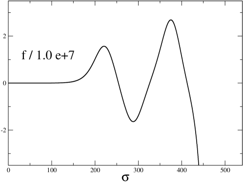
Convenient way to determine the number of bound states of Schrödinger equation in a given potential is the investigation of the zero energy wave function. The number of nodes of zero energy wave function exactly counts the number of negative energy states aq95 .

Let’s describe our results in details on concrete example. For the parameters choice

$$\kappa=0.001\;,V_{0}=0.1\;,\beta=70.03\;,g=\frac{1}{2\sqrt{2}}\;,$$ (27)

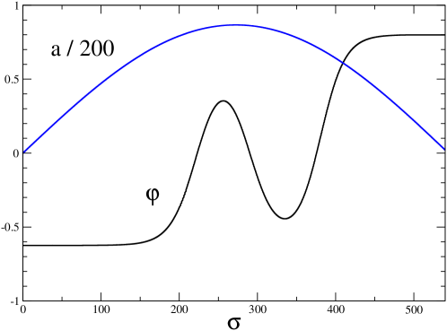
the potential Eq.(23) has local maximum at $\varphi_{\rm top}=0$, metastable minimum at $\varphi_{\rm fv}=-0.6242212930$ and true vacuum at $\varphi_{\rm tv}=0.8009979884$, Fig. 1. There exists Coleman-De Luccia bounce solution in this potential, oscillating bounces on top of it with up to $N=7$ nodes and, as always, the Hawking-Moss solution hm82 with $\varphi\equiv\varphi_{\rm top}$. Numerical investigation supports quite intuitive and expected result grtu01 : the bounce with $N$ nodes has exactly $N$ negative modes. Typical results are demonstrated for $N=3$ case on Fig.2 and Fig.3. The zero energy wave function of Schröedinger equation Eq. (20) has in this case three nodes, which means that there are exactly three negative energy states for $N=3$ oscillating bounce. We also found this states explicitly and determined their energies: $E_{0}=-0.0013787$, $E_{1}=-0.0004362$ and $E_{2}=-0.0001207$. Corresponding Hawking-Moss solution has eight homogeneous negative modes, which is consistent with chosen value of $\beta$.

To conclude, we found that the oscillating bounces studied in bl98 and hw05 have more than one negative modes, which makes their relevance to the tunnelling processes obscure. So, question about contribution of oscillating bounces to the false vacuum decay amplitude needs further investigation.

Figure 1: Scalar field potential $V(\varphi)$.

Figure 2: Oscillating bounce solution with three nodes of $\varphi$.

Figure 3: Zero energy wave function $f$ of Schrödinger equation of linear perturbations about oscillating bounce solution with three nodes of $\varphi$.

References

- (1) S. R. Coleman, “The Fate Of The False Vacuum. 1. Semiclassical Theory,” Phys. Rev. D 15 (1977) 2929 [Erratum-ibid. D 16 (1977) 1248].
- (2) S. R. Coleman, V. Glaser and A. Martin, “Action Minima Among Solutions To A Class Of Euclidean Scalar Field Equations,” Commun. Math. Phys. 58 (1978) 211.
- (3) C. G. . Callan and S. R. Coleman, “The Fate Of The False Vacuum. 2. First Quantum Corrections,” Phys. Rev. D 16 (1977) 1762.
- (4) S. R. Coleman, “Quantum Tunneling And Negative Eigenvalues,” Nucl. Phys. B 298 (1988) 178.
- (5) S. R. Coleman and F. De Luccia, “Gravitational Effects On And Of Vacuum Decay,” Phys. Rev. D 21 (1980) 3305.
- (6) R. Bousso and A. D. Linde, “Quantum creation of a universe with Omega not = 1: Singular and non-singular instantons,” Phys. Rev. D 58 (1998) 083503 [arXiv:gr-qc/9803068].
- (7) J. C. Hackworth and E. J. Weinberg, “Oscillating bounce solutions and vacuum tunneling in de Sitter spacetime,” Phys. Rev. D 71 (2005) 044014 [arXiv:hep-th/0410142].
- (8) E. J. Weinberg, “New bounce solutions and vacuum tunneling in de Sitter spacetime,” AIP Conf. Proc. 805 (2006) 259 [arXiv:hep-th/0512332].
- (9) G. Lavrelashvili, V. A. Rubakov and P. G. Tinyakov, “Tunneling Transitions With Gravitation: Breaking Of The Quasiclassical Approximation,” Phys. Lett. B 161 (1985) 280.
- (10) T. Tanaka and M. Sasaki, “False vacuum decay with gravity: Negative mode problem,” Prog. Theor. Phys. 88 (1992) 503.
- (11) G. Lavrelashvili, “On the quadratic action of the Hawking-Turok instanton,” Phys. Rev. D 58 (1998) 063505 [arXiv:gr-qc/9804056].
- (12) T. Tanaka, “The no-negative mode theorem in false vacuum decay with gravity,” Nucl. Phys. B 556 (1999) 373 [arXiv:gr-qc/9901082].
- (13) A. Khvedelidze, G. Lavrelashvili and T. Tanaka, “On cosmological perturbations in closed FRW model with scalar field and false vacuum decay,” Phys. Rev. D 62 (2000) 083501 [arXiv:gr-qc/0001041].
- (14) G. Lavrelashvili, “Negative mode problem in false vacuum decay with gravity,” Nucl. Phys. Proc. Suppl. 88 (2000) 75 [arXiv:gr-qc/0004025].
- (15) S. Gratton and N. Turok, “Homogeneous modes of cosmological instantons,” Phys. Rev. D 63 (2001) 123514 [arXiv:hep-th/0008235].
- (16) L. G. Jensen and P. J. Steinhardt, “Bubble Nucleation And The Coleman-Weinberg Model,” Nucl. Phys. B 237 (1984) 176; “Bubble Nucleation For Flat Potential Barriers,” Nucl. Phys. B 317 (1989) 693.
- (17) S. W. Hawking and I. G. Moss, “Supercooled Phase Transitions In The Very Early Universe,” Phys. Lett. B 110 (1982) 35.
- (18) H. Amann, P. Quittner, “A nodal theorem for coupled systems of Schrödinger equations and the number of bound states,” J. Math. Phys. 36 (1995) 2110.