Two-dimensional approach to relativistic positioning systems

Abstract

A relativistic positioning system is a physical realization of a coordinate system consisting in four clocks in arbitrary motion broadcasting their proper times. The basic elements of the relativistic positioning systems are presented in the two-dimensional case. This simplified approach allows to explain and to analyze the properties and interest of these new systems. The positioning system defined by geodesic emitters in flat metric is developed in detail. The information that the data generated by a relativistic positioning system give on the space-time metric interval is analyzed, and the interest of these results in gravimetry is pointed out.

I Introduction

In Astronomy, Space physics and Earth sciences, the increase in the precision of space and time localization of events is associated with the increase of a better knowledge of the physics involved. Up to now all time scales and reference systems, although incorporating so called ‘relativistic effects’ in their development, start from Newtonian conceptions.

In Relativity, the space-time is modeled by a four-dimensional manifold. In this manifold, most of the coordinates are usually chosen in order to simplify mathematical operations, but some of them, in fact a little set, admit more or less simple physical interpretations. What this means is that some of the ingredients of such coordinate systems (some of their coordinate lines, surfaces or hypersurfaces) may be imagined as covered by some particles, clocks, rods or radiations submitted to particular motions. But the number of such physically interpretable coordinate systems that can be physically constructed in practice is strongly limited.

In fact, among the at present physically interpretable coordinate systems, the only one that may be generically constructed is the one based in the Poincaré-Einstein protocol of synchronization, also called radar system. Unfortunately, this protocol suffers from the bad property of being a retarded protocol (see below).

Consequently, in order to increase our knowledge of the physics involved in phenomena depending on the space-time localization of their constituents, it is important to learn to construct physically good coordinate systems of relativistic quality.

To clearly differentiate the coordinate system as a mathematical object from its realization as a physical object, it is convenient to characterize this physical object with a proper name. For this reason, the physical object obtained by a peculiar materialization of a coordinate system is called a location system coll-1 ; coll-tarantola ; coll-3 . A location system is thus a precise protocol on a particular set of physical fields allowing to materialize a coordinate system.

A location system may have some specific properties coll-1 ; coll-3 . Among them, the more important ones are those of being generic, i.e. that can be constructed in any space-time of a given class, (gravity-)free, i.e. that the knowledge of the gravitational field is not necessary to construct it, and immediate, i.e. that every event may know its coordinates without delay. Thus, for example, location systems based in the Poincaré-Einstein synchronization protocol (radar systems) are generic and free, but not immediate.

Location systems are usually used either to allow a given observer assigning coordinates to particular events of his environment or to allow every event of a given environment to know its proper coordinates. Location systems constructed for the first of these two functions, following their three-dimensional Newtonian analogues, are called (relativistic) reference systems. In relativity, where the velocity of transmission of information is finite, they are necessarily not immediate. Poincaré-Einstein location systems are reference systems in the present sense.

Location systems constructed for the second of these two functions which, in addition, are generic, free and immediate, are called coll-1 (relativistic) positioning systems. Since Poincaré-Einstein reference systems are the only known location systems but they are not immediate, the first question is if in relativity there exist positioning systems having the three demanded properties of being generic, free and immediate. The epistemic answer is that there exists a little number of them, their paradigmatic representative being constituted by four clocks broadcasting their proper times.

In Newtonian physics, when the velocity of transmission of information is supposed infinite, both functions, of reference and positioning, are exchangeable in the sense that data obtained from any of the two systems may be transformed in data for the other one. But this is no longer possible in relativity, where the immediate character of positioning systems and the intrinsically retarded character of reference systems imposes a strong decreasing hierarchy.

Consequently, in relativity the experimental or observational context strongly conditions the function, conception and construction of location systems. In addition, by their immediate character, it results that whenever possible, there are positioning systems, and not reference systems, which offer the most interest to be constructed.

What is the coordinate system physically realized by four clocks broadcasting their proper time? Every one of the four clocks $\gamma_{i}$ (emitters) broadcasting his proper time $\tau^{i},$ the future light cones of the points $\gamma_{i}(\tau^{i})$ constitute the coordinate hypersurfaces $\tau^{i}=constant$ of the coordinate system for some domain of the space-time. At every event of the domain, four of these cones, broadcasting the times $\tau^{i},$ intersect, endowing thus the event with the coordinate values $\{\tau^{i}\}.$ In other words, the past light cone of every event cuts the emitter world lines at $\gamma_{i}(\tau^{i})$; then $\{\tau^{i}\}$ are the emission coordinates of this event.

Let $\gamma$ be an observer equipped with a receiver allowing the reception of the proper times $(\tau^{i})$ at each point of his trajectory. Then, this observer knows his trajectory in these emission coordinates. We say then that this observer is a user of the positioning system. It is worth pointing out that a user could, eventually (but not necessary), carry a clock to measure his proper time $\tau$.

A positioning system may be provided with the important quality of being auto-locating. For this goal, the emitters have also to be transmitters of the proper time they just receive, so that at every instant they must broadcast their proper time and also these other received proper times. Then, any user does not only receive the emitted times $\{\tau^{i}\}$ but also the twelve transmitted times $\{\tau^{i}_{j}\}$. These data allow the user to know the trajectories of the emitter clocks in emission coordinates.

The interest, characteristics and good qualities of the relativistic positioning systems have been pointed out elsewhere coll-1 ; coll-2 ; coll-3 and some explicit results have been recently presented for the generic four-dimensional case coll-pozo ; pozo . A full development of the theory for this generic case requires a hard task and a previous training on simple and particular examples. The two-dimensional approach that we present here should help to better understand how these systems work as well as the richness of the physical elements that this positioning approach has.

Indeed, the two-dimensional case has the advantage of allowing the use of precise and explicit diagrams which improve the qualitative comprehension of the general four-dimensional positioning systems. Moreover, two-dimensional constructions admit simple and explicit analytic results.

It is worth remarking that the two-dimensional case has some particularities and results that cannot be directly extended to the generic four-dimensional case. Two dimensional constructions are suitable for learning basic concepts about positioning systems, but they do not allow to study some positioning features that necessarily need a three-dimensional or a four-dimensional approach.

As already mentioned, the coordinate system that a positioning system realizes is constituted by four null (one-parametric family of) hypersurfaces, so that its covariant natural frame is constituted by four null 1-forms. Such rather unusual real null frames belong to the causal class $\{\,{\rm e}{\rm e}{\rm e}{\rm e}\,,\,{\rm E}{\rm E}{\rm E}{\rm E}{\rm E}{\rm E}\,,\,\ell\ell\ell\ell\,\}$ of frames among the 199 admitted by a four-dimensional Lorentzian metric coll-morales ; moralesERE05 . Up to recently, and all applications taken into account, this causal class, or its algebraically dual one, $\{\,{\rm l}{\rm l}{\rm l}{\rm l}\,,\,{\rm T}{\rm T}{\rm T}{\rm T}{\rm T}{\rm T}\,,\,eeee\,\},$ has been considered in the literature but very sparingly.

Zeeman Zeeman seems the first to have used, for a technical proof, real null frames, and Derrick found them as a particular case of symmetric frames Derrick , later extensively studied by Coll and Morales coll-mor . As above mentioned, they were also those that proved that real null frames constitute a causal class among the 199 possible ones. Coll Yoluz seems to have been the first to propose the physical construction of coordinate systems by means of light beams, obtaining real null frames as the natural frames of such coordinate systems. Finkelstein and Gibbs Finkelstein proposed symmetric real null frames as a checkerboard lattice for a quantum space-time. The physical construction of relativistic coordinate systems ‘of GPS type’, by means of broadcasted light signals, with a real null coframe as their natural coframe, seems also be first proposed by Coll coll-2 . Bahder bahder has obtained explicit calculations for the vicinity of the Earth at first order in the Schwarzschild space-time, and Rovelli Rovelli , as representative of a complete set of gauge invariant observables, has developed the case where emitters define a symmetric frame in Minkowski space-time. Blagojevic̀ et al. blago analysed and developed the symmetric frame considered in Finkelstein and Rovelli papers.

All the last four references, as well as ours coll-1 ; coll-tarantola ; coll-3 ; coll-pozo ; pozo ; ferrandoERE05 ; cfm , have in common the awareness about the need of physically constructible coordinate systems (location systems) in experimental projects concerning relativity. But their future role, as well as their degree of importance with respect to the up to now usual ones, depends on the authors. For example, Bahder considers them as a way to transmit to any user its coordinates with respect to an exterior, previously given, coordinate system. Nevertheless, our analysis, sketched above, on the generic, free and immediate properties of the relativistic positioning systems lead us to think that they are these systems which are assigned to become the primary systems of any precision cartography. Undoubtedly, there is still a lot of work to be made before we be able, as users, to verify and to control this primary character, but the present general state of the theory and the explicit results already known in two, three and four-dimensional space-times encourage this point of view. A key concept for this primary character of a system, although not sufficient, is the already mentioned of auto-location, whose importance in the two-dimensional context is shown in the propositions of this paper.

At first glance, relativistic positioning systems are nothing but the relativistic model of the classical GPS (Global Positioning System) but, as explained for example in coll-3 , this is not so. In particular, the GPS uses its emitters (satellites) as simple (and ‘unfortunately moving’!) beacons to transmit another spatial coordinate system (the World Geodetic System 84) and an ad hoc time scale (the GPS time), different from the proper time of the embarked clocks, meanwhile for relativistic positioning systems the unsynchronized proper times of the embarked clocks constitute the fundamental ingredients of the system. As sketched in coll-1 or coll-3 , positioning systems offer a new, paradigmatic, way of decoupling and making independent the spatial segment of the GPS system from its Earth control segment, allowing such a positioning system to be considered as the primary positioning reference for the Earth and its environment.

This work introduces in section II the basic elements of a relativistic positioning system and lists the different kind of data that the system generates and the users can obtain. In section III it presents the explicit deduction of the emission coordinates from a given null coordinate system where the proper time trajectories of the emitters are known. Then, in section IV the positioning system defined by two inertial emitters in flat space-time is studied, and it is shown the simple but important result that the emitted and transmitted times allow a complete determination of the metric in emission coordinates. Section V is devoted to analyze the information that a user of the relativistic positioning system can obtain on the gravitational field, and it is shown that the emitted data determine the gravitational field and its first derivatives along the trajectories of the user and of the emitters. Finally, in section VI the results are discussed and new problems, some open ones and some others discussed elsewhere, are commented.

For the sake of completeness, in three appendices some basic results about two-dimensional relativity in null coordinates are summarized. A short communication of this work has been presented in the Spanish Relativity meeting ERE-2005 ferrandoERE05 .

II Relativistic positioning systems: emission coordinates and user data grid

In a two-dimensional space-time, let $\gamma_{1}$ and $\gamma_{2}$ be the world lines of two clocks measuring their proper times $\tau^{1}$ and $\tau^{2}$ respectively. Suppose that they broadcast them by means of electromagnetic signals, and that the signals from each one of the world lines reach the other.

The signals carrying the times $\tau_{1}$ and $\tau_{2},$ respectively emitted at the events $\gamma_{1}(\tau^{1})$ and $\gamma_{2}(\tau^{2}),$ that reach a third event cut at that event in the region ${\bar{\cal R}}$ between both clock world lines and they are tangent if the event is outside this region. See Fig. 1a.

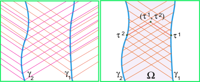
Figure 1: a) Every emitter $\gamma_{i}$ broadcasts his proper time $\tau^{i}$. b) Then, every event in the domain $\Omega$ between both emitters can be distinguished by the times $(\tau^{1},\tau^{2})$.

According to the notions remembered and sketched in the Introduction, such a system of two clocks (emitters) broadcasting their proper times constitutes a relativistic positioning system in the two-dimensional space-time under consideration.

The interior ${\cal R}$ of the above region ${\bar{\cal R}}$ may be a domain (i.e. connected) or, if the clock world lines are allowed to contact or to cut, a union of domains. Anyway, from now on, we shall restrict our study to a sole domain, denoted by $\Omega.$ Thus, according to the allowed situations, we may have $\Omega\equiv{\cal R}$ or $\Omega\subset{\cal R}.$

The domain $\Omega$ constitutes a coordinate domain. Indeed, every event in it can be distinguished by the times $\tau^{1}$ and $\tau^{2}$ received from the emitter clocks. See Fig. 1b. In other words, the past light cone of every event in $\Omega$ cuts the emitter world lines at $\gamma_{1}(\tau^{1})$ and $\gamma_{2}(\tau^{2})$, respectively. Then $(\tau^{1},\tau^{2})$ are the coordinates of the event. We shall refer to them as the emission coordinates $\{\tau^{1},\tau^{2}\}$ of the system.

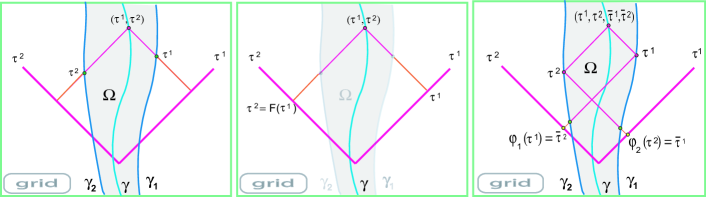
Figure 2: a) Geometric interpretation of the emission coordinates: in the grid $\{\tau^{1}\}\times\{\tau^{2}\}$ the trajectory of a user $\gamma$ that receives the proper times $\{\tau^{1},\tau^{2}\}$ broadcasted by the emitters $\gamma_{1}$, $\gamma_{2}$ is drawn. b) The user positioning data $\{\tau^{1},\tau^{2}\}$ allow the user to know his trajectory in emission coordinates and he can draw it in the grid $\{\tau^{1}\}\times\{\tau^{2}\}$. c) The emitter positioning data $\{\tau^{1},\tau^{2};\bar{\tau}^{1},\bar{\tau}^{2}\}$ allow the user to know the emitter trajectories $\varphi_{1}(\tau^{1})$, $\varphi_{2}(\tau^{2})$ in emission coordinates $\{\tau^{1},\tau^{2}\}$.

On the contrary, all the events outside both world lines that receive the same time $\tau^{1}$ receive also the same time $\tau^{2}$ because both signals are parallel. See Fig. 1a. Thus, these proper times do not distinguish different events on the segment of null geodesic signals in the outside region: the signals $\tau^{1}$ and $\tau^{2}$ do not constitute coordinates for the events in the outside region.

What happens on the clock world lines? The clock world lines are (part of) the boundary of the domain $\Omega,$ so that they are out of it. Nevertheless, there is no ambiguity to associate to their instants, by continuity from $\Omega,$ a pair of proper times: the one of the clock in question and that received from the other clock. We shall refer to these pairs as the emission coordinates of the emitters.

The coordinate lines (coordinate hypersurfaces) of the emission coordinates $\{\tau^{1},\tau^{2}\}$ are null geodesics. Consequently, the emission coordinates are null coordinates. Thus, in emission coordinates the space-time metric depends on the sole metric function $m$ (see Appendix A):

$$ds^{2}=m(\tau^{1},\tau^{2})d\tau^{1}d\tau^{2}$$ (1)

An observer $\gamma,$ traveling throughout the emission coordinate domain $\Omega$ and equipped with a receiver allowing the reading of the received proper times $(\tau^{1},\tau^{2})$ at each point of his trajectory, is called a user of the positioning system.

The essential physical components of the relativistic positioning system are thus:

• Two emitters $\gamma_{1}$, $\gamma_{2}$ broadcasting their proper times $\tau^{1}$, $\tau^{2}$.

• Users $\gamma$ traveling in the domain $\Omega$ and receiving the broadcasted times $\{\tau^{1},\tau^{2}\}.$

Observe that, as a location system (i.e. as a physical realization of a mathematical coordinate system), the above positioning system is generic, free and immediate in the sense specified in the Introduction.

The plane $\{\tau^{1}\}\times\{\tau^{2}\}$ ($\tau^{1},\tau^{2}\in\mathbb{R}$) in which the different data of the positioning system can be transcribed is called the grid of the positioning system. See Fig. 2a. Observe that not all the points of the grid correspond to physical events. Only those limited by the emitter trajectories can be physically detected.

It is worth remarking that any user receiving continuously the emitted times $\{\tau^{1},\tau^{2}\}$ knows his trajectory in the grid. Indeed, from these user positioning data $\{\tau^{1},\tau^{2}\}$ the user trajectory may be drawn in the grid (see Fig. 2b), and its equation $F$,

$$\tau^{2}=F(\tau^{1})\,,$$ (2)

may be extracted from these data.

Let us note that, whatever the user be, these data are insufficient to construct both of the two emitter trajectories.

In order to give to any user the capability of knowing the emitter trajectories in the grid, the positioning system must be endowed with a device allowing every emitter to also broadcast the proper time it is receiving from the other emitter. See Fig. 2c. In other words, the clocks must be allowed to broadcast their emission coordinates. As stated in the Introduction, a positioning system so endowed is called an auto-locating positioning system.

The physical components of an auto-locating positioning system are thus:

• Two emitters $\gamma_{1}$, $\gamma_{2}$ broadcasting their proper times $\tau^{1},$ $\tau^{2}$ and the proper times $\bar{\tau}^{2}$, $\bar{\tau}^{1}$ that they receive each one from the other.

• Users $\gamma$, traveling in $\Omega$ and receiving these four broadcasted times $\{\tau^{1},\tau^{2};\bar{\tau}^{1},\bar{\tau}^{2}\}$.

Any user receiving continuously these emitter positioning data $\{\tau^{1},\tau^{2};\bar{\tau}^{1},\bar{\tau}^{2}\}$ may extract from them not only the equation of his trajectory in the grid, $\tau^{2}=F(\tau^{1}),$ but also the equations of the trajectories of the emitters (see Fig. 2c):

$$\varphi_{1}(\tau^{1})=\bar{\tau}^{2}\,,\qquad\varphi_{2}(\tau^{2})=\bar{\tau}^{1}$$ (3)

Eventually, the positioning system can be endowed with complementary devices. For example, in obtaining the dynamic properties of the system, it is necessary to know the acceleration of the emitters. For this ability:

• The emitters $\gamma_{1}$, $\gamma_{2}$ carry accelerometers and broadcast their acceleration $\alpha_{1}$, $\alpha_{2}$.

• The users $\gamma$, in addition to the emitter positioning data, also receive the emitter accelerations $\{\alpha_{1},\alpha_{2}\}$.

These new elements allow any user (and, in particular, the emitters) to know the acceleration scalar of the emitters:

$$\alpha_{1}=\alpha_{1}(\tau^{1})\,,\qquad\alpha_{2}=\alpha_{2}(\tau^{2})$$ (4)

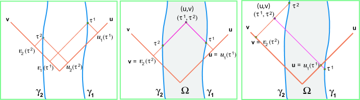
Figure 3: a) Proper time history of two emitters $\gamma_{1}$, $\gamma_{2}$ in a null system $\{\texttt{u},\texttt{v}\}$. b) Geometric interpretation of the coordinate change between emission coordinates $\{\tau^{1},\tau^{2}\}$ and a null system $\{\texttt{u},\texttt{v}\}$. c) Outside the domain $\Omega$, $\{\tau^{1},\tau^{2}\}$ are still null coordinates but not more emission coordinates.

In some cases, it can be useful that the users generate their own data:

• Any user carries a clock that measures his proper time $\tau$.

• Any user carries an accelerometer that measures his acceleration $\alpha$.

The user’s clock allows any user to know his proper time function $\tau(\tau^{1})$ (or $\tau(\tau^{2})$) and, consequently by using (2), to obtain the proper time parametrization of his trajectory:

$$\gamma\equiv\begin{cases}\ \tau^{1}=\tau^{1}(\tau)\\ \ \tau^{2}=\tau^{2}(\tau)\end{cases}$$ (5)

The user’s accelerometer allows any user to know his proper acceleration scalar:

$$\alpha=\alpha(\tau)$$

Thus, a relativistic positioning system may be performed in such a way that any user can obtain a subset of the user data:

$$\{\tau^{1},\tau^{2};\bar{\tau}^{1},\bar{\tau}^{2};\alpha_{1},\alpha_{2};\tau,\alpha\}$$ (6)

It is worth remarking that the pairs of data $\{\tau^{1},\bar{\tau}^{2}\}$ and $\{\tau^{2},\bar{\tau}^{1}\}$ which give the emitter trajectories (3) do not depend on the user that receives them, i.e., every user draws in his user grid the same emitter trajectories. A similar think occurs with the pairs $\{\tau^{1},\alpha_{1}\}$ and $\{\tau^{2},\alpha_{2}\}$ which give the emitter accelerations (4). Thus, among the user data (6) we can distinguish the subsets:

• emitter positioning data $\{\tau^{1},\tau^{2};\bar{\tau}^{1},\bar{\tau}^{2}\}$,

• public data $\{\tau^{1},\tau^{2};\bar{\tau}^{1},\bar{\tau}^{2};\alpha_{1},\alpha_{2}\}$,

• user proper data $\{\tau,\alpha\}$.

The grid of the positioning system plays an important role in practical positioning. Auto-locating systems allow any user to determine the domain $\Omega$ in the grid where the parameters $\{\tau^{1},\tau^{2}\}$ constitute effectively a emission coordinate system, i.e. may be physically detected.

It is to be noted that in a positioning system the emitter clocks are constrained to measure their proper time, but otherwise their time scale (their origin) is completely independent one of the other, that is to say, they are not submitted to any prescribed synchronization. The form of the trajectories of emitters and users in the grid is an invariant of the independently chosen time scales, only their position in the grid translates with them.

III Construction of the emission coordinates

In a generic two-dimensional space-time let $\{\texttt{u},\texttt{v}\}$ be an arbitrary null coordinate system, i.e., a coordinate system where the metric interval can be written (see appendix A):

$$ds^{2}=\texttt{m}(\texttt{u},\texttt{v})\,d\texttt{u}\,d\texttt{v}$$

Let us assume the proper time history of two emitters to be known in this coordinate system (see Fig. 3a):

$$\gamma_{1}\equiv\begin{cases}\texttt{u}=u_{1}(\tau^{1})\\ \texttt{v}=v_{1}(\tau^{1})\end{cases}\qquad\gamma_{2}\equiv\begin{cases}\texttt{u}=u_{2}(\tau^{2})\\ \texttt{v}=v_{2}(\tau^{2})\end{cases}$$ (7)

We can introduce the proper times as coordinates $\{\tau^{1},\tau^{2}\}$ by defining the change to the null system $\{\texttt{u},\texttt{v}\}$ given by (see Fig. 3b):

$$\begin{array}[]{l}\texttt{u}=u_{1}(\tau^{1})\\ \texttt{v}=v_{2}(\tau^{2})\end{array}\qquad\quad\begin{array}[]{l}\tau^{1}=u_{1}^{-1}(\texttt{u})=\tau^{1}(\texttt{u})\\ \tau^{2}=v_{2}^{-1}(\texttt{v})=\tau^{2}(\texttt{v})\end{array}$$ (8)

In terms of the coordinates $\{\texttt{u},\texttt{v}\}$, the region $\Omega$ where the new coordinates $\{\tau^{1},\tau^{2}\}$ can be considered emitted times is (see Fig. 3b):

$$\Omega\equiv\big{\{}(\texttt{u},\texttt{v})\ |\ F_{2}^{-1}(\texttt{v})\leq\texttt{u}\,,\quad F_{1}(\texttt{u})\leq\texttt{v}\big{\}}$$

where $F_{i}$ are the emitter trajectory functions:

$$\texttt{v}=F_{i}(\texttt{u})\,,\qquad F_{i}=v_{i}\circ u_{i}^{-1}$$ (9)

Thus, relations (8) define emission coordinates in the emission coordinate domain $\Omega$.

In the region outside $\Omega$ the change (8) also determines null coordinates which are an extension of the emission coordinates. But in this region the coordinates are not physical, i.e. are not the emitted proper times of the emitters $\gamma_{1}$, $\gamma_{2}$ . See Fig. 3c. Note that there are several null coordinate systems that can be associated with a unique observer or with two observers by considering their advanced or retarded signals. But here we are limited to emission coordinates: those generated by a positioning system and thus by retarded signals.

In emission coordinates, the emitter trajectories take the expression (see Fig. 4):

$$\gamma_{1}\equiv\begin{cases}\tau^{1}=\tau^{1}\\ \tau^{2}=\varphi_{1}(\tau^{1})\end{cases}\qquad\gamma_{2}\equiv\begin{cases}\tau^{1}=\varphi_{2}(\tau^{2})\\ \tau^{2}=\tau^{2}\end{cases}$$ (10)

where, from (7) and (8), the functions $\varphi_{i}$ giving the emitter trajectories are given by:

$$\varphi_{1}=v_{2}^{-1}\circ v_{1}\,,\qquad\varphi_{2}=u_{1}^{-1}\circ u_{2}$$ (11)

The principal observers associated with an arbitrary null system are those whose proper time coincides with one of the two null coordinates (see appendix C). The expression (10) shows that:  
The two emitters are particular principal observers of the emission coordinate system that they define.

Finally, if we know the metric function $\texttt{m}(\texttt{u},\texttt{v})$ in null coordinates $\{\texttt{u},\texttt{v}\}$, we can obtain the metric interval in emission coordinates $\{\tau^{1},\tau^{2}\}$ by using the change (8):

$$\begin{array}[]{c}ds^{2}=m(\tau^{1},\tau^{2})d\tau^{1}d\tau^{2}\\[11.38109pt] m(\tau^{1},\tau^{2})=\texttt{m}(u_{1}(\tau^{1}),v_{2}(\tau^{2}))u_{1}^{\prime}(\tau^{1})v_{2}^{\prime}(\tau^{2})\end{array}$$ (12)

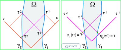
Figure 4: Emitter trajectories in a coordinate diagram $\{\texttt{u},\texttt{v}\}$ and in the grid $\{\tau^{1},\tau^{2}\}$.

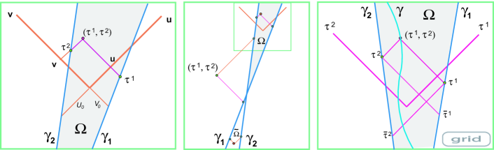
Figure 5: a) Proper time parametrization of geodesic emitters $\gamma_{1}$, $\gamma_{2}$ and associated emission coordinates $\{\tau^{1},\tau^{2}\}$. b) The coordinates $\{\tau^{1},\tau^{2}\}$ defined in (14) can be extended, but outside of $\Omega$ they are not emission coordinates. c) Trajectories of geodesic emitters in the grid, where the ‘initial’ inertial information does not appear.

IV Positioning with inertial emitters

In this section we consider the simple example of a positioning system defined by two inertial emitters $\gamma_{1}$, $\gamma_{2}$ in flat space-time.

In inertial null coordinates $\{\texttt{u},\texttt{v}\}$ the trajectory of the emitters are (see Fig. 5a):

$$\begin{array}[]{lcl}\gamma_{1}&:&\qquad\texttt{v}=\displaystyle\frac{1}{\lambda_{1}^{2}}\texttt{u}+v_{0}\\[8.53581pt] \gamma_{2}&:&\qquad\texttt{v}=\displaystyle\frac{1}{\lambda_{2}^{2}}(\texttt{u}-u_{0})\end{array}$$

where $\lambda_{1}$, $\lambda_{2}$ are the shifts of the emitters with respect to the inertial system. We could choose these inertial coordinates so that one emitter be at rest. The constants $u_{0}$ and $v_{0}$ can also be arbitrarily chosen depending on the inertial origin. But, for the moment, we will consider that they take arbitrary values. In Fig. 5 we have take $u_{0}<0$, $v_{0}<0$ and $1\leq\lambda_{2}\leq\lambda_{1}$.

The origin of the emitter proper times can be taken such that the proper time history of the emitters be:

$$\gamma_{1}\equiv\begin{cases}\,\texttt{u}=\lambda_{1}\tau^{1}\\[2.84526pt] \,\texttt{v}=\displaystyle\frac{1}{\lambda_{1}}\tau^{1}+v_{0}\end{cases}\ \gamma_{2}\equiv\begin{cases}\,\texttt{u}=\lambda_{2}\tau^{2}+u_{0}\\[2.84526pt] \,\texttt{v}=\displaystyle\frac{1}{\lambda_{2}}\tau^{2}\end{cases}$$ (13)

Then, taking into account the construction presented in previous section, the coordinate transformation from the inertial coordinate system $\{\texttt{u},\texttt{v}\}$ to the emission coordinate system $\{\tau^{1},\tau^{2}\}$ is given by (see Fig. 5a):

$$\begin{array}[]{lll}\texttt{u}=u_{1}(\tau^{1})=\lambda_{1}\tau^{1}&&\tau^{1}=\displaystyle\frac{1}{\lambda_{1}}\,\texttt{u}\\[5.69054pt] \texttt{v}=v_{2}(\tau^{2})=\displaystyle\frac{1}{\lambda_{2}}\tau^{2}&&\tau^{2}=\lambda_{2}\texttt{v}\end{array}$$ (14)

From this transformation, the metric tensor in emission coordinates $\{\tau^{1},\tau^{2}\}$ can be obtained. Indeed, from (12) we have:

$$m(\tau^{1},\tau^{2})=u_{1}^{\prime}(\tau^{1})v_{2}^{\prime}(\tau^{2})=\frac{\lambda_{1}}{\lambda_{2}}$$

Thus, the metric function is constant and equals the relative shift between both emitters:

$$ds^{2}=\lambda\,d\tau^{1}d\tau^{2}\,,\qquad\lambda\equiv\frac{\lambda_{1}}{\lambda_{2}}$$

It is worth pointing out that the coordinates $\{\tau^{1},\tau^{2}\}$ defined in (14) can be extended throughout the whole space-time (see Fig. 5b), but that outside the domain $\Omega$ they are not emission coordinates. Nor are they in the domain $\tilde{\Omega}$ in Fig. 5b, where they are “advanced-advanced” coordinates.

Of course, in this domain $\tilde{\Omega}$ the emitters $\gamma_{1}$, $\gamma_{2}$ also define emission coordinates, but they are not given by (14). In this case we must interchange the role of both emitters. Then, in $\tilde{\Omega}$ the emission coordinates $\{\tilde{\tau}^{1},\tilde{\tau}^{2}\}$ are given by:

$$\begin{array}[]{l}\texttt{u}=\lambda_{2}\tilde{\tau}^{1}+u_{0}\\[2.84526pt] \texttt{v}=\displaystyle\frac{1}{\lambda_{1}}\tilde{\tau}^{2}+v_{0}\end{array}$$ (15)

and the metric tensor is now:

$$ds^{2}=\frac{1}{\lambda}\,d\tilde{\tau}^{1}d\tilde{\tau}^{2}\,,\qquad\lambda\equiv\frac{\lambda_{1}}{\lambda_{2}}$$

The coordinates $\{\tilde{\tau}^{1},\tilde{\tau}^{2}\}$ can also be extended to the whole space-time, but only on the domain $\tilde{\Omega}$ are emission coordinates.

Note that the extensions of the emission coordinates (14) and (15) are different everywhere when $\lambda\not=1$. When the emitters are at rest with each other ($\lambda=1$), both extensions coincide (up to an origin change) and they define inertial coordinates.

Let us return now to our domain $\Omega$ where the emission coordinates are given by (14). In these coordinates $\{\tau^{1},\tau^{2}\}$, the emitter trajectories are (see Fig. 5c):

$$\gamma_{1}\equiv\begin{cases}\tau^{1}=\tau^{1}\\ \tau^{2}=\varphi_{1}(\tau^{1})\equiv\displaystyle\frac{1}{\lambda}\tau^{1}+\tau^{2}_{0}\end{cases}$$ (16)

$$\gamma_{2}\equiv\begin{cases}\tau^{1}=\varphi_{2}(\tau^{2})\equiv\displaystyle\frac{1}{\lambda}\tau^{2}+\tau^{1}_{0}\\ \tau^{2}=\tau^{2}\end{cases}$$ (17)

Observe that these emitter trajectories in the grid have lost the ‘initial’ inertial information of the null coordinate system $\{\texttt{u},\texttt{v}\}$. Indeed, only the shift $\lambda$ between the emitters appears (and not the relative shift $\lambda_{i}$ of each emitter with respect to the inertial system), and the grid origin depends exclusively on the choice of origin of the emitter times (not on the inertial coordinate origin). See Fig. 5c for the case $\lambda\not=0$; for emitters at rest with each other the emitter trajectories become parallel.

What information can a user obtain from the public data? Evidently $\{\tau^{1},\tau^{2}\}$ place the user on the grid, and $\{\tau^{1},\tau^{2},\bar{\tau}^{1},\bar{\tau}^{2}\}$, $\bar{\tau}^{i}=\varphi_{j}(\tau^{j})$, make the same for the emitters.

On the other hand, we can observe in (16), (17) that the metric function $m(\tau^{1},\tau^{2})=\lambda$ can be obtained from the emitter positioning data $\{\tau^{1}_{P},\tau^{2}_{P};\bar{\tau}^{1}_{P},\bar{\tau}^{2}_{P}\}$ and $\{\tau^{1}_{Q},\tau^{2}_{Q};\bar{\tau}^{1}_{Q},\bar{\tau}^{2}_{Q}\}$ at two events $P$ and $Q$. Thus we have:

Proposition 1

In terms of the emitter positioning data $\{\tau^{1},\tau^{2};\bar{\tau}^{1},\bar{\tau}^{2}\}$, the space-time metric is given by

$$ds^{2}=\sqrt{\frac{\Delta\tau^{1}\Delta\tau^{2}}{\Delta\bar{\tau}^{1}\Delta\bar{\tau}^{2}}}\,d\tau^{1}d\tau^{2}$$ (18)

where $\Delta\tau^{i},$ $\Delta\bar{\tau}^{i}$ stand for the differences of values at two events.

Although simple, this statement is very important because it shows that, if the emitters are geodesic, the sole public quantities $\{\tau^{1},\tau^{2};\bar{\tau}^{1},\bar{\tau}^{2}\}$ received by any user allow him to know the space-time metric everywhere.

Observe that when both emitter clocks are synchronized such that they indicate the instant zero at the virtual cut event ($\tau^{1}_{c}=\tau^{2}_{c}=0$), the user only needs to know the emitter positioning data at one event and the space-time metric reduces then to:

$$ds^{2}=\sqrt{\frac{\tau^{1}\tau^{2}}{\bar{\tau}^{1}\bar{\tau}^{2}}}\,d\tau^{1}d\tau^{2}$$ (19)

Note that even if we know that the clocks are geodesic, (19) cannot be applied unless the clocks be synchronized in the way above mentioned and the users know this fact, meanwhile (18) is valid whatever be the synchronization of the geodesic clocks. Furthermore, the trajectories of the clocks in the grid being then known and the metric being given by (18), a simple computation allows to know the precise synchronization of the clocks (i.e. the values $\tau^{1}_{c}$ and $\tau^{2}_{c}$ of the virtual cut event).

The geodesic character of the clocks may be an a priori information forming part of the dynamical characteristics of the clocks and the foreseen control of the system, or may be also a real time information if clocks and users are endowed with devices allowing the users to know the emitter accelerations $\{\alpha_{1},\alpha_{2}\}$. In any case, the user information of the geodesic character of the clocks by any of these two methods is generically necessary, because emitter trajectories that are straight lines in the user grid are not necessarily geodesic trajectories in the space-time cfm .

V Gravimetry and positioning

We already know that, whatever be the curvature of the two-dimensional space-time, the emitter positioning data

$$\{\tau^{1},\tau^{2};\bar{\tau}^{1},\bar{\tau}^{2}\}$$ (20)

determine, on one hand, the user trajectory

$$\tau^{2}=F(\tau^{1})$$

and, on the other hand, the emitter trajectories $\varphi_{i}$,

$$\bar{\tau}^{2}=\varphi_{1}(\tau^{1})\,,\qquad\bar{\tau}^{1}=\varphi_{2}(\tau^{2})$$

But, what about the metric interval when the user has no information about the gravitational field? In other words, what gravimetry can a user do from the data offered by a positioning system?

From the sole emitter positioning data (20) and denoting by a dot the derivative with respect to the corresponding proper time, one has:

Proposition 2

The emitter positioning data $\{\tau^{1},\tau^{2};\bar{\tau}^{1},\bar{\tau}^{2}\}$ determine the space-time metric function along the emitter trajectories, namely:

$$m(\tau^{1},\varphi_{1}(\tau^{1}))=\frac{1}{\dot{\varphi}_{1}(\tau^{1})}$$ (21)

$$m(\varphi_{2}(\tau^{2}),\tau^{2})=\frac{1}{\dot{\varphi}_{2}(\tau^{2})}$$ (22)

This result follows from the fact that emitters are also principal observers for the emission coordinates and the kinematic expression (38) for these observers.

If in addition of the emitter positioning data (20) the user knows the emitter accelerations $\{\alpha_{1},\alpha_{2}\}$, and thus the acceleration scalars $\alpha_{1}(\tau^{1})$, $\alpha_{2}(\tau^{2})$, one has also the following metric information:

Proposition 3

The public data $\{\tau^{1},\tau^{2};\bar{\tau}^{1},\bar{\tau}^{2};\alpha_{1},\alpha_{2}\}$ determine the gradient of the space-time metric function along the emitter trajectories, namely:

$$\begin{array}[]{l}(\ln m),_{1}(\tau^{1},\varphi_{1}(\tau^{1}))=\alpha_{1}(\tau^{1})\\[5.69054pt] \displaystyle(\ln m),_{2}(\tau^{1},\varphi_{1}(\tau^{1}))=\frac{-1}{\dot{\varphi}_{1}(\tau^{1})}\left[\alpha_{1}(\tau^{1})+\frac{\ddot{\varphi}_{1}(\tau^{1})}{\dot{\varphi}_{1}(\tau^{1})}\right]\end{array}$$ (23)

$$\begin{array}[]{l}\displaystyle(\ln m),_{1}(\tau^{2},\varphi_{2}(\tau^{2}))=\frac{1}{\dot{\varphi}_{2}(\tau^{2})}\left[\alpha_{2}(\tau^{2})-\frac{\ddot{\varphi}_{2}(\tau^{2})}{\dot{\varphi}_{2}(\tau^{2})}\right]\\[17.07164pt] (\ln m),_{2}(\varphi_{2}(\tau^{2}),\tau^{2})=-\alpha_{2}(\tau^{2})\end{array}$$ (24)

This result follows from expression (40) of the scalar acceleration of the principal observers and the fact that once the metric function $m(\tau^{1},\tau^{2})$ is known on a trajectory, the knowledge of its gradient needs only of one transverse partial derivative.

Alternatively, even when the positioning system is not auto-locating, i.e., it broadcast only the proper times $\{\tau^{1},\tau^{2}\}$, if in addition the user also knows the proper user data $\{\tau,\alpha\}$, he may obtain gravimetric information along his trajectory. From his proper time $\tau$ measured by his clock, he can know his proper time function, say $\tau=\tau(\tau^{1})$, by comparing $\tau$ with the proper time $\tau^{1}$ received from the emitter $\gamma_{1}$; consequently he can obtain his parameterized proper time trajectory:

$$\begin{array}[]{l}\tau^{1}=\tau^{1}(\tau)\\ \tau^{2}=\tau^{2}(\tau)\end{array}$$

From his accelerometer he can obtain his acceleration scalar $\alpha(\tau)$. Then, the user may have the following gravimetry information:

Proposition 4

The public-user data $\{\tau^{1},\tau^{2};\tau,\alpha\}$ determine the space-time metric function and its gradient on the user trajectory, namely:

$$m(\tau^{1}(\tau),\tau^{2}(\tau))=\frac{1}{\dot{\tau}^{1}(\tau)\dot{\tau}^{2}(\tau)}$$ (25)

$$\begin{array}[]{l}\displaystyle(\ln m),_{1}(\tau^{1}(\tau),\tau^{2}(\tau))=\frac{1}{\dot{\tau}^{1}(\tau)}\left[\alpha(\tau)-\frac{\ddot{\tau}^{1}(\tau)}{\dot{\tau}^{1}(\tau)}\right]\\[8.53581pt] \displaystyle(\ln m),_{2}(\tau^{1}(\tau),\tau^{2}(\tau))=-\frac{1}{\dot{\tau}^{2}(\tau)}\left[\alpha(\tau)+\frac{\ddot{\tau}^{2}(\tau)}{\dot{\tau}^{2}(\tau)}\right]\end{array}$$ (26)

This result follows from expressions (32) and (34) on kinematics in null coordinates.

As an example of these kinds of information, let us consider a user, with no previous information on the gravitational field, and receiving the following specific public data $\{\tau^{1},\tau^{2};\bar{\tau}^{1},\bar{\tau}^{2};\alpha_{1},\alpha_{2}\}$, namely emitter positioning data $\{\tau^{1},\tau^{2};\bar{\tau}^{1},\bar{\tau}^{2}\}$ showing a particular linear relation between the $\bar{\tau}$’s and the $\tau$’s:

$$\begin{array}[]{l}\bar{\tau}^{2}=\varphi_{1}(\tau^{1})\equiv\displaystyle\frac{1}{\lambda}\tau^{1}+\tau^{2}_{0}\\ \vspace{-2mm}\\ \bar{\tau}^{1}=\varphi_{2}(\tau^{2})\equiv\displaystyle\frac{1}{\lambda}\tau^{2}+\tau^{1}_{0}\end{array}$$ (27)

with $\lambda>1$ and vanishing public data $\{\alpha_{1},\alpha_{2}\}$:

$$\alpha_{1}(\tau^{1})=0\,,\quad\alpha_{2}(\tau^{2})=0$$ (28)

Then, proposition 2 gives the following metric function along the emitter trajectories:

$$m(\tau^{1})=\lambda\ ,\qquad m(\tau^{2})=\lambda\,,$$

and proposition 3 implies that the gradient of the metric function vanishes along the emitter trajectories:

$$m,_{1}(\tau^{1})=m,_{2}(\tau^{1})=0\,,\qquad m,_{1}(\tau^{2})=m,_{2}(\tau^{2})=0$$

Let us note that the above specific public data (27), because of their complementary slopes, coincide with those generated by the positioning system defined by two geodesic emitters in flat space-time, as considered in section IV (see expressions (16), (17), and Fig. 5c). Nevertheless, it is to be remarked that the same specific emitter positioning data $\{\tau^{1},\tau^{2};\bar{\tau}^{1},\bar{\tau}^{2}\}$ verifying (27) could be obtained from non geodesic emitters in flat space-time as well as by geodesic or not geodesic emitters in a non flat space-time. Also, the same specific public data $\{\tau^{1},\tau^{2};\bar{\tau}^{1},\bar{\tau}^{2};\alpha_{1},\alpha_{2}\}$ verifying (27) and (28) could be obtained from geodesic emitters in a non flat space-time. This point will be analyzed in detail elsewhere cfm .

VI Discussion and work in progress

In this work we have explained the basic features of relativistic positioning systems in a two-dimensional space-time (section II) and have obtained the analytic expression of the emission coordinates associated with such a system (section III). In order to a better understanding of these systems we have developed an example in detail: the positioning system defined in flat space-time by geodesic emitters, showing the striking result that the emitted and transmitted times allow a complete determination of the metric in emission coordinates (section IV). Finally, we have shown that the data that a user obtains from the positioning system in arbitrary space-times determine the gravitational field and its gradient along the emitters and user world lines (section V).

It is worth remarking that the extension to the four-dimensional case of the two-dimensional methods used here needs of additional information. In particular, the information of the angles between pairs of the arrival signals broadcasted by the clocks could help in the obtention of the gravitational field along the trajectory of the user coll-pozo ; pozo .

Nevertheless, the two-dimensional approach presented here helps strongly to the understanding of how positioning systems work and what is the physical role of their basic elements. We have used explicit diagrams that improve the qualitative comprehension of these systems and we have obtained simple analytic results. These advantages encourage in putting and solving new two-dimensional problems, many of them appearing in a natural way from the results presented in this work.

Elsewhere cfm we consider positioning systems in flat metric other than that defined by geodesic emitters. Our first results on this matter show interesting behaviors. For example, trajectories of uniformly accelerated emitters are parallel straight lines in the grid, as also happens with the trajectories of some other emitters with more complicated acceleration laws.

Moreover, as a first contact to understand the behavior of relativistic positioning systems in a non flat gravitational field, we study positioning systems defined in the Schwarzschild plane by two stationary emitters cfm .

The study of these two cases of uniformly accelerated emitters brings to light an interesting situation: the emitter positioning data of both systems lead to an identical public grid. How a user can distinguish both systems? In cfm we analyze this question and show that the full set of the user data determine the Schwarzschild mass. This simple two-dimensional example suggests that the relativistic positioning systems could be useful in gravimetry for reasonable parameterized models of the gravitational field.

This gravimetry case is only a particular situation of the general gravimetry problem in Relativity where user data are the unique information that a user has. We have shown here that these data allow the user to obtain the metric function and its gradient on some trajectories. This information on the gravitational field can be increased introducing ‘secondary’ emitters, that broadcast the information they receive from the system, allowing any user to know the metric function and its gradient on these additional trajectories.

Some circumstances can lead us to take the point of view where the user knows the space-time in which he is immersed (Minkowski, Schwarzschild,…) and he wants to obtain, from the user data, information on his local unities of time and distance, his acceleration, the metric expression in the emission coordinates, and his trajectory and emitters trajectories in a characteristic coordinate system of the given space-time (inertial in flat metric, stationary coordinates in Schwarzschild o other stationary metric,…).

We undertake this problem for the flat case in cfm , where we analyze the minimum set of data that determine all this system and user information. A striking result is that the user data are not independent quantities: if we know the emitter positioning data, then the accelerations of the emitters and of the user along their trajectories are determined by the sole knowledge of one acceleration during only an echo-causal interval between the emitter trajectories.

Appendix A Two-dimensional metrics in null coordinates

Here several simple and general results about two-dimensional metrics are summarized and some usual relativistic questions are developed by using the so called null coordinates.

In a flat two-dimensional space-time, with every inertial coordinate system $\{t,x\}$ we can associate inertial null coordinates $\{\texttt{u},\texttt{v}\}$:

$$\begin{array}[]{ll}\texttt{u}=t+x&\qquad\qquad t=\frac{1}{2}(\texttt{u}+\texttt{v})\\[2.84526pt] \texttt{v}=t-x&\qquad\qquad x=\frac{1}{2}(\texttt{u}-\texttt{v})\end{array}$$

In coordinates $\{\texttt{u},\texttt{v}\}$, the metric tensor takes the form:

$$ds^{2}=dt^{2}-dx^{2}=d\texttt{u}\,d\texttt{v}$$

A boost between two inertial systems $\{t,x\}$, $\{\bar{t},\bar{x}\}$ with a relative velocity $\beta=\tanh\psi$ takes a simple expression in inertial null coordinates $\{\texttt{u},\texttt{v}\}$, $\{\bar{\texttt{u}},\bar{\texttt{v}\}}$:

$$\begin{array}[]{l}\bar{\texttt{u}}=e^{\psi}\texttt{u}\\[2.84526pt] \bar{\texttt{v}}=e^{-\psi}\texttt{v}\end{array}$$ (29)

Let us note that the factor

$$s=e^{\psi}=\sqrt{\frac{1+\beta}{1-\beta}}=1+z$$

is the shift parameter between both inertial systems.

An important result in two-dimensional Riemannian geometry states that every two-dimensional metric is (locally) conformally flat. In the Lorentzian case, starting from the inertial systems associated with the flat metric conformal to the given space-time metric, we see that null coordinates $\{\texttt{u},\texttt{v}\}$ exist such that

$$ds^{2}=m(\texttt{u},\texttt{v})\,d\texttt{u}\,d\texttt{v}$$

In a two-dimensional geometry $g$ the scalar curvature $R(g)$ is the unique strict component of the Riemann tensor. In terms of the conformal factor $m$ the scalar curvature is:

$$R(g)=\frac{1}{m}\Delta\ln m=\Delta_{g}\ln m\,,\qquad g=m\eta$$

where $\Delta$ is the Laplacian operator for the flat metric $\eta$. From here, it follows that a two-dimensional metric is flat iff the logarithm of the conformal factor is an harmonic function.

Consequently: a two-dimensional Lorentzian metric is flat iff the conformal factor factorizes in null coordinates, that is to say:

$$m(\texttt{u},\texttt{v})=U(\texttt{u})V(\texttt{v})$$

In this flat case, the change of coordinates from a generic null system $\{\texttt{u},\texttt{v}\}$ to an inertial one $\{\bar{\texttt{u}},\bar{\texttt{v}}\}$ is given by

$$\begin{array}[]{l}\bar{\texttt{u}}=\bar{\texttt{u}}(\texttt{u})\\[2.84526pt] \bar{\texttt{v}}=\bar{\texttt{v}}(\texttt{v})\end{array}$$ (30)

where $\quad\bar{\texttt{u}}^{\prime}(\texttt{u})=U(\texttt{u})\,,\quad\bar{\texttt{v}}^{\prime}(\texttt{v})=V(\texttt{v})$.

For a non (necessarily) flat metric, the change (30) gives the internal transformation between null coordinates, the metric tensor changing as:

$$ds^{2}=m(\texttt{u},\texttt{v})\,d\texttt{u}\,d\texttt{v}=\bar{m}(\bar{\texttt{u}},\bar{\texttt{v}})\,d\bar{\texttt{u}}\,d\bar{\texttt{v}}$$

$$m(\texttt{u},\texttt{v})=\bar{m}(\bar{\texttt{u}}(\texttt{u}),\bar{\texttt{v}}(\texttt{v}))\,\bar{\texttt{u}}^{\prime}(\texttt{u})\,\bar{\texttt{v}}^{\prime}(\texttt{v})$$

What does this internal transformation (30) mean from a geometric point of view? Any Lorentzian two-dimensional metric defines in the corresponding space-time two (geodesic) null congruences of curves or, what is two-dimensionally equivalent, two families of null hypersurfaces. The space-time functions that have one of these families as level hypersurfaces are the null coordinate functions. Evidently, these functions are defined up to a change given by (30). So, the coordinate lines (or the coordinate hypersurfaces) are invariant under this internal transformation but they are parameterized in a different way in every null coordinate system.

Appendix B Two-dimensional kinematics in null coordinates

Now we will consider some basic kinematic results expressed in a given null coordinate system $\{\texttt{u},\texttt{v}\}$. In terms of his proper time $\tau$, the trajectory of an observer $\gamma$ is:

$$\begin{array}[]{l}\texttt{u}=u(\tau)\\[2.84526pt] \texttt{v}=v(\tau)\end{array}$$ (31)

and its tangent vector:

$$T(\tau)=(T^{{\mbox{\scriptsize u}}},T^{{\mbox{\scriptsize v}}})=(\dot{u}(\tau),\dot{v}(\tau))$$

where a dot means derivative with respect proper time. The unit condition for $T$ connects the metric function $m(\texttt{u},\texttt{v})$ with the observer trajectory (31):

$$m(u(\tau),v(\tau))=\frac{1}{\dot{u}(\tau)\dot{v}(\tau)}$$ (32)

This relation plays an important role in two-dimensional positioning and states that: when the unit tangent vector of an observer is known in terms of his proper time, the metric on the trajectory of this observer is also known.

The proper time parameterized trajectory (31) tantamounts to a (geometric) trajectory $\texttt{v}=F(\texttt{u})$ and a proper time function $\tau=\tau(\texttt{u})$ restricted by the unit condition. From one of the expressions (31) we can obtain the proper time of the observer $\gamma$, say:

$$\tau=\tau(\texttt{u})=u^{-1}(\texttt{u})$$

Then the trajectory is given by:

$$\texttt{v}=F(\texttt{u})=v(\tau(\texttt{u}))\,,$$

and the unit condition (32) can be written:

$$[\tau^{\prime}(\texttt{u})]^{2}=m(\texttt{u},F(\texttt{u}))F^{\prime}(\texttt{u})$$ (33)

From expression (33) it follows that, when a proper time relation $\tau=\tau(\texttt{u})$ is previously given, on any fixed event a trajectory passes which admits this $\tau$ as proper time. This is because to fix the event $(\texttt{u}_{0},\texttt{v}_{0})$ is to fix an initial condition for $F({\rm u})$, namely $\texttt{v}_{0}=F(\texttt{u}_{0})$. In other words, there always exists a congruence of users having a prescribed proper time function.

The acceleration of the observer (31) in null coordinates $\{\texttt{u},\texttt{v}\}$ takes the expression:

$$a(\tau)=(a^{\mbox{\scriptsize u}},a^{\mbox{\scriptsize v}})=\left(\ddot{u}+(\ln m),_{\mbox{\scriptsize u}}\dot{u}^{2},\,\ddot{v}+(\ln m),_{\mbox{\scriptsize v}}\dot{v}^{2}\right)$$

and the acceleration scalar $\alpha(\tau)\equiv\pm\sqrt{-a^{2}(\tau)}$ is:

$$\alpha(\tau)=\frac{\ddot{u}}{\dot{u}}+(\ln m),_{{\mbox{\scriptsize u}}}\dot{u}=-\frac{\ddot{v}}{\dot{v}}-(\ln m),_{{\mbox{\scriptsize v}}}\dot{v}$$ (34)

The dynamic equation, i.e. the equation for the world lines with a known acceleration $\alpha$, and consequently the geodesic equation (when $\alpha=0$), can be written as two coupled equations for the proper time functions $\,u(\tau)$ and $v(\tau)$:

$$\begin{array}[]{c}\displaystyle\frac{\ddot{u}}{\dot{u}}+(\ln m),_{u}\dot{u}=\alpha(\tau)\\ \vspace{-4mm}\hfil\\ m\dot{u}\dot{v}=1\end{array}$$ (35)

In (35) $m(\texttt{u},\texttt{v})$ is known, and $m$ stands for $m(u(\tau),v(\tau))$; therefore, it is a coupled system.

Appendix C Principal observers for two-dimensional null coordinates

In appendix B we have seen that every proper time function defines a congruence of observers. To every null coordinate system $\{\texttt{u},\texttt{v}\}$ two special congruences of observers exist, called principal observers of the system: those whose proper time coincides with one of the two null coordinates. Thus, we have the u-principal observers:

$$\begin{array}[]{l}{\rm u}=\tau\\ {\rm v}=\varphi_{{\rm u}}({\rm u})\end{array}$$ (36)

and the v-principal observers:

$$\begin{array}[]{l}{\rm u}=\varphi_{{\rm v}}({\rm v})\\ {\rm v}=\tau\end{array}$$ (37)

The tangent vectors to the principal observers are:

$$T_{\rm u}=(1,\dot{\varphi}_{\rm u})\,,\qquad T_{\rm v}=(\dot{\varphi}_{\rm v},1)\,,$$

and the unit condition takes the form:

$$m(\texttt{u},\varphi_{\rm u}({\mbox{u}}))=\frac{1}{\dot{\varphi}_{\rm u}({\rm u})}\,,\quad m(\varphi_{\rm v}(\texttt{v}),\texttt{v})=\frac{1}{\dot{\varphi}_{\rm v}(\texttt{v})}$$ (38)

For the principal observers the acceleration becomes:

$$\begin{array}[]{l}a_{\rm u}({\mbox{u}})=\left((\ln m),_{\rm u}\,,\,\ddot{\varphi}_{\rm u}+(\ln m),_{\rm v}\dot{\varphi}_{\rm u}^{2}\right)\\[5.69054pt] a_{\rm v}(\texttt{v})=\left(\ddot{\varphi}_{\rm v}+(\ln m),_{\rm u}\dot{\varphi}_{\rm v}^{2}\,,\,(\ln m),_{\rm v}\right)\end{array}$$ (39)

And the acceleration scalar is:

$$\begin{array}[]{lcl}\alpha_{\rm u}(\texttt{u})&=&(\ln m),_{\rm u}(\texttt{u},\varphi_{\rm u}({\mbox{u}}))=\\[2.84526pt] &=&\displaystyle-\frac{\ddot{\varphi}_{\rm u}(\texttt{u})}{\dot{\varphi}_{\rm u}(\texttt{u})}-\dot{\varphi}_{\rm u}(\texttt{u})(\ln m),_{\rm v}(\texttt{u},\varphi_{\rm u}({\mbox{u}}))\\[11.38109pt] \alpha_{\rm v}(\texttt{v})&=&-(\ln m),_{\rm v}(\varphi_{\rm v}(\texttt{v}),\texttt{v})=\\[2.84526pt] &=&\displaystyle\frac{\ddot{\varphi}_{\rm v}(\texttt{v})}{\dot{\varphi}_{\rm v}(\texttt{v})}+\dot{\varphi}_{\rm v}(\texttt{v})(\ln m),_{\rm u}(\varphi_{\rm v}(\texttt{v}),\texttt{v})\end{array}$$ (40)

References

- (1) B. Coll, in Proceedings Journées Systèmes de Référence, Bucarest, 2002, edited by N. Capitaine et al. (Observatoire de Paris, Paris, France, 2003). See also gr-qc/0306043.
- (2) B. Coll and A. Tarantola, in Proceedings Journées Systèmes de Référence, St. Petersburg, 2003, edited by A. Finkelstein et al. (Institute of Applied Astronomy of Russian Academy od Science, St. Petesburg, Russia, 2004). See also http//coll.cc.
- (3) B. Coll, in Proceedings of the XXVIII Spanish Relativity Meeting ERE-2005 on A Century of Relativity Physics, AIP Conf. Proc. (AIP, New York, 2006). See also gr-qc/0601110.
- (4) B. Coll, in Proceedings of the XXIII Spanish Relativity Meeting ERE-2000 on Reference Frames and Gravitomagnetism (World Scientific, Singapore, 2000), p. 53. See also http://coll.cc.
- (5) B. Coll, and J.M. Pozo, Phys. Rev. D (to be published).
- (6) J.M. Pozo, in Proceedings Journées Systèmes de Référence, Warsaw, 2005. (to be published). See also gr-qc/0601125.
- (7) B. Coll and J.A. Morales, Intern. Jour. of Theor. Phys. 31, 1045 (1992).
- (8) J.A. Morales, in Proceedings of the XXVIII Spanish Relativity Meeting ERE-2005 on A Century of Relativity Physics, AIP Conf. Proc. (AIP, New York, 2006). See also gr-qc/0601138.
- (9) E.C. Zeeman, Jour. of Math. Phys. 5, 490 (1964).
- (10) G. H. Derrick, Jour. of Math. Phys. 22, 2896 (1981).
- (11) B. Coll, and J.A. Morales, Jour. of Math. Phys. 32, 2450 (1991).
- (12) B. Coll, in Trobades Científiques de la Mediterrània: Actes dels “ERE 85”, Pub. Servei de Publicacions de l’ETSEIB, Barcelona, p. 29-38, 1985. See also http://coll.cc for an English version.
- (13) D. Finkelstein, and J. Michael Gibbs, Intern. Jour. of Theor. Phys. 32, 1801 (1993); D. Finkelstein, Quantum Relativity, (Springer-Verlag, Berlin, 1994).
- (14) T.B. Bahder, Am. J. Phys. 69, 315 (2001).
- (15) C. Rovelli, Phys. Rev. D 65, 044017 (2002).
- (16) J Blagojević., J. Garecki, F. Hehl, and Yu. Obukhov, Phys. Rev. D 65, 044018-1 (2002).
- (17) J.J. Ferrando, in Proceedings of the XXVIII Spanish Relativity Meeting ERE-2005 on A Century of Relativity Physics, AIP Conf. Proc. (AIP, New York, 2006). See also gr-qc/0601117.
- (18) B. Coll, J.J.Ferrando, and J.A. Morales, Phys. Rev. D (to be published).