On the iterated Crank-Nicolson for hyperbolic and parabolic equations in numerical relativity

Abstract

The iterated Crank-Nicolson is a predictor-corrector algorithm commonly used in numerical relativity for the solution of both hyperbolic and parabolic partial differential equations. We here extend the recent work on the stability of this scheme for hyperbolic equations by investigating the properties when the average between the predicted and corrected values is made with unequal weights and when the scheme is applied to a parabolic equation. We also propose a variant of the scheme in which the coefficients in the averages are swapped between two corrections leading to systematically larger amplification factors and to a smaller numerical dispersion.

I Introduction

In a recent paper [1], the stability of the iterated Crank-Nicolson (ICN) method was investigated for the solution of hyperbolic partial differential equations. We here extend the work in ref. [1] in three different ways. Firstly, we investigate the stability properties of the ICN method when the average between the predicted and corrected values is made with unequal weights as recently used in refs. [2, 3]. Secondly, we apply the above analysis to a prototypical parabolic partial differential equation, whose solution is also becoming important within numerical relativity simulations [3]. Finally, we propose a variant of the scheme, valid for both hyperbolic and parabolic equations, in which the coefficients in the averages are swapped between two corrections, leading to larger amplification factors and smaller numerical dispersion.

The paper is organized as follows: in Sections II and III we recall the definition of the ICN as a predictor-corrector method and as a $\theta$-method, respectively. In Sections IV and V, on the other hand, we discuss the stability properties of the $\theta$-ICN in the case of hyperbolic and parabolic equations, respectively. The analysis of the truncation error, numerical dissipation and dispersion is presented in Section VI, while the conclusions are collected in Section VII.

II ICN as a predictor-corrector method

Restricting our discussion to one spatial dimension, hereafter we will consider a first-order in time partial differential equation of the type

$$\frac{\partial u(x,t)}{\partial t}={\cal L}(u(x,t))\;,$$ (1)

where ${\cal L}$ is a generic quasi-linear partial differential operator which we assume to contain either first-order or second-order spatial partial derivatives. Most equations in numerical relativity can be recast in this form and more complex operators follow from these two cases (see [4] and references therein).

After introducing a discretization $\Delta x$ in space and $\Delta t$ in time, and truncating at the first order the finite-difference representation of the time derivative in eq. (1)

$$\left.\frac{\partial u}{\partial t}\right|_{n,j}=\frac{u^{n+1}_{j}-u^{n}_{j}}{\Delta t}+{\cal O}(\Delta t)\;,$$ (2)

the generic solution of (1) can be expressed as

$$u_{j}^{n+1}=u_{j}^{n}+\Delta t\;{\boldsymbol{L}}\left(u^{n}_{k}\right)\ ,$$ (3)

where, as usual, $u^{n}_{j}\equiv u(j\Delta x,n\Delta t)$ with $j$ and $n$ integers, and ${\boldsymbol{L}}$ is the finite-difference form of the differential operator ${\cal L}$. The spatial index $k$ varies according to the order at which the operator is represented, with $k=j\pm 1$ for a second-order accurate, first-order spatial derivative [cf. eq.(9)], or with $k=j,j\pm 1$ for a second-order accurate, second-order spatial derivative [cf. eq.(18)].

The ICN scheme discussed in [1] is then the modification of the implicit Crank-Nicolson scheme [5] as obtained by truncating, at some point, the following infinite sequence of predictions and corrections

$${}^{(1)}\tilde{u}_{j}^{n+1}=u_{j}^{n}+\Delta t\;{\boldsymbol{L}}\left(u^{n}_{k}\right)~{},$$ (4a)

$${}^{(1)}\bar{u}^{n+1/2}_{j}\equiv\frac{1}{2}\left({}^{(1)}\tilde{u}^{n+1}_{j}+u^{n}_{j}\right)~{},$$ (4b)

$${}^{(2)}\tilde{u}_{j}^{n+1}=u_{j}^{n}+\Delta t~{}{\boldsymbol{L}}\left({}^{(1)}\bar{u}^{n+1/2}_{k}\right)~{},$$ (4c)

$${}^{(2)}\bar{u}^{n+1/2}_{j}\equiv\frac{1}{2}\left({}^{(2)}\tilde{u}^{n+1}_{j}+u^{n}_{j}\right)~{},$$ (4d)

$${}^{(3)}\tilde{u}_{j}^{n+1}=u_{j}^{n}+\Delta t~{}{\boldsymbol{L}}\left({}^{(2)}\bar{u}^{n+1/2}_{k}\right)~{},$$ (4e)

$$\vdots$$

where ${}^{(M)}\bar{u}_{j}^{n+1/2}$ is the $M$-th average and ${}^{(M)}\tilde{u}_{j}^{n+1}$, ${}^{(M+1)}\tilde{u}_{j}^{n+1}$ the $M$-th predicted and corrected solutions, respectively.

III ICN as a ${\boldsymbol{\theta}}$-method

In the ICN method the $M$-th average is made weighting equally the newly predicted solution ${}^{(M)}\tilde{u}_{j}^{n+1}$ and the solution at the “old” timelevel” $u^{n}$. This, however, can be seen as the special case of a more generic averaging of the type

$${{}^{(M)}\bar{u}^{n+1/2}}=\theta~{}{{}^{(M)}\tilde{u}^{n+1}}+(1-\theta)u^{n}\;,$$ (5)

where $0<\theta<1$ is a constant coefficient. Predictor-corrector schemes using this type of averaging are part of a large class of algorithms named $\theta$-methods [6], and we refer to the ICN generalized in this way as to the “$\theta$-ICN” method.

A different and novel generalization of the $\theta$-ICN can be obtained by swapping the averages between two subsequent corrector steps, so that in the $M$-th corrector step

$${{}^{(M)}\bar{u}^{n+1/2}}=(1-\theta)\,{{}^{(M)}\tilde{u}^{n+1}}+\theta u^{n}~{},$$ (6)

while in the $(M+1)$-th corrector step

$${{}^{(M+1)}\bar{u}^{n+1/2}}=\theta\,{{}^{(M+1)}\tilde{u}^{n+1}}+(1-\theta)u^{n}~{}.$$ (7)

Note that as long as the number of iterations is even, the sequence in which the averages are computed is irrelevant. Indeed, the weights $\theta$ and $1-\theta$ in eqs. (6)–(7) could be inverted and all of the relations discussed hereafter for the swapped weighted averages would continue to hold after the transformation $\theta\to 1-\theta$.

Although the properties of the $\theta$-ICN do not seem to have been discussed before, the scheme has already found application in numerical relativity calculations, where it has been used with a coefficient $\theta=0.6$ in the solution of the relativistic hydrodynamics equations for ideal [2] and viscous fluids [3]. In these works it was found that the use of a weighting coefficient different from 1/2 yielded “an improved stability”. In Sect. VI we will show that such a choice has effectively only increased the numerical dissipation of the scheme.

IV Hyperbolic equations

To discuss the properties of the $\theta$-ICN we consider as model hyperbolic equation the one-dimensional advection equation

$$\frac{\partial u}{\partial t}+v\frac{\partial u}{\partial x}=0~{},$$ (8)

where $v$ is a constant coefficient. A second-order accurate finite-difference representation of the right-hand-side of eq. (8) is then easy to derive and has the form

$${\boldsymbol{L}}(u^{n}_{j\pm 1})=\frac{u^{n}_{j+1}-u^{n}_{j-1}}{2\Delta x}+{\cal O}(\Delta x^{2})~{}.$$ (9)

IV.1 Constant Arithmetic Averages

Using a von Neumann stability analysis, Teukolsky has shown that for a hyperbolic equation the ICN scheme with $M$ iterations has an amplification factor [1]

$$^{(M)}\xi=1+2\sum_{n=1}^{M}\left(-{\rm i}\beta\right)^{n}\;,$$ (10)

where $\beta\equiv v[\Delta t/(2\Delta x)]\sin k\Delta x$ . We recall that in a von Neumann stability analysis the eigenmodes of the finite-difference equations are expressed as $u^{n}_{j}=\xi^{n}e^{{\rm i}kj\Delta x}$, where $k$ is a real spatial wavenumber and $\xi=\xi(k)$ is a complex number. Stability then requires that $|\xi|\equiv\sqrt{\xi\xi^{*}}\leq 1$ and in eq. (10) this leads to an alternating pattern in the number of iterations. More specifically, zero and one iterations yield an unconditionally unstable scheme, while two and three iterations a stable one provided that $\beta^{2}\leq 1$; four and five iterations lead again to an unstable scheme and so on. Furthermore, because the scheme is second-order accurate from the first iteration on, Teukolsky’s suggestion when using the ICN method for hyperbolic equations was that two iterations should be used and no more [1]. This is the number of iterations we will consider hereafter.

IV.2 Constant Weighted Averages

Performing the same stability analysis for a $\theta$-ICN is only slightly more complicated and truncating at two iterations the amplification factor is found to be

$$\xi=1-2{\rm i}\beta-4\beta^{2}\theta+8{\rm i}\beta^{3}\theta^{2}\ ~{},$$ (11)

where $\xi$ is a shorthand for ${{}^{(2)}\xi}$. The stability condition in this case translates into requiring that

$$16\beta^{4}\theta^{4}-4\beta^{2}\theta^{2}-2\theta+1\leq 0\;,$$ (12)

or, equivalently, that for $\theta>3/8$

$$\frac{\sqrt{\frac{1}{2}-\sqrt{2\theta-\frac{3}{4}}}}{2\theta}\leq\beta\leq\frac{\sqrt{\frac{1}{2}+\sqrt{2\theta-\frac{3}{4}}}}{2\theta}\;,$$ (13)

which reduces to $\beta^{2}\leq 1$ when $\theta=1/2$. Because the condition (13) must hold for every wavenumber $k$, we consider hereafter $\beta\equiv v\Delta t/(2\Delta x)$ and show in the left panel of Fig. 1 the region of stability in the ($\theta,\beta$) plane. The thick solid lines mark the limit at which $|\xi|=1$, while the dotted contours indicate the different values of the amplification factor in the stable region.

A number of comments are worth making. Firstly, although the condition (13) allows for weighting coefficients $\theta<1/2$, the $\theta$-ICN is stable only if $\theta\geq 1/2$. This is a known property of the weighted Crank-Nicolson scheme [6] and inherited by the $\theta$-ICN. In essence, when $\theta\neq 1/2$ spurious solutions appear in the method [7] and these solutions are linearly unstable if $\theta<1/2$, while they are stable for $\theta>1/2$ [8] (An alternative and simpler explanation is also presented in Sect. VI). For this reason we have shaded the area with $\theta<1/2$ in the left panel of Fig. 1 to exclude it from the stability region. Secondly, the use of a weighting coefficient $\theta>1/2$ will still lead to a stable scheme provided that the timestep (i.e., $\beta$) is suitably decreased. Finally, as the contour lines in the left panel of Fig. 1 clearly show, the amplification factor can be very sensitive on $\theta$.

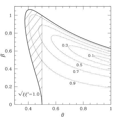
Figure 1: Left panel: stability region in the ($\theta,\beta$) plane for the two-iterations $\theta$-ICN for the advection equation (8). Thick solid lines mark the limit at which $|\xi|=1$, while the dotted contours indicate the values of the amplification factor in the stable region. The shaded area for $\theta<1/2$ refers to solutions that are linearly unstable [8]. Right panel: same as in the left panel but when the averages between two corrections are swapped. Note that the amplification factor in this case is less sensitive on $\theta$ and always larger than the corresponding amplification factor in the left panel.

IV.3 Swapped weighted averages

The calculation of the stability of the $\theta$-ICN when the weighted averages are swapped as in eqs. (6) and (7) is somewhat more involved; after some lengthy but straightforward algebra we find the amplification factor to be

$$\xi = 1-2{\rm i}\beta-4\beta^{2}\theta+8{\rm i}\beta^{3}\theta(1-\theta)\;,$$ (14)

which differs from (11) only in that the $\theta^{2}$ coefficient of the ${\cal O}(\beta^{3})$ term is replaced by $\theta(1-\theta)$. The stability requirement $|\xi|\leq 1$ is now expressed as

$$16\beta^{4}\theta^{2}(1-\theta)^{2}-4\beta^{2}\theta(2-3\theta)-2\theta+1\leq 0\;.$$ (15)

Solving the condition (15) with respect to $\beta$ amounts then to requiring that

$$\beta\geq\frac{\sqrt{2-3\theta-\sqrt{4\theta-11\theta^{2}+8\theta^{3}}}}{2(1-\theta)\sqrt{2\theta}}\;,$$ (16a)

$$\beta\leq\frac{\sqrt{2-3\theta+\sqrt{4\theta-11\theta^{2}+8\theta^{3}}}}{2(1-\theta)\sqrt{2\theta}}\;,$$ (16b)

which is again equivalent to $\beta^{2}\leq 1$ when $\theta=1/2$. The corresponding region of stability is shown in right panel of Fig. 1 and should be compared with left panel of the same Figure. Note that the average-swapping has now considerably increased the amplification factor, which is always larger than the corresponding one for the $\theta$-ICN in the relevant region of stability (i.e., for $1/2\leq\theta\leq 1$ ).

V Parabolic equations

We next extend the stability analysis of the $\theta$-ICN to the a parabolic partial differential equation and use as model equation the one-dimensional diffusion equation

$$\frac{\partial u}{\partial t}-D\frac{\partial^{2}u}{\partial x^{2}}=0\;,$$ (17)

where $D$ is a constant coefficient which must be positive for the equation to be well-posed.

Parabolic equations are commonly solved using implicit methods such as the Crank-Nicolson, which is unconditionally stable and thus removes the constraints on the timestep [i.e., $\Delta t\approx{\cal O}(\Delta x^{2})$] imposed by explicit schemes [9]. In multidimensional calculations, however, or when the set of equations is of mixed hyperbolic-parabolic type, implicit schemes can be cumbersome to implement since the resulting system of algebraic equations does no longer have simple and tridiagonal matrices of coefficients. In this case, the most conveniente choice may be to use an explicit method such as the ICN.

Also in this case, the first step in our analysis is the derivation of a finite-difference representation of the right-hand-side of eq. (17) which, at second-order, has the form

$${\boldsymbol{L}}(u^{n}_{j,j\pm 1})=\frac{u^{n}_{j+1}-2u^{n}_{j}+u^{n}_{j-1}}{\Delta x^{2}}+{\cal O}(\Delta x^{2})\;.$$ (18)

V.1 Constant Arithmetic Averages

Next, we consider first the case with constant arithmetic averages (i.e., $\theta=1/2$) and the expression for the amplification factor after $M$-iterations is then purely real and given by

$$^{(M)}\xi=1+2\sum_{n=1}^{M}\left(-\gamma\right)^{n}\;,$$ (19)

where $\gamma\equiv(2D\Delta t/\Delta x^{2})\sin^{2}(k\Delta x/2)$. Requiring now for stability that $\sqrt{\xi^{2}}\leq 1$ and bearing in mind that

$$-1\leq\sum_{n=0}^{M}\left(-\gamma\right)^{n+1}\leq 0\;,\hskip 14.22636pt{\rm for\ \ }\gamma\leq 1\;,$$ (20)

we find that the scheme is stable for any number of iterations provided that $\gamma\leq 1$. Furthermore, because the scheme is second-order accurate from the first iteration on, our suggestion when using the ICN method for parabolic equations is that one iteration should be used and no more. In this case, in particular, the ICN method coincides with a FTCS scheme [9].

Figure 2: Left panel: stability region in the ($\theta,\gamma$) plane for the two-iterations $\theta$-ICN for the diffusion equation (17). Thick solid lines mark the limit at which $\xi^{2}=1$, while the dotted contours indicate the values of the amplification factor in the stable region. Right panel: same as in the left panel but with swapping the averages between two corrections.

Note that the stability condition $\gamma\leq 1$ introduces again a constraint on the timestep that must be $\Delta t\leq\Delta x^{2}/(2D)$ and thus ${\cal O}(\Delta x^{2})$. As a result and at least in this respect, the ICN method does not seem to offer any advantage over other explicit methods for the solution of a parabolic equation .

V.2 Constant Weighted Averages

We next consider the stability of the $\theta$-ICN method but focus our attention on a two-iterations scheme since this is the number of iterations needed in the solution of the parabolic part in a mixed hyperbolic-parabolic equation when, for instance, operator-splitting techniques are adopted [9]. In this case, the amplification factor is again purely real and given by

$$\xi = 1-2\gamma+4\gamma^{2}\theta-8\gamma^{3}\theta^{2}\;,$$ (21)

so that stability is achieved if

$$0\leq\gamma\left(1-2\theta\gamma+4\theta^{2}\gamma^{2}\right)\leq 1~{}.$$ (22)

Since $\gamma>0$ by definition, the left inequality is always satisfied, while the right one is true provided that, for $\gamma<4/3$,

$$\frac{\gamma-\sqrt{\gamma(4-3\gamma)}}{4\gamma^{2}}\leq\theta\leq\frac{\gamma+\sqrt{\gamma(4-3\gamma)}}{4\gamma^{2}}\;.$$ (23)

The stability region described by the condition (23) is shown in the left panel of Fig. 2 for $\sin k\Delta x=1$ and illustrates that the scheme is stable for any value $0\leq\theta\leq 1$, and also that slightly larger timesteps can be taken when $\theta\simeq 0.2$.

V.3 Swapped Weighted Averages

After some lengthy algebra the calculation of the amplification factor for the $\theta$-ICN method with swapped weighted averages yields

$$\xi=1-2\gamma+4\gamma^{2}\theta-8\gamma^{3}\theta(1-\theta)\;,$$ (24)

and stability is then given by

$$-1\leq 1-2\gamma+4\gamma^{2}\theta-8\gamma^{3}\theta(1-\theta)\leq 1\;.$$ (25)

Note that none of the two inequalities is always true and in order to obtain analytical expressions for the stable region we solve the condition (25) with respect to $\theta$ and obtain

$$\theta\leq\frac{2\gamma-1+\sqrt{4\gamma^{2}-4\gamma+5}}{4\gamma}~{},$$ (26a)

$$\theta\leq\frac{\gamma(2\gamma-1)-\sqrt{\gamma\left(4\gamma^{3}-4\gamma^{2}+5\gamma-4\right)}}{4\gamma^{2}}\;,$$ (26b)

$$\theta\geq\frac{\gamma(2\gamma-1)+\sqrt{\gamma\left(4\gamma^{3}-4\gamma^{2}+5\gamma-4\right)}}{4\gamma^{2}}\;.$$ (26c)

The resulting stable region for $\sin k\Delta x=1$ is plotted in the right panel of Fig. 2 and seems to suggest that arbitrarily large values of $\gamma$ could be considered when $\theta\gtrsim 0.6$ It should be noted, however, that the amplification factor is also severely reduced as larger values of $\gamma$ are used and indeed it is essentially zero in the limit $\theta\to 1$.

VI Truncation error, dissipation and dispersion

Although not often appreciated, the $\theta$-ICN method is only first-order accurate in time as an obvious consequence of the first-order approximation in the time derivative [cf. eq. (2)]. However, this is not true if $\theta=1/2$, in which case the method becomes second-order in both space and time.

To appreciate this in the case of the advection equation (8), we report the finite-difference expressions for the time and spatial derivatives in eq. (8), writing out explicitly the coefficients of the ${\cal O}(\Delta t)$ and ${\cal O}(\Delta x^{2})$ terms

$$\frac{u^{n+1}_{j}-u^{n}_{j}}{\Delta t}=\left.\frac{\partial u}{\partial t}\right|_{n,j}\!\!\!+\left.\frac{1}{2}\frac{\partial^{2}u}{\partial t^{2}}\right|_{n,j}\!\!\!\!\!\!\Delta t+{\cal O}\left(\Delta t^{2}\right)\;,$$ (27)

$$\frac{u^{n}_{j+1}-u^{n}_{j-1}}{2\Delta x}=\left.\frac{\partial u}{\partial x}\right|_{n,j}\!\!\!+\left.\frac{1}{6}\frac{\partial^{3}u}{\partial x^{3}}\right|_{n,j}\!\!\!\!\!\!\Delta x^{2}+{\cal O}(\Delta x^{4})\;.$$

The resulting local truncation error is then

$$e_{{}_{\rm T}} = \left(\frac{1}{2}-\theta\right)v\left.\frac{\partial^{2}u}{\partial x\partial t}\right|_{n,j}\!\!\!\!\!\!\Delta t-\frac{v}{6}\left.\frac{\partial^{3}u}{\partial x^{3}}\right|_{n,j}\!\!\!\!\!\!\Delta x^{2}$$ (29)

$$-v^{3}\theta^{2}\left.\frac{\partial^{3}u}{\partial x^{3}}\right|_{n,j}\!\!\!\!\!\!\Delta t^{2}-\frac{1}{6}\left.\frac{\partial^{3}u}{\partial t^{3}}\right|_{n,j}\!\!\!\!\!\!\Delta t^{2}$$

$$+\ {\cal O}\left(\Delta t^{3},\Delta x^{3}\right)~{},$$

clearly indicating that the $\theta$-ICN is generally only first-order accurate in time, becoming second-order if $\theta=1/2$. The truncation error is also useful to quantify the numerical dissipation and dispersion inherent to the $\theta$-ICN method. Using eq. (8) to replace the time derivative with a spatial one, in fact, eq. (29) shows that the $\theta$-ICN introduces a dissipative term proportional to $\partial^{2}u/\partial x^{2}$ and with coefficient

$$\epsilon_{\rm adv}=\left(\theta-\frac{1}{2}\right)v^{2}\Delta t~{}.$$ (30)

In other words, the $\theta$-ICN is intrinsically dissipative, with a dissipation coefficient that is generically ${\cal O}(\Delta t)$ and ${\cal O}(\Delta t^{3},\Delta x^{3})$ only when $\theta=1/2$. Furthermore, it is now apparent why $\theta$ must be larger or equal to $1/2$; any choice different from this, in fact, would change the sign of $\epsilon_{\rm adv}$, leading to an ill-posed equation with exponentially growing solutions [cf. eq. (17)].

Expression (30) also clarifies the behaviour found in refs. [2, 3]. Since stability in a numerical scheme is either gained or lost but cannot be “improved”, the use of a weighting coefficient $\theta>1/2$ (and of a suitable timestep) has simply the effect of increasing the numerical dissipation of the scheme. Of course, this is often a desirable feature to suppress the growth of instabilities, as in the case of the Lax-Friedrichs scheme, whose numerical dissipation stabilizes the otherwise unconditionally unstable FTCS scheme [9].

An alternative route to a second-order, moderately dissipative scheme is to choose

$$\theta=\frac{1}{2}+\frac{\Delta x^{2}}{v\Delta t}\;,$$ (31)

with ${\Delta x^{2}}/({v\Delta t})\leq 1/2$, so that the leading error-term in (29) becomes again ${\cal O}(\Delta t^{2},\Delta x^{2})$. A prescription of the type (31) may be the optimal one for the $\theta$-ICN method as it provides a small amount of numerical dissipation and reduces the truncation error.

The truncation error (29) also indicates that the $\theta$-ICN introduces a dispersive term proportional to $\partial^{3}u/\partial x^{3}$ given by

$$\chi_{\rm adv}=\left(\frac{1}{6}-\theta^{2}-\frac{1}{24\beta^{2}}\right)v^{3}\Delta t^{2}\;,$$ (32)

and responsible, for instance, for different propagation speeds of the Fourier modes in the initial data (i.e., phase drifts).

All what discussed so far for the $\theta$-ICN scheme continues to hold also when the averages are swapped, the only difference being that the dispersive contribution is instead given by

$$\chi_{\rm adv}=\left(\frac{1}{6}-\theta+\theta^{2}-\frac{1}{24\beta^{2}}\right)v^{3}\Delta t^{2}\;,$$ (33)

and is therefore smaller for $\theta>1/2$, making this variant to the $\theta$-ICN preferable overall.

Similar calculations can be carried out also for the parabolic equation (17) and the local truncation error in this case is

$$e_{{}_{\rm T}}=\left(\theta-\frac{1}{2}\right)D\left.\frac{\partial^{3}u}{\partial t\partial x^{2}}\right|_{n,j}\!\!\!\!\!\!\Delta t+{\cal O}\left(\Delta t^{2},\Delta x^{2}\right)\;,$$ (34)

indicating that mathematically the $\theta$-ICN is again only first-order accurate in time, with second-order accuracy being recovered for $\theta=1/2$. However, stability requires that $\Delta t={\cal O}\left(\Delta x^{2}\right)$ (cf. Sect. V.1) and thus the truncation error is effectively $e_{{}_{\rm T}}={\cal O}\left(\Delta x^{2}\right)$ for all of the allowed values $0\leq\theta\leq 1$.

Finally, using eq. (17) to the replace the time derivative in (34) shows that the $\theta$-ICN for a parabolic equation has an additional dissipative term proportional to $\partial^{4}u/\partial x^{4}$ with coefficient

$$\epsilon_{\rm diff}=\left(\theta-\frac{1}{2}\right)D^{2}\Delta t\;,$$ (35)

which is again zero only for $\theta=1/2$.

Figure 3: Upper panel: Solution of the advection equation (8) using the $\theta$-ICN method and shown after 10 crossing times. Different curves refer to either the analytic solution or to the numerical ones with different weighting coefficients. The small inset, instead, shows the smaller diffusion and dispersion obtained when the averages are swapped (see main text for details). Lower panel: L₂ norms of the solutions in the upper panel plotted as a function of time.

As a purely representative example we show in Fig. 3 the application of the $\theta$-ICN method for the solution of the advection equation (8) with $v=1$ and $\beta=0.6$ (cf. Fig. 1). The numerical domain has length $1.0$ and was covered with 200 equally spaced gridpoints. The initial solution, given by a Gaussian centred at $x=0.5$ and with variance $0.1$, was evolved for $10$ crossing times using periodic boundary conditions. Different curves in the upper panel refer to either the analytic solution at the final time (dotted line) or to the numerical solutions as obtained with different weighting coefficients. Note that already with $\theta=1/2$ (solid line) the numerical solution is slightly diffused but suffers from considerable dispersion as apparent from the considerable “delay” and the presence of negative values to the left of the maximum. These dispersion errors can be reduced if larger values of the weighting coefficients are used as indicated by the short-dashed and long-dashed lines referring to $\theta=0.6$ and $\theta=0.8$, respectively. This improvement, however, also comes with a larger dissipation and truncation error (as mentioned in Sect. VI, the system is just first-order in time with $\theta>1/2$) . This is particularly evident when considering the evolution of the L₂ norms of the solutions as reported in the lower panel of Fig. 3. It is interesting to note that for $\theta=0.8$ the L₂ norm of the solution has been reduced of about 25% after 10 crossing times, while this decrease is less than 1% when $\theta=1/2$.

Finally, the two small insets in Fig. 3 offer a comparison in the solutions for $\theta=0.6$ when the coefficients in the averages are either held constant (short-dashed lines) or swapped between two subsequent corrector steps (dot-dashed lines). Although the difference is rather small for the selected set of parameters, it is evident that the swapping of the coefficients has the effect of decreasing both the dispersion (the dot-dashed line in the upper inset has a smaller “delay”) and the diffusion (at any given time the dot-dashed line in the lower inset has a larger value).

VII Conclusions

We have extended the recent work on the properties of the ICN scheme for hyperbolic equations by investigating the stability properties when it is treated as a $\theta$-method, i.e., when the average between the predicted and corrected values is made with unequal weights. In addition we have studied the properties of the $\theta$-ICN method for a model parabolic equation and proposed a variant of the scheme, valid for both hyperbolic and parabolic equations, in which the unequal coefficients coefficients in the averages are swapped between two subsequent corrector steps. This novel approach leads to amplification factors that are systematically larger than those found in the $\theta$-ICN method and to a smaller numerical dispersion.

Overall, our results indicate that although generally only first-order accurate in time, the $\theta$-ICN method is a flexible approach to the time-integration of partial differential equations, particularly when these are of mixed hyperbolic-parabolic type. Because the use of unequal coefficients in the average provides a small but nonzero amount of numerical dissipation, this could prove useful in numerical relativity calculations which may suffer from the development of numerical instabilities and for which lower-order evolution schemes are an acceptable compromise between accuracy and stability.

References

- Teukolsky [2000] S. A. Teukolsky, Phys. Rev. D 61 (2000).
- Duez et al. [2003] M. D. Duez, P. Marronetti, S. L. Shapiro, and T. W. Baumgarte, Phys. Rev. D 67, 024004 (2003).
- Duez et al. [2004] M. D. Duez, Y. T. Liu, S. L. Shapiro, and B. C. Stephens, Phys. Rev. D 69, 104030 (2004).
- Calabrese et al. [2005] G. Calabrese, I. Hinder, and S. Husa (2005), eprint gr-qc/0503056.
- Crank and Nicolson [1947] J. Crank and P. Nicolson, Proc. Camb. Philos. Soc. 43, 50 (1947).
- Richtmyer and Morton [1967] R. D. Richtmyer and K. W. Morton, Difference Methods for Initial-Value Problems (John Wiley & Sons, 1967), 2nd ed.
- Stuart and Peplow [1991] A. M. Stuart and A. T. Peplow, SIAM Journal on Scientific and Statistical Computing 12, 1351 (1991).
- Barclay et al. [2000] G. J. Barclay, D. F. Griffiths, and D. J. Higham, LMS Journal of Computation and Mathematics 3, 27 (2000).
- Press et al. [1997] W. H. Press, S. A. Teukolsky, W. T. Vetterling, and B. P. Flannery, Numerical Recipes (Cambridge Univesity Press, 1997).
- Du-Fort and Frankel [1953] E. C. Du-Fort and S. P. Frankel, Mathematical Tables and Other Aids to Computation 7, 135 (1953).
- Smith [1986] G. D. Smith, Numerical Solution of Partial Differential Equations: Finite Difference Methods (Oxford Univesity Press, 1986), 3rd ed.