Spectral Line Broadening and Angular Blurring due to Spacetime Geometry Fluctuations

Abstract

We treat two possible phenomenological effects of quantum fluctuations of spacetime geometry: spectral line broadening and angular blurring of the image of a distance source. A geometrical construction will be used to express both effects in terms of the Riemann tensor correlation function. We apply the resulting expressions to study some explicit examples in which the fluctuations arise from a bath of gravitons in either a squeezed state or a thermal state. In the case of a squeezed state, one has two limits of interest: a coherent state which exhibits classical time variation but no fluctuations, and a squeezed vacuum state, in which the fluctuations are maximized.

I Introduction

Spacetime fluctuations are expected to be a generic feature of a theory which combines quantum theory and gravitation. While there is still no complete quantum theory of gravity, it is possible to investigate some of the characteristics expected of fluctuating spacetime geometries. One can roughly classify these fluctuations as being either active or passive. Active fluctuations arise from fluctuations of the dynamical degrees of freedom of gravity itself, that is, from the quantization of gravity. Passive fluctuations arise from fluctuations in the stress tensor due to quantum matter fields. In general, one expects both types of fluctuations to be present. One approach to the study of fluctuating spacetimes is stochastic gravity Stochastic . More generally, there has been considerable activity in recent years in the area of quantum gravity phenomenology, which seeks to find observational signatures of the quantum nature of spacetime Moffat ; JR94 ; GLF ; HS97 ; EMN00 ; NvD00 ; AC00 ; NCvD03 ; AC04 ; DHR04 ; Borgman . There has also been considerable attention given to the effects of classical stochastic gravitational fields Zipoy ; Sachs ; Kaufmann ; BM71 ; BKPN90 and to scattering of probe particles by gravitons in an S-matrix approach Weber ; DeWitt .

Spacetime geometry fluctuations should in principle produce observable effects on test particles, such as light rays. Several effects of fluctuating gravitational fields on light propagation have been discussed by previous authors. For example, Sachs and Wolfe Sachs treated the scattering of cosmic microwave photons from cosmological density perturbations. Zipoy Zipoy argued that there will be apparent luminosity variations in a source seen through a stochastic gravitational field. More recently, this effect has been treated Borgman using a Langevin form of the Raychaudhuri equation Moffat . In the latter approach, luminosity fluctuations are a signature of passive spacetime geometry fluctuations caused by quantum stress tensor fluctuations. Zipoy Zipoy also examined changes in angular position due to a stochastic gravitational field. Kaufman Kaufmann considered redshift fluctuations from a bath of gravity waves. If one goes beyond the geometric optics approximation to consider electromagnetic waves propagating in a stochastic gravitational field, there will be phase shift variations BM71 ; BKPN90 ; HS97 .

The purpose of the present paper is to analyze in more detail two particular signatures of spacetime geometry fluctuations, redshift fluctuations and angular blurring of images. We derive simple expressions involving the Riemann tensor correlation function and use these to examine fluctuations in redshift and angular position of a source. We will illustrate this approach using the cases of gravitons in a squeezed state and in a thermal state, and calculate the broadening of spectral lines and an angular blurring of an object viewed through a region of spacetime filled with gravitons. This will serve as a simple example of spacetime undergoing active quantum fluctuations.

This paper is organized as follows: In Sect. II we provide a detailed derivation of the equations for redshift fluctuations and angular blurring given in Ref. peyresq10 . The derivation is independent of the source of fluctuations, being based on the Riemann tensor correlation function. In Sect. III we assume that gravitons in a general squeezed state act as the source of fluctuations and are described by the correlation function, and we then specialize the results from Sect. II to this model. Several examples are calculated for the variance of both redshift and angular position, and are compared with the expected classical time variation of these quantities. We then express these results in terms of the energy density of the gravity wave and make an order of magnitude estimate for the size of the effect. In Sect. IV we assume a thermal bath of gravitons as the source of fluctuations and again specialize the results of Section II to this model. The results of the paper are summarized and discussed in Sect. V. A brief review of the pertinent information regarding squeezed quantum states required for this paper can be found in the appendix. Units in which $G=\hbar=c=1$ will be used, where $G$ is Newton’s constant.

II Redshift and Angular Blurring in Linearized Gravity

II.1 Linearized Redshift

Let $t^{\mu}$ be the 4-velocity of a source and $v^{\mu}$ the 4-velocity of a detector at the events of emission and absorption, respectively, and let $k^{\mu}$ be tangent to the null geodesic connecting them (see Fig. 1, e.g., path $DA$). Let $\lambda$ be an affine parameter that runs from $\lambda=0$ (emission) to $\lambda=\lambda_{0}$ (absorption). Since $k^{\mu}$ is tangent to a geodesic,

$$\frac{dk^{\mu}}{d\lambda}+\Gamma^{\mu}_{\alpha\beta}k^{\alpha}k^{\beta}=0$$ (1)

and so

$$k^{\mu}(\lambda)=k^{\mu}(0)-\int_{0}^{\lambda}d\lambda^{\prime}\,\Gamma^{\mu}_{\alpha\beta}(\lambda^{\prime})k^{\alpha}(\lambda^{\prime})k^{\beta}(\lambda^{\prime}).$$ (2)

This is an integral equation for $k^{\mu}(\lambda)$, but in the linearized theory, we let $k^{\mu}(\lambda^{\prime})\approx k^{\mu}(0)$ on the right hand side. So at the point of detection,

$$k^{\mu}(\lambda_{0})=k^{\mu}(0)-\int_{0}^{\lambda_{0}}d\lambda^{\prime}\,\Gamma^{\mu}_{\alpha\beta}(\lambda^{\prime})k^{\alpha}(0)k^{\beta}(0).$$ (3)

The frequency of emission is proportional to $-k^{\mu}t_{\mu}$. The proportionality constant depends on the choice of affine parameter. If we choose the affine parameter such that, for example, $k^{\mu}=(\omega,\omega,0,0)$ in the rest frame of the source, then $\omega=-t_{\mu}k^{\mu}.$ Since Eq. (1) is scale invariant, we may also select an affine parametrization such that $k^{\mu}=(1,1,0,0).$ This amounts to choosing the affine parameter to coincide with the source’s proper time at the evaluation point. We adopt the latter parametrization of $\lambda$, in which case the ratio of the detected to the emitted frequency is

$$\frac{\omega(\lambda_{0})}{\omega_{0}}=-v_{\mu}k^{\mu}(\lambda_{0})=-v_{\mu}k^{\mu}(0)+v_{\mu}\int_{0}^{\lambda_{0}}d\lambda^{\prime}\,\Gamma^{\mu}_{\alpha\beta}(\lambda^{\prime})k^{\alpha}(0)k^{\beta}(0)\,,$$ (4)

where $\omega_{0}=\omega(0)$ is the emitted frequency. The first term on the right hand side of this equation can be written as

$$-v_{\mu}k^{\mu}(0)=-t_{\mu}k^{\mu}(0)-(v_{\mu}-t_{\mu})k^{\mu}(0)=1-(v_{\mu}-t_{\mu})k^{\mu}(0).$$ (5)

With this, the fractional change in detected frequency between source and detector is

$$\frac{\Delta\omega}{\omega_{0}}=\frac{\omega(\lambda_{0})-\omega_{0}}{\omega_{0}}=-(v_{\mu}-t_{\mu})k^{\mu}(0)+v_{\mu}\int_{0}^{\lambda_{0}}d\lambda^{\prime}\,\Gamma^{\mu}_{\alpha\beta}(\lambda^{\prime})k^{\alpha}(0)k^{\beta}(0).$$ (6)

The first term on the right hand side is a Doppler shift which may not be zero even in flat space. The second term is a linearized gravitational redshift which depends on the intermediate geometry between source and detector. We will focus our attention on this second term.

Figure 1: A source moves along a worldline with tangent $t^{\mu}$ while a detector a proper distance $s$ away moves along a worldline with tangent $v^{\mu}$. The source emits a ray at point D which has tangent $k^{\mu}(\lambda=0)$ at point D and tangent $k^{\mu}(\lambda_{0})$ at A. Parallel propagation of $k^{\mu}$ around ABCD results in a slightly rotated vector $k^{\mu}+\Delta k^{\mu}$. The closed path ABCD encloses the spacetime region of interest.

II.2 Rate of Change of Redshift

The next step is to examine the rate of change of the redshift. We examine the behavior of successive photons emitted from the source. Our interest lies in the change in frequency due to the effects of gravity rather than as a result of a variation of the output of the source. This condition is enforced by requiring that the values of $k^{\mu}$ at the start of any two null geodesics are related by parallel transport along the worldline of the source. Thus we assume that $\omega_{0}$ is constant between successive emissions and want to find $\dot{\omega}(\lambda_{0})$ at the detector due to changes in spacetime geometry. Initially at the detector,

$$\omega(\tau_{1},\lambda_{0})=-v_{\mu}(\tau_{1})k^{\mu}(\tau_{1},\lambda_{0})\,\omega_{0}$$ (7)

is the frequency at the detector at proper time $\tau_{1}$. While after a time $\Delta\tau$, at proper time $\tau_{2}$, the frequency at the detector is

$$\omega(\tau_{2},\lambda_{0})=-v_{\mu}(\tau_{2})k^{\mu}(\tau_{2},\lambda_{0})\,\omega_{0}\,.$$ (8)

To find $v^{\mu}(\tau_{2})$, we first note that $v^{\mu}$ is tangent to a geodesic:

$$\frac{dv^{\mu}}{d\tau}+\Gamma^{\mu}_{\alpha\beta}v^{\alpha}v^{\beta}=0\,,$$ (9)

so

$$v^{\mu}(\tau_{2})-v^{\mu}(\tau_{1})\approx\frac{dv^{\mu}}{d\tau}\Delta\tau\simeq-\Gamma^{\mu}_{\alpha\beta}v^{\alpha}v^{\beta}\Delta\tau.$$ (10)

This depends on $\Gamma^{\mu}_{\alpha\beta}$ at the location of the detector. For simplicity, we assume $\Gamma^{\mu}_{\alpha\beta}=0$ at the location of the detector. This can be achieved by assuming the detector is located in a flat region; more will be said about this in the next subsection. Thus $v^{\mu}(\tau_{2})=v^{\mu}(\tau_{1})=v^{\mu}.$

To find the change in $k^{\mu}$, we parallel transport the vector around the closed path ABCD (see Fig. 1). Recall that if we parallel transport a vector around a closed path, the change in the vector can be expressed as an integral of the Riemann tensor over the area enclosed by the path. For parallel transport around an infinitesimal parallelogram, we have for an arbitrary vector $V^{\mu}$

$$V^{\mu}\rightarrow V^{\mu}+\delta V^{\mu}\,,$$ (11)

where

$$\delta V^{\mu}=-R^{\mu}_{\phantom{\mu}\alpha\nu\beta}V^{\alpha}t^{\nu}k^{\beta}\Delta\lambda\Delta\tau.$$ (12)

Integrating over $\lambda$ and $\tau$ transports $V^{\mu}$ around a finite parallelogram so that

$$\Delta V^{\mu}=-\int d\tau\int d\lambda\,R^{\mu}_{\phantom{\mu}\alpha\nu\beta}V^{\alpha}t^{\nu}k^{\beta}.$$ (13)

Since we assume the detector is located in a flat region, we can further assume that $k^{\mu}$ may be trivially transported from point $A$ to point $B$, and we have

$$k^{\mu}(\tau_{1},\lambda_{0})+\Delta k^{\mu}=k^{\mu}(\tau_{2},\lambda_{0})\,.$$ (14)

Thus

$$\Delta k^{\mu}=k^{\mu}(\tau_{2},\lambda_{0})-k^{\mu}(\tau_{1},\lambda_{0})=-\int_{\tau_{1}}^{\tau_{2}}d\tau\int_{0}^{\lambda_{0}}d\lambda\,R^{\mu}_{\phantom{\mu}\alpha\nu\beta}k^{\alpha}t^{\nu}k^{\beta}\,,$$ (15)

and from Eqs. (7) and (8)

$$\frac{\Delta\omega(\lambda_{0})}{\omega_{0}}=\frac{\omega(\tau_{2},\lambda_{0})-\omega(\tau_{1},\lambda_{0})}{\omega_{0}}=-v_{\mu}\Delta k^{\mu}=v_{\mu}\int_{\tau_{1}}^{\tau_{2}}d\tau\int_{0}^{\lambda_{0}}d\lambda\,R^{\mu}_{\phantom{\mu}\alpha\nu\beta}k^{\alpha}t^{\nu}k^{\beta}.$$ (16)

This equation can be thought of as relating the difference between taking path DAB and path DCB. Taking limits in the previous equation yields the rate of change of the fractional redshift in the linearized theory:

$$\frac{d}{d\tau}\left(\frac{\omega(\lambda_{0})}{\omega_{0}}\right)=v_{\mu}\int_{0}^{\lambda_{0}}d\lambda\,R^{\mu}_{\phantom{\mu}\alpha\nu\beta}k^{\alpha}t^{\nu}k^{\beta}.$$ (17)

An equivalent formula has been obtained by Braginsky and Menskii BM71 using the geodesic deviation equation.

II.3 Fluctuating Redshift

Now suppose the Riemann tensor is subject to fluctuations - active, passive, or both. We first have to specify $t^{\mu}$ and $v^{\mu}$ and how they behave under the fluctuations. The simplest assumption is that $t^{\mu}$ and $v^{\mu}$ do not fluctuate, and in the underlying flat geometry $v^{\mu}=t^{\mu}$. Physically, this might be achieved via several methods. We have already mentioned that we can assume the detector to be located in a flat region. However, one could also consider the source and the detector rigidly attached to one another by non-gravitational forces. The same effect might be achieved if the source and detector are separately attached to platforms (e.g. planets) which are large enough that they travel on an average geodesic in the mean spacetime. This can happen if the spatial average of the fluctuations over the platform is small. For our purposes it is sufficient to assume the perturbation vanishes at both the source and detector, e.g., a gravity wave passes between source and detector, but far from either source or detector; so we can assume the source and detector to be located in flat regions. The fluctuations of the Riemann tensor are described by the correlation function

$$C_{\alpha\beta\mu\nu\,\gamma\delta\rho\sigma}(x,x^{\prime})=\langle R_{\alpha\beta\mu\nu}(x)R_{\gamma\delta\rho\sigma}(x^{\prime})\rangle-\langle R_{\alpha\beta\mu\nu}(x)\rangle\langle R_{\gamma\delta\rho\sigma}(x^{\prime})\rangle,$$ (18)

where the indices $\alpha\beta\mu\nu$ refer to point $x$ while the indices $\gamma\delta\rho\sigma$ refer to point $x^{\prime}$. With $v^{\mu}=t^{\mu}$, we get from Eq. (6)

$$\xi\equiv\frac{\Delta\omega}{\omega_{0}}=\frac{\omega(\lambda_{0})-\omega_{0}}{\omega_{0}}=\int_{0}^{\lambda_{0}}d\lambda\,\Gamma^{\mu}_{\alpha\beta}(\lambda)k^{\alpha}(0)k^{\beta}(0)t_{\mu}.$$ (19)

We let $\Gamma^{\mu}_{\alpha\beta}$ fluctuate with fixed $k^{\alpha}=k^{\alpha}(0)$ and $t_{\mu},$ so that

$$\langle\xi\rangle=\int_{0}^{\lambda_{0}}d\lambda\,\langle\Gamma^{\mu}_{\alpha\beta}(\lambda)\rangle k^{\alpha}k^{\beta}t_{\mu}.$$ (20)

The integral in this equation is evaluated along a single line, e.g., along the paths DA or CB. The equation may be interpreted in the following way: Suppose the spacetime is subject to quantum fluctuations. Then, given an ensemble of systems, measurement of the fractional redshift along the same line will yield different results. This equation gives the expectation value of those measurements. Therefore, comparing the result of an integration along path DA with that along path CB will give the expectation of the difference of the fractional redshifts. Another, more convenient way to obtain the same information is via Eq. (17). Notice that

$$\frac{d\xi}{d\tau}=\frac{d}{d\tau}\left(\frac{\omega(\lambda_{0})-\omega_{0}}{\omega_{0}}\right)=\frac{d}{d\tau}\left(\frac{\omega(\lambda_{0})}{\omega_{0}}\right)\,,$$ (21)

and thus from (17),

$$\frac{d\xi}{d\tau}=\int_{0}^{\lambda_{0}}d\lambda\,R_{\alpha\beta\mu\nu}(\tau,\lambda)t^{\alpha}k^{\beta}t^{\mu}k^{\nu}.$$ (22)

Integrating this expression yields

$$\Delta\xi=\xi\bigr{|}_{\tau_{2}}-\xi\bigr{|}_{\tau_{1}}=\int_{\tau_{1}}^{\tau_{2}}d\tau\int_{0}^{\lambda_{0}}d\lambda\,R_{\alpha\beta\mu\nu}(\tau,\lambda)t^{\alpha}k^{\beta}t^{\mu}k^{\nu}.$$ (23)

We now let $R_{\alpha\beta\mu\nu}(\tau,\lambda)$ fluctuate, and find the expectation value $\langle\Delta\xi\rangle$ is

$$\langle\Delta\xi\rangle=\int_{\tau_{1}}^{\tau_{2}}d\tau\int_{0}^{\lambda_{0}}d\lambda\,\langle R_{\alpha\beta\mu\nu}(\tau,\lambda)\rangle t^{\alpha}k^{\beta}t^{\mu}k^{\nu}.$$ (24)

The expectation of the square, $\langle(\Delta\xi)^{2}\rangle$, is related to the line broadening an observer will see. Recall that $\xi$ is the fractional change in frequency of an observed spectral line, the fractional redshift. Upon quantizing the perturbation between source and detector we strictly must discuss the fractional redshift along a given path as an ensemble average. An observer, over some proper time interval $\Delta\tau$, collects information on a distribution of fractional redshifts; $\langle(\Delta\xi)^{2}\rangle$ is the squared width of this distribution. The physical realization of this measurement is a broadening of the observed spectral line.

However, there is a contribution to spectral line broadening due to regular time dependent variations of the spacetime, for example as a result of passing classical gravity waves. We thus characterize the fluctuation of redshift about the classical time dependent variation that arises from a nonzero expectation value of the Riemann tensor. Using Eq. (18), we can express the variance of the fractional redshift, $\delta\xi^{2}$, as

$$\delta\xi^{2}=\langle(\Delta\xi)^{2}\rangle-\langle\Delta\xi\rangle^{2}=\int da\int da^{\prime}\,C_{\alpha\beta\mu\nu\,\gamma\delta\rho\sigma}(x,x^{\prime})t^{\alpha}k^{\beta}t^{\mu}k^{\nu}t^{\gamma}k^{\delta}t^{\rho}k^{\sigma}.$$ (25)

The integration over the spacetime region $\int da$ corresponds to $\int_{\tau_{1}}^{\tau_{2}}d\tau\int_{0}^{\lambda_{0}}d\lambda$ and similarly for $da^{\prime}$. This is an integration over the spacetime region enclosed by the path ABCD in Fig. 1. The point $x$ corresponds to the point $(\tau,\lambda)$ and similarly for $x^{\prime}$.

II.4 Fluctuating Angular Position

We can also relate the degree of angular blurring of the source observed by the detector to the Riemann tensor correlation function. Let $s^{\mu}$ be a unit spacelike vector in a direction orthogonal to the direction of propagation of the null rays; thus $s_{\mu}t^{\mu}=s_{\mu}k^{\mu}(\lambda=0)=0$. Then at the observation point

$$s_{\mu}k^{\mu}(\lambda_{0})=\tan\Theta\approx\Theta,$$ (26)

where $\Theta$ is an angle in the plane defined by the pair of spacelike vectors $s^{\mu}$ and $n^{\mu}=k^{\mu}-t^{\mu}$ and is assumed to be small, $|\Theta|\ll 1$. The angle $\Theta$ is the angular deviation in the direction of $s^{\mu}$ of the image of the source from its classical flat space position. A treatment similar to that shown for fractional redshift allows us to express the change in angle, $\Delta\Theta$, in terms of an integral of the Riemann tensor as

$$\Delta\Theta=s_{\mu}\Delta k^{\mu}=\int da\,R_{\alpha\beta\mu\nu}s^{\alpha}k^{\beta}t^{\mu}k^{\nu}.$$ (27)

A fluctuating spacetime results in an ensemble distribution of image positions about the classical flat space position. Analogously to the line broadening effects, the fluctuating angular position manifests itself as a blurring of the source’s image. $\langle(\Delta\Theta)^{2}\rangle$ is therefore a measure of the angular size of the image. The variance of $\Delta\Theta$, $\delta\Theta^{2}$, due to fluctuations in the Riemann tensor is

$$\delta\Theta^{2}=\langle(\Delta\Theta)^{2}\rangle-\langle\Delta\Theta\rangle^{2}=\int da\int da^{\prime}\,C_{\alpha\beta\mu\nu\,\gamma\delta\rho\sigma}(x,x^{\prime})s^{\alpha}k^{\beta}t^{\mu}k^{\nu}s^{\gamma}k^{\delta}t^{\rho}k^{\sigma}.$$ (28)

II.5 Quantization of the Riemann Tensor

Our key results for the redshift fluctuations, Eq. (25), and for the angular blurring, Eq. (28), apply both to active and passive fluctuations of spacetime geometry. We will present some explicit examples for the case of active fluctuations. We examine fluctuations produced by gravitons occupying a squeezed state and then a thermal bath of gravitons in the following two sections, respectively. First we describe some of the formalism relevant to both cases. A linearized quantum field theory for gravity is used, with the field operator expanded as

$$\hat{h}_{\mu\nu}=\sum_{\ell,p}\left(A_{\mu\nu}\hat{a}_{\ell,p}e^{i\ell_{\tau}x^{\tau}}+h.c.\right)\,,$$ (29)

where $\ell^{\mu}$ is the wavevector and $p$ labels the polarization of a mode with polarization tensor $A_{\mu\nu}=A_{\mu\nu}(\ell,p)$. In this theory, the Riemann tensor operator is given by

$$\hat{R}_{\alpha\beta\mu\nu}(x)=\partial_{\nu}\partial_{[\alpha}\hat{h}_{\beta]\mu}-\partial_{\mu}\partial_{[\alpha}\hat{h}_{\beta]\nu}.$$ (30)

Here the convention for antisymmetrization as found in Ref. MTW is used, i.e. $\partial_{\nu}\partial_{[\alpha}h_{\beta]\mu}=\frac{1}{2}(\partial_{\nu}\partial_{\alpha}h_{\beta\mu}-\partial_{\nu}\partial_{\beta}h_{\alpha\mu})$. Henceforth $h_{\mu\nu}$ and $R_{\alpha\beta\mu\nu}$ are understood to be operators, and the hat may be suppressed without confusion. The expectation value of $R_{\alpha\beta\mu\nu}$ is

$$\langle R_{\alpha\beta\mu\nu}(x)\rangle=\langle\partial_{\nu}\partial_{[\alpha}h_{\beta]\mu}\rangle-\langle\partial_{\mu}\partial_{[\alpha}h_{\beta]\nu}\rangle\,.$$ (31)

It is convenient to define

$$K_{\alpha\beta\mu\nu\,\gamma\delta\rho\sigma}(x,x^{\prime}) = \langle\partial_{\nu}\partial_{\alpha}h_{\beta\mu}(x)\partial_{\sigma}^{\prime}\partial_{\gamma}^{\prime}h_{\delta\rho}(x^{\prime})\rangle-\langle\partial_{\nu}\partial_{\alpha}h_{\beta\mu}(x)\rangle\langle\partial_{\sigma}^{\prime}\partial_{\gamma}^{\prime}h_{\delta\rho}(x^{\prime})\rangle$$ (32)

$$= \partial_{\nu}\partial_{\alpha}\partial_{\sigma}^{\prime}\partial_{\gamma}^{\prime}\left(\langle h_{\beta\mu}(x)h_{\delta\rho}(x^{\prime})\rangle-\langle h_{\beta\mu}(x)\rangle\langle h_{\delta\rho}(x^{\prime})\rangle\right)\,,$$

where $\partial^{\prime}$ denotes differentiation with respect to $x^{\prime}$. The Riemann tensor correlation function may be expressed as

$$C_{\alpha\beta\mu\nu\,\gamma\delta\rho\sigma}(x,x^{\prime})=4K_{[\alpha\beta][\mu\nu]\,[\gamma\delta][\rho\sigma]}(x,x^{\prime})\,.$$ (33)

III Gravitons in a Squeezed State

III.1 Single Mode Squeezed State

Gravitons in a squeezed state are the natural result of quantum graviton creation in a background gravitational field, such as in an expanding universe GS90 . Here we suppose that the region between a source and a detector is filled with gravitons in a squeezed state, which produce spacetime geometry fluctuations. A brief summary of the properties of squeezed states needed for the following calculations may be found in the appendix. To calculate $C_{\alpha\beta\mu\nu\,\gamma\delta\rho\sigma}(x,x^{\prime})$, we must calculate $\langle h_{\beta\mu}(x)h_{\delta\rho}(x^{\prime})\rangle$ and $\langle h_{\beta\mu}(x)\rangle$. We are interested in the change in quantum fluctuations between the vacuum state and a squeezed state, so we may take the correlation function to be normal-ordered. We choose to evaluate the expectation value with respect to a gravity wave in a general single mode squeezed state $|\alpha,\zeta\rangle$ (see the appendix), where $\alpha$ and $\zeta$ are the displacement and squeeze parameters, respectively, and the only mode excited has a specific wave vector $\ell^{\mu}$, frequency $\omega_{g}=\ell^{0}$ and polarization $p$. We may now proceed to calculate $\langle\zeta,\alpha|h_{\mu\nu}|\alpha,\zeta\rangle$, $\langle\zeta,\alpha|h_{\mu\nu}(x)h_{\alpha\beta}(x^{\prime})|\alpha,\zeta\rangle$ and then find $:K_{\alpha\beta\mu\nu\,\gamma\delta\rho\sigma}(x,x^{\prime}):$. The result is:

$$:K_{\alpha\beta\mu\nu\,\gamma\delta\rho\sigma}(x,x^{\prime}):=\ell_{\alpha}\ell_{\nu}\ell_{\gamma}\ell_{\sigma}A_{\beta\mu}A_{\delta\rho}f(x,x^{\prime})\,,$$ (34)

where

$$f(x,x^{\prime})=[\cosh(2r)-1]\cos[\ell_{\tau}(x^{\tau}-x^{\prime\tau})]-\sinh(2r)\cos[\ell_{\tau}(x^{\tau}+x^{\prime\tau})+\theta].$$ (35)

The parameters $r$ and $\theta$ are defined such that $\zeta=re^{i\theta}$ (see the appendix). Using Eq. (33), the normal ordered Riemann tensor correlation function can be expressed as:

$$:C_{\alpha\beta\mu\nu\,\gamma\delta\rho\sigma}(x,x^{\prime}):=4\;(\ell_{[\alpha}A_{\beta][\mu}\ell_{\nu]})(\ell_{[\gamma}A_{\delta][\rho}\ell_{\sigma]})f(x,x^{\prime}).$$ (36)

Note that the correlation function depends only upon the squeeze parameter $\zeta$, and not upon the coherent state parameter $\alpha$.

We now use this normal ordered version of the Riemann tensor correlation function in Eqs. (25) and (28). When performing the $da$ and $da^{\prime}$ spacetime integrations on $f(x,x^{\prime})$, it is convenient to use null coordinates, $u=t-x$, $v=t+x$ (see Fig. 2).

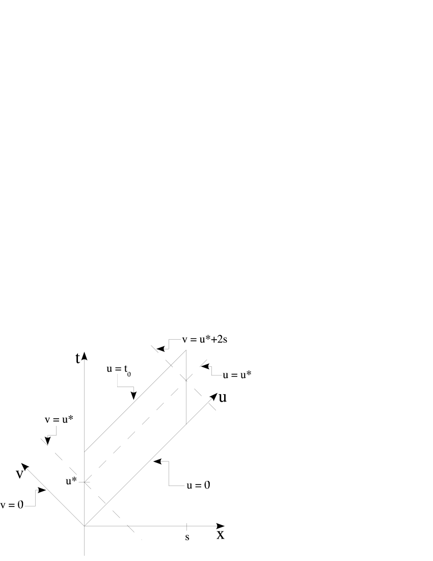
Figure 2: The spacetime region between the source and detector in null coordinates. For each fixed $u=u^{*}$ between $u=0$ and $u=t_{0}$, one integrates along the line $u=u^{*}$ from $v=u^{*}$ to $v=u^{*}+2s$.

The result is

$$F(\omega_{g},s,t_{0}) = \int da\int da^{\prime}\,f(x,x^{\prime})=\int_{0}^{t_{0}}du\int_{0}^{t_{0}}du^{\prime}\int_{u}^{u+2s}dv\int_{u^{\prime}}^{u^{\prime}+2s}dv^{\prime}\,f(x,x^{\prime})$$ (37)

$$= \frac{16\{1-\cos[s(\ell_{x}-\omega_{g})]\}\,[1-\cos(\omega_{g}t_{0})]}{\omega_{g}^{2}(\ell_{x}-\omega_{g})^{2}}$$

$$\times [\cosh(2r)-\sinh(2r)\cos(\theta+s\ell_{x}-\omega_{g}(t_{0}+s))-1]\,.$$

Here $s$ is the spatial separation of source and detector, and $t_{0}$ is the observation time. It should be noted that, since we integrate over a spacetime slice of constant y and z, we may set $y=y^{\prime}=z=z^{\prime}=0$. Finally, from Eq. (25), the redshift fluctuations become:

$$\delta\xi^{2}=4\,(\ell_{[\alpha}A_{\beta][\mu}\ell_{\nu]})(\ell_{[\gamma}A_{\delta][\rho}\ell_{\sigma]})t^{\alpha}k^{\beta}t^{\mu}k^{\nu}t^{\gamma}k^{\delta}t^{\rho}k^{\sigma}F(\omega_{g},s,t_{0}).$$ (38)

While from Eq. (28), the angular fluctuations are given by

$$\delta\Theta^{2}=4\,(\ell_{[\alpha}A_{\beta][\mu}\ell_{\nu]})(\ell_{[\gamma}A_{\delta][\rho}\ell_{\sigma]})s^{\alpha}k^{\beta}t^{\mu}k^{\nu}s^{\gamma}k^{\delta}t^{\rho}k^{\sigma}F(\omega_{g},s,t_{0}).$$ (39)

Interestingly, since $F(\omega_{g},s,t_{0})$ is independent of the displacement parameter, $\alpha$, so are $\delta\xi^{2}$ and $\delta\Theta^{2}$. Therefore, the fluctuations depend only on the squeezing parameter, $\zeta$, and we can immediately say that a coherent state (classical wave) for which $\zeta=0$ induces no fluctuations. For the following calculations, we assume the passing gravity waves are in the Transverse Tracefree (TT) Gauge. However, note that since our results derive from the Riemann tensor, the equations are gauge invariant, and we use the TT gauge only for calculational convenience.

To begin, note that if the gravity waves and photons travel in parallel, then one finds $(\ell_{[\alpha}A_{\beta][\mu}\ell_{\nu]})t^{\alpha}k^{\beta}t^{\mu}k^{\nu}=0$. This indicates that there is no induced redshift fluctuation nor angular blurring due to a squeezed state gravity wave traveling with the photons. This is as one might expect, since a gravity wave in the TT gauge has only non-zero transverse components. We may subsequently restrict our attention to transversely propagating gravity waves and will assume the gravity waves to propagate with $\ell^{\mu}=\omega_{g}(1,0,0,1)$ while the photons continue to have wave vector $k^{\mu}=(1,1,0,0)$. We define

$$\mathfrak{F}(\omega_{g},s,t_{0})=[1-\cos(\omega_{g}s)][1-\cos(\omega_{g}t_{0})][\cosh(2r)-\sinh(2r)\cos(\theta-\omega_{g}(t_{0}+s))-1]\,,$$ (40)

so that for a gravitational wave propagating in the z direction, for which $\ell_{x}=0$,

$$F(\omega_{g},s,t_{0})=\frac{16}{{\omega_{g}}^{4}}\mathfrak{F}(\omega_{g},s,t_{0})\,.$$ (41)

III.1.1 Redshift Fluctuations

With transversely propagating gravity waves,

$$(\ell_{[\alpha}A_{\beta][\mu}\ell_{\nu]})t^{\alpha}k^{\beta}t^{\mu}k^{\nu}=-\frac{1}{4}\omega_{g}^{2}A_{+}\,,$$ (42)

and therefore

$$\delta\xi^{2}=4\,A_{+}^{2}\mathfrak{F}(\omega_{g},s,t_{0}).$$ (43)

There exists a non-zero effect which in this case depends only on the $(+)$ polarization. For a gravity wave propagating in the $z$-direction, $A_{+}=A_{xx}=-A_{yy}$.

III.1.2 Angular Blurring

Case 1

Let the photons propagate in the x direction while the gravity waves propagate in the z direction and probe the y component of angular blurring, $s^{\mu}=(0,0,1,0)$. We find

$$(\ell_{[\alpha}A_{\beta][\mu}\ell_{\nu]})s^{\alpha}k^{\beta}t^{\mu}k^{\nu}=\frac{1}{4}\omega_{g}^{2}A_{\times}$$ (44)

and

$$\delta\Theta_{y}^{2}=4\,A_{\times}^{2}\mathfrak{F}(\omega_{g},s,t_{0}).$$ (45)

Note that here the y component of blurring depends only on the $(\times)$ polarization of the gravity waves. Here $A_{\times}=A_{xy}=A_{yx}$.

Case 2

To probe the z component of blurring, set $s^{\mu}=(0,0,0,1)$. The result is

$$\delta\Theta_{z}^{2}=4\,A_{+}^{2}\mathfrak{F}(\omega_{g},s,t_{0})\,,$$ (46)

which is the same as Eq. (43) for redshift fluctuations, and only depends on the $(+)$ polarization of the gravity waves.

III.2 Classical Time Dependent Variation

As noted above, the fluctuations in redshift and angle depend upon the degree of squeezing, measured by the parameter $\zeta$. In this subsection, we will examine the expectation value of the change in fractional redshift, $\langle\Delta\xi\rangle$ and in angle, $\langle\Delta\Theta\rangle$. These quantities will depend only upon the displacement parameter $\alpha$, and hence would be the same in the coherent state $|\alpha,0\rangle$ as they are in the squeezed state $|\alpha,\zeta\rangle$. For this reason, we regard these quantities as giving the classical time-dependence. Alternative approaches to the classical time-dependence of these quantities may be found in Refs. Weber ; Zipoy ; Kaufmann

Here it is possible to calculate $\langle\Delta\xi\rangle$ as a single integration of the Riemann tensor over the spacetime region $da$ via Eq. (17). However, for comparison purposes, we calculate $\langle\Delta\xi\rangle^{2}$ directly. In this case,

$$\langle\Delta\xi\rangle^{2}=\int da\int da^{\prime}\,\langle\hat{R}_{\alpha\beta\mu\nu}(x)\rangle\langle\hat{R}_{\gamma\delta\rho\sigma}(x^{\prime})\rangle t^{\alpha}k^{\beta}t^{\mu}k^{\nu}t^{\gamma}k^{\delta}t^{\rho}k^{\sigma}\,,$$ (47)

where now

$$\langle\hat{R}_{\alpha\beta\mu\nu}(x)\rangle\langle\hat{R}_{\gamma\delta\rho\sigma}(x^{\prime})\rangle=4\sum_{l}(\ell_{[\alpha}A_{\beta][\mu}\ell_{\nu]})(\ell_{[\gamma}A_{\delta][\rho}\ell_{\sigma]})f^{\prime}(x,x^{\prime})$$ (48)

with

$$f^{\prime}(x,x^{\prime})=\alpha^{2}e^{i\ell_{\tau}(x^{\tau}+x^{\prime\tau})}+(\alpha^{\ast})^{2}e^{-i\ell_{\tau}(x^{\tau}+x^{\prime\tau})}+2|\alpha|^{2}\cos[\ell_{\tau}(x^{\tau}-x^{\prime\tau})].$$ (49)

Integration of $f^{\prime}(x,x^{\prime})$ over the spacetime region of Fig. 1 yields

$$F^{\prime}(\omega_{g},s,t_{0})=\int da\int da^{\prime}\,f^{\prime}(x,x^{\prime})=$$

$$\frac{16\{1-\cos[s(\ell_{x}-\omega_{g})]\}[1-\cos(\omega_{g}t_{0})]}{\omega_{g}^{2}(\ell_{x}-\omega_{g})^{2}}\left(\alpha e^{\frac{i}{2}[\ell_{x}s-\omega_{g}(s+t_{0})]}+\alpha^{\ast}e^{-\frac{i}{2}[\ell_{x}s-\omega_{g}(s+t_{0})]}\right)^{2}.$$ (50)

Thus the classical time variation of the redshift is characterized by:

$$\langle\Delta\xi\rangle^{2}=4\,F^{\prime}(\omega_{g},s,t_{0})(\ell_{[\alpha}A_{\beta][\mu}\ell_{\nu]})(\ell_{[\gamma}A_{\delta][\rho}\ell_{\sigma]})t^{\alpha}k^{\beta}t^{\mu}k^{\nu}t^{\gamma}k^{\delta}t^{\rho}k^{\sigma}.$$ (51)

For the case of redshift variations with photons and a gravity wave propagating perpendicularly (Sect. III.1.1),

$$\langle\Delta\xi\rangle^{2}=4\,A_{+}^{2}\mathfrak{F^{\prime}}(\omega_{g},s,t_{0}).$$ (52)

Here $\mathfrak{F^{\prime}}(\omega_{g},s,t_{0})$ is defined in a similar way as $\mathfrak{F}(\omega_{g},s,t_{0})$ when $\ell_{x}=0$,

$$\mathfrak{F^{\prime}}(\omega_{g},s,t_{0})=[1-\cos(\omega_{g}s)][1-\cos(\omega_{g}t_{0})]\left(\alpha e^{-\frac{i\omega_{g}}{2}(s+t_{0})}+\alpha^{\ast}e^{\frac{i\omega_{g}}{2}(s+t_{0}))}\right)^{2}.$$ (53)

The classical time variation of angular position yields similar results. Particularly, for perpendicularly propagating photons and gravity waves and probing the y component of blurring (case 1 of Sect. III.1.2), one finds

$$\langle\Delta\Theta_{y}\rangle^{2}=4\,A_{\times}^{2}\mathfrak{F}^{\prime}(\omega_{g},s,t_{0}).$$ (54)

While probing the z component of blurring (case 2 of Sect. III.1.2), the result is

$$\langle\Delta\Theta_{z}\rangle^{2}=4\,A_{+}^{2}\mathfrak{F}^{\prime}(\omega_{g},s,t_{0}).$$ (55)

Note that the function $F^{\prime}(\omega_{g},s,t_{0})$, and hence $\mathfrak{F^{\prime}}(\omega_{g},s,t_{0})$, depends on the displacement parameter $\alpha$, but not on the squeeze parameter, $r$. Therefore the same can be said for results Eqs. (52), (54), and (55). In particular $\mathfrak{F^{\prime}}(\omega_{g},s,t_{0})=0$ for $\alpha=0$. This means a coherent state (classical wave), for which $r=0,\alpha\neq 0$, exhibits regular time variations but no fluctuations. Indeed, recall from Eq. (37) that $\delta\xi^{2}=\delta\Theta^{2}=0$ for $r=0$. We will exploit this fact shortly by considering a state for which $\alpha=0$.

In a time-averaged measurement, the classical time variation will produce line broadening and angular blurring, such as do the quantum spacetime fluctuations from a squeezed vacuum state. The two effects can, however, be distinguished in principle. If one were to make repeated measurements at the same point in the cycle of a gravity wave, the effects of classical time dependence would disappear, but those of quantum fluctuations would remain.

III.3 Stress Tensor for Squeezed State Gravity Waves

We would like to obtain an order of magnitude estimate for $\langle\left(\Delta\xi\right)^{2}\rangle$ and $\langle(\Delta\Theta)^{2}\rangle$. However, the gravitational wave amplitude $A_{\mu\nu}$ is not directly measurable. We therefore would like to express the previous results in terms of the energy density of the waves. While the stress-energy tensor is not well defined for a gravitational wave, one can define an effective stress tensor in the linearized theory (see, e.g., Ref. MTW ). Classically, this effective stress tensor is defined as

$$T_{\mu\nu}^{GW}=\frac{1}{32\pi}\,\langle h^{TT}_{\alpha\beta,\mu}h^{TT}_{\alpha\beta,\nu}\rangle\,.$$ (56)

Here the brackets denote a spatial average over several wavelengths and the TT superscript indicates we are working in the Transverse Tracefree gauge. We use this expression with the expectation value of a gravity wave in a squeezed state, and perform a spatial average on the quantity

$$\langle\zeta,\alpha|:\hat{h}^{TT}_{\alpha\beta,\mu}\hat{h}^{TT}_{\alpha\beta,\nu}:|\alpha,\zeta\rangle$$ (57)

This operation results in an effective stress tensor of the form

$$T_{\mu\nu}=\frac{1}{32\pi}\,\sum_{\alpha,\beta}A_{\alpha\beta}^{2}k_{\mu}k_{\nu}[2|\alpha|^{2}+\cosh(2r)]$$ (58)

while

$$:T_{\mu\nu}:\,=\frac{1}{32\pi}\,\sum_{\alpha,\beta}A_{\alpha\beta}^{2}k_{\mu}k_{\nu}[2|\alpha|^{2}+\cosh(2r)-1].$$ (59)

The vacuum energy term, $T_{00}^{vac}=T_{00}-:T_{00}:$ is then

$$T_{00}^{vac}=\frac{1}{32\pi}\,\sum_{\alpha,\beta}A_{\alpha\beta}^{2}\omega_{g}^{2}\,.$$ (60)

Examining the contribution from the $(+)$ polarization, where $A_{+}=A_{xx}=-A_{yy}$ and $A_{\times}=A_{xy}=A_{yx}=0$, one finds

$$T_{00}^{vac}=\frac{1}{16\pi}\,A_{+}^{2}\omega_{g}^{2}.$$ (61)

However, since the quantum vacuum energy is also $\frac{1}{2}\omega_{g}$, we can use the vacuum mode to fix the normalization.

$$VT_{00}^{vac}=\frac{1}{16\pi}\,A_{+}^{2}\omega_{g}^{2}V=\frac{1}{2}\omega_{g}$$ (62)

for each $\bm{\ell}$, where $V$ is the quantization volume, which leads to

$$A_{+}=\sqrt{\frac{8\pi}{\omega_{g}V}}.$$ (63)

For the $(\times)$ polarization, one also finds

$$A_{\times}=\sqrt{\frac{8\pi}{\omega_{g}V}}.$$ (64)

The previous results, Eqs. (43), (45), and (46) become

$$\delta\xi^{2}=\delta\Theta_{y}^{2}=\delta\Theta_{z}^{2}=\frac{32\pi}{\omega_{g}V}\,\mathfrak{F}(\omega_{g},s,t_{0})\,.$$ (65)

So far, we have considered a single mode. However, we may also have a situation in which many modes are excited. In this case, we would insert a sum on modes on the right hand side of the above equation. If the density of states is large, we let

$$\sum_{\ell}\rightarrow\frac{V}{(2\pi)^{3}}\int{d^{3}\bm{\ell}}.$$ (66)

Suppose the distribution of gravity waves in $\bm{\ell}$-space is narrowly peaked about some $\omega_{g}$ with characteristic width $\Delta\omega_{g}$. If $\Delta\omega_{g}$ is small, then the integrand is essentially constant over the region of integration. The result of the integration is just the integrand multiplied by a volume, $(\Delta\ell_{x})(\Delta\ell_{y})(\Delta\ell_{z})$, in $\bm{\ell}$-space, with $\Delta\ell_{i}$ a bandwidth in the $i$-direction of $\bm{\ell}$-space. Specifically,

$$\delta\xi^{2}=\frac{\omega_{g}^{3}}{4\pi^{2}}\,(\Delta\ell_{x})(\Delta\ell_{y})(\Delta\ell_{z})\,F(\omega_{g},s,t_{0}).$$ (67)

III.4 Estimate of $\delta\xi^{2}$ and $\delta\Theta^{2}$

Recall that from Eqs. (52), (54), and (55), the classical time variation depends on the displacement parameter, $\alpha$, but not on the squeeze parameter $\zeta$. For the purpose of obtaining order of magnitude estimates of $\delta\xi^{2}$ and $\delta\Theta^{2}$, suppose $\alpha=0$ and $r\gg 1$; further assume the $+$ polarization, so that $A_{\times}=0$. Since for $\alpha=0$, $\mathfrak{F^{\prime}}(\omega_{g},s,t_{0})=0$, it is clear that $\langle\Delta\xi\rangle^{2}=0$ and $\langle\Delta\Theta\rangle^{2}=0$, from Eqs. (52) and (55), respectively. Therefore, for the case $\alpha=0$ one finds $\delta\xi^{2}=\langle(\Delta\xi)^{2}\rangle$ and $\delta\Theta^{2}=\langle(\Delta\Theta)^{2}\rangle$.

Using Eqs. (59) and (63), and integrating over a sharply peaked distribution function in $\bm{\ell}$-space, the energy density for large $r$ becomes

$$:T_{00}:\,\approx\frac{\omega_{g}e^{2r}}{4(2\pi)^{3}}\Delta\ell_{x}\Delta\ell_{y}\Delta\ell_{z}.$$ (68)

From Eqs. (37) and (67), we have for large $r$,

$$\langle(\Delta\xi)^{2}\rangle\approx\frac{2\,e^{2r}}{\pi^{2}\omega_{g}}\Delta\ell_{x}\Delta\ell_{y}\Delta\ell_{z}.$$ (69)

Thus

$$\langle(\Delta\xi)^{2}\rangle\approx 64\pi\frac{:T_{00}:}{\omega_{g}^{2}}=64\pi\frac{:T_{00}:}{\omega_{g}^{2}}\ell_{\rm Pl}^{2}\,,$$ (70)

where $\ell_{\rm Pl}$ is the Planck length. With $\omega_{g}=2\pi/\lambda_{g}$, we have

$$\langle(\Delta\xi)^{2}\rangle\approx\frac{16}{\pi}\ell_{\rm Pl}^{2}\lambda_{g}^{2}:T_{00}:\quad\mbox{or}\quad(\Delta\xi)_{rms}\approx\ell_{\rm Pl}\lambda_{g}\sqrt{:T_{00}:}\,.$$ (71)

Suppose for example a gravity wave with $\lambda_{g}=1\,\mbox{ly}=10^{18}\mbox{cm}$ and the closure energy density $:T_{00}:\,=10^{8}\mbox{cm}^{-4}$. Then with $\ell_{\rm Pl}=10^{-33}\mbox{cm}$,

$$(\Delta\xi)_{rms}\approx 10^{-33}10^{18}\sqrt{10^{8}}=10^{-11}\,.$$ (72)

By comparing Eqs. (43) and (46), the order of magnitude of $(\Delta\Theta)_{rms}$ will be the same as the result for $(\Delta\xi)_{rms}$.

In principle, the effect can be made as large as desired by increasing the squeezing parameter $r$, which increases the energy density of the wave. However, as shown from the estimate given, this is a very small effect and is likely to be unobservable in the present day universe. This example serves as a useful model for spacetime geometry fluctuations, which will have large effects in the early universe and in the vicinity of black holes.

IV Thermal Bath of Gravitons

In the previous section, the fluctuation effects of a gravitational wave in a single mode squeezed state were examined. Another useful example is a thermal bath of gravitons, such as might be created by an evaporating black hole. We now consider such a thermal bath as the source of spacetime fluctuations. In particular, suppose the spacetime geometry fluctuates in such a way that $\langle\Gamma_{\alpha\beta}^{\mu}\rangle=\langle R^{\mu}_{\phantom{\mu}\alpha\nu\beta}\rangle=0$, but $\langle R^{\mu}_{\phantom{\mu}\alpha\nu\beta}R^{\gamma}_{\phantom{\gamma}\delta\rho\sigma}\rangle_{\beta}\neq 0$. In effect, we are ignoring the average spacetime curvature due to the bath of gravitons. In this case the Riemann tensor correlation function is

$$C_{\alpha\beta\mu\nu\,\gamma\delta\rho\sigma}(x,x^{\prime})=\langle R_{\alpha\beta\mu\nu}(x)R_{\gamma\delta\rho\sigma}(x^{\prime})\rangle_{\beta}\,,$$ (73)

and therefore

$$\delta\xi^{2}=\langle(\Delta\xi)^{2}\rangle=\int da\int da^{\prime}\,\langle R_{\alpha\beta\mu\nu}(x)R_{\gamma\delta\rho\sigma}(x^{\prime})\rangle_{\beta}\,t^{\alpha}k^{\beta}t^{\mu}k^{\nu}t^{\gamma}k^{\delta}t^{\rho}k^{\sigma}$$ (74)

and

$$\delta\Theta^{2}=\langle(\Delta\Theta)^{2}\rangle=\int da\int da^{\prime}\,\langle R_{\alpha\beta\mu\nu}(x)R_{\gamma\delta\rho\sigma}(x^{\prime})\rangle_{\beta}\,s^{\alpha}k^{\beta}t^{\mu}k^{\nu}s^{\gamma}k^{\delta}t^{\rho}k^{\sigma}\,,$$ (75)

where $\langle R_{\alpha\beta\mu\nu}(x)R_{\gamma\delta\rho\sigma}(x^{\prime})\rangle_{\beta}$ is the thermal normal-ordered Riemann tensor two point function.

IV.1 Redshift Fluctuations

In the average rest frame of the source and detector, let $v^{\mu}=t^{\mu}=(1,0,0,0)$ and $k^{\mu}=(1,1,0,0)$ as previously. With this and the symmetry and cyclic properties of the Riemann tensor, Eq. (74) reduces to

$$\langle(\Delta\xi)^{2}\rangle=\int da\int da^{\prime}\,\langle R_{0101}(x)R_{0101}(x^{\prime})\rangle_{\beta}.$$ (76)

We construct the thermal Riemann tensor two point function via the Matsubara method as an infinite image sum in imaginary time of the vacuum two point function. We proceed for the moment in the Feynman gauge, but since we are strictly dealing with functions of the Riemann tensor, the result will be gauge independent. From Eq. (30) and the symmetry properties of the metric tensor, the Riemann tensor vacuum two-point function can be written as

$$\langle R_{0101}(x)R_{0101}(x^{\prime})\rangle\\ =\frac{1}{4}\langle(2h_{01,01}-h_{00,11}-h_{11,00})(x)(2h_{01,01}-h_{00,11}-h_{11,00})(x^{\prime})\rangle\\ =\frac{1}{4}[4G_{0101,0101}-2G_{0100,0111}-2G_{0111,0100}-2G_{0001,1101}+G_{0000,1111}\\ +G_{0011,1100}-2G_{1101,0001}+G_{1100,0011}+G_{1111,0000}].$$ (77)

Here, $G_{\alpha\beta\mu\nu}$ is the metric two point function. The first two indices on $G_{\alpha\beta\mu\nu}$ refer to point $x$ while the second two refer to point $x^{\prime}$ and similarly for the derivative indices. In the Feynman gauge

$$G_{\alpha\beta\mu\nu}=(\eta_{\alpha\mu}\eta_{\beta\nu}+\eta_{\alpha\nu}\eta_{\beta\mu}-\eta_{\alpha\beta}\eta_{\mu\nu})D$$ (78)

where $D$ is the vacuum scalar two point function

$$D=\frac{1}{4\pi^{2}}\frac{1}{(\Delta\vec{x})^{2}-(\Delta t)^{2}}\,.$$ (79)

One finds that the only nonzero components of $G_{\alpha\beta\mu\nu}$ are $G_{0101},G_{0000},G_{0011},G_{1100}$, and $G_{1111}$ and thus

$$\langle R_{0101}(x)R_{0101}(x^{\prime})\rangle=\\ \frac{1}{4}[-4D,_{txt^{\prime}x^{\prime}}+D,_{xxx^{\prime}x^{\prime}}+D,_{xxt^{\prime}t^{\prime}}+D,_{ttx^{\prime}x^{\prime}}+D,_{ttt^{\prime}t^{\prime}}].$$ (80)

One can easily see from the function $D$ that $D,_{txt^{\prime}x^{\prime}}=D,_{xxt^{\prime}t^{\prime}}=D,_{ttx^{\prime}x^{\prime}}=\partial_{t}^{2}\partial_{x}^{2}D$ and therefore

$$\langle R_{0101}(x)R_{0101}(x^{\prime})\rangle=\frac{1}{4}(\partial_{t}^{4}-2\partial_{t}^{2}\partial_{x}^{2}+\partial_{x}^{4})D.$$ (81)

It is now clear that the thermal Riemann tensor two point function may be constructed from the vacuum two point function by making the replacement $D\rightarrow D_{\beta}$ whence

$$\langle R_{0101}(x)R_{0101}(x^{\prime})\rangle_{\beta}=\frac{1}{4}(\partial_{t}^{4}-2\partial_{t}^{2}\partial_{x}^{2}+\partial_{x}^{4})D_{\beta}.$$ (82)

As mentioned earlier, $D_{\beta}$ is constructed via the Matsubara method. First make $D$ periodic in imaginary time and then take an infinite image sum so that

$$D_{\beta}=\frac{1}{4\pi^{2}}\sideset{}{{}^{\prime}}{\sum}_{n=-\infty}^{\infty}\frac{1}{(\Delta\vec{x})^{2}-(t-t^{\prime}+in\beta)^{2}}.$$ (83)

The prime on the summation indicates that we leave out the $n=0$ term, which corresponds to the vacuum term. As a result, Eq. (82) gives a normal-ordered two-point function. We can set $y-y^{\prime}=z-z^{\prime}=0$, and use null coordinates to write

$$D_{\beta}=\frac{1}{4\pi^{2}}\sideset{}{{}^{\prime}}{\sum}_{n=-\infty}^{\infty}\frac{1}{n^{2}\beta^{2}-\Delta v\Delta u-in\beta(\Delta v+\Delta u)}.$$ (84)

This, with the null coordinate version of Eq. (82), gives

$$\langle(\Delta\xi)^{2}\rangle=4\int da\int da^{\prime}\,\partial_{u}\partial_{u^{\prime}}\partial_{v}\partial_{v^{\prime}}D_{\beta}.$$ (85)

The integral can be evaluated in the following way. First note that we are interested in the real part of $D_{\beta}$, which is even in $n$, so that we may make the replacement

$$\sideset{}{{}^{\prime}}{\sum}_{n=-\infty}^{\infty}\rightarrow 2\sum_{n=1}^{\infty}$$

and let

$$Re(D_{\beta})=\frac{1}{2\pi^{2}}\sum_{n=1}^{\infty}G$$ (86)

where

$$G=Re\left[\frac{1}{n^{2}\beta^{2}-\Delta v\Delta u-in\beta(\Delta v+\Delta u)}\right].$$ (87)

In null coordinates,

$$\langle(\Delta\xi)^{2}\rangle=\frac{2}{\pi^{2}}\sum_{n=1}^{\infty}\int_{0}^{t_{0}}du\int_{0}^{t_{0}}du^{\prime}\int_{u}^{u+2s}dv\int_{u^{\prime}}^{u^{\prime}+2s}dv^{\prime}\,\partial_{v}\partial_{v^{\prime}}\partial_{u}\partial_{u^{\prime}}G.$$ (88)

Performing the integrations on $v$ and $v^{\prime}$ yields

$$\langle(\Delta\xi)^{2}\rangle=\frac{2}{\pi^{2}}\sum_{n=1}^{\infty}\int_{0}^{t_{0}}du\int_{0}^{t_{0}}du^{\prime}\,I(\Delta u)\,,$$ (89)

where we make use of the fact that $\partial_{u}\partial_{u^{\prime}}G=-\partial_{u}^{2}G$ in writing

$$I(\Delta u)=(\partial_{u}^{2}G)\Bigr{|}_{\Delta v=\Delta u+2s}+(\partial_{u}^{2}G)\Bigr{|}_{\Delta v=\Delta u-2s}-2(\partial_{u}^{2}G)\Bigr{|}_{\Delta v=\Delta u}.$$ (90)

The function $I(\Delta u)$ is a function of $\Delta u$ only, for which

$$\int_{0}^{t_{0}}du\int_{0}^{t_{0}}du^{\prime}\,I(\Delta u)=\int_{0}^{t_{0}}d(\Delta u)(t_{0}-\Delta u)I(\Delta u)+\int_{-t_{0}}^{0}d(\Delta u)(t_{0}+\Delta u)I(\Delta u).$$ (91)

This now leads to the expression

$$\langle(\Delta\xi)^{2}\rangle=\frac{2}{\pi^{2}}\sum_{n=1}^{\infty}\int_{0}^{t_{0}}d(\Delta u)(t_{0}-\Delta u)I(\Delta u)+\int_{-t_{0}}^{0}d(\Delta u)(t_{0}+\Delta u)I(\Delta u).$$ (92)

Equation (92) can be evaluated using a program such as Maple. The complete result is a rather lengthy expression and no insight is gained by writing it out. However, in the limit where $s\gg t_{0}$ and $s\gg\beta$, i.e., the observationally reasonable limit where the distance between source and detector is much larger than both the observation time and the thermal wavelength, the expression reduces to

$$\langle(\Delta\xi)^{2}\rangle\sim\frac{4}{9\pi^{2}a^{2}\beta^{2}}[3\pi^{2}a^{2}\mbox{csch}^{2}(\pi a)+\pi^{2}a^{2}-3],$$ (93)

with $a={t_{0}}/{\beta}$. In the limit where the observation time is short compared to the correlation time $\beta$, i.e. $t_{0}\ll\beta$, we find

$$\langle(\Delta\xi)^{2}\rangle\sim\frac{4t_{0}^{2}\pi^{2}}{45\beta^{4}}=\frac{4t_{0}^{2}\pi^{2}\ell_{\rm Pl}^{2}}{45\beta^{4}}$$ (94)

In this case, the rms line width grows linearly with observation time,

$$(\Delta\xi)_{rms}=\frac{2\pi\ell_{\rm Pl}t_{0}}{\beta^{2}\sqrt{45}}.$$ (95)

While on the other hand if $t_{0}\gg\beta$,

$$\langle(\Delta\xi)^{2}\rangle\sim\frac{4}{9\beta^{2}}=\frac{4\ell_{\rm Pl}^{2}}{9\beta^{2}}.$$ (96)

Here the rms line width approaches a constant,

$$(\Delta\xi)_{rms}=\frac{2\ell_{\rm Pl}}{3\beta}.$$ (97)

IV.2 Angular Blurring

Turning our attention to Eq. (75), once again let $v^{\mu}=t^{\mu}=(1,0,0,0)$ and $k^{\mu}=(1,1,0,0)$; additionally let $s^{\mu}=(0,0,1,0)$. With this and the symmetry and cyclic properties of the Riemann tensor, Eq. (75) reduces to

$$\langle(\Delta\Theta)^{2}\rangle=\int da\int da^{\prime}\,\langle(R_{2101}(x)-R_{2010}(x))(R_{2101}(x^{\prime})-R_{2010}(x^{\prime}))\rangle_{\beta}.$$ (98)

Proceeding in the Feynman Gauge, the calculations follow those for redshift fluctuations. It is straightforward to show that

$$\langle(R_{yxtx}(x)-R_{ytxt}(x))(R_{yxtx}(x^{\prime})-R_{ytxt}(x^{\prime}))\rangle\\ =\frac{1}{4}(\partial_{t}^{4}+2\partial_{t}^{3}\partial_{x}-2\partial_{t}\partial_{x}^{3}-\partial_{x}^{4})D=-4\partial_{u}\partial_{v}^{2}\partial_{v^{\prime}}D\,.$$ (99)

In null coordinates, the equation for angular blurring becomes

$$\langle(\Delta\Theta)^{2}\rangle=-4\int_{0}^{t_{0}}du\int_{0}^{t_{0}}du^{\prime}\int_{u}^{u+2s}dv\int_{u^{\prime}}^{u^{\prime}+2s}dv^{\prime}\,\partial_{u}\partial_{v}^{2}\partial_{v^{\prime}}D.$$ (100)

This integral can be solved via the same method invoked in the previous subsection when dealing with redshift fluctuations. While it is not immediately obvious from this form of the integral, the limiting results are the same as for line broadening. Namely, in the case when $s\gg t_{0},\beta$ we again have

$$\langle(\Delta\Theta)^{2}\rangle\sim\frac{4}{9\pi^{2}a^{2}\beta^{2}}[3\pi^{2}a^{2}\mbox{csch}^{2}(\pi a)+\pi^{2}a^{2}-3],$$ (101)

In the limit where $a\rightarrow 0$, or $t_{0}\ll\beta$,

$$(\Delta\Theta)_{rms}\sim\frac{2\pi\ell_{\rm Pl}t_{0}}{\beta^{2}\sqrt{45}}\,,$$ (102)

while on the other hand when $a\rightarrow\infty$, or $t_{0}\gg\beta$,

$$(\Delta\Theta)_{rms}\sim\frac{2\ell_{\rm Pl}}{3\beta}\,.$$ (103)

As emphasized earlier, these results are independent of gauge choice. As a check, these results were also calculated in the TT gauge using the thermal two point function and Hadamard function for the TT gauge derived in Ref. Yu .

We may compare Eq. (103) with the results of Ref. Borgman , where a heuristic result is found for the angular blurring of the image of a source caused by passive fluctuations rather than active fluctuations as done here. The source of fluctuation there is taken to be thermal fluctuations in the stress tensor of a scalar field. In the high temperature limit, the passive fluctuation result is

$$(\Delta\Theta)_{pass}\sim\frac{\ell_{\rm Pl}^{2}s^{\frac{3}{2}}}{b\beta^{\frac{5}{2}}}\,,$$ (104)

where $b$ is a characteristic width of the bundle of rays. The effect is seen to increase with source-detector separation, though it should be mentioned that this result is valid for the regime $s\lesssim{\beta^{3}}/{\ell_{\rm Pl}^{2}}$. An important point is that the result for passive fluctuations has two powers of $\ell_{\rm Pl}$, while those for the active fluctuations have only one. One may therefore conclude that the effect tends to be larger for active fluctuations than for passive fluctuations.

V Summary and Discussion

In this paper, two effects of spacetime geometry fluctuation are examined. Expressions are derived for fluctuations of redshift and angular position of a source as observed by a detector. The physical manifestation of these effects is found to be a broadening of observed spectral lines and angular blurring of the image of a source. The fluctuation of these observables depends on the Riemann tensor correlation function, which in turn characterizes fluctuations in the spacetime geometry. These effects should arise for both active and passive metric fluctuations. However, in the case of passive fluctuations, it may be necessary to do some additional spacetime averaging, as was discussed in Ref. Borgman . The explicit examples discussed in the present paper concerned active fluctuations.

The effects of active spacetime fluctuations are examined by considering a linearized model of quantum gravity with gravitons occupying a squeezed vacuum state. In the absence of squeezing there is no effect, but the effects grow exponentially with the squeezing parameter and so in principle can be made quite large. The redshift and angular position fluctuations are related to the energy density of the wave, and finally an order of magnitude is estimated for a gravity wave with large energy density. The result of this estimation is quite small with questionable observability in the present day universe. The results, however, indicate this is an interesting model for investigating the properties of fluctuating spacetime geometries.

Further, a thermal bath of gravitons is considered as the source of spacetime geometry fluctuation. An expression for spectral line broadening is provided for the limit that the source-detector separation is much larger than both the observation time and the thermal wavelength. For observation times short compared to the thermal wavelength, the rms spectral line width increases linearly with the observation time. On the other hand, for observation times long compared to the thermal wavelength, the rms line width approaches a constant. The results for angular blurring mirror the results for spectral line broadening in the same limit of large source-detector separation.

Appendix A Squeezed States

A squeezed vacuum state is the natural state for a quantum mechanically created particle occupying an in-vacuum state represented in an out-Fock space. Squeezed quantum states are generated via the unitary displacement and squeeze operators. Here we provide a brief summary of the relevant ideas and results for squeezed states following primarily the notation as found in Ref. Caves ; see also Refs. Stoler ; Stoler2 ; Yuen . The displacement operator generates the set of coherent states and is defined by:

$$D(\alpha)\equiv\exp(\alpha a^{\dagger}-\alpha^{\ast}a)=e^{-\frac{|\alpha|^{2}}{2}}e^{\alpha a^{\dagger}}e^{-\alpha a},$$ (105)

where $\alpha$ is an arbitrary complex number. We will here be primarily interested in generating the coherent state $|\alpha\rangle$ by displacing the vacuum state $|0\rangle$:

$$|\alpha\rangle=D(\alpha)|0\rangle\,.$$ (106)

The displacement operator transforms $a$ and $a^{\dagger}$ as:

$$D^{\dagger}(\alpha)aD(\alpha)=a+\alpha$$ (107a)

$$D^{\dagger}(\alpha)a^{\dagger}D(\alpha)=a^{\dagger}+\alpha^{\ast}$$ (107b)

The squeeze operator is defined as

$$S(\zeta)=\exp[\frac{1}{2}\zeta^{\ast}a^{2}-\frac{1}{2}\zeta(a^{\dagger})^{2}],\quad\zeta=re^{i\theta},$$ (108)

where $\zeta$ is an arbitrary complex number. We use the convention in Caves for the squeeze operator transformations of $a$ and $a^{\dagger}$:

$$S^{\dagger}(\zeta)aS(\zeta)=a\cosh{r}-a^{\dagger}e^{i\theta}\sinh{r}$$ (109a)

$$S^{\dagger}(\zeta)a^{\dagger}S(\zeta)=a^{\dagger}\cosh{r}-ae^{-i\theta}\sinh{r}$$ (109b)

The squeezed state $|\alpha,\zeta\rangle$ is now obtained by squeezing the vacuum and then displacing it:

$$|\alpha,\zeta\rangle=D(\alpha)S(\zeta)|0\rangle.$$ (110)

References

• (1) B. L. Hu and E. Verdaguer, Living Rev. Rel. 7, 3, (2004), gr-qc/0307032.
• (2) J.W. Moffat, Phys. Rev. D 56, 6264 (1997), gr-qc/9610067.
• (3) M.T. Jaekel and S. Reynaud, Phys. Lett. A 185 143 (1994).
• (4) L.H. Ford, Phys. Rev. D 51, 1692 (1995), gr-qc/9410047
• (5) B. L. Hu and K. Shiokawa, Phys. Rev. D 57, 3474 (1998), gr-qc/9708023.
• (6) J. Ellis, N.E. Mavromatos and D.V. Nanopoulos, Gen. Rel. Grav. 32, 127 (2000), gr-qc/9904068.
• (7) Y. J. Ng and H. van Dam, Phys. Lett. B 477, 429 (2000), gr-qc/9911054.
• (8) G. Amelino-Camelia, Lect. Notes Phys. 541, 1 (2000), gr-qc/9910089.
• (9) Y. J. Ng, W. A. Christiansen and H. van Dam, Astrophys. J. 591 L87 (2003), stro-ph/0302372.
• (10) G. Amelino-Camelia, Gen. Rel. Grav. 36, 539 (2004), astro-ph/0309174.
• (11) F. Dowker, J. Henson and R. Sorkin, Mod. Phys. Lett. A 19, 1829 (2004), gr-qc/0311055.
• (12) J. Borgman and L.H. Ford, Phys. Rev. D 70 064032 (2004), gr-qc/0307043.
• (13) David M. Zipoy, Phys. Rev. 142, 825 (1966).
• (14) R.K. Sachs, A.M. Wolfe, Astrophys. J. 147 73 (1967).
• (15) W. Kaufmann, Nature 227 157 (1970).
• (16) V.B. Braginsky and M.B. Menskii, JETP Lett. 13, 417 (1971).
• (17) V.B. Braginsky, N.S. Kardashev, A.G. Polnarev and I.D. Novikov, Il Nuovo Cimento 105, 1141 (1990).
• (18) J. Weber and G. Hinds, Phys. Rev. 128, 2414 (1962).
• (19) B.S. DeWitt, Phys. Rev. 162, 1239 (1967).
• (20) L.H. Ford, Int. J. Theor. Phys. 44 1753, (2005), gr-qc/0501081.
• (21) C.W. Misner, K. Thorne and J.A. Wheeler, Gravitation, (W.H. Freeman, San Francisco, 1973)
• (22) L.P. Grishchuk and Y.V. Sidorov, Phys. Rev. 42 3413 (1990).
• (23) Hongwei Yu and L.H. Ford, Phys Rev. D 60, 084023 (1999)
• (24) Carlton M. Caves, Phys. Rev. D 23 1693 (1981)
• (25) David Stoler, Phys. Rev. D 1 3217 (1970)
• (26) David Stoler, Phys. Rev. D 4 1925 (1971)
• (27) Horace P. Yuen, Phys. Rev. A 13 2226 (1976)