BA-TH/06-530

CERN-PH-TH/2006-096

gr-qc/0601132

Massless and massive graviton spectra
in anisotropic dilatonic
brane-world cosmologies

G. De Risi

Dipartimento di Fisica, Università di Bari,
and

Istituto Nazionale di Fisica Nucleare, Sezione di Bari
Via G. Amendola 173, 70126 Bari, Italy

We consider a brane-world model in which an anisotropic brane is embedded in a dilatonic background. We find the background solutions and study the behaviour of the perturbations when the Universe evolves from an inflationary Kasner phase to a Minkowski phase. We calculate the massless mode spectrum, and find that it does not differ from that expected in standard four-dimensional cosmological models. We then evaluate the spectrum of both light (ultrarelativistic) and heavy (nonrelativistic) massive modes, and find that, at high energies, there can be a strong enhancement of the Kaluza–Klein spectral amplitude, which can become dominant in the total spectrum. The presence of the dilaton, on the contrary, decreases the relative importance of the massive modes.

1 Introduction

The brane-world scenario, developed starting from the fundamental work by Randall and Sundrum [1], has received enormous attention in the past years, mostly because it is possible to generalize it to have interesting cosmological models (see [2] for a review). The fundamental question hence is how these models can be tested, and if there are signals that could allow us to distinguish between a brane-world model and a more conventional four-dimensional cosmological one. Studying the production of cosmological perturbations during inflation is a powerful tool in trying to answer to this question. Indeed much effort was devoted in building models (see, for example [3, 4, 5, 6, 7, 8, 9, 10, 11]) so as to solve the perturbation dynamics, which is in general very hard to deal with.

In this work we develop a gravi-dilaton brane-world with a non-trivial dynamics on the brane (a lot of papers have been written generalizing the standard RS solution to a more general framework in which a scalar field is included, see for example [12, 13, 14, 15, 16, 17]. In particular, following our previous work [9], we consider a higher-dimensional $p$-brane (with $p>3$) coupled with a bulk dilaton. If we do not put matter on the brane, it is possible to solve exactly the Einstein equations to obtain a Kasner solution, with $d$ expanding and $n$ contracting dimensions, on the brane itself. The bulk equation decouples, and is solved by a warp AdS-like factor, while the dilaton grows logarithmically as it goes away from the brane.

Turning to study the dynamics of the tensor perturbations, we find that massless and massive modes can be treated independently, and do not mix. We outline a procedure that allows us to study the production of the gravitational and of the Kaluza–Klein fluctuations; we also calculate the spectral distribution of these fluctuations, amplified during an imaginary phase transition from the inflationary Kasner regime to a simple Minkowski phase. This is done for the massless mode, and for both light and heavy-massive modes with respect to the curvature scale at the transition epoch. Our results show, differently from what happens in other models present in the literature, that if the transition occurs at high enough energy, there can be a strong enhancement of the contribution of the KK modes; this should be in principle observable, since, in this regime, the complete spectrum is found to be quite different from what would be expected if there were only the conventional 4D graviton. We also find that, on the contrary, the dilaton effect results in lowering the amplitude of the KK perturbations.

The paper is organized as follows: in section 2 we present and solve the background equations. In section 3 we study the perturbation around this background, and define the action that controls the dynamics of each single mode (massless and massive) on the brane. Section 4 outlines how to develop the canonical analysis of the mode action, and how to obtain the correct canonical equation that describes the evolution of the mode during the phase transition. In section 5 we obtain the correct expression for the spectral amplitude, which is specialized for the graviton in section 6, and for the KK modes in section 7. Finally, in section 8, we make some considerations on the results obtained, and draw our conclusions.

2 Background solutions

Let us consider a model in which a brane is non-minimally coupled to a bulk dilaton $\phi$. We work in a $D$-dimensional space ($D=p+2$), and set the brane fixed at the origin: $X^{D-1}=z=0$. The action is

$$S = -\frac{M^{p}}{2}\int d^{D}x\sqrt{\left|g\right|}\left(R+2\Lambda_{D}e^{\sigma_{1}\phi}-g^{AB}\partial_{A}\phi\partial_{B}\phi\right)$$ (2.1)

$$-T_{p}\int d^{D-1}\xi\sqrt{\left|\gamma\right|}e^{(p+1)\sigma_{2}\phi},$$

where $\gamma_{AB}=g_{AB}+n_{A}n_{B}$ is the induced metric on the brane, $T_{p}$ is the brane tension, and $\Lambda_{D}$ is the bulk cosmological constant.

Variation of this action with respect to the metric and to the dilaton gives the Einstein equations:

$$G_{AB}=\left[\Lambda_{D}e^{\sigma_{1}\phi}-\frac{1}{2}\left(\partial_{c}\phi\right)^{2}\right]g_{AB}+\partial_{A}\phi\partial_{B}\phi+\sqrt{\frac{|\gamma|}{|g|}}\frac{T_{p}}{M^{p}}e^{(p+1)\sigma_{2}\phi}\gamma_{AB}~{}\delta(z),$$ (2.2)

and the dilaton equation:

$$\partial_{A}\partial^{A}\phi+\sigma_{1}\Lambda_{D}e^{\sigma_{1}\phi}+(p+1)\sigma_{2}\sqrt{\frac{|\gamma|}{|g|}}\frac{T_{p}}{M^{p}}e^{(p+1)\sigma_{2}\phi}~{}\delta(z).$$ (2.3)

These equations, written as above, already include the Israel junction conditions [18], which can be deduced by integrating along a small interval across the brane on a geodesic perpendicular to the brane itself [19, 2] (see also [20]). They read, for the Einstein equations (2.2)

$$\left[k_{AB}\right]=-\frac{1}{p}\frac{T_{p}}{M^{p}}\left(e^{(p+1)\sigma_{2}\phi}\gamma_{AB}\right),$$ (2.4)

where the square brackets denote the difference between the left and the right limiting value on the brane:

$$\left[f\right]=\left(\lim_{\epsilon\rightarrow 0^{+}}-\lim_{\epsilon\rightarrow 0^{-}}\right)f(\epsilon),$$ (2.5)

and $k_{AB}$ is the extrinsic curvature on the brane.

To solve the equations we set the following ansatz on the metric:

$$ds^{2}=f^{2}(z)\left(dt^{2}-a^{2}(t){\bf dx^{2}}-b^{2}(t){\bf dy^{2}}-dz^{2}\right),$$ (2.6)

i.e. we allow the metric to be anisotropic, and impose that $d$ spatial dimensions expand and the other $n$ contract $(p=d+n)$. We also impose that the dilaton depend only on the extra-dimension: $\phi=\phi(z)$. The equations specialize in:

$$-pF^{\prime}-\frac{p(p-1)}{2}F^{2}+\frac{d(d-1)1}{2}H^{2}+\frac{n(n-1)1}{2}G^{2}+dnHG$$

$$=\frac{1}{2}\phi^{\prime 2}+\Lambda_{D}e^{\sigma_{1}\phi}f^{2}$$ (2.7)

$$-pF^{\prime}-\frac{p(p-1)}{2}F^{2}+(d-1)\dot{H}+\frac{d(d-1)}{2}H^{2}+n\dot{G}+\frac{n(n+1)}{2}G^{2}+(d-1)nHG$$

$$=\frac{1}{2}\phi^{\prime 2}+\Lambda_{D}e^{\sigma_{1}\phi}f^{2}$$ (2.8)

$$-pF^{\prime}-\frac{p(p-1)}{2}F^{2}+d\dot{H}+\frac{d(d+1)}{2}H^{2}+(n-1)\dot{G}+\frac{n(n-1)}{2}G^{2}+d(n-1)HG$$

$$=\frac{1}{2}\phi^{\prime 2}+\Lambda_{D}e^{\sigma_{1}\phi}f^{2}$$ (2.9)

$$-\frac{p(p+1)}{2}F^{2}+d\left(\dot{H}+\frac{d+1}{2}H^{2}\right)+n\left(\dot{G}+\frac{n+1}{2}G^{2}\right)+dnHG$$

$$=-\frac{1}{2}\phi^{\prime 2}+\Lambda_{D}e^{\sigma_{1}\phi}f^{2}$$ (2.10)

$$\phi^{\prime\prime}+pF\phi^{\prime}-\sigma_{1}\Lambda_{D}e^{\sigma_{1}\phi}f^{2}=0,$$ (2.11)

where dots (primes) denote differentiation w.r.t. $t$ ($z$), and $H=\dot{a}/a$, $G=\dot{b}/b$, $F=f^{\prime}/f$. Note that the singular part is absent from the above equations, because it will be taken into account by satisfying the Israel junction conditions. Inserting the ansatz (2.6) into (2.4) we get the metric junction condition:

$$\left[f^{\prime}\right]=-\frac{1}{p}\frac{T_{p}}{M^{p}}\left.\left(e^{(p+1)\sigma_{2}\phi}f^{2}\right)\right|_{z=0}.$$ (2.12)

The dilaton junction condition is obtained directly by applying on eq. (2.3) the integration procedure described above, as in standard one-dimensional quantum mechanics, and it reads

$$\left[\phi^{\prime}\right]=(p+1)\sigma_{2}\frac{T_{p}}{M^{p}}\left.\left(e^{(p+1)\sigma_{2}\phi}f\right)\right|_{z=0}.$$ (2.13)

The Einstein equations (2.7–2.10) can be decoupled, and the time dependence is solved, as in [9], by the Kasner solution:

$$a(t)=\left|\frac{t}{t_{0}}\right|^{\lambda}\, b(t)=\left|\frac{t}{t_{0}}\right|^{\mu}\$$

$$\lambda=\frac{1\pm\sqrt{\frac{n(d+n-1)}{d}}}{d+n}\, \mu=\frac{1\mp\sqrt{\frac{d(d+n-1)}{n}}}{d+n},$$ (2.14)

which can describe a superinflationary solution [21, 22] on the negative branch of the time axis, if we choose the minus sign in $\lambda$ and allow for 2 or more internal dimensions (of course, in the framework of superstring theory there is room for up to 5 internal compact dimensions if we want 3 external and one warped). So we are left with the $z$ dependent part of the Einstein equations, which can be rearranged as:

$$-pF^{\prime}-p^{2}F^{2} = 2\Lambda_{D}e^{\sigma_{1}\phi}f^{2}$$

$$-pF^{\prime}+pF^{2} = \phi^{\prime 2},$$ (2.15)

and the dilaton equation (2.11), which nevertheless depends on the other equations by means of the Bianchi identities, as expected.

To solve eqs. (2.15) we seek for a solution of the form [23, 14]:

$$f(z) = \left(1+\frac{z}{z_{0}}\right)^{\alpha}$$

$$\phi(z) = \log\left(1+\frac{z}{z_{0}}\right)^{\beta};$$ (2.16)

here $z_{0}$ is a positive constant (which corresponds to the AdS length in the usual RS model), and the solutions are intended to be in the $z>0$ region, since we consider a $Z_{2}$ symmetric background. By inserting these expressions in (2.15) and taking into account the Israel junction conditions (2.12) and (2.13) we get the following expressions for the exponents

$$\alpha=\frac{4}{p\sigma_{1}^{2}-4},~{}~{}~{}~{}~{}~{}\beta=-\frac{2p\sigma_{1}}{p\sigma_{1}^{2}-4},$$ (2.17)

and the following relations between the parameters

$$\sigma_{2} = \frac{\sigma_{1}}{2(p+1)}$$

$$\frac{T_{p}}{M^{p}} = \frac{8p}{z_{0}(4-p\sigma_{1}^{2})}$$

$$\Lambda_{D} = -2\frac{4p(p+1)-p^{2}\sigma_{1}^{2}}{(z_{0}(4-p\sigma_{1}^{2}))^{2}}.$$ (2.18)

To get a positive brane tension and a negative bulk cosmological constant, we assume that:

$$-\frac{2}{\sqrt{p}}<\sigma_{1}<\frac{2}{\sqrt{p}}.$$ (2.19)

From (2.18) it is easy to get the relation between the brane tension and the bulk cosmological constant

$$\frac{T_{p}}{M^{p}}=4\sqrt{\frac{-2\Lambda_{D}}{4\frac{p+1}{p}-\sigma_{1}^{2}}},$$ (2.20)

which is the generalization of the fine-tuning relation in the standard RS scenario.

It is possible to obtain a different class of solutions, by imposing a different ansatz:

$$f(z) = e^{-\alpha z/z_{0}}$$

$$\phi(z) = -\beta\frac{z}{z_{0}}.$$ (2.21)

This solution saturates the bound (2.19) $\sigma_{1}=2/\sqrt{p}$, and has the exponents related as follows

$$\beta=\pm\sqrt{p}\alpha.$$ (2.22)

The relation between the tension and the cosmological constant is unchanged

$$\frac{T_{p}}{M^{p}}=\sqrt{-8\Lambda_{D}}.$$ (2.23)

Nevertheless, we will only consider in what follows the first kind of solution described above.

3 Perturbation equations

In this section we are going to derive the equations of motion for the tensor perturbations of the metric, $\delta^{(1)}g_{AB}=h_{AB}$. We set the dilaton perturbation equal to zero, $\delta^{(1)}\phi=0$, because it would decouple from the tensor fluctuations, impose that the perturbation depends on only the external spatial dimensions and work in the transverse-traceless gauge:

$$h_{0A}=h_{aA}=h_{D-1,A}=0,~{}~{}~{}~{}~{}~{}g^{ij}h_{ij}=\nabla_{j}h_{i}^{~{}j}=0.$$ (3.1)

The second-order perturbation of the countervariant indices of the metric and of the dilaton is set to zero as well. To obtain the expression of the induced metric, we use the equation

$$g_{AB}n^{A}n^{B}=-1=\left(g^{(0)}_{AB}+h_{AB}\right)\left(n^{(0)A}+\delta^{(1)}n^{A}\right)\left(n^{(0)B}+\delta^{(1)}n^{B}\right).$$ (3.2)

The zeroth-order part of this expression is equal to $-1$, and we can ignore orders higher than the first. Then eq. (3.2) becomes:

$$2g_{AB}n^{(0)A}\delta^{(1)}n^{B}=0=-\frac{1}{f}\delta^{(1)}n^{5}.$$ (3.3)

So the extra-dimensional part of the normal unit vector vanishes, and therefore the complete vector is left unchanged as well, $\delta^{(1)}n^{A}=0$. This shows that the induced perturbed metric is:

$$\delta^{(1)}\gamma_{AB}\equiv\bar{h}_{AB}=\left.h_{AB}\right|_{z=0}.$$ (3.4)

The perturbation equations can be obtained by variating the action (2.1) perturbed to order $h^{2}$. After some algebraic manipulation and making use of the background equations (2.7–2.10), we find the final form:

$$\delta^{(2)}S_{(a)}=\frac{M^{d}}{4}\int d^{d+1}xdz~{}a^{d}b^{n}f^{p}\left[\dot{h}_{(a)}^{2}-\sum_{k=1}^{d}\frac{(\partial_{k}h_{(a)})^{2}}{a^{2}}-h_{(a)}^{\prime 2}\right],$$ (3.5)

where we have assumed that the internal dimensions have been compactified on a compact manifold of size $M^{-n}$. This is the action for the single polarization mode: $\delta^{(2)}S=\sum_{(a)}\delta^{(2)}S_{(a)}$. The polarization mode $h_{(a)}$ is defined via the spin-2 polarization tensors, $h_{ij}=h_{(a)}\epsilon^{(a)}_{ij}$, which satisfy the relation: $\epsilon_{~{}k}^{l~{}(a)}\epsilon_{~{}l}^{k~{}(b)}=2\delta^{ab}$. From now on we will omit the polarization index $a$. Variation of (3.5) leads to the equation of motion for each mode of the tensor perturbations, which is, as expected, the $D$-dimensional covariant d’Alembert operator on the background considered:

$$\ddot{h}+\left(dH+nG\right)\dot{h}-\frac{\nabla^{2}}{a^{2}}h-h^{\prime\prime}-pFh^{\prime}=0.$$ (3.6)

We now need a prescription to project the perturbation equations, which is free of singularities, on the brane. This condition can be obtained by perturbing to the first order the Israel junction condition (2.4). Making use of the particular form of the metric (2.6) we derive the condition:

$$\left.\left(-\frac{1}{p}\frac{T_{p}}{M^{p}}e^{(p+1)\sigma_{2}\phi}h\right)\right|_{z=0}=\left.\left(\frac{1}{f}\left(h^{\prime}+2Fh\right)\right)\right|_{z=0}.$$ (3.7)

To solve the perturbation equation (3.6), we can expand its solutions on an orthogonal basis of functions of $z$ (the precise form of the scalar product, and consequently of the normalization of the functions, will be discussed shortly):

$$h(t,x^{i},z)=v_{0}(t,x^{i})\psi_{0}(z)+\int dm~{}v_{m}(t,x^{i})\psi_{m}(z)=h_{0}+\int dm~{}h_{m}.$$ (3.8)

Inserting this expansion in (3.6) and in (3.7) leads respectively to the two equations (which are valid for both the massless and the massive modes):

$$\psi^{\prime\prime}_{m}+pF\psi^{\prime}_{m}=-m^{2}\psi_{m}$$ (3.9)

$$\ddot{v}_{m}+\left(dH+nG\right)\dot{v}_{m}-\frac{\nabla^{2}}{a^{2}}v_{m}=-m^{2}v_{m},$$ (3.10)

and to the condition

$$\int dm~{}v_{m}\left.\left[\frac{1}{f}\left(\psi^{\prime}_{m}+2F\psi_{m}\right)+\frac{1}{p}\frac{T_{p}}{M^{p}}e^{(p+1)\sigma_{2}\phi}\psi_{m}\right]\right|_{z=0}=0.$$ (3.11)

Let us now substitute the decomposition (3.8) into the action (3.5). First we consider the zero mode. After integrating by parts and making use of (3.9) we get

$$\delta^{(2)}S_{0}=\frac{M^{d}}{4}\int dz~{}f^{p}|\psi_{0}|^{2}\int d^{d+1}x~{}a^{d}b^{n}\left[\dot{v}_{0}^{2}-\sum_{i=1}^{d}\frac{(\partial_{i}v_{0})^{2}}{a^{2}}\right].$$ (3.12)

So it is clear that the auxiliary field $\hat{\psi}_{0}=\sqrt{M}f^{\frac{p}{2}}\psi_{0}$ has the correct canonical dimension to be normalized to unity:

$$\int dz~{}|\hat{\psi}_{0}(z)|^{2}=M\int dz~{}f^{p}|\psi_{0}(z)|^{2}=1.$$ (3.13)

From this we can write down the final form for the action that describes the evolution of the zero mode

$$\delta^{(2)}S_{0} = \frac{M^{d-1}}{4}\int d^{d+1}x~{}a^{d}(t)b^{n}(t)\left[\dot{v}_{0}^{2}-\sum_{i=1}^{d}\frac{(\partial_{i}v_{0})^{2}}{a^{2}}\right]$$ (3.14)

$$= \frac{M^{d-1}}{4|\psi_{0}(0)|^{2}}\int d^{d+1}x~{}a^{d}(t)b^{n}(t)\left[\dot{\bar{h}}_{0}^{2}-\sum_{i=1}^{d}\frac{(\partial_{i}\bar{h}_{0})^{2}}{a^{2}}\right],$$

and the effective Planck mass of the 4-dimensional effective graviton can be easily read off to be:

$$M_{\rm P}^{d-1}=\frac{M^{d-1}}{4|\psi_{0}(0)|^{2}},$$ (3.15)

as in the ordinary RS scenario [1, 9].

Now we turn to study the massive modes. Again, after a little algebraic manipulation, we arrive at

$$\delta^{(2)}S = \delta^{(2)}S_{0}+\frac{M^{d}}{4}\int dm~{}dm^{\prime}\int dz~{}f^{p}\psi_{m}\psi_{m^{\prime}}$$ (3.16)

$$\times\int d^{d+1}x~{}a^{d}b^{n}\left[\dot{v}_{m}\dot{v}_{m^{\prime}}-\sum_{i=1}^{d}\frac{(\partial_{i}v_{m}\partial_{i}v_{m^{\prime}})}{a^{2}}-m^{2}v_{m}v_{m^{\prime}}\right].$$

In this case the auxiliary fields with the correct canonical dimension are $\hat{\psi}_{m}=f^{\frac{p}{2}}\psi_{m}$, which satisfy a Schrödinger-like equation

$$\hat{\psi}^{\prime\prime}_{m}+\left[m^{2}-\left(\frac{p^{2}}{4}F^{2}+\frac{p}{2}F^{\prime}\right)\right]\hat{\psi}_{m}=0;$$ (3.17)

therefore, they can be normalized as a complete set of orthonormal solutions

$$\int_{-\infty}^{+\infty}dz~{}\hat{\psi}_{m}\hat{\psi}_{m^{\prime}}=\int dz~{}f^{p}\psi_{m}\psi_{m^{\prime}}=\delta(m-m^{\prime}).$$ (3.18)

By making use of this relation in (3.16) we finally find that the action (3.5) can be thought of as the sum of the massless mode action with an infinite set of massive actions, one for each single massive mode:

$$\delta^{(2)}S=\delta^{(2)}S_{0}+\int dm~{}\delta^{(2)}S_{m}.$$ (3.19)

The massless mode action $\delta^{(2)}S_{0}$ of (3.14) can be interpreted as the 4-dimensional graviton, while the form of the massive mode action is:

$$\delta^{(2)}S_{m}=\frac{M^{d}}{4|\psi_{m}(0)|^{2}}\int d^{d+1}x~{}a^{d}(t)b^{n}(t)\left[\dot{\bar{h}}_{m}^{2}-\sum_{i=1}^{d}\frac{(\partial_{i}\bar{h}_{m})^{2}}{a^{2}}-m^{2}\bar{h}_{m}^{2}\right].$$ (3.20)

From (3.20) we can deduce the value of the generalized “Planck mass” for each mode as the coefficient that multiplies the mode action:

$$M^{d}_{m}=\frac{M^{d}}{4|\psi_{m}(0)|^{2}}.$$ (3.21)

At this stage, two remarks are in order. The first is that the massive mode action does not contain terms that couple the massive modes to each other, i.e. each KK mode is “free” with respect to the interaction with the others. This is due to the fact that the perturbation equation (3.6) decouples (at least in the first-order approximation), so that we can treat the two equations (3.10) independently, and the Israel junction condition (3.11) can be satisfied for each massive mode independently, as we will do in section 7 (this is not true in general, see for example [10] in which a similar method leads to an action for the modes that contains coupling terms). Moreover, it is worth stressing that the massive mode action is not adimensional, since it has the dimension of a length, $[\delta^{(2)}S_{m}]=[M^{-1}]$. This is of course a consequence of the fact that the spectrum of the KK modes is continuous, and indicates that physical quantities will be obtained by integrating over a suitable mass interval. But, formally, for what concerns the manipulation to obtain the massive mode spectrum, we will treat (3.20) as a genuine canonical action. Nevertheless, the important result here is that modes do not mix and can be treated separately.

4 Canonical analysis of the perturbed action

To calculate the spectrum of the fluctuation, we need to put the actions (3.14) and (3.20) in a canonical form. In order to do this we will adopt the conformal time to describe the evolution of the system (from now on a dot will denote a derivation with respect to $\eta$):

$$d\eta=\frac{dt}{a(t)},$$ (4.1)

and introduce the pump field

$$\xi_{0}(\eta)=\sqrt{\frac{M^{d-1}}{2}}\frac{1}{\psi_{0}(0)}a^{\frac{d-1}{2}}b^{\frac{n}{2}},~{}~{}~{}~{}\xi_{m}(\eta)=\sqrt{\frac{M^{d}}{2}}\frac{1}{\psi_{m}(0)}a^{\frac{d-1}{2}}b^{\frac{n}{2}}.$$ (4.2)

Through the pump field it is possible to introduce the canonical field:

$$u_{m}(\eta,x^{i})=\xi_{m}(\eta)\bar{h}_{m}(\eta,x^{i}).$$ (4.3)

In terms of this canonical field, the action can be expressed in a normal form (valid both for $m=0$ and for $m\neq 0$):

$$\delta^{(2)}S_{m}=\frac{1}{2}\int d^{d}xd\eta~{}\left[\dot{u}_{m}^{2}-\sum_{i=1}^{d}(\partial_{i}u_{m})^{2}+\left(\frac{\ddot{\xi}_{m}}{\xi_{m}}-m^{2}a^{2}\right)u_{m}^{2}\right].$$ (4.4)

This form for the action makes it possible to adopt the standard quantization procedure: we promote $u_{m}$ to operators and impose the canonical commutation relations among the fields and their conjugate momenta $\pi_{m}(\eta,x^{i})=\dot{u}_{m}(\eta,x^{i})$:

$$\left[u_{0}(\eta,{\bf x}),u_{0}(\eta,{\bf x}^{\prime})\right]=\left[\pi_{0}(\eta,{\bf x}),\pi_{0}(\eta,{\bf x}^{\prime})\right]=0$$

$$\left[u_{m}(\eta,{\bf x}),u_{m^{\prime}}(\eta,{\bf x}^{\prime})\right]=\left[\pi_{m}(\eta,{\bf x}),\pi_{m^{\prime}}(\eta,{\bf x}^{\prime})\right]=0$$

$$\left[u_{0}(\eta,{\bf x}),\pi_{0}(\eta,{\bf x}^{\prime})\right]=i\delta^{d}({\bf x}^{\prime}-{\bf x})$$

$$\left[u_{m}(\eta,{\bf x}),\pi_{m^{\prime}}(\eta,{\bf x}^{\prime})\right]=i\delta(m-m^{\prime})\delta^{d}({\bf x}-{\bf x}^{\prime});$$ (4.5)

we then express them in terms of their Fourier components:

$$u_{m}(\eta,x^{i}) = \int\frac{d^{d}k}{(2\pi)^{d/2}}\left[u_{m,k}(\eta)a_{m}(k)e^{i{\bf k}\cdot{\bf x}}+u^{*}_{m,k}(\eta)a^{\dagger}_{m}(k)e^{-i{\bf k}\cdot{\bf x}}\right]$$

$$\pi_{m}(\eta,x^{i}) = \int\frac{d^{d}k}{(2\pi)^{d/2}}\left[\dot{u}_{m,k}(\eta)a_{m}(k)e^{i{\bf k}\cdot{\bf x}}+\dot{u}^{*}_{m,k}(\eta)a^{\dagger}_{m}(k)e^{-i{\bf k}\cdot{\bf x}}\right].$$ (4.6)

The operators $\{a_{m}(k)\}$ can be made to obey a canonical oscillator algebra

$$\left[a_{0}({\bf k}),a_{0}({\bf k}^{\prime})\right]=\left[a^{\dagger}_{0}({\bf k}),a^{\dagger}_{0}({\bf k}^{\prime})\right]=0$$

$$\left[a_{m}({\bf k}),a_{m^{\prime}}({\bf k}^{\prime})\right]=\left[a^{\dagger}_{m}({\bf k}),a^{\dagger}_{m^{\prime}}({\bf k}^{\prime})\right]=0$$

$$\left[a_{0}({\bf k}),a^{\dagger}_{0}({\bf k}^{\prime})\right]=\delta^{d}({\bf k}-{\bf k}^{\prime})$$

$$\left[a_{m}({\bf k}),a^{\dagger}_{m^{\prime}}({\bf k}^{\prime})\right]=\delta(m-m^{\prime})\delta^{d}({\bf k}-{\bf k}^{\prime}),$$ (4.7)

and therefore they can be interpreted as a set of creation–annihilation operators, provided the wavefunctions $\{u_{m,k}(\eta)\}$ satisfy the equation (which has, again, a Schrödinger-like form):

$$\ddot{u}_{m,k}(\eta)+\omega_{m,k}^{2}(\eta)u_{m,k}(\eta)=0,$$ (4.8)

where we have denoted

$$\omega_{m,k}(\eta)=\sqrt{k^{2}+m^{2}a^{2}(\eta)-\frac{\ddot{\xi}_{m}(\eta)}{\xi_{m}(\eta)}}=\sqrt{k^{2}-V_{m,k}(\eta)},$$ (4.9)

and they are normalized according to the wronskian condition (as expected)

$$u_{m,k}(\eta)\dot{u}^{*}_{m,k}(\eta)-u^{*}_{m,k}(\eta)\dot{u}_{m,k}(\eta)=i.$$ (4.10)

We should stress that, even if the massive fields $u_{m}$ (with $m\neq 0$) do not have the correct canonical dimension, $[u_{m}]=[M^{\frac{d-2}{2}}]$, this discrepancy is compensated by the dimension of the creation–annihilation operators, as can be deduced from (4.7). So the mode coefficients $u_{m,k}$ still have the proper canonical dimension of quantum-mechanical wavefunctions: $[u_{m,k}]=[M^{-\frac{1}{2}}]$. This will be important when we will need to normalize the initial fluctuations, as we will do in the next section.

5 Derivation of the spectrum

The aim of this section is to calculate the spectral distribution for both the massless and the massive gravitational modes, using the actions developed in the last section. Hence, let us imagine a phase transition in which the Universe evolves from the inflationary regime described by the Kasner solution presented in section 2 to a simple final Minkowski era. Since we are interested in models that have 3 external dimensions, from now on we will assume $d=3$. Moreover, to have an inflationary expanding initial phase, we need, as observed before, 2 or more internal dimensions. For the sake of simplicity we will take the value $n=2$, but the consideration we will make can easily be extended to a different number of internal dimensions. The phase transition will be analysed by making use of the sudden transition approximation (see, for example, [24]), so that the geometry changes instantaneously at the conformal time $-\eta_{1}$. This approximation gives reliable results only if the frequency of the amplified modes is much lower than the transition velocity, which is estimated by the curvature scale at the end of inflation $H_{1}\sim 1/\eta_{1}a_{1}=k_{1}/a_{1}=k_{1}$ (of course $a_{1}=a(-\eta_{1})=1$). For this reason, $H_{1}$ represent a cut-off frequency.

In this framework, the Bogoliubov coefficients that describe the transformation from the $|in\rangle$ to the $|out\rangle$ states can be obtained by simply imposing continuity of the Fourier coefficients $u_{m,k}$ and their time derivative at the transition time $-\eta_{1}$. This procedure is nevertheless effective only if we have an unambiguous way to normalize the $|in\rangle$ functions to pure positive norm states. This is indeed what happens in our case, since it is easy to see that the background solutions, written in conformal time, are

$$a(\eta)=\left(-\frac{\eta}{\eta_{1}}\right)^{\bar{\lambda}}, b(\eta)=\left(-\frac{\eta}{\eta_{1}}\right)^{\bar{\mu}}$$

$$\bar{\lambda}=\frac{\lambda}{1-\lambda}, \bar{\mu}=\frac{\mu}{1-\lambda},$$ (5.1)

with the parameters $\lambda$ and $\mu$ given in (2.14); since, if we want an inflationary solution, it must be $\lambda<0$, we see that $\alpha(\eta)$ vanish as $\eta\rightarrow-\infty$. On the other side, the expression for the pump field during the Kasner regime is (note that it is independent from the number of internal and external dimensions):

$$\xi_{0}(\eta)=\sqrt{\frac{M^{d-1}}{2}}\frac{1}{\psi_{0}(0)}\sqrt{-\frac{\eta}{\eta_{1}}},~{}~{}~{}~{}~{}~{}\xi_{m}(\eta)=\sqrt{\frac{M^{d}}{2}}\frac{1}{\psi_{m}(0)}\sqrt{-\frac{\eta}{\eta_{1}}},$$ (5.2)

but of course the ratio $\ddot{\xi_{m}}/\xi_{m}$ always has the same behaviour, like $\eta^{-2}$. So the whole potential $V_{m,k}(\eta)$ goes to zero at the infinite past, and in this limit the mode equation reduces to that of a massless non-interacting field, $\ddot{u}_{m,k}+k^{2}u_{m,k}=0$. Moreover, as explained in section 4, the dimension of the mode coefficient is the same as expected, so we can guess the correct initial expression for it:

$$u_{m,k}(\eta)=\frac{1}{\sqrt{2k}}e^{-i|k|\eta}.$$ (5.3)

With this in hand, what we need to do is to find a complete solution for (4.8) fixing the free parameters in a suitable way to match the asymptotic solution (5.3), and then to solve the linear system

$$u_{m,k}^{(\rm in)}(-\eta_{1})=\alpha_{m}(k)u_{m,k}^{+(\rm out)}(-\eta_{1})+\beta_{m}(k)u_{m,k}^{-(\rm out)}(-\eta_{1})$$

$$\dot{u}_{m,k}^{(\rm in)}(-\eta_{1})=\alpha_{m}(k)\dot{u}_{m,k}^{+(\rm out)}(-\eta_{1})+\beta_{m}(k)\dot{u}_{m,k}^{-(\rm out)}(-\eta_{1}),$$ (5.4)

to find the Bogoliubov coefficient $\beta_{m}(k)$. Here $u_{m,k}^{+(\rm out)}$ and $u_{m,k}^{-(\rm out)}$ are respectively the positive- and negative-frequency eigenfunctions in the Minkowski phase. The Bogoliubov coefficient represents the amount of particles created by the gravitational fields in the mass interval $[m,m+dm]$. From this we can obtain the energy density per logarithmic interval unit for each mode:

$$\frac{d\rho_{0}(k)}{d\log k} = \frac{k^{4}}{\pi^{2}}|\beta_{0}(k)|^{2}$$ (5.5)

$$\frac{d\rho_{m}(k)}{d\log k} = \frac{k^{3}}{\pi^{2}}\sqrt{k^{2}+m^{2}}|\beta_{m}(k)|^{2}dm.$$ (5.6)

These expressions should be normalized with their respective coupling constants (3.15) and (3.21). Note that the different dimensions of the spectral distributions are balanced by the different dimensions of the massless and massive coupling constants, which explains the quantization procedure with the “odd” dimensions of section 4. Then the massive spectrum should be integrated over all masses (eventually one can be interested in the contribution of a particular mass interval). To obtain a dimensionless quantity, we then choose to normalize the spectral distributions just obtained to the scale curvature $H_{1}$ at the end of inflation. The spectral distribution can therefore be cast in its final form:

$$\Omega(k)=\Omega_{0}(k)+\Omega_{{\rm KK}}(k),$$ (5.7)

with

$$\Omega_{0}(k)=\frac{k^{4}}{\pi^{2}H_{1}^{2}M_{\rm P}^{2}}|\beta_{0}(k)|^{2}$$ (5.8)

$$\Omega_{{\rm KK}}(k)=\int dm~{}\Omega_{m}(k)=\int dm~{}\frac{k^{3}}{\pi^{2}H_{1}^{2}M_{m}^{3}}\sqrt{k^{2}+m^{2}}|\beta_{m}(k)|^{2}.$$ (5.9)

In the next sections we will apply this procedure to derive explicitly the spectral amplitudes.

6 Spectral distribution for the massless mode

The equation for the Fourier modes (4.8) becomes, in the massless case:

$$\ddot{u}_{0,k}+\left[k^{2}+\frac{1}{4\eta^{2}}\right]u_{0,k} = 0~{}~{}~{}~{}~{}~{}~{}~{}~{}~{}~{}~{}~{}\eta<-\eta_{1}$$

$$\ddot{u}_{0,k}+k^{2}u_{0,k} = 0~{}~{}~{}~{}~{}~{}~{}~{}~{}~{}~{}~{}~{}\eta>-\eta_{1},$$ (6.1)

so the $|in\rangle$, solution which asymptotically tends to (5.3), and the $|out\rangle$ solutions are:

$$u_{0,k}^{(\rm in)} = \sqrt{\frac{\pi}{4}|\eta|}H_{0}^{(2)}(k\eta)$$

$$u_{0,k}^{+(\rm out)} = \frac{e^{-ik\eta}}{\sqrt{2k}}$$

$$u_{0,k}^{-(\rm out)} = \frac{e^{ik\eta}}{\sqrt{2k}},$$ (6.2)

where $H_{0}^{(2)}$ is the Hankel function of the second kind. This gives, for the Bogoliubov coefficient $\beta$, the expression

$$\beta_{0}(k)=\sqrt{\frac{\pi}{32k\eta_{1}}}e^{ik\eta_{1}}\left[2k\eta_{1}H_{0}^{(2)}(k\eta_{1})+i\left(2H_{0}^{(2)^{\prime}}(k\eta_{1})k\eta_{1}-H_{0}^{(2)}(k\eta_{1})\right)\right].$$ (6.3)

The expression in square brackets can now be approximated for small values of the argument of the Hankel functions, since our approximation is valid if $k\eta_{1}\ll 1$, and the leading term is logarithmic. So the energy density (5.5) takes the form

$$\frac{d\rho_{0}}{d\log k}=\frac{H_{1}^{4}}{8\pi^{3}}\left(\frac{k}{k_{1}}\right)^{3}\log^{2}\frac{k}{k_{1}}.$$ (6.4)

The next step is to solve eq. (3.9) for the massless mode. Its general solution can be written as

$$\psi_{0}(z)=c_{0}+c_{1}\frac{z_{0}}{1-5\alpha}\left(1+\frac{z}{z_{0}}\right)^{1-5\alpha},$$ (6.5)

but the normalization condition (3.13) imposes $c_{1}=0$, so the only acceptable solution is the constant one $\psi_{0}(z)=c_{0}$. The free parameter $c_{0}$ can be calculated using (3.13) as well, so we get:

$$\psi_{0}=\sqrt{-\frac{1+5\alpha}{2Mz_{0}}}.$$ (6.6)

Finally, the expression for (5.8) is

$$\Omega_{0}(k)=\frac{1}{8\pi^{3}}\left(\frac{H_{1}}{M_{\rm P}}\right)^{2}\left(\frac{k}{k_{1}}\right)^{3}\log^{2}\frac{k}{k_{1}},$$ (6.7)

$$M_{\rm P}^{2}=\frac{z_{0}M^{3}}{2(-1-5\alpha)},$$ (6.8)

and it is plotted in Fig. 1 for different values of the parameters $z_{0}H_{1}$ and $\alpha$.

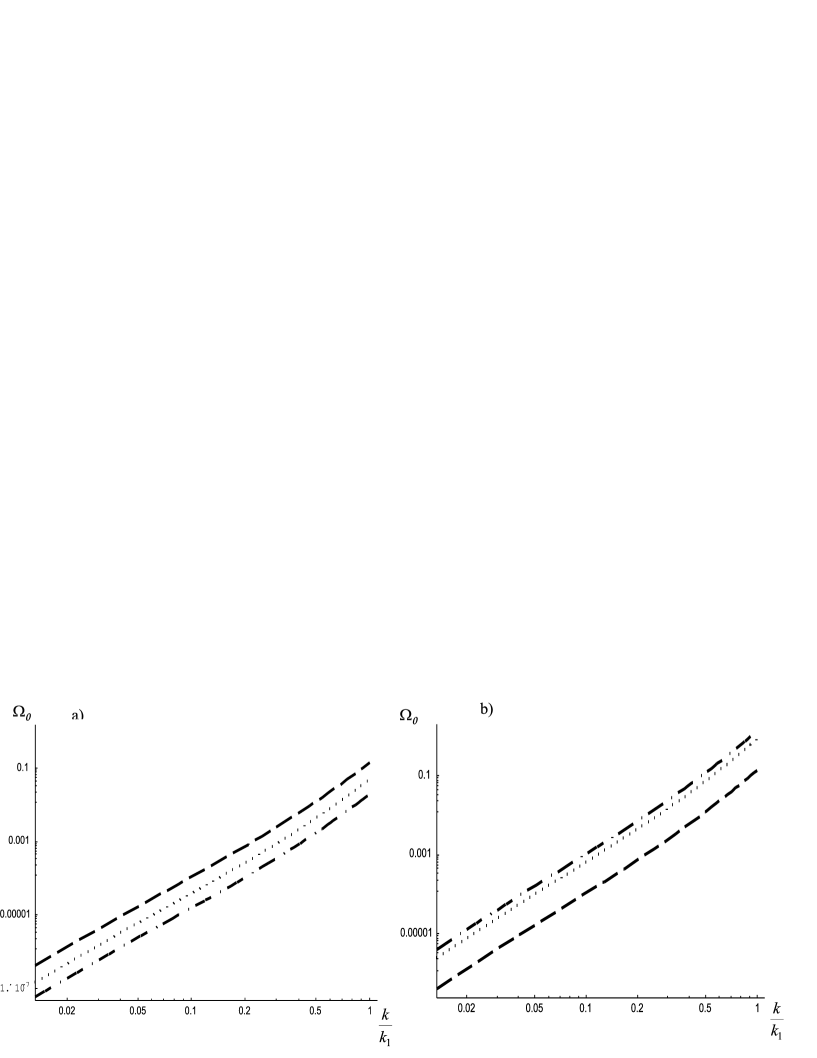
Figure 1: The spectral amplitude of the massless mode. In a) the spectrum is evaluated at $\alpha=-1$ and for $z_{0}H_{1}=7$ (dashed line), $z_{0}H_{1}=20$ (dotted line) and $z_{0}H_{1}=50$ (dot-dashed line). In b) the spectrum is evaluated at $z_{0}H_{1}=-7$ and for $\alpha=-1$ (dashed line), $\alpha=-5$ (dotted line) and $\alpha=-8$ (dot-dashed line).

7 The KK spectrum

First of all we will evaluate the massive coupling constant. In order to do this we have to solve eq. (3.17) for $m\neq 0$. Using the background solutions (2.16), it is easy to see that this equation is again a Bessel-like equation of the form:

$$\hat{\psi}^{\prime\prime}_{m}+\left(m^{2}-\frac{5\alpha(5\alpha-2)}{4}\frac{1}{(z+z_{0})^{2}}\right)\hat{\psi}_{m}=0,$$ (7.1)

and its general solution can be written as

$$\hat{\psi}_{m}(z)=\sqrt{z+z_{0}}\left[c_{1}(m)J_{\nu}(m(z+z_{0}))+c_{2}(m)Y_{\nu}(m(z+z_{0}))\right],$$ (7.2)

where $J_{\nu}$ and $Y_{\nu}$ are of course the Bessel functions of the first and of the second kind, and the parameter $\nu$ is related to the dilaton coupling constant by the relation:

$$\nu=\frac{1-5\alpha}{2}.$$ (7.3)

The constants $c_{1}$ and $c_{2}$ are fixed by using the junction condition (3.11) and the normalization condition (3.18). From the junction condition we get, using some algebraic properties of Bessel functions

$$c_{2}=-\frac{J_{\nu-1}(mz_{0})}{Y_{\nu-1}(mz_{0})}c_{1}.$$ (7.4)

From the second one, using their orthonormality relation, we get

$$c_{1}(m)=\sqrt{m}\frac{Y_{\nu-1}(mz_{0})}{\sqrt{J_{\nu-1}^{2}(mz_{0})+Y_{\nu-1}^{2}(mz_{0})}}.$$ (7.5)

Finally we can write the properly normalized solution of (7.1) as

$$\hat{\psi}_{m}(z)=\sqrt{m(z+z_{0})}\frac{\left[Y_{\nu-1}(mz_{0})J_{\nu}(m(z+z_{0}))-J_{\nu-1}(mz_{0})Y_{\nu}(m(z+z_{0}))\right]}{\sqrt{J_{\nu-1}^{2}(mz_{0})+Y_{\nu-1}^{2}(mz_{0})}}.$$ (7.6)

Now we turn to consider eq. (4.8). Actually it is very hard to solve it in its complete form, so the best we can do is to seek for particular limits in which the equation simplifies a little. As already pointed out, in the phase transition we considered, an energy scale naturally emerges, i.e. the curvature scale at the end of the inflationary epoch. In order to have a complete understanding of the effects of the KK modes, we will study what happens to lighter or heavier modes as regards to this curvature scale. Firstly, we limit our attention to modes that are lighter than the curvature scale at the end of inflation, $m\ll H_{1}$. In this case we can neglect the mass term in (4.9), so that the mode equation reduces to the same as obtained for the massless mode, eq. (6.1). It is easy to see that even if the $|out\rangle$ solutions are massive waves, the spectral distribution remains unchanged, as in eq. (6.4). So, the only contribution to the integral, which must be calculated from $m=0$ to $m=H_{1}$, comes from the massive coupling constant. The integration leads to a change of the mass parameter that controls the normalization of the spectral amplitude, while the shape of the spectrum remains unchanged. We obtain

$$\Omega_{{\rm light}}(k)=\int_{0}^{H_{1}}dm~{}\Omega_{m}(k)=\frac{1}{2\pi^{3}}\left(\frac{H_{1}}{M_{*}}\right)^{2}\left(\frac{k}{k_{1}}\right)^{3}\log^{2}\frac{k}{k_{1}},$$ (7.7)

$$M_{*}^{2}=\left(\int_{0}^{H_{1}}\frac{dm}{M_{m}^{3}}\right)^{-1}=\frac{M^{3}}{4}\left(\int_{0}^{H_{1}}dm~{}|\psi_{m}(0)|^{2}\right)^{-1}.$$ (7.8)

In Fig. 2 we show a numerical estimate of the behaviour of the spectrum for different values of the parameters.

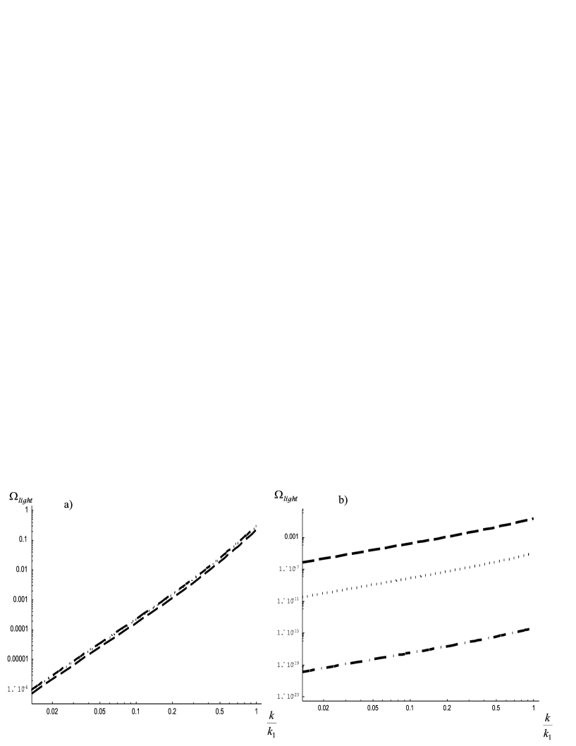
Figure 2: The spectral amplitude of light KK modes. As before, in a) the spectrum is evaluated at $\alpha=-1$ and for $z_{0}H_{1}=7$ (dashed line), $z_{0}H_{1}=20$ (dotted line) and $z_{0}H_{1}=50$ (dot-dashed line). The three curves overlap, so that they are quite confused. In b) the spectrum is evaluated at $z_{0}H_{1}=-7$ and for $\alpha=-1$ (dashed line), $\alpha=-5$ (dotted line) and $\alpha=-8$ (dot-dashed line).

Next, we try to solve (4.8) for the heavy modes. To do this, we use a WKB-like approximation for the mode function $u_{m,k}$ [25, 26], which can be written as:

$$u_{m,k}^{(in)}\simeq\frac{1}{\sqrt{2\omega_{m,k}(\eta)}}\exp\left[-i\int^{\eta}d\eta^{\prime}\omega_{m,k}(\eta^{\prime})\right].$$ (7.9)

This approximation is valid if the variation of the frequency is small with respect to the frequency itself. More precisely, (see, for example, [27]), one must have

$$\epsilon=\frac{3}{4}\frac{\dot{\omega}_{m,k}^{2}}{\omega_{m,k}^{4}}-\frac{1}{2}\frac{\ddot{\omega}_{m,k}}{\omega_{m,k}^{3}}\ll 1.$$ (7.10)

Since the parameter $\epsilon$ grows monotonically in time, we only need to check where our approximation is valid at the transition epoch $\eta_{1}$, and we are guaranteed that it always holds before that time. It is not difficult to see that $|\epsilon(-\eta_{1})|\ll 1$ if $ma_{1}\gg k_{1}$, which is exactly the regime we wish to investigate. This is not an unexpected result, since it is known [27] that this approximation works better if the transition is adiabatic, so that the variation of the curvature is slow with respect to the energy. But this means that the sudden transition approximation is no longer valid. Nevertheless, we could still get clues on the form of the spectrum by analytically continuing the function $\omega_{m,k}$ and evaluating the integral in (7.9) on a suitable path. We consider a semicircle on the upper half-plane. Its radius should be chosen to be greater than $\eta_{1}$, to stay in the region in which the WKB approximation is valid, but not too big, since we expect the mass term to be dominant with respect to the pure frequency term $k^{2}$. In this regime the function $\omega_{m,k}$ can be approximated as

$$\omega_{m,k}(\eta)\simeq ma(\eta)+\frac{k^{2}}{2ma(\eta)}-\frac{1}{2ma(\eta)}\frac{\ddot{\xi}_{m}}{\xi_{m}},$$ (7.11)

and has, as one could expect, the form of non-relativistic energy for a massive particle, plus a term that describes the direct interaction between the particle and the background geometry, which however is negligible. Note that, in the approximation (7.11), $\omega_{m,k}$ has only a singularity at the origin, so we can actually shrink the radius of the integration path till $R\simeq\eta_{1}$ without changing the result of the integration [26]. It is not difficult to see that the square modulus of the Bogoliubov coefficient is given by:

$$|\beta_{m}(k)|^{2}=\exp\left[2~{}{\rm Im}\left(\int d\eta~{}\omega_{m,k}(\eta)\right)\right].$$ (7.12)

The integral is easy to solve if we make use of the approximation (7.11), so we get:

$$|\beta_{m}(k)|^{2}=\exp\left[2\sin\pi\bar{\lambda}\left(\frac{ma_{1}}{k_{1}(1+\bar{\lambda})}-\frac{k^{2}}{2ma_{1}k_{1}(1-\bar{\lambda})}+\frac{k_{1}}{8ma_{1}(1+\bar{\lambda})}\right)\right],~{}~{}~{}~{}~{}~{}m\gg H_{1}.$$ (7.13)

This expression can now be substituted in (5.9) to obtain the final form for the Kaluza–Klein spectrum. The integral in this case runs from $m=H_{1}$ to infinity.

$$\Omega_{\rm heavy}(k)=\int_{H_{1}}^{+\infty}dm~{}\frac{k^{3}}{\pi^{2}H_{1}^{2}M_{m}^{3}}\sqrt{k^{2}+m^{2}}|\beta_{m}(k)|^{2}.$$ (7.14)

Of course this integration can only be carried out numerically. The result is presented in Fig. 3 for the same values of the parameters $z_{0}H_{1}$ and $\alpha$ used in the previous computations.

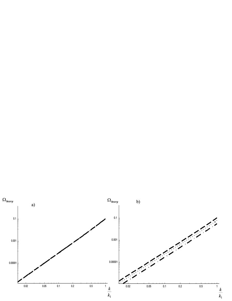
Figure 3: The spectral amplitude of the heavy KK modes. As in the other figures, plot a) represents the spectrum evaluated at $\alpha=-1$ and for $z_{0}H_{1}=7$ (dashed line), $z_{0}H_{1}=20$ (dotted line) and $z_{0}H_{1}=50$ (dot-dashed line). Again, overlapping of the curves do not permit to distinguish them. Plot b) represents the spectrum evaluated at $z_{0}H_{1}=-7$ and for $\alpha=-1$ (dashed line), $\alpha=-5$ (dotted line) and $\alpha=-8$ (dot-dashed line)

8 Comments and conclusions

In this paper we have presented a simple model in which a brane coupled with a bulk dilaton evolves from an initial inflationary Kasner phase to a final Minkowski era. Then we have studied the evolution of the tensor perturbations on this background, paying particular attention to their normalization to an initial state of vacuum fluctuation. We have found that the massless and the massive modes can be treated independently, and we have evaluated (analytically where it was possible, numerically elsewhere) the spectrum of the tensor perturbations for the massless mode (to be identified with the graviton) and for both the ultrarelativistic and the non-relativistic massive modes. Of course the total spectrum an observer would detect should be approximatively the sum of the three.

The behaviour of the plot we presented suggests some comments: As widely expected, the relative importance of the KK corrections on the total spectrum grows as the AdS curvature increase, because [19, 4, 5] deviations from classical general relativity become more and more relevant as the energy increase. On the other hand, the coupling between the dilaton and the brane has the opposite effect. In fact, as $\sigma_{1}$ approaches its limiting value $2/\sqrt{p}$ (see eq. (2.19)), the massive perturbations are highly suppressed. We can have a better understanding of the relative importance of the contribution of the KK modes by defining the ratio:

$$r=\frac{\Omega_{\rm KK}}{\Omega_{0}+\Omega_{\rm KK}},$$ (8.1)

and by plotting its behaviour with respect to the two parameters we are interested in. This is done in Fig. 4.

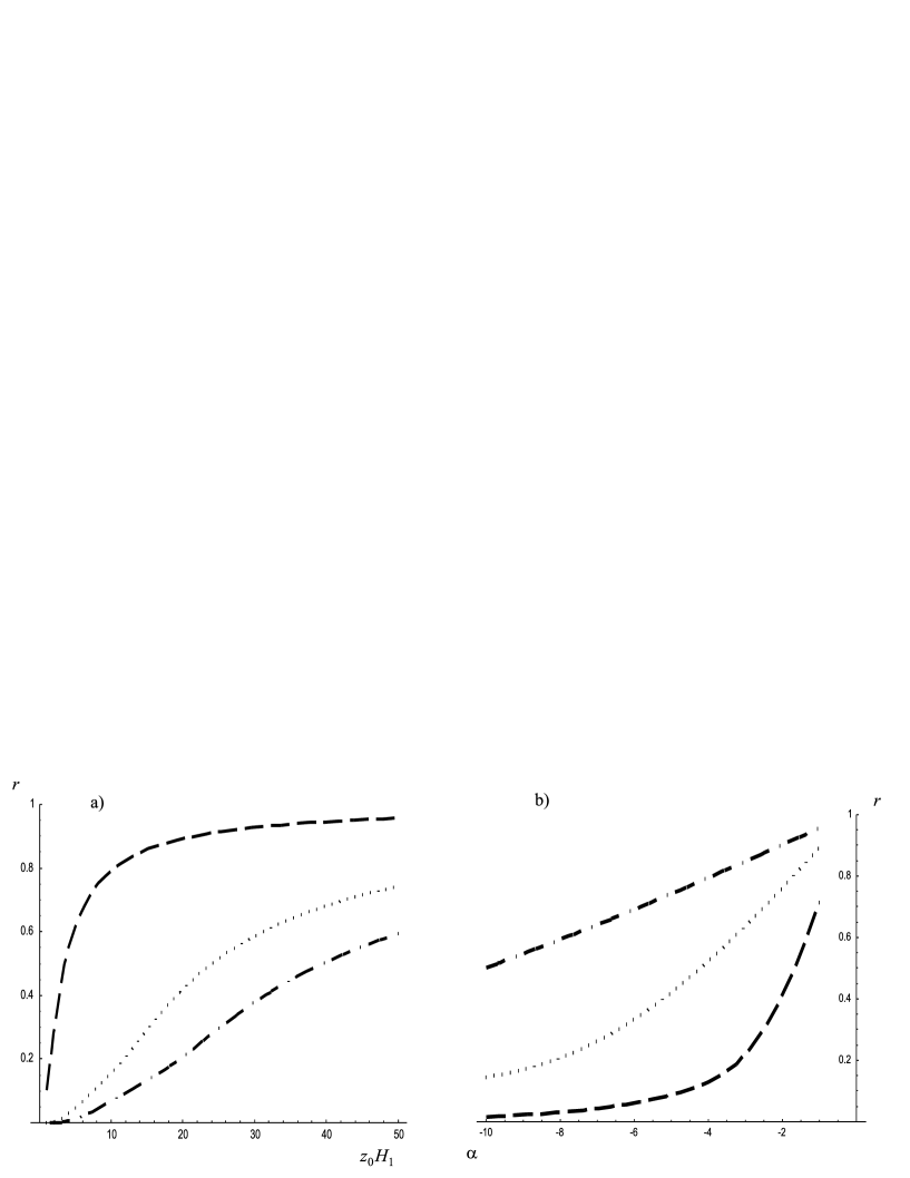
Figure 4: Plot a) shows the behaviour of $r$ with respect to $z_{0}H_{1}$ for the three values of $\alpha$ used elsewhere: $\alpha=-1$ (dashed line), $\alpha=-5$ (dotted line) and $\alpha=-8$ (dot-dashed line). Plot b) is complementary to the first one, and shows the behaviour of $r$ with respect to $\alpha$ for the three different values of $z_{0}H_{1}=7$ (dashed line), $z_{0}H_{1}=20$ (dotted line) and $z_{0}H_{1}=50$ (dot-dashed line).

As we can see, the KK contribution is very low at small values of $z_{0}H_{1}$; however, it rapidly increases, to become completely dominant in the high energy regime, differently from what happens in other models present in the literature [5, 6, 7, 11]. Of course, this effect could in principle be relevant in observational tests concerning the amplification of tensor perturbation during inflation. Actually, since the spectrum obtained in our simple evolution model increases with the frequency, it is not difficult to tune the free parameters so as to satisfy COBE and pulsar constraints. Moreover, the relevance of the massive modes contribution can be lowered by the presence of the dilaton. In fact, at relatively high energies, the effect of the bulk gravitons can be very strong if the dilaton is absent or weakly coupled, but it becomes negligible as the coupling increases. This indicates that, even at high energies, the enhancement of the amplitude of the KK spectrum can be “cured” by a suitable choice of coupling parameter, leading to a spectrum that is quite similar to the 4-dimensional one.

The decisive test for models with strong production of KK modes will be the future detection of stochastic gravitational waves at gravitational antennae. For this purpose, more accurate and realistic models are needed, in which the presence of matter on the brane is taken into account, and a smooth transition from the inflationary to the standard cosmological evolution is considered. This will be the subject of forthcoming papers to investigate which features of the simple model under discussion can be generalized to these more realistic models.

References

• [1] L. Randall and R. Sundrum, “An alternative to compactification”, Phys. Rev. Lett.  83, 4690 (1999) [arXiv:hep-th/9906064].
• [2] R. Maartens, “Brane-world gravity”, Living Rev. Rel.  7, 7 (2004) [arXiv:gr-qc/0312059].
• [3] N. Deruelle, T. Dolezel and J. Katz, “Perturbations of brane worlds” Phys. Rev. D 63, 083513 (2001) [arXiv:hep-th/0010215].
• [4] K. Koyama and J. Soda, “Evolution of cosmological perturbations in the brane world”, Phys. Rev. D 62, 123502 (2000) [arXiv:hep-th/0005239].
• [5] D. Langlois, R. Maartens and D. Wands, “Gravitational waves from inflation on the brane”, Phys. Lett. B 489, 259 (2000) [arXiv:hep-th/0006007].
• [6] D. S. Gorbunov, V. A. Rubakov and S. M. Sibiryakov, “Gravity waves from inflating brane or mirrors moving in adS(5)”, JHEP 0110, 015 (2001) [arXiv:hep-th/0108017].
• [7] T. Kobayashi, H. Kudoh and T. Tanaka, “Primordial gravitational waves in inflationary brane-world”, Phys. Rev. D 68, 044025 (2003) [arXiv:gr-qc/0305006].
• [8] R. Easther, D. Langlois, R. Maartens and D. Wands, “Evolution of gravitational waves in Randall-Sundrum cosmology”, JCAP 0310, 014 (2003) [arXiv:hep-th/0308078].
• [9] M. Cavaglia, G. De Risi and M. Gasperini, “Relic gravitons on Kasner-like branes”, Phys. Lett. B 610, 9 (2005) [arXiv:hep-th/0501251].
• [10] C. Cartier, R. Durrer and M. Ruser, “On graviton production in brane-world cosmology”, Phys. Rev. D 72, 104018 (2005) [arXiv:hep-th/0510155].
• [11] T. Kobayashi and T. Tanaka, “The spectrum of gravitational waves in Randall-Sundrum brane-world cosmology”, Phys. Rev. D 73, 044005 (2006) [arXiv:hep-th/0511186].
• [12] R. Maartens, D. Wands, B. A. Bassett and I. Heard, “Chaotic inflation on the brane”, Phys. Rev. D 62, 041301 (2000) [arXiv:hep-ph/9912464].
• [13] K. i. Maeda and D. Wands, “Dilaton-gravity on the brane”, Phys. Rev. D 62, 124009 (2000) [arXiv:hep-th/0008188].
• [14] V. Bozza, M. Gasperini and G. Veneziano, “Localization of scalar fluctuations in a dilatonic brane world scenario”, Nucl. Phys. B 619, 191 (2001) [arXiv:hep-th/0106019].
• [15] K. Koyama and K. Takahashi, “Primordial fluctuations in bulk inflaton model”, Phys. Rev. D 67, 103503 (2003) [arXiv:hep-th/0301165].
• [16] K. Koyama and K. Takahashi, “Exactly solvable model for cosmological perturbations in dilatonic brane worlds”, Phys. Rev. D 68, 103512 (2003) [arXiv:hep-th/0307073].
• [17] T. Kobayashi and T. Tanaka, “Bulk inflaton shadows of vacuum gravity”, Phys. Rev. D 69, 064037 (2004) [arXiv:hep-th/0311197].
• [18] W. Israel, “Singular hypersurfaces and thin shells in General Relativity”, Nuovo Cim. B 44S10:1, (1966) [Erratum-ibid. B 48, 463 (1967 NUCIA,B44,1.1966)].
• [19] T. Shiromizu, K. i. Maeda and M. Sasaki, “The Einstein equations on the 3-brane world”, Phys. Rev. D 62, 024012 (2000) [arXiv:gr-qc/9910076].
• [20] A. N. Aliev and A. E. Gumrukcuoglu, “Gravitational field equations on and off a 3-brane world”, Class. Quant. Grav.  21, 5081 (2004) [arXiv:hep-th/0407095].
• [21] M. Gasperini and G. Veneziano, “Pre-big bang in string cosmology”, Astropart. Phys.  1, 317 (1993) [arXiv:hep-th/9211021].
• [22] M. Gasperini and G. Veneziano, “The pre-big bang scenario in string cosmology”, Phys. Rep.  373, 1 (2003) [arXiv:hep-th/0207130].
• [23] M. Cvetic, H. Lu and C. N. Pope, “Domain walls with localised gravity and domain-wall/QFT correspondence”, Phys. Rev. D 63, 086004 (2001) [arXiv:hep-th/0007209].
• [24] M. Maggiore, “Gravitational wave experiments and early Universe cosmology”, Phys. Rep.  331, 283 (2000) [arXiv:gr-qc/9909001].
• [25] J. Audretsch, “Cosmological particle creation ss above-barrier reflection: Approximation method and applications”, J. Phys. A 12, 1189 (1979).
• [26] A. E. Lawrence and E. J. Martinec, “String field theory in curved spacetime and the resolution of spacelike singularities”, Class. Quant. Grav.  13, 63 (1996) [arXiv:hep-th/9509149].
• [27] N. D. Birrell and P. C. W. Davies, “Quantum fields in curved space”, (Cambridge Univ. Press, Cambridge 1982).