A numerical investigation of the stability of steady states and critical phenomena for the spherically symmetric Einstein-Vlasov system

Abstract

The stability features of steady states of the spherically symmetric Einstein-Vlasov system are investigated numerically. We find support for the conjecture by Zeldovich and Novikov that the binding energy maximum along a steady state sequence signals the onset of instability, a conjecture which we extend to and confirm for non-isotropic states. The sign of the binding energy of a solution turns out to be relevant for its time evolution in general. We relate the stability properties to the question of universality in critical collapse and find that for Vlasov matter universality does not seem to hold.

1 Introduction

For any given dynamical system the existence and stability of steady states is essential both from a mathematics and from a physics point of view. In this paper we investigate these questions by numerical means for the spherically symmetric, asymptotically flat Einstein-Vlasov system. This system describes a self gravitating collisionless gas in the framework of general relativity. Here the matter is thought of as a large ensemble of particles, which is described by a density function on phase space, and the individual particles move along geodesics. The precise formulation of this system will be given in the next section; for further information on the Einstein-Vlasov system we refer to [1]. In astrophysics the system is used to model compact star clusters and galaxies. In this context the stability question was first studied by Zeldovich e. a. in the sixties [38, 37]. These authors characterize a steady state by its central redshift and binding energy and conjecture that the binding energy maximum along a steady state sequence signals the onset of instability. For isotropic steady states Ipser [17] and Shapiro and Teukolsky [33] found numerical support for this conjecture. In our investigation we find that this conjecture holds for non-isotropic steady states as well, where the density on phase space depends on the particle energy and angular momentum. Moreover, we use three different kinds of perturbations (for details see Section 3) while in the previous studies mentioned above only one type of perturbation was implemented. We also find that the sign of the binding energy is crucial for the evolution of the perturbed solutions. A positive value implies that the solution is bound in the sense that not all matter can disperse to infinity, and in this case the perturbation of a stable state seems to lead to periodic oscillations. In the case of a negative value of the binding energy we observe that the solution disperses to infinity.

Our initial motivation for studying the stability of steady states was its role in critical collapse. This topic started with the work of Choptuik [7] where he studied the Einstein-scalar-field system. He took a fixed initial profile for the scalar field and scaled it by an arbitrary constant factor. This gives rise to a family of initial data depending on a real parameter $A$. It turned out that there exists a critical parameter $A_{\ast}$ such that for $A<A_{\ast}$ the corresponding solutions disperses as predicted by the theoretical results of Christodoulou [9] for small data, while for $A>A_{\ast}$ the corresponding solutions collapse and produce a black hole in accordance with [10]. The surprising result was that the limit of the mass $M(A)$ of the black hole tends to zero for $A\to A_{\ast}$ so that in such a one-parameter family there are black holes with arbitrarily small mass. Choptuik found that this fact is related to the existence of self-similar solutions of the Einstein-scalar-field system, in particular, the critical solution is self-similar and universal, i.e., independent of the initial profile which determines the one-parameter family. Later on Choptuik, Chmaj, and Bizoń performed a similar investigation for the Einstein-Yang-Mills system [8]. Here both cases $\lim_{A\to A_{\ast}}M(A)=0$ and $\lim_{A\to A_{\ast},A>A_{\ast}}M(A)>0$ were found and called type II and type I respectively. In the latter case there is a mass gap in the $M(A)$-curve. The possibility of type I behavior in this system was related to the existence of the Bartnik-McKinnon solutions [5, 34], which are static. Again, the conjecture is that the critical solution is universal.

As opposed to the field theoretic matter models mentioned above the Vlasov model is phenomenological, and in contrast to fluid models several global results have been obtained for Vlasov matter. For the spherically symmetric, asymptotically flat case it was shown in [23] that sufficiently small initial data launch global, geodesically complete solutions which disperse for large times. It is also known that there do exist initial data, necessarily large, which develop singularities [29]. The proof relies on the Penrose singularity theorem. There are no general results on the behavior of large data solutions yet, except for the following: If data on a hypersurface of constant Schwarzschild time give rise to a solution which develops a singularity after a finite amount of Schwarzschild time, then the first singularity occurs at the center of symmetry [26]. An analogous result where Schwarzschild time is replaced by maximal slicing has also been proved [29]. In [2] further results on the global behavior of solutions for large data can be found. The transition between dispersion and gravitational collapse was numerically investigated by Rein, Rendall, and Schaeffer [27], and it was found that there is a mass gap in the $M(A)$ curve. This result was later confirmed by Olabarrieta and Choptuik [19]. In addition, the latter authors reported evidence that the mass gap is due to the presence of static solutions, and they found support that the critical solution is universal.

In the present investigation we address the role of steady states in critical phenomena for the Einstein-Vlasov system and the question of universality by explicitly exploiting the fact that for this system the existence of an abundance of steady states is well-established [25], and that these steady states can easily be computed numerically. Computing a steady state $f_{s}$ we consider the family $Af_{s}$ of initial data. Within every family of steady states given by a specific dependence on particle energy and angular momentum we find unstable ones which act as critical solutions: If they are perturbed with $A>1$ they collapse to a black hole, if they are perturbed with $A<1$ they either disperse or oscillate in a neighborhood of the steady state, depending on the sign of the binding energy. Due to the abundance of possible such dependences on particle energy and angular momentum there cannot be a universal critical solution in spherically symmetric collapse for the Einstein-Vlasov system.

The paper proceeds as follows: In the next section we formulate the Einstein-Vlasov system, first in general coordinates and then in coordinates adapted to spherical symmetry. In [27] Schwarzschild coordinates were used. Here we use maximal areal coordinates, as was done in [19]. This has the advantage that regions of spacetime containing trapped surfaces can be covered. In Section 3 we discuss the numerical scheme which we use; it is a particle-in-cell scheme of the type used for kinetic models in plasma physics. It should be noted that for the analogous scheme used in [27] a rigorous convergence proof has been established in [28], and we conjecture that this can be done for the present scheme as well. In Section 4 we investigate the stability properties of certain steady states and compare our findings with the earlier work mentioned above. Section 5 is devoted to critical phenomena and non-universality, and in a final section we discuss the reliability of our code.

Our main motivation for this numerical analysis is that it may lead to conjectures on the behavior of solutions of the Einstein-Vlasov system which may eventually be proven rigorously.

2 The Einstein-Vlasov system

We first write down the Einstein-Vlasov system in general coordinates on the tangent bundle $TM$ of the spacetime manifold $M$. Following standard practice we normalize the physical constants to one. The system then reads as follows:

$$p^{a}\partial_{x^{a}}f-\Gamma^{a}_{bc}p^{b}p^{c}\partial_{p^{a}}f=0,$$

$$G^{ab}=8\pi T^{ab},$$

$$T^{ab}=\int p^{a}p^{b}f\,|g|^{1/2}\,\frac{d^{4}p}{m}.$$

Here $f$ is the number density of the particles on phase space, $\Gamma^{a}_{bc}$ and $G^{ab}$ denote the Christoffel symbols and the Einstein tensor obtained from the spacetime metric $g_{ab}$, $|g|$ denotes its determinant, $T^{ab}$ is the energy-momentum tensor generated by $f$, $x^{a}$ are coordinates on $M$, $(x^{a},p^{b})$ the corresponding coordinates on the tangent bundle $TM$, Latin indices run from 0 to 3, and

$$m=|g_{ab}p^{a}p^{b}|^{1/2}$$

is the rest mass of a particle at the corresponding point in phase space. We assume that all particles have rest mass 1 and move forward in time so that the distribution function $f$ lives on the mass shell

$$PM=\Bigl{\{}g_{ab}p^{a}p^{b}=-1,\ p^{0}>0\Bigr{\}}.$$

We consider this system in the spherically symmetric, asymptotically flat case and write the metric in the following form:

$$ds^{2}=-(\alpha^{2}+a^{2}\beta^{2})dt^{2}+2a^{2}\beta dtdr+a^{2}dr^{2}+r^{2}\left(d\theta^{2}+\sin^{2}\theta\,d\phi^{2}\right).$$

Here the metric coefficients $\alpha,\beta$, and $a$ depend on $t\in\mathbb{R}$ and $r\geq 0$, $\alpha$ and $a$ are positive, and the polar angles $\theta\in[0,\pi]$ and $\phi\in[0,2\pi]$ parameterize the unit sphere. The radial coordinate $r$ is thus the area radius. Let $K^{a}_{b}$ be the second fundamental form and define

$$\kappa:=K^{\theta}_{\theta}=\frac{\beta}{r\alpha}.$$

By imposing the maximal gauge condition, which means that each hypersurface of constant $t$ has vanishing mean curvature, we obtain the following field equations:

$$\displaystyle a_{r}=\frac{3}{2}a^{3}r\kappa^{2}+4\pi ra^{3}\rho+\frac{a}{2r}(1-a^{2}),$$ (1)

$$\displaystyle\kappa_{r}=-\frac{3}{r}\kappa-4\pi a\jmath,$$ (2)

$$\displaystyle a_{t}=2\alpha a\kappa+(a\beta)_{r},$$ (3)

$$\displaystyle\alpha_{rr}=\alpha_{r}\left(\frac{a_{r}}{a}-\frac{2}{r}\right)+\frac{2\alpha}{r^{2}}\left(2r\frac{a_{r}}{a}+a^{2}-1\right)+4\pi a^{2}\alpha(S-3\rho).$$ (4)

The Vlasov equation takes the form

$$\partial_{t}f+\left(\frac{\alpha w}{a\epsilon}-\beta\right)\partial_{r}f+\left(-\frac{\alpha_{r}\epsilon}{a}-2\alpha\kappa w+\frac{\alpha L}{ar^{3}\epsilon}\right)\partial_{w}f=0,$$ (5)

where

$$\epsilon=\epsilon(r,w,L)=\sqrt{1+w^{2}+L/r^{2}}.$$ (6)

The variables $w$ and $L$ can be thought of as the momentum in the radial direction and the square of the angular momentum respectively, see [20] for more details. The matter quantities are defined by

$$\rho(t,r) = \frac{\pi}{r^{2}}\int_{-\infty}^{\infty}\int_{0}^{\infty}\epsilon f(t,r,w,L)\,dL\,dw,$$ (7)

$$\jmath(t,r) = \frac{\pi}{r^{2}}\int_{-\infty}^{\infty}\int_{0}^{\infty}wf(t,r,w,L)\,dL\,dw,$$ (8)

$$S(t,r) = \frac{\pi}{r^{2}}\int_{-\infty}^{\infty}\int_{0}^{\infty}\frac{w^{2}+L/r^{2}}{\epsilon}\,f(t,r,w,L)\,dL\,dw.$$ (9)

We impose the following boundary conditions which ensure asymptotic flatness and a regular center:

$$a(t,0)=a(t,\infty)=\alpha(t,\infty)=1.$$ (10)

The equations (1)–(9) together with the boundary conditions (10) constitute the Einstein-Vlasov system for a spherically symmetric, asymptotically flat spacetime in maximal areal coordinates.

Let us consider some simple properties of this system, in particular such as will be relevant for its numerical simulation; a more careful mathematical analysis of the system will be performed elsewhere [3]. First we note that the phase space density $f$ is constant along solutions of the characteristic system

$$\dot{r} = \frac{\alpha(\tau,r)w}{a(\tau,r)\epsilon}-\beta(\tau,r),$$ (11)

$$\dot{w} = -\frac{\alpha_{r}(\tau,r)\epsilon}{a(\tau,r)}-2\alpha(\tau,r)\kappa(\tau,r)w+\frac{\alpha(\tau,r)L}{a(\tau,r)r^{3}\epsilon},$$ (12)

$$\dot{L} = 0$$ (13)

of the Vlasov equation. If $\tau\mapsto(R,W,L)(\tau,t,r,w,L)=:Z(\tau,t,z)$ denotes the solution of the characteristic system with $(R,W,L)(t,t,r,w,L)=(r,w,L)$ then

$$f(t,r,w,L)=\vbox{\hbox{\hskip 2.38885pt\tiny$\circ$}\hbox{$f$}}\!((R,W,L)(0,t,r,w,L)),$$

with $\vbox{\hbox{\hskip 2.38885pt\tiny$\circ$}\hbox{$f$}}\!=f(0,\cdot)$ the initial datum for $f$. Due to our choice of coordinates $w,L$ in momentum space the characteristic flow is not measure preserving. Indeed, if by $D$ we denote differentiation along a characteristic of the Vlasov equation, then

$$D(f\,dL\,dw\,dr)=-\left(\frac{\alpha w}{a^{2}\epsilon}a_{r}+\beta_{r}+\frac{2\beta}{r}\right)\,f\,dL\,dw\,dr;$$ (14)

the factor on the right hand side is the $(r,w,L)$-divergence of the right hand side of the characteristic system. Notice that by Eqn. (3) this factor equals $-D\ln a$. If $A\subset\mathbb{R}_{+}\times\mathbb{R}\times\mathbb{R}_{+}$ is measurable and $A(t):=Z(t,0,A)=\{(R,W,L)(t,0,r,w,L)\mid(r,w,L)\in A\}$ then

$$\int_{A(t)}f(t,z)\,dz=\int_{A}\vbox{\hbox{\hskip 2.38885pt\tiny$\circ$}\hbox{$f$}}\!(z)\frac{a(0,r)}{a(t,R(t,0,z))}dz,$$

while

$$\int_{A(t)}a(t,r)\,f(t,z)\,dz=\int_{A}a(0,r)\,\vbox{\hbox{\hskip 2.38885pt\tiny$\circ$}\hbox{$f$}}\!(z)\,dz.$$

In particular, the total number of particles, which, since all particles have rest mass one, equals the rest mass of the system, is conserved:

$$4\pi^{2}\int_{0}^{\infty}\int_{-\infty}^{\infty}\int_{0}^{\infty}a(t,r)f(t,r,w,L)\,dL\,dw\,dr=M_{0}.$$

Next we notice that Eqn. (2) can be rewritten as

$$\left(r^{3}\kappa\right)_{r}=-4\pi r^{3}a\jmath.$$ (15)

Using Eqn. (1) the second order equation (4) can be rewritten as

$$\left(\frac{r^{2}}{a}\alpha_{r}\right)_{r}=4\pi r^{2}a\alpha(\rho+S)+6r^{2}a\alpha\kappa^{2}.$$ (16)

The Hawking mass $m$ is given by

$$m=\frac{r}{2}\left(1+\frac{\beta^{2}}{\alpha^{2}}-\frac{1}{a^{2}}\right).$$ (17)

We also introduce the quantity

$$\mu:=\frac{r}{2}\left(1-\frac{1}{a^{2}}\right),$$

and note that by Eqn. (1), $\mu$ can be written in the form

$$\mu(t,r)=\int_{0}^{r}\left(4\pi\rho(t,s)+\frac{3}{2}\kappa^{2}(t,s)\right)s^{2}ds.$$

Assuming that the matter is compactly supported initially and hence also for later times Eqn. (15) implies that $\kappa(t,r)\sim r^{-3}$ for $r$ large. Hence the limits as $r$ tends to $\infty$ of $m$ and $\mu$ are equal so that the ADM mass $M$ can be written as

$$M=\int_{0}^{\infty}\left(4\pi\rho(t,r)+\frac{3}{2}\kappa^{2}(t,r)\right)r^{2}dr.$$

The ADM mass is conserved.

It is of interest to find out when trapped surfaces form, which means that $2m/r>1,$ and in view of (17) this condition can be written as

$$a^{2}>\frac{\alpha^{2}}{\beta^{2}}.$$

Note also that $2m/r<1/2$ implies that $2\mu/r<1/2$. From [18] we obtain the following inequalities

$$\left|\frac{1}{a}-\frac{\beta}{\alpha}\right|\leq 1,\;\;\left|\frac{1}{a}+\frac{\beta}{\alpha}\right|\leq 1.$$ (18)

Finally we notice that the second order equation for $\alpha$ in the form (16) can be integrated:

$$\alpha_{r}(t,r)=\frac{a(t,r)}{r^{2}}\int_{0}^{r}\left(4\pi\alpha a(\rho+S)+6a\alpha\kappa^{2}\right)s^{2}ds.$$ (19)

Thus $\alpha$ is monotonically increasing outwards, and from (10) and (18) it follows that

$$0<\alpha\leq 1,\ |\beta|\leq\alpha\leq 1.$$

3 The numerical method

Let us consider an initial condition $\vbox{\hbox{\hskip 2.38885pt\tiny$\circ$}\hbox{$f$}}\!=\vbox{\hbox{\hskip 2.38885pt\tiny$\circ$}\hbox{$f$}}\!(r,w,L)$, define additional variables $u\geq 0$ and $\phi\in[0,\pi]$ by the relations

$$u^{2}=w^{2}+\frac{L}{r^{2}},\ w=u\,\cos\phi,\ L=r^{2}u^{2}\sin^{2}\phi$$

and assume that  $\circ$ $f$ vanishes outside the set $(r,u,\phi)\in[R_{0},R_{1}]\times[U_{0},U_{1}]\times[\Phi_{0},\Phi_{1}]$. We will approximate the solution using a particle method. For a thorough treatment of particle methods in the context of plasma physics we refer to [6]. To initialize the particles we take integers $N_{r},N_{u},N_{\phi}$ and define

$$\Delta r=\frac{R_{1}-R_{0}}{N_{r}},\ \Delta u=\frac{U_{1}-U_{0}}{N_{u}},\ \Delta\phi=\frac{\Phi_{1}-\Phi_{0}}{N_{\phi}},$$

$$r_{i}=R_{0}+\left(i-\frac{1}{2}\right)\Delta r,\ u_{j}=U_{0}+\left(j-\frac{1}{2}\right)\Delta u,\ \phi_{k}=\Phi_{0}+\left(k-\frac{1}{2}\right)\Delta\phi,$$

$$f^{0}_{ijk}=\vbox{\hbox{\hskip 2.38885pt\tiny$\circ$}\hbox{$f$}}\!\left(r_{i},u_{j},\phi_{k}\right)\;4\pi r^{2}_{i}\Delta r\;2\pi u^{2}_{j}\Delta u\,\sin\phi_{k}\Delta\phi,$$

$$r^{0}_{ijk}=r_{i},\ w^{0}_{ijk}=u_{j}\,\cos\phi_{k},\ L_{ijk}=\left(r_{i}u_{j}\,\sin\phi_{k}\right)^{2}.$$

At this point it should be noted that $f^{0}_{ijk}$ contains the phase space volume element, a fact which is convenient when computing the induced components of the energy momentum tensor, but which has to be observed when this quantity is time-stepped. At each point in phase space with coordinates $r^{0}_{ijk},w^{0}_{ijk},L_{ijk}$ we imagine a particle with weight $f^{0}_{ijk}$ which is smeared out in the radial direction, i.e., with respect to $r$ it is represented by a hat function of width $2\Delta r$. Once the particles are initialized the grid covering the support of the initial datum plays no further role. From these numerical particles, approximations are made of the quantities $\rho,\ \jmath,\ S$ defined in (7), (8), (9) at the spatial grid points

$$r_{j}:=j\Delta r,\ j=0,\ldots,N+1;$$

note that this is now a new grid, which we extend from $r=0$ to the radius of the spatial support of the matter quantities. The field equations (1) and (15), which do not contain the metric coefficient $\alpha$, can now be integrated on the support of the matter from the origin outward, using the boundary conditions (10) and $(r^{3}\kappa)_{|r=0}=0$; notice that $\kappa$ is then also known outside the support of the matter.

To obtain an approximation of the metric coefficient $\alpha$ at the grid points $r_{j}$ we discretize Eqn. (16) in the following way: We write

$$r_{j+\frac{1}{2}}:=\left(j+\frac{1}{2}\right)\Delta r,$$

and from what is already computed we obtain approximations for $a$, $\kappa$, $\rho$, $S$ both at the grid points $r_{j}$ and by interpolation at the intermediate points $r_{j+\frac{1}{2}}$, which we denote by

$$a_{j},\ a_{j+\frac{1}{2}},\ \ldots$$

Using the approximations

$$\left(\frac{r^{2}}{a}\alpha_{r}\right)_{r}(r_{j})\approx\frac{1}{\Delta r}\left[\frac{r_{j+\frac{1}{2}}^{2}\alpha_{r}(r_{j+\frac{1}{2}})}{a_{j+\frac{1}{2}}}-\frac{r_{j-\frac{1}{2}}^{2}\alpha_{r}(r_{j-\frac{1}{2}})}{a_{j-\frac{1}{2}}}\right]$$

and

$$\alpha_{r}(r_{j+\frac{1}{2}})\approx\frac{\alpha_{j+1}-\alpha_{j}}{\Delta r},\ \alpha_{r}(r_{j-\frac{1}{2}})\approx\frac{\alpha_{j}-\alpha_{j-1}}{\Delta r}$$

we obtain the following linear system for the approximations $\alpha_{j}$ for $\alpha(r_{j})$ on the grid points: For $j=0,\ldots,N-1$,

$$\frac{r_{j+\frac{1}{2}}^{2}}{a_{j+\frac{1}{2}}}\alpha_{j+1} + \frac{r_{j-\frac{1}{2}}^{2}}{a_{j-\frac{1}{2}}}\alpha_{j-1}-$$

$$- \left[\frac{r_{j+\frac{1}{2}}^{2}}{a_{j+\frac{1}{2}}}+\frac{r_{j-\frac{1}{2}}^{2}}{a_{j-\frac{1}{2}}}+\left[6\kappa_{j}^{2}+4\pi(\rho_{j}+S_{j})\right]r_{j}^{2}(\Delta r)^{2}a_{j}\right]\alpha_{j}=0,$$

and

$$\alpha_{1}-\alpha_{0}=0,\ \alpha_{N+1}=\sqrt{1-\frac{2M^{\ast}}{r_{N+1}}}.$$

The last two equations arise from the boundary condition

$$\left(\frac{r^{2}}{a}\alpha_{r}\right)_{r}(t,0)=0$$

and the approximation

$$\alpha(t,r)\approx\sqrt{1-\frac{2\mu(t,r)}{r}}$$

for $r$ large, in particular, $r$ well outside the support of the matter. The latter approximation is motivated by the known representation of the asymptotically flat Schwarzschild solution in maximal areal coordinates. The approximation $M^{\ast}$ for $\mu(t,r)$ at large values of $r$ can be computed from the already approximated quantities $\rho$ and $\kappa$.

The linear system for $\alpha_{j}$ is tridiagonal, obviously diagonally dominated, and it can easily be solved. Thus we now have approximations for all the field quantities on the spatial grid points $r_{j}$. In passing we note that in [19] the field equation (4) was discretized directly resulting again in a tridiagonal system for $\alpha_{j}$, but our approach of discretizing the rewritten version (16) instead seems to perform better numerically.

To perform the time step we propagate the numerical particles according to the characteristic system of the Vlasov equation (11), (12), (13). To do so we interpolate the field quantities to particle locations and use a simple Euler time stepping method to define the new phase space coordinates $r^{1}_{ijk},w^{1}_{ijk},L^{1}_{ijk}$ of the numerical particle with label $ijk$. We still need to propagate the phase space volume element along the characteristics. Discretizing (14) in time we obtain the relation

$$\frac{1}{\Delta t}\left(f^{1}_{ijk}-f^{0}_{ijk}\right)=-\left(\frac{\alpha w}{a^{2}\epsilon}a_{r}+\beta_{r}+\frac{2\beta}{r}\right)\,f^{0}_{ijk}$$

which we use to compute $f^{1}_{ijk}$, and one time step is complete.

4 Stability issues for steady states

For static solutions, $\beta=\kappa=\jmath=0$ so that

$$m(r)=\mu(r)=4\pi\int_{0}^{r}\rho(s)\,s^{2}ds,$$

and the field equation (1) decouples and is solved by

$$a(r)=\left(1-\frac{2m(r)}{r}\right)^{-1/2}.$$ (20)

The metric coefficient $\alpha$ is determined by the equation

$$\frac{\alpha^{\prime}}{\alpha}=a^{2}\left(\frac{m}{r^{2}}+4\pi rp\right)$$ (21)

where $\alpha^{\prime}=\alpha_{r}=d\alpha/dr$ and

$$p(r):=\frac{\pi}{r^{2}}\int_{-\infty}^{\infty}\int_{0}^{\infty}\frac{w^{2}}{\epsilon}f(r,w,L)\,dL\,dw$$

is the radial pressure. Eqn. (21) is the $rr$-component of the Einstein equations, and a lengthy computation using the Tolman-Oppenheimer-Volkov equation

$$p^{\prime}=-\frac{\alpha^{\prime}}{\alpha}(p+\rho)-\frac{2}{r}(p-p_{T})$$

shows that the second order field equation (4) follows;

$$p_{T}(r):=\frac{\pi}{2r^{2}}\int_{-\infty}^{\infty}\int_{0}^{\infty}\frac{L}{\epsilon r^{2}}f(r,w,L)\,dL\,dw$$

is the tangential pressure. It is easy to check that in addition to $L$ also the particle energy

$$E:=\alpha(r)\sqrt{1+w^{2}+\frac{L}{r^{2}}}=\alpha(r)\epsilon$$

is constant along characteristics in the static case. Hence the ansatz

$$f(r,w,L)=\Phi(E,L),$$ (22)

satisfies the static Vlasov equation. By substituting it into the definitions for $\rho$ and $p$ these quantities become functionals of $\alpha$, and the static Einstein-Vlasov system is reduced to the equation (21) with (20) substituted in. Given some ansatz function $\Phi$ and prescribing some value for $\alpha(0)$, the static system can therefore easily be solved numerically, by integrating (21) from $r=0$ outward, in particular if $\Phi$ is such that the resulting dependence of $\rho$ and $p$ on $\alpha$ can be computed explicitly. This is the case for the power law

$$f(r,w,L)=\Phi(E,L)=(E_{0}-E)^{k}_{+}(L-L_{0})_{+}^{l}.$$ (23)

Here $l>-1/2,\,k>-1,\,L_{0}\geq 0$, $E_{0}>0$ is the cut-off energy, and $x_{+}:=\max\{x,0\}$. In the Newtonian case with $l=L_{0}=0$ this ansatz leads to steady states with a polytropic equation of state. Note that by taking $L_{0}>0$ there will be no matter in the region

$$r<\sqrt{\frac{L_{0}}{(E_{0}/\alpha(0))^{2}-1}},$$

since there necessarily $E>E_{0}$ and $f$ vanishes. We call such configurations static shells. The existence of static shells with finite mass and finite extension has been proved in [21]. It is numerically convenient to work with shells since potential difficulties in treating $r=0$ are avoided, and we will only consider shells here. This is also motivated by the fact that in the numerical experiments performed on critical phenomena in [27] the initial data for the matter had such a shell structure so that static shells are natural candidates for the critical solutions. It should be pointed out that there are static solutions which do not have the form (22), cf. [31].

In our simulations we have studied four cases:
          Case 1: $k=0,\,l=0$, Case 2: $k=0,\,l=1/2$, Case 3: $k=1,\,l=1/2$, Case 4: $k=0,\,l=3/2$.
Having chosen $k$ and $l$ we then numerically construct static solutions to the Einstein-Vlasov system as indicated above, by specifying values on $E_{0},\,L_{0}$ and $\alpha(0)$. The resulting metric coefficient will a-priori not satisfy the boundary condition $\alpha(\infty)=1$, but by shifting both $\alpha$ and $E_{0}$ appropriately a steady state which satisfies the boundary conditions is obtained. The distribution function $f_{s}$ of the steady state is then multiplied by an amplitude $A,$ so that a new, perturbed distribution function is obtained. This is then used as initial datum in our evolution code. Accordingly, if we choose $A=1$ then the initial datum is exactly the steady state, and a good test of our code is to check how much it deviates from being static in the evolution. We find that such initial data are tracked extremely well which is a very satisfying feature of our code. Of course, for unstable steady states the numerical errors introduced will make the solution drift off after some time which can be made longer by increasing the number of numerical particles and the number of time steps.

For $k$ and $l$ fixed we characterize each steady state by its central red shift $Z_{c}$ and its fractional binding energy $E_{b},$ which are defined by

$$Z_{c}=\frac{1}{\sqrt{\alpha(0)}}-1,\;\;E_{b}=\frac{e_{b}}{M_{0}},\mbox{ where }\;\;e_{b}=M_{0}-M.$$

The central redshift is the redshift of a photon emitted from the center and received at infinity, and the binding energy $e_{b}$ is the difference of the rest mass and the ADM mass and is a conserved quantity. In Figure 1 and Figure 2 below the relation between the fractional binding energy and the central redshift is given for Case 1 and Case 4 with $L_{0}=0.1$.

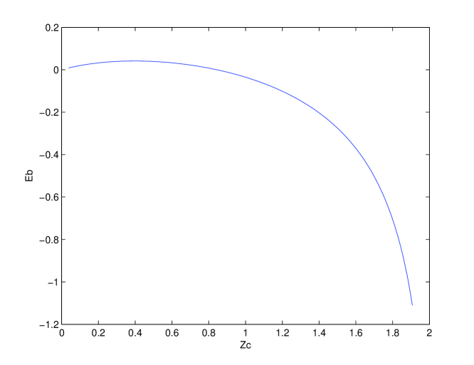
Figure 1: Case 1 with $L_{0}=0.1$

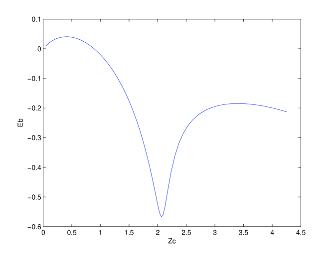
Figure 2: Case 4 with $L_{0}=0.1$

The relevance of these concepts for the stability properties of steady states was first discussed by Zeldovich and Podurets [38] who argued that it should be possible to diagnose the stability from binding energy considerations. Zeldovich and Novikov [37] then conjectured that the binding energy maximum along a steady state sequence signals the onset of instability. Ipser [17] and Shapiro and Teukolsky [33] find numerical support for this conjecture and they also find that steady states with a central redshift above about $0.5$ result in collapse and are thus unstable. In both of these studies only isotropic steady states were considered, i.e. $\Phi=\Phi(E),$ whereas our study includes the dependence on $L.$ Moreover, our algorithm is closely related to the one in [27] for which convergence has been proved in [28]. Of course, we also take advantage of the great progress of the computer capacity in that we can use a larger number of particles and considerably improve the resolution of the grid compared to what was possible in the earlier simulations. To get an indication of the accuracy of our simulation we compute at every time step the ADM mass $M$ and the rest mass $M_{0}$, both of which should be conserved, and as long as no trapped surface has formed the errors are remarkably small. We will get back to a discussion of the numerical errors in the final section.

Before describing the results of our simulations we mention that besides perturbations of a steady state $f_{s}$ of the form $Af_{s}$ we also considered perturbations of the form $f_{s}(r+r_{sh},w,L)$ and $f_{s}(r,w+w_{sh},L)$ where the state is shifted with respect to $r$ by $r_{sh}$ or with respect to $w$ by $w_{sh}$. It turns out that perturbations with $A>1$ or $r_{sh}<0$ or $w_{sh}<0$, which in principle push the state towards collapse, and on the other hand perturbations with $A<1$ or $r_{sh}>0$ or $w_{sh}>0$, which in principle push the state towards dispersion, lead to the same qualitative features of the perturbed solution. In the following discussion we restrict ourselves to perturbations of the form $Af_{s}$.

The general picture that arises from our simulations is summarized in Tables 1–4 which correspond to the four different cases we consider. The parameter $L_{0}$ is the same in all cases, i.e. $L_{0}=0.1.$

$Z_{c}$	$E_{b}$	$A<1$	$A>1$
$0.24$	$0.036$	stable	stable
$0.30$	$0.039$	stable	stable
$0.39$	$0.041$	stable	stable
$0.43$	$0.041$	stable	unstable
$0.47$	$0.040$	stable	unstable
$0.52$	$0.038$	stable	unstable
$0.65$	$0.027$	stable	unstable
$0.82$	$0.004$	stable	unstable
$0.95$	$-0.024$	unstable	unstable
$1.1$	$-0.070$	unstable	unstable

Table 1: Case 1: $k=0$ and $l=0.$

$Z_{c}$	$E_{b}$	$A<1$	$A>1$
$0.21$	$0.032$	stable	stable
$0.34$	$0.040$	stable	stable
$0.39$	$0.040$	stable	stable
$0.42$	$0.041$	stable	unstable
$0.46$	$0.040$	stable	unstable
$0.56$	$0.036$	stable	unstable
$0.65$	$0.029$	stable	unstable
$0.82$	$0.008$	stable	unstable
$0.95$	$-0.015$	unstable	unstable
$1.20$	$-0.078$	unstable	unstable

Table 2: Case 2: $k=0$ and $l=1/2.$

$Z_{c}$	$E_{b}$	$A<1$	$A>1$
$0.21$	$0.030$	stable	stable
$0.33$	$0.037$	stable	stable
$0.38$	$0.038$	stable	stable
$0.42$	$0.039$	stable	stable
$0.045$	$0.039$	stable	unstable
$0.052$	$0.037$	stable	unstable
$0.77$	$0.020$	stable	unstable
$0.90$	$0.004$	stable	unstable
$1.0$	$-0.01$	unstable	unstable
$1.13$	$-0.037$	unstable	unstable

Table 3: Case 3: $k=1$ and $l=1/2.$

$Z_{c}$	$E_{b}$	$A<1$	$A>1$
$0.21$	$0.032$	stable	stable
$0.34$	$0.039$	stable	stable
$0.41$	$0.040$	stable	stable
$0.44$	$0.040$	stable	stable
$0.52$	$0.038$	stable	unstable
$0.69$	$0.025$	stable	unstable
$0.80$	$0.014$	stable	unstable
$0.92$	$-0.004$	unstable	unstable
$1.1$	$-0.045$	unstable	unstable

Table 4: Case 4: $k=0$ and $l=3/2.$

If we first consider perturbations with $A>1$ we find that steady states with small values on $Z_{c}$ (less than approximately $0.40$ depending on which case we consider) are stable, i.e., the perturbed solutions stay in a neighborhood of the static solution as depicted in Figure 3.

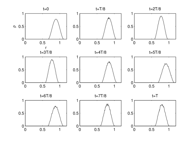
Figure 3: $Z_{c}=0.30,\ E_{b}=0.04,\ A=1.01,\ T=80.0$

A more careful investigation of these perturbed solutions seems to indicate that they oscillate in an (almost) periodic way, and we come back to this issue at the end of this section. For larger values of $Z_{c}$ the evolution leads to the formation of trapped surfaces and by the result in [11] to the collapse to black holes, as depicted in Figure 4.

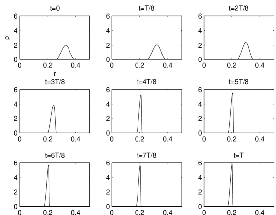
Figure 4: $Z_{c}=1.14,\ E_{b}=-0.08,\ A=1.01,\ T=10.0$

As a matter of fact we do check if null geodesics that start after a certain time from the center are caught so that they cannot escape to infinity, and our results always support that there is an event horizon.

Hence, for perturbations with $A>1$ the value of $Z_{c}$ alone seems to determine the stability features of the steady states. By plotting the curve, $E_{b}$ versus $Z_{c},$ for a shorter interval of $Z_{c}$ to get better resolution (Figures 5 and 6 below) we find that the conjecture by Novikov and Zeldovich, that the maximum of $E_{b}$ along a sequence of steady states signals the onset of instability, is true in a numerical sense also for states that depend on the angular momentum $L$.

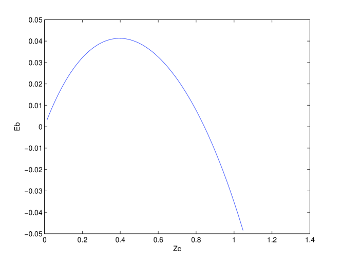
Figure 5: Case 1 with $L_{0}=0.1$

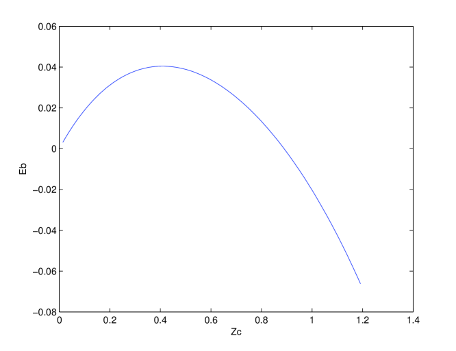
Figure 6: Case 4 with $L_{0}=0.1$

Having a second look at Figure 2 one might think that along that curve another change of stability behavior might occur at $Z_{c}\approx 2$, but we found no indication of this. The reason for the qualitative difference between Figure 1 and Figure 2 and its possible consequences will be investigated elsewhere [4].

The situation is quite different for perturbations with $A<1$. The crucial quantity in this case is the fractional binding energy $E_{b}$. Consider a steady state with $E_{b}>0$ and a perturbation with $A<1$ but close to $1$ so that the fractional binding energy remains positive. Then the perturbed solution drifts outwards and then turns back and reimplodes and comes close to its initial state, and then continues to expand and reimplode and thus oscillates. This is depicted in Figure 7, see also the end of this section.

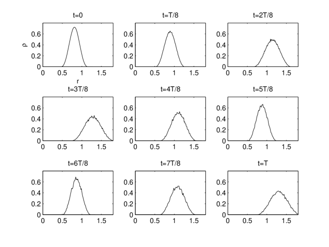
Figure 7: $Z_{c}=0.47,\ E_{b}=0.04,\ A=0.99,\ T=90.0$

In [33] it is stated that if $E_{b}>0$ the solution must ultimately reimplode. We are not aware of any precise mathematical formulation (or proof) of such a statement but our simulations support that it is true. For negative values of $E_{b}$ the solutions with $A<1$ disperse to infinity as depicted in Figure 8.

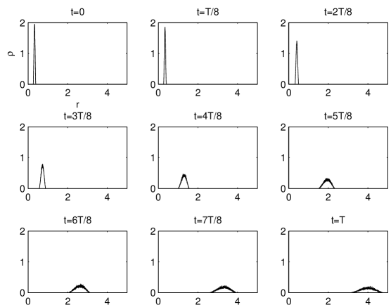
Figure 8: $Z_{c}=1.14,\ E_{b}=-0.08,\ A=0.99,\ T=14.0$

A simple argument which relates the binding energy to the question whether a solution disperses or not at least for the case where the spatial support is a shell is the following: Consider a solution which has an expanding vacuum region of radius $R(t)$ at the center with $R(t)\to\infty$ for $t\to\infty$. Such a solution disperses in a strong sense, and we claim that this implies that $M_{0}\leq M$, i.e. $E_{b}\leq 0$. To see this, observe that

$$M_{0} = 4\pi^{2}\int_{R(t)}^{\infty}\int_{-\infty}^{\infty}\int_{0}^{\infty}a(t,r)\,f(t,r,w,L)\,dL\,dw\,dr$$

$$= 4\pi^{2}\int_{R(t)}^{\infty}\left(1-\frac{2\mu(t,r)}{r}\right)^{-1/2}\int_{-\infty}^{\infty}\int_{0}^{\infty}f(t,r,w,L)\,dL\,dw\,dr$$

$$\leq \left(1-\frac{2M}{R(t)}\right)^{-1/2}4\pi^{2}\int_{R(t)}^{\infty}\int_{-\infty}^{\infty}\int_{0}^{\infty}\epsilon f(t,r,w,L)\,dL\,dw\,dr$$

$$= \left(1-\frac{2M}{R(t)}\right)^{-1/2}M,$$

so that with $t\to\infty$ necessarily $M_{0}\leq M$ as claimed.

For the Vlasov-Poisson system, which is the Newtonian limit of the Einstein-Vlasov system [24] a rigorous stability theory for steady states of the form analogous to (22) has been developed in recent years, based on variational techniques, cf. [13, 14, 15, 16, 22]. The result is that the stability properties of the steady state are essentially determined by the ansatz function $\Phi$ in (22), in particular, all the polytropic steady states resulting from an ansatz of the form (23) with $0<k<7/2,\ l=0,\ L_{0}=0$ are nonlinearly stable. The above discussion shows that an analogous result does not hold for the Einstein-Vlasov system, since there the stability depends in addition on the central redshift and the binding energy, even if $k$ and $l$ are fixed. We note at this point that the stability of shell like steady states has not yet been systematically investigated for the Vlasov-Poisson system. But we would argue that this does not affect the above statement, since on the one hand it is reasonable to expect that the stability results for shells in the Newtonian case will be analogous to the case $L_{0}=0$, an expectation supported by recent results in this direction [32], and on the other hand we do not expect our numerical stability results for the relativistic case to depend on the shell structure of the steady states. A clear indication that stability results based on variational techniques do not carry over to the relativistic case without making additional restrictions are the first results in this direction in [36].

Our investigation indicates that there are (at least) three qualitatively different types of behavior which can result from the perturbation of a steady state. Perturbing an unstable state with $Z_{c}>0.4$ using $A>1$ leads to gravitational collapse and a black hole. Perturbing an unstable state with $E_{b}<0$ using $A<1$ leads to dispersion. In the other, stable cases $Z_{c}<0.4$ and $A>1$ or $E_{b}>0$ and $A<1$ the perturbation leads to an oscillatory behavior. Whether the perturbed solution is indeed time-periodic is hard to decide numerically. One way to shed some light on this question is to plot $\alpha(t,0)$ or the inner and outer radius $r_{\mathrm{min}}(t)$ and $r_{\mathrm{max}}(t)$ of the matter support. The results are shown in Figures 9 and 10 for a steady state with $k=0,l=1/2$ (Case 2) and $L_{0}=0.1,\ Z_{c}=0.21,\ E_{b}=0.03$, perturbed with $A=1.02$.

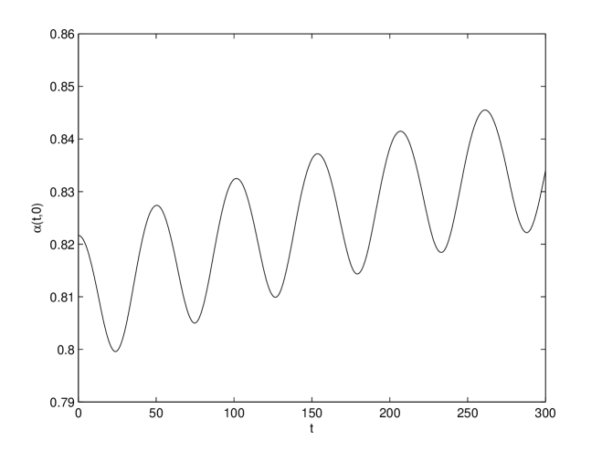
Figure 9: $Z_{c}=0.21,\ E_{b}=0.03,\ A=1.02,\ T=300.0$

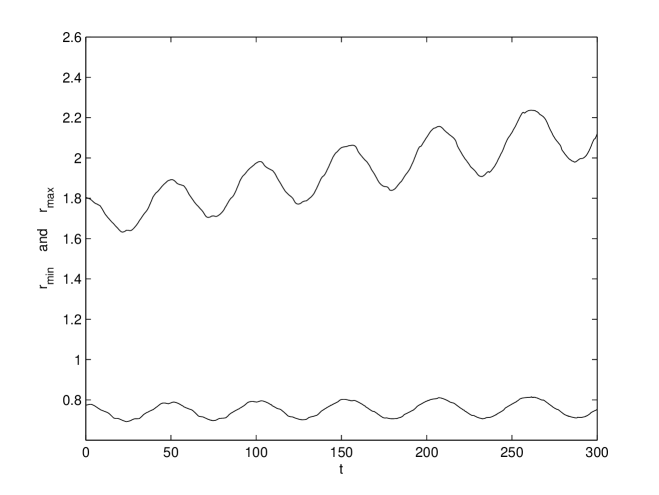
Figure 10: $Z_{c}=0.21,\ E_{b}=0.03,\ A=1.02,\ T=300.0$

The oscillatory behavior with a clear time period is quite striking. We found that all the solutions arising by a small perturbation of a fixed steady state seem to have roughly the same period, independently of $A$. We do at this point venture no interpretation of the slow upward drift of $\alpha(t,0)$ or of $r_{\mathrm{max}}(t)$.

5 Critical phenomena and non-universality

Critical collapse for the Einstein-Vlasov system has previously been studied numerically in [27, 19, 35]. By specifying an initial datum and then varying its amplitude $A,$ a critical value $A_{c}$ of $A$ is found in the sense that if $A>A_{c}$ the evolution of the initial datum will form a trapped surface and collapse to a black hole, and if $A<A_{c}$ no black hole will ever form. In the previous studies referred to above it was stated that the solutions in the subcritical case (i.e. $A<A_{c}$) will disperse to infinity. However, as we saw in the previous section this is not quite true since there are (at least) two possible scenarios: Either the solution will disperse to infinity or it will be bound depending on the sign of the binding energy $e_{b}$. Nevertheless, the value $A_{c}$ separates two distinct behaviors, as was first discovered by Choptuik [7] who studied the Einstein-scalar field system. From his work a new topic developed which goes under the name of critical phenomena, cf. [12] for a review. Two types of matter are distinguished in this context. Vlasov matter is said to be of type I whereas a scalar field and a perfect fluid are of type II. One fundamental difference between matter of type I and type II is that the graph which describes the mass of the black hole (which of course is zero if $A<A_{c}$) as a function of $A$ is discontinuous at $A=A_{c}$ for type I matter, and continuous for type II matter. For type I matter there is thus a mass gap and no possibility to get a black hole with arbitrarily small mass as in the case of type II matter. The characteristic behavior of the critical solution itself has been carefully investigated for type II matter. A lot of evidence has been found that it is self-similar and universal, where the latter property means that it is independent of the initial datum, cf. [12]. For type I matter the general conjecture is that the critical solution is static (and unstable) and universal, see [7]. This conjecture has been investigated in [19] and [35] for Vlasov matter, and evidence that the critical solution is static was found. In these investigations it is also claimed that some support for universality is obtained, but it is concluded that further studies need to be done. From the previous section it is clear that only the static property, and not universality, can be a genuine feature of the critical solution for Vlasov matter. Indeed, by picking $f_{0}=f_{s},$ where $f_{s}$ is the distribution function of an unstable static solution we find $A_{c}=1$ as the critical amplitude and $f_{s}$ as the critical solution. Since there are infinitely many unstable static solutions, and any one will do as critical solution, universality is contradicted. More precisely, within any family of steady states (which we have investigated), specified by some choice of $k$ and $l$ in (23), there are infinitely many unstable ones each of which acts as a critical solution. And the class of steady states of the form (23) is only a small subset of all possible forms of steady states obtainable by the ansatz (22), cf. [25].

If we turn to the other conjectured property, that the critical solution is static, our results strongly support that this is the case. We start from subcritical initial data and tune the amplitude to a very high degree of precision to get $A_{c}.$ We then find that in the evolution the metric coefficients become more or less frozen after some time and stay so during a considerably long time period before the solution starts to drift off outwards. The length of the latter time period depends on how carefully we have calibrated $A_{c}$. By a considerably long time period we mean considerable in comparison to a typical dynamical time scale, e. g. a typical time to form a trapped surface or the typical period time of an oscillation for a bound state. This is further discussed in the next section on the error estimates.

6 The numerical errors

To get an indication of the validity of our simulations we compute at every time step the ADM mass $M(t)$ and the rest mass $M_{0}(t),$ which are conserved along true solutions of the system. We define the errors $e[M]$ and $e[M_{0}]$ by

$$e[M](t)=\frac{|M(t)-M|}{M},\ e[M_{0}](t)=\frac{|M_{0}(t)-M_{0}|}{M_{0}},$$

where $M=M(0)$ and $M_{0}=M_{0}(0)$ are given by the initial datum. As we have explained in previous sections, the evolution of an initial datum will either form a trapped surface and collapse, will be bound and never collapse, or it will disperse to infinity. In the latter two situations the errors in our simulations are remarkably small as can be seen in the table below. On the other hand when a trapped surface has formed a black hole singularity will develop (cf. [11]). The coordinates that we are using are believed to avoid the singularity so that solutions will be regular for all times. However, the solutions become more and more peaked at a certain more or less frozen radius. Of course a very fine grid is needed to resolve such sharp peaks. We are using a fixed grid which does not change with time, and since the solutions get more and more peaked as time goes on our grid is not sufficient after a certain time of the collapse. This results in an essential increase of the errors as seen in Table 5 in the case of collapsing initial data.

$Z_{c}$	$E_{b}$	$A$	TTS	PT	TF	$e[M](TF)$	$e[M_{0}](TF)$
$0.30$	$0.039$	1.01			50	0.00035	0.000036
$0.47$	$0.039$	0.99		60	150	0.0013	0.000023
$1.14$	$-0.080$	0.99			20	0.00015	0.00011
$1.14$	$-0.080$	1.01	3.6		10	0.080	0.040

Table 5: Numerical errors

For each of the simulations in Table 5 about $14\,000$ particles have been used. This gives convenient running times of a few minutes, but one can of course use a much larger number of particles and for certain runnings we have used up to $10^{6}$ particles which gives running times of several hours on a reasonably modern PC. To get an idea of the length of the final running time, $TF,$ we have in the relevant cases included the time when a trapped surface forms, $TTS,$ and the period time, $PT,$ of an oscillation. In the collapsing situation (row $4$) where the errors are of a different magnitude we also computed the error at $t=2*TTS=7.2$ and found $e[M](7.2)=0.024$ and $e[M_{0}](7.2)=0.046,$ in order to get an indication of the growth of the errors. In conclusion, Table 5 clearly demonstrates that we can keep $M$ and $M_{0}$ conserved to a very high precision in the evolution as long as we are not considering collapsing solutions. In the latter case the errors are still very reasonable for a considerable running time compared to the time when a trapped surface forms.

References

- [1] H. Andréasson, The Einstein-Vlasov system/kinetic theory, Living Rev. Relativ. 8 (2005).
- [2] H. Andréasson, On global existence of the spherically symmetric Einstein-Vlasov system in Schwarzschild coordinates. Indiana University Math. J. To appear.
- [3] H. Andréasson, G. Rein, The spherically symmetric Einstein-Vlasov system in maximal areal coordinates. In preparation.
- [4] H. Andréasson, G. Rein, On the steady states of the spherically symmetric Einstein-Vlasov system. In preparation.
- [5] R. Bartnik, J. McKinnon, Particlelike solutions of the Einstein-Yang-Mills equations. Phys. Rev. Lett. 61, 141–143 (1988).
- [6] C. K. Birdsall, A. B. Langdon, Plasma Physics via Computer Simulation. New York: McGraw-Hill 1985
- [7] M. W. Choptuik, Universality and scaling in the gravitational collapse of a scalar field, Phys. Rev. Lett. 70, 9–12 (1993).
- [8] M. W. Choptuik, T. Chmaj, P. Bizoń, Critical behaviour in gravitational collapse of a Yang-Mills field, Phys. Rev. Lett. 77, 424–427 (1996).
- [9] D. Christodoulou, The problem of a self-gravitating scalar field. Commun. Math. Phys. 105, 337–361 (1986).
- [10] D. Christodoulou, A mathematical theory of gravitational collapse. Commun. Math. Phys. 109, 613–647 (1987).
- [11] M. Dafermos, A. D. Rendall, An extension principle for the Einstein-Vlasov system in spherical symmetry, Ann. Henri Poincaré 6, 1137–1155 (2005)
- [12] C. Gundlach, Critical phenomena in gravitational collapse, Living Rev. Relativ. 1999-4, (1999).
- [13] Y. Guo, G. Rein, Stable steady states in stellar dynamics. Arch. Rational Mech. Anal. 147, 225–243 (1999)
- [14] Y. Guo, G. Rein, Existence and stability of Camm type steady states in galactic dynamics. Indiana University Math. J. 48, 1237–1255 (1999)
- [15] Y. Guo, G. Rein, Isotropic steady states in galactic dynamics. Commun. Math. Phys. 219, 607–629 (2001)
- [16] Y. Guo, G. Rein, Stable models of elliptical galaxies. Monthly Not. Royal Astr. Soc. 344, 1396–1406 (2003)
- [17] J. R. Ipser, Relativistic, spherically symmetric star clusters. III. Stability of compact isotropic models, The Astrophys. J. 158, 17–43 (1969)
- [18] E. Malec, N. Ó Murchadha, Optical scalars and singularity avoidance in spherical spacetimes, Phys. Rev. D. 50, 6033–6036 (1994).
- [19] I. Olabarrieta, M. W. Choptuik, Critical phenomena at the threshold of black hole formation for collisionless matter in spherical symmetry, Phys. Rev. D. 65, 024007 (2002).
- [20] G. Rein, The Vlasov-Einstein system with surface symmetry, Habilitationsschrift, Munich, (1995).
- [21] G. Rein, Static shells for the Vlasov-Poisson and Vlasov-Einstein systems. Indiana University Math. J. 48, 335–346 (1999).
- [22] G. Rein, Nonlinear stability of Newtonian galaxies and stars from a mathematical perspective, In: Nonlinear Dynamics in Astronomy and Physics, Annals of the New York Academy of Sciences 1045, 103–119 (2005)
- [23] G. Rein, A. D. Rendall, Global existence of solutions of the spherically symmetric Vlasov-Einstein system with small initial data, Commun. Math. Phys. 150, 561–583 (1992). Erratum: Commun. Math. Phys. 176, 475–478 (1996).
- [24] G. Rein, A. D. Rendall, The Newtonian limit of the spherically symmetric Vlasov-Einstein system, Commun. Math. Phys. 150, 585–591 (1992).
- [25] G. Rein, A. D. Rendall, Compact support of spherically symmetric equilibria in non-relativistic and relativistic galactic dynamics, Math. Proc. Camb. Phil. Soc. 128, 363–380 (2000)
- [26] G. Rein, A. D. Rendall, J. Schaeffer, A regularity theorem for solutions of the spherically symmetric Vlasov-Einstein system, Commun. Math. Phys. 168, 467–478 (1995).
- [27] G. Rein, A. D. Rendall, J. Schaeffer, Critical collapse of collisionless matter—a numerical investigation, Phys. Rev. D 58, 044007 (1998).
- [28] G. Rein, T. Rodewis, Convergence of a particle-in-cell scheme for the spherically symmetric Vlasov-Einstein system, Indiana University Math. J. 52, 821–862 (2003).
- [29] A. D. Rendall, Cosmic censorship and the Vlasov equation. Class. Quantum Grav. 9, L99–L104 (1992).
- [30] A. D. Rendall, Cosmic censorship and the Vlasov equation, Class. Quantum Grav. 9, L99–L104 (1992).
- [31] J. Schaeffer, A class of counterexamples to Jeans’ theorem for the Vlasov-Einstein system, Comm. Math. Phys. 204, 313–327 (1999).
- [32] A. Schulze, Nonlinear stability of stationary shells for the Vlasov-Poisson system. In preparation.
- [33] S. L. Shapiro, S. A. Teukolsky, Relativistic stellar dynamics on the computer. II—Physical Applications, Astrophysical J. 298, 58–79 (1985)
- [34] J. A. Smoller, A. G. Wasserman, S.-T. Yau, J. B. McLeod, Smooth static solutions of the Einstein-Yang-Mills equations. Commun. Math. Phys. 143, 115–147 (1991).
- [35] R. Stevenson, The Spherically Symmetric Collapse of Collisionless Matter, M. Sc. Thesis, The University of British Columbia, (September 1 2005, DRAFT).
- [36] G. Wolansky, Static solutions of the Vlasov-Einstein system, Arch. Rational Mech. Anal. 156 205–230 (2001)
- [37] Ya. B. ZelD́ovich, I. D. Novikov, Relativistic Astrophysics Vol. 1, Chicago: Chicago University Press (1971)
- [38] Ya. B. ZelD́ovich, M. A. Podurets, The evolution of a system of gravitationally interacting point masses, Soviet Astronomy–AJ 9, 742–749 (1965), translated from Astronomicheskii Zhurnal 42, 963–973 (1965)