A Numerical Approach to Space-Time Finite Elements for the Wave Equation

Abstract

We study a space-time finite element approach for the nonhomogeneous wave equation using a continuous time Galerkin method. We present fully implicit examples in $1+1$, $2+1$, and $3+1$ dimensions using linear quadrilateral, hexahedral, and tesseractic elements. Krylov solvers with additive Schwarz preconditioning are used for solving the linear system. We introduce a time decomposition strategy in preconditioning which significantly improves performance when compared with unpreconditioned cases.

I Introduction

Space-time finite elements provide some natural advantages for numerical relativity. With space-time elements, time-varying computational domains are straightforward, higher-order approaches are easily formulated, and both time and spatial domains can be discretized using a single unstructured mesh. However, while continuous Galerkin approaches employing space-time finite elements have found use in many engineering applications Csik , Kim , Idesman , Guddati , Kit , they have not been used in numerical relativity. Recent numerical relativity evolutions using finite elements employ discretization of the space domain and marching in time rather than simultaneous discretization of both space and time domains Sopuerta , Cherubini , Cherubini2 .

We investigate a space-time finite element method similar to French1996 using continuous approximation functions in both space and time to explore its use for numerical relativity simulations. The main purpose of this paper is to present our numerical results. We present a time-parallel preconditioning strategy for use with continuous space-time elements and Krylov solvers, and explore numerical results in $1+1$ dimensions and higher.

Many space-time approaches to the wave equation exist (see Falk , Hughes , French91 , Hulbert ). Our approach is different in that we do not use time slab finite elements, which are continuous in a limited domain of time (the time slab) but discontinuous between neighboring time slabs. Instead, we discretize space and time together for the entire domain using a finite element space which does not discriminate between space and time basis functions and consider iterative solution methods with a time decomposition preconditioner. This approach has advantages for more general finite element spaces and parallelization. In this paper, however, we restrict ourselves to structured space-time finite elements and present the results obtained on a single processor in order to better compare results and performance with other approaches to solving the wave equation.

We consider the following nonhomogeneous wave equation problem with the initial and boundary value problem to find $u({\bf x},t)$ such that

$$\frac{\partial^{2}u}{\partial t^{2}}-\triangle u=f\hskip 4.26773pt {\rm in} \hskip 4.26773pt\Omega\times[0,T],$$ (1)

$$u=u^{0}\hskip 4.26773pt {\rm on} \hskip 4.26773pt\Omega\times\{t=0\},$$

$$u_{t}=v^{0}\hskip 4.26773pt {\rm on} \hskip 4.26773pt\Omega\times\{t=0\},$$

$$u_{n}=0\hskip 4.26773pt {\rm on} \hskip 4.26773pt\partial\Omega\times[0,T],$$

where $\Omega$ is a bounded domain in $R^{d},\,\,d=1,2,3$ and $u_{n}$ is the outward pointing normal derivative. As in French1996 , Eq. (1) is re-written to be first order in time by introducing an auxiliary variable, $v=u_{t}$:

$$\frac{\partial v}{\partial t}-\triangle u=f\hskip 4.26773pt {\rm in} \hskip 4.26773pt\Omega\times[0,T],$$ (2)

$$-\frac{\partial u}{\partial t}+v=0\hskip 4.26773pt {\rm in} \hskip 4.26773pt\Omega\times[0,T],$$

$$u=u^{0}\hskip 4.26773pt {\rm on} \hskip 4.26773pt\Omega\times\{t=0\},$$

$$v=v^{0}\hskip 4.26773pt {\rm on} \hskip 4.26773pt\Omega\times\{t=0\},$$

$$u_{n}=0\hskip 4.26773pt {\rm on} \hskip 4.26773pt\partial\Omega\times[0,T],$$

$$v_{n}=0\hskip 4.26773pt {\rm on} \hskip 4.26773pt\partial\Omega\times[0,T].$$

We use a nonhomogeneous Dirichlet boundary condition on the initial boundary $\Omega\times\{t=0\}$, and a homogeneous Neumann boundary condition for $\partial\Omega\times(0,T]$. No boundary condition is set at $\Omega\times\{t=T\}$ to avoid overspecifying the problem. Consequently, the evolution equations themselves become an effective boundary condition by determining the values for the solution at $\Omega\times\{t=T\}$.

The space $L^{2}(\Omega)$ is defined as the closure of $C^{\infty}(\Omega)$ in the norm,

$$||u||_{L^{2}(\Omega)}=\left(\int_{\Omega}|u|^{2}dx\right)^{1/2}<\infty.$$

The $H^{1}$-seminorm and norm of $u\in H^{1}(\Omega)$ are, respectively,

$$|u|^{2}_{H^{1}(\Omega)}=\int_{\Omega}|\nabla u|^{2}\,dx;\quad||u||^{2}_{H^{1}(\Omega)}=|u|^{2}_{H^{1}(\Omega)}+||u||^{2}_{L^{2}(\Omega)}.$$

We define the Hilbert space $L^{2}([0,T],H^{1}(\Omega))$ by

$$||w||_{L^{2}([0,T],H^{1}(\Omega))}=\Big{(}\,\,\int^{T}_{O}||w(\cdot,t)||^{2}_{H^{1}(\Omega)}\,dt\,\,\Big{)}^{1/2}.$$

For the space-time finite element space of $n=1,2,3$ spatial dimensions, we consider the standard finite element space of $n+1$ dimensions. Therefore our finite element space $V$ is the space of piecewise polynomial functions $\phi:\Omega\times(0,T]\rightarrow R$.

The weak form is to find approximate solutions $\tilde{u},\tilde{v}\in L^{2}([0,T],H^{1}(\Omega))$ such that

$$M\left(\tilde{u},\tilde{v},\phi\right) = 0\hskip 4.26773pt$$ (3)

$$N\left(\tilde{u},\tilde{v},\phi\right) = 0\hskip 4.26773pt\hskip 9.95863pt\forall\phi\in L^{2}([0,T],H^{1}(\Omega)),$$ (4)

where

$$M\left(\tilde{u},\tilde{v},\phi\right) = \int_{\Omega\times[0,T]}\left(\frac{\partial\tilde{v}}{\partial t}\phi+{\bf\nabla}\tilde{u}\cdot{\bf\nabla}\phi-f\phi\right)ds,$$ (5)

$$N\left(\tilde{u},\tilde{v},\phi\right) = \int_{\Omega\times[0,T]}\left(-\frac{\partial\tilde{u}}{\partial t}\phi+\tilde{v}\phi\right)ds.$$ (6)

Motivated by the success of domain decomposition methods for general sparse matrices Toselli:2004:DDM , Sarkis , Cai , we also examine additive Schwarz methods 6wid , 2dry , 6dry , 1cs , Xu with a time decomposition preconditioning strategy. While additive Schwarz preconditioning has been applied to hyperbolic problems before Wu , Cai2 , applying additive Schwarz preconditioning to space-time elements using a time decomposition strategy is unique to this work.

II Numerical Results

In this section we present solutions to the nonhomogeneous wave equation using space-time elements in various dimensions. We use uniform structured meshes to better compare results with other approaches to solving the wave equation. Solutions presented are produced by a single linear solve of the system in Eqs. (3)–(4). All codes presented use PETSc petsc-web-page , petsc-user-ref , petsc-efficient ; the linear solve residuals given (labeled “Final Residuals”) are the absolute residual norms,

$$r=||Ax-b||_{L_{2}}$$ (7)

for the linear system $Ax=b$ where $A$ is the system matrix, $x$ is the solution, and $b$ is the system right hand side vector for both $\tilde{u}$ and $\tilde{v}$. We use the $L_{\infty}$ norm for reporting differences between the analytic and approximate solution:

$$||e||_{L_{\infty}}=\max|e^{i}|,$$ (8)

for vector $e$. For Krylov solve examples, the initial guess given for the solution is always zero.

II.1 $1+1$ Dimensions

For $1+1$ dimensions, we consider the nonhomogeneous wave equation with solution

$$U_{e}\left(x,t\right)=\exp\left[-\left(x-\cos t\right)^{2}\right]$$ (9)

on a domain of $x=\left[-5,5\right]$ and $t=\left[0,10\right]$. We choose the appropriate source term, $f$, in Eq. 1

$$f = -2\,\left(\cos t\right){e^{-\left(x-\cos t\right)^{2}}}\left(2\,\cos^{3}t-4\,x\cos^{2}t+2\,x^{2}\cos t-2\,\cos\,t+x\right),$$ (10)

and initial conditions to produce this test problem solution. Solving this system via LU decomposition with linear rectangular elements we observe the expected second order convergence, shown in Table 1.

$n_{x}$	$n_{t}$	$\|\left(\tilde{u}-U_{e}\right)\|_{L_{\infty}}$	rate
60	60	$2.21\times 10^{-2}$	–
120	120	$5.11\times 10^{-3}$	$2.08$
240	240	$1.26\times 10^{-3}$	$2.01$

Table 1: Convergence using LU decomposition of a space-time element simulation with solution given by Eq. (9). There are $(n_{x}-1)(n_{t}-1)$ total elements in the mesh. The number of nodes in the $x$ and $t$ directions are $n_{x}$ and $n_{t}$, respectively. Using linear elements, we expect second order convergence in the $L_{\infty}$ norm. The convergence rates reported are given by ${\rm rate}=\ln\left(E_{2}/E_{1}\right)/\ln\left(h_{2}/h_{1}\right)$ where $h_{1},h_{2},E_{1},E_{2}$ are the successive quadrilateral lengths and $L_{\infty}$ norms, respectively.

Since scaling with problem size using LU decomposition for a banded matrix is $O\left(Nb^{2}\right)$ – where $N$ is the size of the matrix and $b$ is the bandwidth – LU is entirely inadequate for large problems with space-time elements. Krylov solvers Saad , like GMRES Saad1986 , are much more suitable for such problems.

We tested a variety of solvers and preconditioners available in PETSc petsc-web-page , petsc-user-ref , petsc-efficient for the problem using a $60^{2}$ structured mesh. The results are summarized in Table 2.

Solver Type	Preconditioner	iterations	Final Residual	$\|\left(\tilde{u}-U_{e}\right)\|_{L_{\infty}}$
GMRES	none	5127	$10^{-5}$	$2.20\times 10^{-2}$
GMRES	none	2000	$10^{-2}$	$3.68\times 10^{-1}$
LSQR	–	5000	$10^{-3}$	$2.48\times 10^{-1}$
GMRES	Jacobi	6000	$10^{-2}$	$8.68$
GMRES	Block-Jacobi	1	$10^{15}$	–

Table 2: Various linear solver tests to solve the $1+1$ problem on a $60^{2}$ structured mesh. GMRES performed the best, but required a very large number of iterations. LSQR is similar to a direct method and cannot be preconditioned in PETSc. Jacobi and Block-Jacobi preconditioning made GMRES convergence even worse than unpreconditioned.

While GMRES converges without preconditioning, it requires a high number of iterations to obtain a physically meaningful result. Preconditioning with Jacobi or Block-Jacobi does not improve the convergence rate. However, neither Jacobi nor Block-Jacobi preconditioning offer much flexibility with respect to the geometry of the problem. Additive Schwarz offers more flexibility in preconditioning this hyperbolic problem.

We follow a time decomposition strategy for additive Schwarz, as illustrated in Figure 1. The domain of the problem is split into separate subdomains of time slabs. Each subdomain overlaps the face cells of its neighbors. The much smaller linear system of each subdomain is subsequently solved, either by GMRES or by LU decomposition, and the result used for preconditioning the global system. We respect the original boundary conditions for the subspace interface condition: Dirichlet for $t=\left(t_{n-1}-{\rm overlap}\right)$ and evolution equation determined for $t=\left(t_{n}+{\rm overlap}\right)$ where $t_{n}$ is the $n$-th time decomposition.

Results for time decomposition of a $60^{2}$ mesh are summarized in Table 3.

Solver Type	Preconditioner	# of subdomains	iterations	Final Residual	$\|\left(\tilde{u}-U_{e}\right)\|_{L_{\infty}}$
GMRES	ASM	4	100	$10^{-4}$	$2.15\times 10^{-2}$
GMRES	ASM	4	500	$10^{-5}$	$2.21\times 10^{-2}$
GMRES	ASM	5	200	$10^{-4}$	$2.22\times 10^{-2}$
GMRES	ASM	6	200	$10^{-4}$	$2.50\times 10^{-2}$
GMRES	ASM	10	500	$10^{-4}$	$2.27\times 10^{-2}$
GMRES	ASM	12	500	$10^{-4}$	$2.39\times 10^{-2}$

Table 3: GMRES results using additive Schwarz method (ASM) preconditioning with a time decomposition strategy for the $1+1$ dimension case using a $60^{2}$ structured mesh. The column labeled “Final Residual” gives the absolute residual norm for the linear solve. All the results show significant improvement over the comparable unpreconditioned GMRES case shown in Table 2. Increasing the number of time subdomains generally requires more GMRES iterations to achieve comparable error residuals; however, the preconditioner is potentially faster with more subdomains. Also, the preconditioner would be more scalable in parallel when using more subdomains.

Figure 2 shows plots of the solution after 1, 10, 100, and 500 GMRES iterations for the twelve subdomain additive Schwarz case. Subdomains were defined for this case by equally dividing up the global domain into time slabs consisting of 5 or 6 nodes each in the time direction.

The additive Schwarz preconditioner gives excellent performance compared to GMRES alone and provides a scalable alternative to LU decomposition for large problems. Furthermore, the additive Schwarz preconditioner is already suitable for time-parallel computation; each processor would take a portion of the time subdomain in preconditioning. Spatial domain decomposition could also be explored in connection with time decomposition; however, we restrict our attention to time decomposition here.

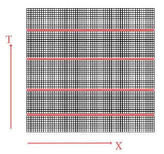
Figure 1: The $60^{2}$ mesh used for the $1+1$ dimension simulations. Here the entire mesh is divided into five subdomains in time for use in preconditioning. The linear systems resulting from each subdomain are solved and the result used for preconditioning the global linear system. The subspace interface condition is the same as for the original boundary conditions: Dirichlet for $t=\left(t_{n-1}-{\rm overlap}\right)$ and evolution equation determined for $t=\left(t_{n}+{\rm overlap}\right)$ where $t_{n}$ is the $n$-th time decomposition. This preconditioner is also time-parallel: each time subdomain could be solved simultaneously on a different processor. Spatial domain decomposition could also be applied, but we only examine time decomposition here.

After 1 iteration	After 10 iterations
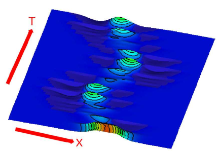
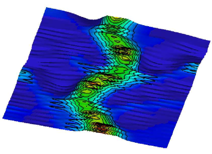
After 100 iterations	After 500 iterations

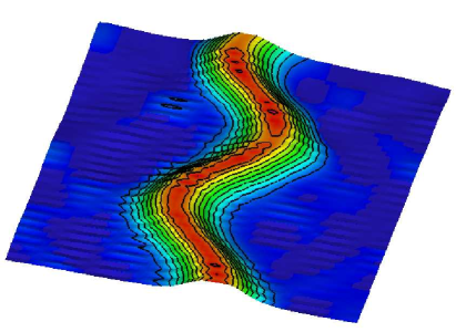
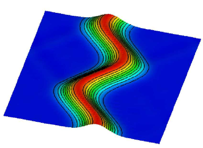
Figure 2: An additive Schwarz preconditioned example using twelve subdomains in time on a $60^{2}$ structured mesh, referenced in Table 3. The plots show the solution after 1,10,100, and 500 GMRES iterations. Unlike time marching methods, the solution is constructed at all times simultaneously. The preconditioner substantially speeds up this process; evidence of the twelve additive Schwarz time subdomains is apparent after the first iteration of GMRES.

II.2 $2+1$ Dimensions

For $2+1$ dimensions, we modify the solution to be

$$U_{e}\left(x,y,t\right)=\exp\left[-\left(x-\cos t\right)^{2}-\left(y+\sin t\right)^{2}\right].$$ (11)

on a domain of $x,y=\left[-4,4\right]$ and $t=\left[0,4\right]$. The linear system is constructed using linear hexahedral elements giving second order convergence for the system.

A time decomposition strategy for preconditioning is also explored in $2+1$. Like the $1+1$ case, employing a time decomposition strategy with additive Schwarz preconditioning significantly improves performance when compared to using GMRES alone or LU decomposition. Table 4 gives a summary of results obtained using a $40\times 40\times 20$ mesh. Performance times given are the solve times obtained on AMD opteron 250 processor with a clock speed of 2.4 GHz using the PETSc timing utility.

Solver Type	Preconditioner	# of subdomains	iterations	Final Residual	$\|\left(\tilde{u}-U_{e}\right)\|_{L_{\infty}}$	Time (sec)
LU	-	-	-	$10^{-14}$	$2.73\times 10^{-2}$	$2.1\times 10^{3}$
GMRES	none	1	3000	$10^{-2}$	$2.10\times 10^{-1}$	$2.8\times 10^{3}$
GMRES	ASM	4	500	$10^{-4}$	$2.92\times 10^{-2}$	$1.5\times 10^{2}$
GMRES	ASM	4	1000	$10^{-5}$	$2.77\times 10^{-2}$	$4.0\times 10^{2}$
GMRES	ASM	5	500	$10^{-4}$	$2.90\times 10^{-2}$	$1.5\times 10^{2}$
GMRES	ASM	5	1000	$10^{-4}$	$2.77\times 10^{-2}$	$4.1\times 10^{2}$

Table 4: Linear solve results for the $2+1$ dimension case using a $40\times 40\times 20$ structured mesh. The column labeled “Final Residual” gives the absolute residual norm for the linear solve. The additive Schwarz preconditioned cases show significant performance gain over the comparable unpreconditioned GMRES case and LU case. The performance times, given in seconds, were obtained using the PETSc timing utility running on an AMD opteron 250 processor. The GMRES simulations required significantly less memory than LU decomposition. Figure 3 shows the solution for the five subdomain ASM case after 10, 50, 100, and 500 GMRES iterations.

GMRES without preconditioning is ineffective for this problem due to the slow convergence rate. As expected, LU decomposition is also ineffective due to poor scaling as the problem size grows. In contrast, GMRES with additive Schwarz method (ASM) preconditioning using a time decomposition strategy is significantly more effective. Figure 3 shows plots of the solution after 10, 50, 100, and 500 GMRES iterations for the five subdomain ASM preconditioned case. As in the $1+1$ cases, the ASM preconditioner is time-parallel: parallelization can be achieved by simultaneously solving each time subdomain on a different processor.

After 10 iterations	After 50 iterations
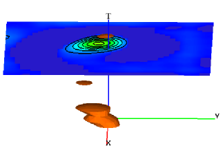
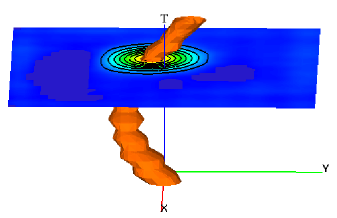
After 100 iterations	After 500 iterations

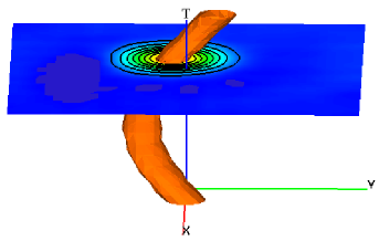
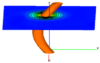
Figure 3: An additive Schwarz preconditioned example in $2+1$ dimensions using five subdomains in time on a $40\times 40\times 20$ structured mesh, referenced in Table 4. The plots show the solution after 10,50,100, and 500 GMRES iterations. The isosurface indicates a surface with value of 0.8, tracking the motion of the pulse in time. A slice of the solution at time 3 is also shown with contour lines on the slice. The vertical axis is the time direction. Like Figure 2 in the $1+1$ dimension case, the solution is constructed at all timesteps at once rather than sequentially solving a single timestep at a time as in time marching methods

.

II.3 $3+1$ Dimensions

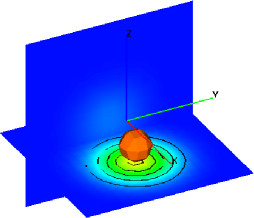
Figure 4: Initial data for $3+1$ simulation in Figure 5.

	Time 1:	Time 3:	Time 5:
10 iterations:
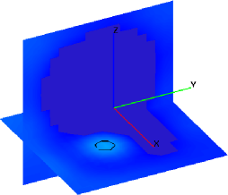
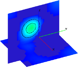
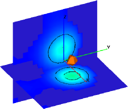
50 iterations:
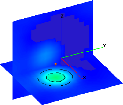
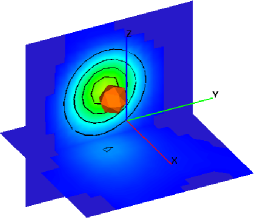
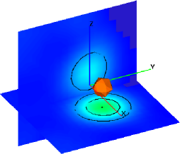
100 iterations:
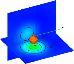
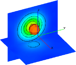
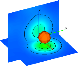
750 iterations:

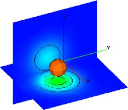
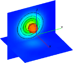
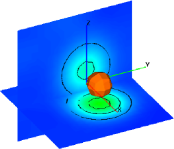
Figure 5: The additive Schwarz preconditioned $3+1$ example using nine subdomains in time on a $18^{4}$ structured mesh referred to in Table 5. The initial data for this simulation is shown in Figure 4. The plots here show the solution, by row, after 10,50,100, and 750 GMRES iterations. The columns indicate the time of the solution: the left column shows the solution at time 1, the middle column shows time 3, and the right column shows time 5. An isosurface with value 0.8 tracks the motion of the pulse. Two spatial planes with contours are also shown: the first on the $x=-1$ plane, and the second on the $z=-1$ plane. Like Figures 2 and 3, the solution is constructed at all times simultaneously. The mesh consists of tesseracts, the higher dimensional analogue of hexahedra. The 3-D datasets shown are time slices from the 4-D mesh.

For $3+1$ dimensions, we select the solution to be

$$U_{e}\left(x,y,z,t\right)=\exp\left[-\left(x-\frac{1}{2}\cos t\right)^{2}-\left(y+\frac{1}{2}\sin t\right)^{2}-\left(z+\frac{1}{2}\cos t\right)^{2}\right].$$ (12)

on a domain of $x,y,z=\left[-2.5,2.5\right]$ and $t=\left[0,5\right]$. The linear system is constructed using linear tesseractic elements consisting of 16 nodes per element, giving second order convergence for the system. Tesseracts are the higher dimensional analogue of hexahedra Mathworld . Table 5 gives a summary of results obtained using a $18^{4}$ mesh.

Solver Type	Preconditioner	# of subdomains	iterations	Final Residual	$\|\left(\tilde{u}-U_{e}\right)\|_{L_{\infty}}$
GMRES	ASM	6	300	$10^{-4}$	$8.13\times 10^{-2}$
GMRES	ASM	9	300	$10^{-3}$	$8.53\times 10^{-2}$
GMRES	ASM	9	600	$10^{-3}$	$8.17\times 10^{-2}$
GMRES	ASM	9	750	$10^{-4}$	$8.15\times 10^{-2}$

Table 5: Linear solve results for the $3+1$ dimension case using an $18^{4}$ structured mesh. The column labeled “Final Residual” gives the absolute residual norm for the linear solve. Unlike the $1+1$ and $2+1$ cases, these $3+1$ examples were only possible on a single processor because of the additive Schwarz preconditioning; both LU decomposition and unpreconditioned GMRES were impractical because of memory limitations or time limitations. These $3+1$ simulations used a mesh composed of linear tesseracts: 16 node 4-D hyperelements. Figure 4 shows the initial data used for these simulations; Figure 5 shows the solution for the nine subdomain ASM case after 10, 50, 100, and 750 GMRES iterations at three times: 1,3, and 5.

Figures 4–5 show plots of the solution at selected time slices; Figure 5 shows the nine subdomain additive Schwarz preconditioned case at 10, 50, 100, and 750 GMRES iterations.

III Conclusions

We have numerically examined space-time finite elements for the nonhomogeneous wave equation, testing several types of linear solvers and preconditioners in several dimensions. The motivation of this study is to explore the performance issues surrounding the use of space-time elements in the context of numerical relativity. Fully unstructured meshes in space and time can greatly simplify issues surrounding time-varying computational domains and space-time mesh refinement, provided that both the domain and refinement are specified a priori. They have also shown promise when the time-varying domain is not known a priori, as in Walhorn and Hansbo . We restricted our attention to those simulations which could be performed on a single processor. Fully implicit examples using a continuous time Galerkin method were presented in $1+1$, $2+1$, and $3+1$ dimensions using linear quadrilateral, hexahedral, and tesseractic elements.

We found that LU decomposition and unpreconditioned GMRES were both capable of solving the linear systems which appear in these space-time element simulations. However, both choices scaled too poorly with respect to problem size to be effective even for moderate size simulations in $3+1$. Standard preconditioners like Jacobi and Block-Jacobi did not improve GMRES performance for the space-time linear systems.

We found that additive Schwarz preconditioning significantly improved GMRES performance. Substantial performance improvements were observed by applying a time decomposition strategy in additive Schwarz preconditioning. The time decomposition strategy consisted of decomposing the global mesh into several smaller time subdomains for use in preconditioning. This preconditioning strategy is also time-parallel: all the time subdomains used in preconditioning can be solved simultaneously on separate processors.

Several improvements upon the additive Schwarz preconditioner remain to be explored. In the experiments presented here, only face cell overlap was examined. Also, no attempt was made to combine time decomposition with spatial domain decomposition even though such a combination would be natural. A study of the optimal interface condition kimn:2005 is another interesting question since the interface condition explored here was physically motivated. Attempts at a parallel implementation of the preconditioner will be forthcoming. The substantial performance benefits of the ASM preconditioner make further study into space-time elements for numerical relativity feasible.

IV Acknowledgements

Early prototyping benefited from two finite element packages: libmesh libmesh and Diffpack diffpack . We also acknowledge helpful discussions with Luis Lehner and Jorge Pullin. This work was supported by the following grants: NSF-PHY-0244335, NSF-PHY-0244299, NSF-INT0204937, and NASA-NAG5-13430.

References

- (1) A. Csik and H. Deconinck. Space-time residual distribution schemes for hyperbolic conservation laws on unstructured linear finite elements. International Journal for Numerical Methods in Fluids, 40(3-4):573 – 581, 2002.
- (2) C.-Y. Kim. On the numerical computation for solving the two-dimensional parabolic equations by space-time finite element method. JSME International Journal, Series B: Fluids and Thermal Engineering, 44(3):434 – 438, 2001.
- (3) A. Idesman, R. Niekamp, and E. Stein. Finite elements in space and time for generalized viscoelastic maxwell model. Computational Mechanics, 27(1):49 – 60, 2001.
- (4) M.N. Guddati and J.L. Tassoulas. Space-time finite elements for the analysis of transient wave propagation in unbounded layered media. International Journal of Solids and Structures, 36(31-32):4699 – 4723, 1999.
- (5) K.M. Kit and J.M. Schultz. Space-time finite element model to study the influence of interfacial kinetics and diffusion on crystallization kinetics. International Journal for Numerical Methods in Engineering, 40(14):2679 – 2692, 1997.
- (6) Carlos Sopuerta and Pablo Laguna. A finite element computation of the gravitational radiation emitted by a point-like object orbiting a non-rotating black hole. arXiv:gr-qc/0512028, 2005.
- (7) C. Cherubini and S. Filippi. Using FEMLAB for gravitational problems: numerical simulations for all. arXiv:gr-qc/0509099, 2005.
- (8) C. Cherubini, F. Federici, S. Succi, and M.P. Tosi. Excised acoustic black holes: The scattering problem in the time domain. Phys. Rev. D, 72:084016, 2005.
- (9) Donald A. French and Todd E. Peterson. A continuous space-time finite element method for the wave equation. Mathematics of Computation, 65:491–506, 1996.
- (10) R. Falk and G. Richter. Explicit finite element methods for linear hyperbolic systems. In B. Cockburn, G.E. Karniadakis, and C.-W. Shu, editors, Discontinuous Galerkin Methods, Lecture Notes in Computational Science and Engineering, pages 209–219. Springer-Verlag, 2000.
- (11) G. Hulbert and T. Hughes. Space-time finite element methods for second-order hyperbolic equations. Comput. Methods Appl. Mech. Engrg., 84:327–348, 1990.
- (12) D. French. A space-time finite element method for the wave equation. Comput. Methods Appl. Mech. Engrg., 107:145–157, 1993.
- (13) G. Hulbert. Space-time finite element methods. In Franca, Tezduyar, and Masud, editors, Finite Element Methods: 1970’s and Beyond, pages 116–123, 2004.
- (14) Andrea Toselli and Olof Widlund. Domain Decomposition Methods - Algorithms and Theory, volume 34 of Springer Series in Computational Mathematics. Springer, 2004.
- (15) Marcus Sarkis. Domain decomposition methods: Schwarz methods. In Applied methematics and scientific computing (Dubrovnik, 2001), pages 3–29. Kluwer/Plenum, New York, 2003.
- (16) Xiao-Chuan Cai and Yousef Saad. Overlapping domain decomposition algorithms for general sparse matrices. Numer. Linear Algebra Appl., 3(3):221–237, 1996.
- (17) Maksymilian Dryja and Olof B. Widlund. An additive variant of the Schwarz alternating method for the case of many subregions. Technical Report 339, Department of Computer Science, Courant Institute, 1987.
- (18) Maksymilian Dryja. An additive Schwarz algorithm for two- and three-dimensional finite element elliptic problems. In Tony Chan, Roland Glowinski, Jacques Périaux, and Olof Widlund, editors, Domain Decomposition Methods, pages 168–172, Philadelphia, PA, 1989. SIAM.
- (19) Maksymilian Dryja and Olof B. Widlund. Additive Schwarz methods for elliptic finite element problems in three dimensions. In David E. Keyes, Tony F. Chan, Gérard A. Meurant, Jeffrey S. Scroggs, and Robert G. Voigt, editors, Fifth International Symposium on Domain Decomposition Methods for Partial Differential Equations, pages 3–18, Philadelphia, PA, 1992. SIAM.
- (20) Xiao-Chuan Cai and Marcus Sarkis. A restricted additive Schwarz preconditioner for general sparse linear systems. SIAM Journal on Scientific Computing, 21:239–247, 1999.
- (21) J. Xu. Iterative methods by space decomposition and subspace correction. SIAM Review, 34(4):581–613, 1992.
- (22) Yunhai Wu, Xiao-Chuan Cai, and David E. Keyes. Additive Schwarz methods for hyperbolic equations. In Domain decomposition methods, 10 (Boulder, CO, 1997), volume 218 of Contemp. Math., pages 468–476. Amer. Math. Soc., Providence, RI, 1998.
- (23) Xiao-Chuan Cai, William D. Gropp, David E. Keyes, Robin G. Melvin, and David P. Young. Parallel Newton–Krylov–Schwarz algorithms for the transonic full potential equation. SIAM Journal on Scientific Computing, 19(1):246–265, 1998.
- (24) Satish Balay, Kris Buschelman, William D. Gropp, Dinesh Kaushik, Matthew G. Knepley, Lois Curfman McInnes, Barry F. Smith, and Hong Zhang. PETSc Web page, 2001. http://www.mcs.anl.gov/petsc.
- (25) Satish Balay, Kris Buschelman, Victor Eijkhout, William D. Gropp, Dinesh Kaushik, Matthew G. Knepley, Lois Curfman McInnes, Barry F. Smith, and Hong Zhang. PETSc users manual. Technical Report ANL-95/11 - Revision 2.1.5, Argonne National Laboratory, 2004.
- (26) Satish Balay, William D. Gropp, Lois Curfman McInnes, and Barry F. Smith. Efficient management of parallelism in object oriented numerical software libraries. In E. Arge, A. M. Bruaset, and H. P. Langtangen, editors, Modern Software Tools in Scientific Computing, pages 163–202. Birkhäuser Press, 1997.
- (27) Y. Saad. Iterative methods for sparse linear systems. SIAM, 2003. 2nd Ed.
- (28) Y. Saad and M. Schultz. GMRES: A generalized minimal residual algorithm for solving nonsymmetric linear systems. SIAM J. Sci. Statist. Comput., 7:856–869, 1986.
- (29) Eric W. Weisstein. “Tesseract” from MathWorld – a wolfram web resource. http://mathworld.wolfram.com/Tesseract.html.
- (30) E. Walhorn, A. Kolke, B. Hubner, and D. Dinkler. Fluid-structure coupling within a monolithic model involving free surface flows. Computers and Structures, 83(25-26):2100 – 2111, 2005.
- (31) Peter Hansbo, Joakim Hermansson, and Thomas Svedberg. Nitsche’s method combined with space-time finite elements for ale fluid-structure interaction problems. Computer Methods in Applied Mechanics and Engineering, 193:4195 – 4206, 2004.
- (32) Jung-Han Kimn. A convergence theory for an overlapping Schwarz algorithm using discontinuous iterates. Numer. Math., 100(1):117–139, 2005.
- (33) http://libmesh.sourceforge.net.
- (34) http://www.diffpack.com.