Theoretical foundations for on-ground tests of LISA PathFinder thermal diagnostics

Abstract

This paper reports on the methods and results of a theoretical analysis to design an insulator which must provide a thermally quiet environment to test on ground delicate temperature sensors and associated electronics. These will fly on board ESA’s LISA Pathfinder (LPF) mission as part of the thermal diagnostics subsystem of the LISA Test-flight Package (LTP). We evaluate the heat transfer function (in frequency domain) of a central body of good thermal conductivity surrounded by a layer of a very poorly conducting substrate. This is applied to assess the materials and dimensions necessary to meet temperature stability requirements in the metal core, where sensors will be implanted for test. The analysis is extended to evaluate the losses caused by heat leakage through connecting wires, linking the sensors with the electronics in a box outside the insulator. The results indicate that, in spite of the very demanding stability conditions, a sphere of outer diameter of the order one metre is sufficient.

1 Introduction

LISA Pathfinder (LPF) is an ESA mission, whose main objective is to put to test critical parts of LISA (Laser Interferometer Space Antenna), the first space borne gravitational wave (GW) observatory [1]. The science module on board LPF is the LISA Test-flight Package (LTP) [2], which basically consists in two test masses in nominally perfect geodesic motion (free fall), and a laser metrology system, which reports on residual deviations of the test masses’ actual motion from the ideal free fall, to a given level of accuracy [3].

In order to ensure that the test masses are not deviated from their geodesic trajectories by external (non-gravitational) agents, a so called Gravitational Reference System (GRS) is used [4]. This consists in position sensors for the masses which send signals to a set of micro-thrusters; the latter take care of correcting as necessary the spacecraft trajectory, so that at least one of the test masses remains centred relative to the spacecraft at all times. The combination of the GRS plus the actuators is known as drag-free subsystem.

The drag-free is of course a central component of LISA, and needs to be operated at extremely demanding levels of accuracy. The laser metrology system should then be sufficiently precise to measure relative test mass deviations. The overall level of noise acceptable for LISA is defined in terms of rms acceleration spectral density, and has been set to

$$S_{a,{\rm LISA}}^{1/2}(\omega)\leq 3\!\times\!10^{-15}\,\left[1+\left(\frac{\omega/2\pi}{3\ {\rm mHz}}\right)^{\!\!2}\right]\,{\rm m}\,{\rm s}^{-2}/\sqrt{\rm Hz}$$ (1)

in the frequency range $\quad 10^{-4}\,{\rm Hz}\leq\omega/2\pi\leq 10^{-3}\,{\rm Hz}$. This is equivalent to $S_{h}^{1/2}$ $\sim$ 4$\times$10^-21 Hz^-1/2, with the same frequency dependence.

Because LPF is a technological mission, aimed to assess the feasibility of LISA, its ultimate goal has been relaxed to [5]

$$S_{a,{\rm LPF}}^{1/2}(\omega)\leq 3\!\times\!10^{-14}\,\left[1+\left(\frac{\omega/2\pi}{3\ {\rm mHz}}\right)^{\!\!2}\right]\,{\rm m}\,{\rm s}^{-2}/\sqrt{\rm Hz}$$ (2)

in the frequency range $1\,{\rm mHz}\leq\omega/2\pi\leq 30\,{\rm mHz}$, i.e., one order of magnitude less demanding, both in noise amplitude and in frequency band.

Equation (2) gives the global noise budget. This is naturally made up of contributions from different perturbative agents, such as temperature and magnetic field fluctuations, GRS and interferometer noise, etc. As a general rule, a requirement on the magnitude of each of the various perturbing factors is set at a 10 % fraction of the total. In the case of temperature fluctuations, this is equivalent to

$$S_{T}^{1/2}(\omega)\leq 10^{-4}\,{\rm K}/\sqrt{\rm Hz}\ ,\quad 1\,{\rm mHz}\leq\omega/2\pi\leq 30\,{\rm mHz}$$ (3)

Because temperature stability is important, a decision has been taken to place high precision thermometers in several strategic spots across the LTP—as part of what is called Diagnostics Subsystem [6] . Such high precision temperature measurements will be useful to identify the fraction of the total system noise which is due to thermal fluctuations only, and this will in turn provide important debugging information to assess the performance of the LTP.

1.1 Temperature measurements

If the temperature gauges are to be sensitive to fluctuations at the level given by (3) then clearly the entire measuring device should be less noisy, typically by a factor of 10. This means that such device, which includes both the sensors and the associated electronics, can generate a maximum level of noise of

$$S_{T,{\rm sensor}}^{1/2}(\omega)\leq 10^{-5}\,{\rm K}/\sqrt{\rm Hz}\ ,\quad 1\,{\rm mHz}\leq\omega/2\pi\leq 30\,{\rm mHz}$$ (4)

Research work is currently being conducted at IEEC (Barcelona, Spain) to identify the appropriate sensors and design the better suited front end electronics. But the prototype system needs of course to be tested for compliance with equation (4). Thus, in order to do a meaningful test, the system must be sufficiently thermally isolated that the observed fluctuations in the readout data can be attributed solely to sensor noise, rather than to a combination of it with real ambient temperature fluctuations. This means temperature fluctiations in the thermomters’ placements should again be at least one order of magnitude below the target sensitivity, equation (4), or

$$S_{T,{\rm testbed}}^{1/2}(\omega)\leq 10^{-6}\,{\rm K}/\sqrt{\rm Hz}\ ,\quad 1\,{\rm mHz}\leq\omega/2\pi\leq 30\,{\rm mHz}$$ (5)

It turns out that 10${}^{-6}\,{\rm K}/\sqrt{\rm Hz}$ is a truly demanding temperature stability, orders of magnitude beyond the capabilities of normal thermally regulated rooms. We thus need to design a specific thermal insulator to shield the sensors from ambient temperature fluctuations during the test process.

In the ensuing pages we describe in detail the insulator design. It is extremely important to stress at this point that the performance of the insulator, i.e., its ability to screen out ambient temperature fluctuations, cannot be checked experimentally, at least under working thermal conditions in the laboratory. This is because, by definition, the insulator is the tool to check the sensing instruments, not viceversa: we need to rely on the results of theoretical argumentation to make a decission on which is the appropriate thermal insulator for our purposes. An experimental verification of the model is only thinkable under much more extreme conditions, where external temperature fluctuations are orders of magnitude higher than the ones which will be met during the test.

2 Thermal insulator design concept

The idea of the insulator design is displayed in figure 1: an interior metal core of good thermal conductivity is surrounded by a thick layer of a poorly conductive material. The inner block ensures thermal stability of the sensors attached to it, while the surrounding substrate efficiently shields it from external temperature fluctuations in the laboratory ambient. We propose a spherical shape for the sake of simplicity of the mathematical analysis, even though this will be eventually changed to cubic in the actual experimental device due to practical feasibility issues.

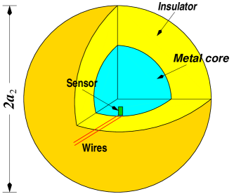
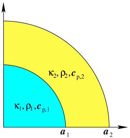
Figure 1: Thermal insulator design concept. Left: 3D diagramme, including sensor placement principle. Right: cut view, with notation convention dictionary.

2.1 Mathematical model

The basic assumption of the mathematical analysis we shall present is that heat flows from the interior of the insulator to the air outside, and from the latter to the interior of the insulator, only by thermal conduction. This is a very realistic hypothesis in the context of the experiment, as radiation mechanisms are certainly negligible and convection should not play any significant role, either, since the entire body is solid, and temperature fluctuations will be small at all times anyway.

Let then $T({\bf x},t)$ be the temperature at time $t\/$ of a point positioned at vector x relative to the centre of the sphere. $T({\bf x},t)$ thus satisfies Fourier’s partial differential equation [7]

$$\rho c_{\rm p}\,\frac{\partial}{\partial t}T({\bf x},t)=\nabla\cdot\left[\kappa\nabla T({\bf x},t)\right]$$ (6)

where $\rho$, $c_{\rm p}$ and $\kappa$ are the density, specific heat and thermal conductivity, respectively, of the substrate. We shall assume these are uniform values within each of the two materials making up the insulating body, with abrupt changes in the interface. We can thus represent them as discontinuous functions of the radial coordinate, as follows:

$$\rho,c_{\rm p},\kappa({\bf x})=\left\{\begin{array}[]{ll}\rho_{1},c_{{\rm p}1},\kappa_{1}&{\rm if}\ \ 0\leq r<a_{1}\\ \rho_{2},c_{{\rm p}2},\kappa_{2}&{\rm if}\ \ a_{1}\leq r<a_{2}\end{array}\right.$$ (7)

with $r\/$ $\equiv$ $|{\bf x}|$. Initial and boundary conditions are the following:

$$T({\bf x},t=0)=0\ ,\quad T(r=a_{2},t)=T_{0}(\theta,\varphi;t)$$ (8)

where $\theta\/$ and $\varphi\/$ are spherical angles which define positions on the sphere’s surface. The boundary temperature can be expediently expressed as a multipole expansion:

$$T_{0}(\theta,\varphi;t)=\sum_{lm}\,b_{lm}(t)\,Y_{lm}(\theta,\varphi)$$ (9)

where $Y_{lm}(\theta,\varphi)$ are spherical harmonics, and $b_{lm}(t)$ are boundary multipole temperature components.

In practice, the boundary temperature will be randomly fluctuating, therefore $b_{lm}(t)$ will be considered stochastic functions of time. We shall also reasonably assume them to be stationary Gaussian noise processes with known spectral densities, $S_{lm}(\omega)$.

As shown in the appendix, the frequency analysis of this problem leads to a transfer function expression of the temperature inside the body:

$$\tilde{T}({\bf x},\omega)=\sum_{lm}\,H_{lm}({\bf x},\omega)\,\tilde{b}_{lm}(\omega)$$ (10)

where tildes ( $\tilde{}$ ) stand for Fourier transforms, e.g.,

$$\tilde{T}({\bf x},\omega)\equiv\int_{-\infty}^{\infty}\,T({\bf x},t)\,e^{-i\omega t}\,dt$$ (11)

etc. If we make the further assumption that different multipole temperature fluctuations at the boundary are uncorrelated, i.e.,

$$\langle\tilde{b}^{*}_{l^{\prime}m^{\prime}}(\omega)\,\tilde{b}_{lm}(\omega)\rangle=S_{lm}(\omega)\,\delta_{l^{\prime}l}\,\delta_{m^{\prime}m}$$ (12)

then the spectral density of fluctuations at any given point inside the insulating body is given by

$$S_{T}({\bf x},\omega)=\sum_{lm}\,\left|H_{lm}({\bf x},\omega)\right|^{2}\,S_{lm}(\omega)$$ (13)

It is ultimately the spectral density $S_{T}({\bf x},\omega)$ which has to comply with the requirement expressed by equation (4). Based on knowledge (by direct measurement) of ambient laboratory temperature fluctuations, equation (13) will provide the guidelines, as regards materials and dimensions, for the actual design of a suitable insulator jig.

3 Homogeneous boundary conditions

Thermal conditions in the laboratory are rather homogeneous. This means that the boundary temperature fluctuations will be in practice essentially independent of the angles $\theta\/$ and $\varphi$, i.e.,

$$T_{0}(\theta,\varphi;t)=B(t)$$ (14)

and consequently the generic expansion equation (9) includes only the monopole term, hence

$$b_{00}(t)=\sqrt{4\pi}\,B(t)$$ (15)

The temperature $T({\bf x},\omega)$ in this case will only depend on radial depth, $r$, therefore,

$$\tilde{T}(r,\omega)=H(r,\omega)\,\tilde{B}(\omega)$$ (16)

with $H(r,\omega)$ $\equiv$ $\sqrt{4\pi}\,H_{00}({\bf x},\omega)$. According to equation (47) of the Appendix, this is

$$H(r,\omega)=\left\{\begin{array}[]{ll}\xi_{0}(\omega)\,j_{0}(\gamma_{1}r)\ ,&0\leq r\leq a_{1}\\[10.00002pt] \eta_{0}(\omega)\,j_{0}(\gamma_{2}r)+\zeta_{0}(\omega)\,y_{0}(\gamma_{2}r)\ ,&a_{1}\leq r\leq a_{2}\end{array}\right.$$ (17)

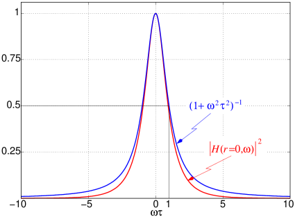
Figure 2: Frequency response at the centre ($r\/$ = 0) of a spherical thermal insulator —as given in equation (17)—, along with the frequency response of a low-pass filter of order one and same frequency cut-off, $\omega_{\rm cut-off}$ = $1/\tau$.

This is a low-pass filter transfer function —even though the cumbersome frequency dependencies involved in the expressions above do not make it immediately obvious. A plot of the square modulus of $H(r,\omega)$ is shown in figure 2 for $r\/$ = 0 (red curve). The figure also shows a low-pass filter of the first order with the same frequency cut-off, $|H_{\rm 1st\ order}(\omega)|^{2}$ = $(1+\omega^{2}\tau^{2})^{-1}$, for conceptual comparison (blue curve).

The most salient feature emerging out of the plot is the stronger drop in $H(r,\omega)$ at the high frequency tails. The latter can be easily assessed in quantitative detail, and the result is

$$|H(0,\omega)|\sim\omega\tau\,e^{-\sqrt{\omega\tau}}$$ (18)

where $\tau$ is the filter’s time constant —a complicated function of the insulator’s physical and geometric properties, to be discussed below.

As already mentioned in the Introduction section, to test the temperature sensors and electronics we need a very strong noise suppression factor in the LTP frequency band. A look at figure 2 readily shows that high damping factors require such frequency band to lie in the filter’s tails. The thermal insulator should therefore be designed in such a way that its time constant $\tau\/$ be sufficiently large to ensure that the LTP frequencies are high enough compared to 1/$\tau\/$. The exponential drop in the transfer function shown by equation (18) makes the filter actually feasible with reasonable dimensions.

4 Numerical analysis

In this section we consider the application of the above formalism to obtain practically useful numbers for the actual implementation of a real insulator device which complies with the needs of our experiment.

First of all, a selection of an aluminum core surrounded by a layer of polyurethane was made. Aluminum is a good heat conductor and is easy to work with in the laboratory; polyurethane is a good insulator and is also convenient to handle, as it can be foamed to any desired shape from canned liquid. Other alternatives are certainly possible, but this appears sufficiently good and we shall therefore only make reference to this specific one.

The relevant physical properties of aluminium and polyurethane are specified in table 1.

	Density	Specific heat	Thermal conductivity
	$\rho$ (kg m-3)	$c_{\rm p}$ (J kg-1 K-1)	$\kappa$ (W m-1 K-1)
Aluminum	2700	900	250
Polyurethane	35	1000	0.04

Table 1: Density, specific heat and thermal conductivity of aluminium and polyurethane. Units are given in the International System.

Figure 3 plots the amplitude damping coefficient of the insulator block, $|H(r,\omega)|$, at the lower end of the LTP frequency band, i.e., 1 mHz, and at the interface position, $r\/$ = $a_{1}$. Each of the curves corresponds to a fixed value of the latter, and is represented as a function of the outer radius of the insulator. This choice is useful because the sensors are implanted for test on the surface of the aluminium core, and also because at higher frequencies thermal damping is stronger. So in practice the actual damping power of the device will be the one plotted, and better at the higher frequencies in the measuring bandwidth. The figure clearly shows that the assymptotic regime of equation (18) is quite early established.

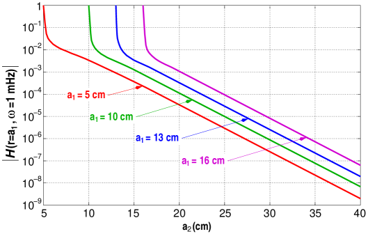
Figure 3: Amplitude damping factor on the interface between aluminium and polyurethane at 1 mHz, for various sizes of the insulating device.

The choice of dimensions for the insulating body must of course ensure that the minimum requirement, equation (5) is met. For this, a primary consideration is the size of the ambient temperature fluctuations in the site where the experiment is made. Dedicated measurements in our laboratory showed that

$$S_{T,{\rm ambient}}^{1/2}(\omega)\sim 10^{-1}\,{\rm K}/\sqrt{\rm Hz}\ ,\quad 1\,{\rm mHz}\leq\omega/2\pi\leq 30\,{\rm mHz}$$ (19)

We therefore need to implement a device such that $|H(a_{1},\omega)|$ $\leq$ 10^-5 throughout the measuring bandwidth (MBW). Suitable dimensions can then be readily read off figure 3, and various alternatives are possible, as seen. Before making a decission, however, we need to make an additional estimate of the heat leakage down the electric wires which connect the temperature sensors with the elctronics, which lies of course outside the insulator. We come to this next.

4.1 Heat leakage through connecting wires

We use a simple model, consisting in assuming the connecting wires behave as straight metallic rods which connect the central aluminum core with the electronics, placed in the external laboratory ambient. Because the polyurethane provides a very stable insulation, we can neglect the lateral flux, hence only a unidimensional heat flow needs to be considered. For this, the following equation relates the heat flux to the temperature difference between the two wires’ edges:

$$\dot{Q}(t)=\kappa_{\rm wire}\,\frac{\pi R_{\rm wire}^{2}}{\ell_{\rm wire}}\;[T(a_{2},t)-T(a_{1},t)]$$ (20)

where $\kappa_{\rm wire}$ is the thermal conductivity of the wire, $R_{\rm wire}$ its transverse radius, and $\ell_{\rm wire}$ its length inside the polyurethane layer.

On the other hand, the heat flux results in temperature variations in the metal core, given by

$$\dot{Q}(t)=\rho_{1}c_{{\rm p}1}V_{1}\,\frac{\partial T}{\partial t}(a_{1},t)$$ (21)

where $V_{1}$ = $4\pi a_{1}^{3}/3$ is the volume of the metal core. Equating the above expressions we find

$$\kappa_{\rm wire}\,\frac{\pi R_{\rm wire}^{2}}{\ell_{\rm wire}}\;[T(a_{2},t)-T(a_{1},t)]=\rho_{1}c_{{\rm p}1}V_{1}\,\frac{\partial T}{\partial t}(a_{1},t)$$ (22)

For fluctuating temperatures, we can now obtain the relationship between the spectral density at the aluminium core and the ambient, due to heat conduction along the wire:

$$S_{T,{\rm wire}}^{1/2}(a_{1},\omega)=|H_{\rm wire}(\omega)|\,S_{T,{\rm ambient}}^{1/2}(\omega)$$ (23)

where

$$|H_{\rm wire}(\omega)|\simeq\frac{\pi}{\omega}\,\frac{\kappa_{\rm wire}\,R_{\rm wire}^{2}}{\rho_{1}c_{{\rm p}1}V_{1}\,\ell_{\rm wire}}$$ (24)

and where the approximation has been made that the temperature fluctuations at the inner end of the wire are much smaller than those at the outer end, due to the presence of the polyurethane layer.

In practice, there will be several sensors for test inside the insulator. Under the hypothesis made that no lateral heat flux is relevant, the transfer function for a bundle of $N\/$ of wires is, at most, $N\/$ times that of a single wire. Thus,

$$|H_{N{\rm wires}}(\omega)|=\frac{3N}{\omega/2\pi}\,\frac{\kappa_{\rm wire}\,R_{\rm wire}^{2}}{8\pi\rho_{1}c_{{\rm p}1}a_{1}^{3}\,\ell_{\rm wire}}$$ (25)

Let us consider numerical values in this expression. We use thin copper wires ($\kappa_{\rm Cu}$ = 401 Wm^-1K^-1) of radius $R_{\rm wire}$ = 0.1 mm, and assume some fiducial parameters for the size of the aluminium core, $a_{1}$, the wire length, $\ell_{\rm wire}$, the number of connecting wires, $N$, and the frequency, $\omega/2\pi$. The following obtains:

$$|H_{N{\rm wires}}(\omega)|=1.1\times 10^{-5}\,\left(\frac{N}{30}\right)\!\left(\frac{a_{1}}{13\ {\rm cm}}\right)^{\!-3}\!\left(\frac{\ell_{\rm wire}}{25\ {\rm cm}}\right)^{\!-1}\!\left(\frac{\omega/2\pi}{1\ {\rm mHz}}\right)^{\!-1}$$ (26)

This result indicates that, for laboratory fluctuations in the level of equation (19), leakage through wiring causes fluctuations in the temperature sensors of about 10^-6 K/$\sqrt{\rm Hz}$, equation (23), which is compliant with the requirement of stability of equation (5). The most sensitive parameter in the above expression is the size of the metal core, and this determines the need to make it somewhat large. The length of the wires has been taken to be 25 cm, but this does not necessarily mean we need $a_{2}$ = 38 cm (assuming the radius of the aluminum core is $a_{1}$ = 13 cm), because the wires can be partly wound inside the polyurethane layer to further protect the system against leakage. In fact, this wire lengthening is an easy way to improve attenuation.

As regards frequency dependence, compliance is guaranteed in the entire MBW if it is at its lower end: indeed, not only $|H_{\rm wire}(\omega)|$ decreases as $\omega^{-1}$, also ambient noise fluctuations drop below 10^-1 K/$\sqrt{\rm Hz}$ at higher frequencies.

5 Conclusions

Temperature fluctuation measurement is very demanding in the LTP, and subsequently LISA, as reflected by equation (4). Accordingly, very delicate sensor and associated electronics must be designed, and of course tested in ground before boarding.

However, even the best laboratory conditions are orders of magnitude worse than the above requirement, so meaningful tests of the temperature sensing system cannot be tested without suitably screening the sensors from ambient temperature fluctuations. We have addressed how this can be accomplished by means of an insulating system consisting of a central metallic core surrounded by a thick layer of a very poorly conducting material. The latter provides good thermal insulation, while the central core, having a large thermal inertia, ensures stability of the sensors’ environemnt. The choice of materials is flexible, so aluminium and polyurethane, which are easily available in the market, has been adopted. Thereafter, the dimensions need to be fixed.

The appropriate sensors for the needs are temperature sensitive resistors, more specifically thermistors —also known as NTCs. It appears that, because these sensors need to be wired to external electronics, heat leakage through such wires is an effect which needs to be quantitatively assessed to prevent losses. We have analysed this problem, and concluded that it strongly depends on the central metallic core size, and imposes that it be somewhat large.

Laboratory ambient temperature fluctuations, determined by dedicated in situ measurements, are of the order of 10^-1 K/$\sqrt{\rm Hz}$ at 1 mHz, and dropping at higher frequencies within the MBW. The required stability conditions at the sensors, attached at the core’s surface, thus need an attenuation factor of 10^-5, or better. Our analysis determines that a central aluminium core of 13 cm of radius, surrounded by a concentric layer of polyurethane 15–20 cm thick, comfortably provides the needed thermal screening which guarantees a meaningful test of the sensors’ performance.

The results of this paper are based on modelling. Because our aim is to produce a very stable thermal environment for the temperature sensors, we cannot check experimentally the correctness of our conclusions. We must instead rely on the validity of the hypotheses made —essentially that heat only flows by thermal conduction— and on the underlying physical laws which govern heat conduction. Even though there is good reason to believe that both are sufficiently accurate, unexpected behaviour e.g. at the interface between the metal core and the insulator, may partly distort the results. Direct measurements with very large temperature gradients applied across the insulating device are envisaged, and will be reported elsewhere as an auxiliary independent test of the model.

Appendix A Thermal insulator frequency response functions

Here we present some mathematical details of the solution to the Fourier problem, equations (6)-(9). We first of all Fourier transform equations (6) and (9):

$$i\omega\,\rho c_{\rm p}\,\tilde{T}({\bf x},\omega)=\nabla\cdot\left[\kappa\nabla\tilde{T}({\bf x},\omega)\right]$$ (27)

$$\tilde{T}_{0}(\theta,\varphi;\omega)=\sum_{l=0}^{\infty}\sum_{m=-l}^{l}\,\tilde{b}_{lm}(\omega)\,Y_{lm}(\theta,\varphi)$$ (28)

Equation (27) can be recast in the form

$$\left(\nabla^{2}+\gamma_{1}^{2}\right)\,\tilde{T}({\bf x},\omega)=0\ ,\quad 0\leq r\leq a_{1}$$ (29)

$$\left(\nabla^{2}+\gamma_{2}^{2}\right)\,\tilde{T}({\bf x},\omega)=0\ ,\quad a_{1}\leq r\leq a_{2}$$ (30)

where $r\/$ $\equiv$ $|{\bf x}|$, and

$$\gamma_{1}^{2}\equiv-i\omega\,\frac{\rho_{1}c_{\rm p,1}}{\kappa_{1}}\ ,\quad\gamma_{2}^{2}\equiv-i\omega\,\frac{\rho_{2}c_{\rm p,2}}{\kappa_{2}}$$ (31)

To these, matching conditions at the interface and boundary conditions must be added:

$$\tilde{T}(r=a_{1}-0,\omega)=\tilde{T}(r=a_{1}+0,\omega)$$ (32)

$$\kappa_{1}\,\frac{\partial\tilde{T}}{\partial r}(r=a_{1}-0,\omega)=\kappa_{2}\,\frac{\partial\tilde{T}}{\partial r}(r=a_{1}+0,\omega)$$ (33)

$$\tilde{T}(r=a_{2},\omega)=\tilde{T}_{0}(\theta,\varphi;\omega)$$ (34)

Equations (29) and (30) are of the Helmholtz kind. Their solutions are thus respectively given by

$$\tilde{T}({\bf x},\omega)=\left\{\begin{array}[]{ll}\displaystyle\sum_{lm}\,A_{lm}(\omega)\,j_{l}(\gamma_{1}r)\,Y_{lm}(\theta,\varphi)\ ,&0\leq r\leq a_{1}\\[16.99998pt] \displaystyle\sum_{lm}\,\left[C_{lm}(\omega)\,j_{l}(\gamma_{2}r)+D_{lm}(\omega)\,y_{l}(\gamma_{2}r)\,\right]\,Y_{lm}(\theta,\varphi)\ ,&a_{1}\leq r\leq a_{2}\end{array}\right.$$ (35)

where $j_{l}\/$ and $y_{l}\/$ are spherical Bessel functions [8],

$$j_{l}(z)=z^{l}\,\left(-\frac{1}{z}\,\frac{d}{dz}\right)^{\!\!l}\,\frac{\sin z}{z}\ ,\quad y_{l}(z)=-z^{l}\,\left(-\frac{1}{z}\,\frac{d}{dz}\right)^{\!\!l}\,\frac{\cos z}{z}$$ (36)

and the coefficients $A_{lm}(\omega)$, $C_{lm}(\omega)$ and $D_{lm}(\omega)$ are to be determined by equations (32)–(34). These can be expanded as follows, respectively:

$$\sum_{lm}\,A_{lm}(\omega)\,j_{l}(\gamma_{1}a_{1})\,Y_{lm}(\theta,\varphi)\ =$$

$$\ \ =\ \sum_{lm}\,\left[C_{lm}(\omega)\,j_{l}(\gamma_{2}a_{1})+D_{lm}(\omega)\,y_{l}(\gamma_{2}a_{1})\,\right]\,Y_{lm}(\theta,\varphi)$$ (37)

$$\kappa_{1}\gamma_{1}\,\sum_{lm}\,A_{lm}(\omega)\,j^{\prime}_{l}(\gamma_{1}a_{1})\,Y_{lm}(\theta,\varphi)\ =$$

$$\ \ =\ \kappa_{2}\gamma_{2}\,\sum_{lm}\,\left[C_{lm}(\omega)\,j^{\prime}_{l}(\gamma_{2}a_{1})+D_{lm}(\omega)\,y^{\prime}_{l}(\gamma_{2}a_{1})\,\right]\,Y_{lm}(\theta,\varphi)$$ (38)

$$\sum_{lm}\,\left[C_{lm}(\omega)\,j_{l}(\gamma_{2}a_{2})+D_{lm}(\omega)\,y_{l}(\gamma_{2}a_{2})\,\right]\,Y_{lm}(\theta,\varphi)\ =$$

$$\ \ =\ \sum_{lm}\,\tilde{b}_{lm}(\omega)\,Y_{lm}(\theta,\varphi)$$ (39)

Because of the completeness property of the spherical harmonics, the above equations completely determine the coefficients $A_{lm}(\omega)$, $C_{lm}(\omega)$ and $D_{lm}(\omega)$. The result is

$$A_{lm}(\omega)=\xi_{l}(\omega)\,\tilde{b}_{lm}(\omega)\ ,\ \ C_{lm}(\omega)=\eta_{l}(\omega)\,\tilde{b}_{lm}(\omega)\ ,\ \ D_{lm}(\omega)=\zeta_{l}(\omega)\,\tilde{b}_{lm}(\omega)$$ (40)

with

$$\xi_{l}(\omega)=\frac{1}{\Delta_{l}(\omega)}\,\left[\kappa_{2}\gamma_{2}\,j_{l}(\gamma_{2}a_{1})\,y^{\prime}_{l}(\gamma_{2}a_{1})-\kappa_{2}\gamma_{2}\,j^{\prime}_{l}(\gamma_{2}a_{1})\,y_{l}(\gamma_{2}a_{1})\right]$$ (41)

$$\eta_{l}(\omega)=\frac{1}{\Delta_{l}(\omega)}\,\left[\kappa_{2}\gamma_{2}\,j_{l}(\gamma_{1}a_{1})\,y^{\prime}_{l}(\gamma_{2}a_{1})-\kappa_{1}\gamma_{1}\,j^{\prime}_{l}(\gamma_{1}a_{1})\,y_{l}(\gamma_{2}a_{1})\right]$$ (42)

$$\zeta_{l}(\omega)=\frac{1}{\Delta_{l}(\omega)}\,\left[\kappa_{1}\gamma_{1}\,j_{l}(\gamma_{2}a_{1})\,j^{\prime}_{l}(\gamma_{1}a_{1})-\kappa_{2}\gamma_{2}\,j^{\prime}_{l}(\gamma_{2}a_{1})\,j_{l}(\gamma_{1}a_{1})\right]$$ (43)

and

$$\Delta_{l}(\omega) = \ \kappa_{1}\gamma_{1}\,j^{\prime}_{l}(\gamma_{1}a_{1})\,\left[j_{l}(\gamma_{2}a_{1})\,y_{l}(\gamma_{2}a_{2})-j_{l}(\gamma_{2}a_{2})\,y_{l}(\gamma_{2}a_{1})\right]\ +$$ (44)

$$+ \ \kappa_{2}\gamma_{2}\,j_{l}(\gamma_{1}a_{1})\,\left[j_{l}(\gamma_{2}a_{2})\,y^{\prime}_{l}(\gamma_{2}a_{1})-j^{\prime}_{l}(\gamma_{2}a_{1})\,y_{l}(\gamma_{2}a_{2})\right]$$

When the above results, equations (41) through (44), are inserted back into equation (35) the result stated in equation (10) in the main text obtains, i.e.,

$$\tilde{T}({\bf x},\omega)=\sum_{lm}\,H_{lm}({\bf x},\omega)\,\tilde{b}_{lm}(\omega)$$ (45)

where

$$H_{lm}({\bf x},\omega)=\left\{\begin{array}[]{ll}\xi_{l}(\omega)\,j_{l}(\gamma_{1}r)\,Y_{lm}(\theta,\varphi)\ ,&0\leq r\leq a_{1}\\[10.00002pt] \left[\eta_{l}(\omega)\,j_{l}(\gamma_{2}r)+\zeta_{l}(\omega)\,y_{l}(\gamma_{2}r)\,\right]\,Y_{lm}(\theta,\varphi)\ ,&a_{1}\leq r\leq a_{2}\end{array}\right.$$ (46)

For monopole only boundary conditions, equation (16), the transfer function is

$$H(r,\omega)=\left\{\begin{array}[]{ll}\xi_{0}(\omega)\,j_{0}(\gamma_{1}r)\ ,&0\leq r\leq a_{1}\\[10.00002pt] \eta_{0}(\omega)\,j_{0}(\gamma_{2}r)+\zeta_{0}(\omega)\,y_{0}(\gamma_{2}r)\ ,&a_{1}\leq r\leq a_{2}\end{array}\right.$$ (47)

References

References

- [1] Bender P et al 2000 Laser Interferometer Space Antenna: A Cornerstone Mission for the observation of Gravitational Waves, ESA report no. ESA-SCI(2000)11
- [2] Anza S et al 2005 The LTP Experiment on the LISA Pathfinder Mission Class. Quantum Grav.22, S125-38
- [3] Heinzel G et al 2004 The LTP interferometer and phasemeter Class. Quantum Grav.21, S581-88
- [4] Dolesi R et al 2003 Gravitational sensor for LISA and its technology demonstration mission Class. Quantum Grav.20, S99-108
- [5] Vitale S 2005 Science Requirements and Top-level Architecture Definition for the Lisa Technology Package (LTP) on Board LISA Pathfinder (SMART-2) LPF report no. LTPA-UTN-ScRD-Iss003-Rev1
- [6] Lobo A 2005 DDS Science Requirements Document LPF report no. S2-IEEC-RS-3002
- [7] Carslaw HS and Jaeger JC 1986 Conduction of heat in solids (Oxford University Press)
- [8] Abramowitz M and Stegun IA 1972 Handbook of Mathematical Functions (Dover, New York)