Abstract

Quantum gravity is expected to be necessary in order to understand situations where classical general relativity breaks down. In particular in cosmology one has to deal with initial singularities, i.e. the fact that the backward evolution of a classical space-time inevitably comes to an end after a finite amount of proper time. This presents a breakdown of the classical picture and requires an extended theory for a meaningful description. Since small length scales and high curvatures are involved, quantum effects must play a role. Not only the singularity itself but also the surrounding space-time is then modified. One particular realization is loop quantum cosmology, an application of loop quantum gravity to homogeneous systems, which removes classical singularities. Its implications can be studied at different levels. Main effects are introduced into effective classical equations which allow to avoid interpretational problems of quantum theory. They give rise to new kinds of early universe phenomenology with applications to inflation and cyclic models. To resolve classical singularities and to understand the structure of geometry around them, the quantum description is necessary. Classical evolution is then replaced by a difference equation for a wave function which allows to extend space-time beyond classical singularities. One main question is how these homogeneous scenarios are related to full loop quantum gravity, which can be dealt with at the level of distributional symmetric states. Finally, the new structure of space-time arising in loop quantum gravity and its application to cosmology sheds new light on more general issues such as time.

1 Introduction

Die Grenzen meiner Sprache bedeuten die Grenzen meiner Welt.

(The limits of my language mean the limits of my world.)

Ludwig Wittgenstein

Tractatus logico-philosophicus

While general relativity is very successful in describing the gravitational interaction and the structure of space and time on large scales [1], quantum gravity is needed for the small-scale behavior. This is usually relevant when curvature, or in physical terms energy densities and tidal forces, becomes large. In cosmology this is the case close to the big bang, and also in the interior of black holes. We are thus able to learn about gravity on small scales by looking at the early history of the universe.

Starting with general relativity on large scales and evolving backward in time, the universe becomes smaller and smaller and quantum effects eventually become important. That the classical theory by itself cannot be sufficient to describe the history in a well-defined way is illustrated by singularity theorems [2] which also apply in this case: After a finite time of backward evolution the classical universe will collapse into a single point and energy densities diverge. At this point, the theory breaks down and cannot be used to determine what is happening there. Quantum gravity, with its different dynamics on small scales, is expected to solve this problem.

The quantum description does not only present a modified dynamical behavior on small scales but also a new conceptual setting. Rather than dealing with a classical space-time manifold, we now have evolution equations for the wave function of a universe. This opens a vast number of problems on various levels from mathematical physics to cosmological observations, and even philosophy. This review is intended to give an overview and summary of the current status of those problems, in particular in the new framework of loop quantum cosmology.

2 The viewpoint of loop quantum cosmology

Loop quantum cosmology is based on quantum Riemannian geometry, or loop quantum gravity [3, 4, 5, 6], which is an attempt at a non-perturbative and background independent quantization of general relativity. This means that no assumptions of small fields or the presence of a classical background metric are made, both of which is expected to be essential close to classical singularities where the gravitational field would diverge and space degenerates. In contrast to other approaches to quantum cosmology there is a direct link between cosmological models and the full theory [7, 8], as we will describe later in Sec. 6. With cosmological applications we are thus able to test several possible constructions and draw conclusions for open issues in the full theory. At the same time, of course, we can learn about physical effects which have to be expected from properties of the quantization and can potentially lead to observable predictions. Since the full theory is not completed yet, however, an important issue in this context is the robustness of those applications to choices in the full theory and quantization ambiguities.

The full theory itself is, understandably, extremely complex and thus requires approximation schemes for direct applications. Loop quantum cosmology is based on symmetry reduction, in the simplest case to isotropic geometries [9]. This poses the mathematical problem as to how the quantum representation of a model and its composite operators can be derived from that of the full theory, and in which sense this can be regarded as an approximation with suitable correction terms. Research in this direction currently proceeds by studying symmetric models with less symmetries and the relations between them. This allows to see what role anisotropies and inhomogeneities play in the full theory.

While this work is still in progress, one can obtain full quantizations of models by using basic features as they can already be derived from the full theory together with constructions of more complicated operators in a way analogous to what one does in the full theory (see Sec. 5). For those complicated operators, the prime example being the Hamiltonian constraint which dictates the dynamics of the theory, the link between model and the full theory is not always clear-cut. Nevertheless, one can try different versions in the model in explicit ways and see what implications this has, so again the robustness issue arises. This has already been applied to issues such as the semiclassical limit and general properties of quantum dynamics. Thus, general ideas which are required for this new, background independent quantization scheme, can be tried in a rather simple context in explicit ways to see how those constructions work in practice.

At the same time, there are possible phenomenological consequences in the physical systems being studied, which is the subject of Sec. 4. In fact, it turned out, rather surprisingly, that already very basic effects such as the discreteness of quantum geometry and other features briefly reviewed in Sec. 3, for which a reliable derivation from the full theory is available, have very specific implications in early universe cosmology. While quantitative aspects depend on quantization ambiguities, there is a rich source of qualitative effects which work together in a well-defined and viable picture of the early universe. In such a way, as illustrated later, a partial view of the full theory and its properties emerges also from a physical, not just mathematical perspective.

With this wide range of problems being investigated we can keep our eyes open to input from all sides. There are mathematical consistency conditions in the full theory, some of which are identically satisfied in the simplest models (such as the isotropic model which has only one Hamiltonian constraint and thus a trivial constraint algebra). They are being studied in different, more complicated models and also in the full theory directly. Since the conditions are not easy to satisfy, they put stringent bounds on possible ambiguities. From physical applications, on the other hand, we obtain conceptual and phenomenological constraints which can be complementary to those obtained from consistency checks. All this contributes to a test and better understanding of the background independent framework and its implications.

Other reviews of loop quantum cosmology at different levels can be found in [10, 11, 12, 13, 14, 15, 16]. For complementary applications of loop quantum gravity to cosmology see [17, 18, 19, 20, 21, 22].

3 Loop quantum gravity

Since many reviews of full loop quantum gravity [3, 5, 4, 6, 23] as well as shorter accounts [24, 25, 26, 27, 28, 29] are already available, we describe here only those properties which will be essential later on. Nevertheless, this review is mostly self-contained; our notation is closest to that in [4]. A recent bibliography can be found at [30].

3.1 Geometry

General relativity in its canonical formulation [31] describes the geometry of space-time in terms of fields on spatial slices. Geometry on such a spatial slice $\Sigma$ is encoded in the spatial metric $q_{ab}$, which presents the configuration variables. Canonical momenta are given in terms of extrinsic curvature $K_{ab}$ which is the derivative of the spatial metric under changing the spatial slice. Those fields are not arbitrary since they are obtained from a solution of Einstein’s equations by choosing a time coordinate defining the spatial slices, and space-time geometry is generally covariant. In the canonical formalism this is expressed by the presence of constraints on the fields, the diffeomorphism constraint and the Hamiltonian constraint. The diffeomorphism constraint generates deformations of a spatial slice or coordinate changes, and when it is satisfied spatial geometry does not depend on which coordinates we choose on space. General covariance of space-time geometry also for the time coordinate is then completed by imposing the Hamiltonian constraint. This constraint, furthermore, is important for the dynamics of the theory: since there is no absolute time, there is no Hamiltonian generating evolution, but only the Hamiltonian constraint. When it is satisfied, it encodes correlations between the physical fields of gravity and matter such that evolution in this framework is relational. The reproduction of a space-time metric in a coordinate dependent way then requires to choose a gauge and to compute the transformation in gauge parameters (including the coordinates) generated by the constraints.

It is often useful to describe spatial geometry not by the spatial metric but by a triad $e^{a}_{i}$ which defines three vector fields which are orthogonal to each other and normalized in each point. This yields all information about spatial geometry, and indeed the inverse metric is obtained from the triad by $q^{ab}=e^{a}_{i}e^{b}_{i}$ where we sum over the index $i$ counting the triad vector fields. There are differences, however, between metric and triad formulations. First, the set of triad vectors can be rotated without changing the metric, which implies an additional gauge freedom with group SO(3) acting on the index $i$. Invariance of the theory under those rotations is then guaranteed by a Gauss constraint in addition to the diffeomorphism and Hamiltonian constraints.

The second difference will turn out to be more important later on: we can not only rotate the triad vectors but also reflect them, i.e. change the orientation of the triad given by $\mathrm{sgn}\det e^{a}_{i}$. This does not change the metric either, and so could be included in the gauge group as O(3). However, reflections are not connected to the unit element of O(3) and thus are not generated by a constraint. It then has to be seen whether or not the theory allows to impose invariance under reflections, i.e. if its solutions are reflection symmetric. This is not usually an issue in the classical theory since positive and negative orientations on the space of triads are separated by degenerate configurations where the determinant of the metric vanishes. Points on the boundary are usually singularities where the classical evolution breaks down such that we will never connect between both sides. However, since there are expectations that quantum gravity may resolve classical singularities, which indeed are confirmed in loop quantum cosmology, we will have to keep this issue in mind and not restrict to only one orientation from the outset.

3.2 Ashtekar variables

To quantize a constrained canonical theory one can use Dirac’s prescription [32] and first represent the classical Poisson algebra of a suitable complete set of basic variables on phase space as an operator algebra on a Hilbert space, called kinematical. This ignores the constraints, which can be written as operators on the same Hilbert space. At the quantum level the constraints are then solved by determining their kernel, to be equipped with an inner product so as to define the physical Hilbert space. If zero is in the discrete part of the spectrum of a constraint, as e.g. for the Gauss constraint when the structure group is compact, the kernel is a subspace of the kinematical Hilbert space to which the kinematical inner product can be restricted. If, on the other hand, zero lies in the continuous part of the spectrum, there are no normalizable eigenstates and one has to construct a new physical Hilbert space from distributions. This is the case for the diffeomorphism and Hamiltonian constraints.

To perform the first step we need a Hilbert space of functionals $\psi[q]$ of spatial metrics. Unfortunately, the space of metrics, or alternatively extrinsic curvature tensors, is mathematically poorly understood and not much is known about suitable inner products. At this point, a new set of variables introduced by Ashtekar [33, 34, 35] becomes essential. This is a triad formulation, but uses the triad in a densitized form (i.e. it is multiplied with an additional factor of a Jacobian under coordinate transformations). The densitized triad $E^{a}_{i}$ is then related to the triad by $E^{a}_{i}=\left|\det e^{b}_{j}\right|^{-1}e^{a}_{i}$ but has the same properties concerning gauge rotations and its orientation (note the absolute value which is often omitted). The densitized triad is conjugate to extrinsic curvature coefficients $K_{a}^{i}:=K_{ab}e^{b}_{i}$:

$$\{K_{a}^{i}(x),E^{b}_{j}(y)\}=8\pi G\delta^{b}_{a}\delta^{i}_{j}\delta(x,y)$$ (1)

with the gravitational constant $G$. Extrinsic curvature is then replaced by the Ashtekar connection

$$A_{a}^{i}=\Gamma_{a}^{i}+\gamma K_{a}^{i}$$ (2)

with a positive value for $\gamma$, the Barbero–Immirzi parameter [35, 36]. Classically, this number can be changed by a canonical transformation of the fields, but it will play a more important and fundamental role upon quantization. The Ashtekar connection is defined in such a way that it is conjugate to the triad,

$$\{A_{a}^{i}(x),E^{b}_{j}(y)\}=8\pi\gamma G\delta_{a}^{b}\delta_{j}^{i}\delta(x,y)$$ (3)

and obtains its transformation properties as a connection from the spin connection

$$\Gamma_{a}^{i}=-\epsilon^{ijk}e^{b}_{j}(\partial_{[a}e_{b]}^{k}+{\textstyle\frac{1}{2}}e_{k}^{c}e_{a}^{l}\partial_{[c}e_{b]}^{l})\,.$$ (4)

Spatial geometry is then obtained directly from the densitized triad, which is related to the spatial metric by

$$E^{a}_{i}E^{b}_{i}=q^{ab}\det q\,.$$

There is more freedom in a triad since it can be rotated without changing the metric. The theory is independent of such rotations provided the Gauss constraint

$$G[\Lambda]=\frac{1}{8\pi\gamma G}\int_{\Sigma}\mathrm{d}^{3}x\Lambda^{i}D_{a}E^{a}_{i}=\frac{1}{8\pi\gamma G}\int_{\Sigma}\mathrm{d}^{3}x\Lambda^{i}(\partial_{a}E^{a}_{i}+\epsilon_{ijk}A^{j}_{a}E^{a}_{k})\approx 0$$ (5)

is satisfied. Independence from any spatial coordinate system or background is implemented by the diffeomorphism constraint (modulo Gauss constraint)

$$D[N^{a}]=\frac{1}{8\pi\gamma G}\int_{\Sigma}\mathrm{d}^{3}xN^{a}F_{ab}^{i}E_{i}^{b}\approx 0$$ (6)

with the curvature $F_{ab}^{i}$ of the Ashtekar connection. In this setting, one can then discuss spatial geometry and its quantization.

Space-time geometry, however, is more complicated to deduce since it requires a good knowledge of the dynamics. In a canonical setting, dynamics is implemented by the Hamiltonian constraint

$$H[N]=\frac{1}{16\pi\gamma G}\int_{\Sigma}\mathrm{d}^{3}xN\left|\det E\right|^{-1/2}\left(\epsilon_{ijk}F_{ab}^{i}E^{a}_{j}E^{b}_{k}-2(1+\gamma^{2})K^{i}_{[a}K^{j}_{b]}E^{a}_{i}E^{b}_{j}\right)\approx 0$$ (7)

where extrinsic curvature components have to be understood as functions of the Ashtekar connection and the densitized triad through the spin connection.

3.3 Representation

The key new aspect is now that we can choose the space of Ashtekar connections as our configuration space whose structure is much better understood than that of a space of metrics. Moreover, the formulation lends itself easily to a background independent quantization. To see this we need to remember that quantizing field theories requires one to smear fields, i.e. to integrate them over regions in order to obtain a well-defined algebra without $\delta$-functions as in (3). Usually this is done by integrating both configuration and momentum variables over three-dimensional regions, which requires an integration measure. This is no problem in ordinary field theories which are formulated on a background such as Minkowski or a curved space. However, doing this here for gravity in terms of Ashtekar variables would immediately spoil any possible background independence since a background would already occur at this very basic step.

There is now a different smearing available which does not require a background metric. Instead of using three-dimensional regions we integrate the connection along one-dimensional curves $e$ and exponentiate in a path-ordered manner, resulting in holonomies

$$h_{e}(A)={\cal P}\exp\int_{e}\tau_{i}A_{a}^{i}\dot{e}^{a}\mathrm{d}t$$ (8)

with tangent vector $\dot{e}^{a}$ to the curve $e$ and $\tau_{j}=-\frac{1}{2}i\sigma_{j}$ in terms of Pauli matrices. The path ordered exponentiation needs to be done in order to obtain a covariant object from the non-Abelian connection. The prevalence of holonomies or, in their most simple gauge invariant form as Wilson loops ${\mathrm{tr}}h_{e}(A)$ for closed $e$, is the origin of loop quantum gravity and its name [37]. Similarly, densitized vector fields can naturally be integrated over 2-dimensional surfaces, resulting in fluxes

$$F_{S}(E)=\int_{S}\tau^{i}E^{a}_{i}n_{a}\mathrm{d}^{2}y$$ (9)

with the co-normal $n_{a}$ to the surface.

The Poisson algebra of holonomies and fluxes is now well-defined and one can look for representations on a Hilbert space. We also require diffeomorphism invariance, i.e. there must be a unitary action of the diffeomorphism group on the representation by moving edges and surfaces in space. This is required since the diffeomorphism constraint has to be imposed later. Under this condition, there is even a unique representation which defines the kinematical Hilbert space [38, 39, 40, 41, 42, 43].

We can construct the Hilbert space in the representation where states are functionals of connections. This can easily be done by using holonomies as “creation operators” starting with a “ground state” which does not depend on connections at all. Multiplying with holonomies then generates states which do depend on connections but only along the edges used in the process. These edges can be collected in a graph appearing as a label of the state. An independent set of states is given by spin network states [44] associated with graphs whose edges are labeled by irreducible representations of the gauge group SU(2) in which to evaluate the edge holonomies, and whose vertices are labeled by matrices specifying how holonomies leaving or entering the vertex are multiplied together. The inner product on this state space is such that these states, with an appropriate definition of independent contraction matrices in vertices, are orthonormal.

Spatial geometry can be obtained from fluxes representing the densitized triad. Since these are now momenta, they are represented by derivative operators with respect to values of connections on the flux surface. States as constructed above depend on the connection only along edges of graphs such that the flux operator is non-zero only if there are intersection points between its surface and the graph in the state it acts on [45]. Moreover, the contribution from each intersection point can be seen to be analogous to an angular momentum operator in quantum mechanics which has a discrete spectrum [46]. Thus, when acting on a given state we obtain a finite sum of discrete contributions and thus a discrete spectrum of flux operators. The spectrum depends on the value of the Barbero–Immirzi parameter, which can accordingly be fixed using implications of the spectrum such as black hole entropy which gives a value of the order of but smaller than one [47, 48, 49, 50]. Moreover, since angular momentum operators do not commute, flux operators do not commute in general [51]. There is thus no triad representation which is another reason why using a metric formulation and trying to build its quantization with functionals on a metric space is difficult.

There are important basic properties of this representation which we will use later on. First, as already noted, flux operators have discrete spectra and, secondly, holonomies of connections are well-defined operators. It is, however, not possible to obtain operators for connection components or their integrations directly but only in the exponentiated form. These are direct consequences of the background independent quantization and translate to particular properties of more complicated operators.

3.4 Function spaces

A connection 1-form $A_{a}^{i}$ can be reconstructed uniquely if all its holonomies are known [52]. It is thus sufficient to parameterize the configuration space by matrix elements of $h_{e}$ for all edges in space. This defines an algebra of functions on the infinite dimensional space of connections ${\cal A}$, which are multiplied as ${\mathbb{C}}$-valued functions. Moreover, there is a duality operation by complex conjugation, and if the structure group $G$ is compact a supremum norm exists since matrix elements of holonomies are then bounded. Thus, matrix elements form an Abelian $C^{*}$-algebra with unit as a subalgebra of all continuous functions on ${\cal A}$.

Any Abelian $C^{*}$-algebra with unit can be represented as the algebra of all continuous functions on a compact space $\bar{\cal A}$. The intuitive idea is that the original space ${\cal A}$, which has many more continuous functions, is enlarged by adding new points to it. This increases the number of continuity conditions and thus shrinks the set of continuous functions. This is done until only matrix elements of holonomies survive when continuity is imposed, and it follows from general results that the enlarged space must be compact for an Abelian unital $C^{*}$-algebra. We thus obtain a compactification $\bar{\cal A}$, the space of generalized connections [53], which densely contains the space ${\cal A}$.

There is a natural diffeomorphism invariant measure $\mathrm{d}\mu_{\mathrm{AL}}$ on $\bar{\cal A}$, the Ashtekar–Lewandowski measure [54], which defines the Hilbert space ${\cal H}=L^{2}(\bar{{\cal A}},\mathrm{d}\mu_{\mathrm{AL}})$ of square integrable functions on the space of generalized connections. A dense subset $\mathrm{Cyl}$ of functions is given by cylindrical functions $f(h_{e_{1}},\ldots,h_{e_{n}})$ which depend on the connection through a finite but arbitrary number of holonomies. They are associated with graphs $g$ formed by the edges $e_{1}$, …, $e_{n}$. For functions cylindrical with respect to two identical graphs the inner product can be written as

$$\langle f|g\rangle=\int_{\bar{\cal A}}\mathrm{d}\mu_{AL}(A)f(A)^{*}g(A)=\int_{\mathrm{SU}(2)^{n}}\prod_{i=1}^{n}\mathrm{d}\mu_{\mathrm{H}}(h_{i})f(h_{1},\ldots,h_{n})^{*}g(h_{1},\ldots,h_{n})$$ (10)

with the Haar measure $\mathrm{d}\mu_{\mathrm{H}}$ on $G$. The importance of generalized connections can be seen from the fact that the space ${\cal A}$ of smooth connections is a subset of measure zero in $\bar{\cal A}$ [55].

With the dense subset $\mathrm{Cyl}$ of ${\cal H}$ we obtain the Gel’fand triple

$$\mathrm{Cyl}\subset{\cal H}\subset\mathrm{Cyl}^{*}$$ (11)

with the dual $\mathrm{Cyl}^{*}$ of linear functionals from $\mathrm{Cyl}$ to the set of complex numbers. Elements of $\mathrm{Cyl}^{*}$ are distributions, and there is no inner product on the full space. However, one can define inner products on certain subspaces defined by the physical context. Often, those subspaces appear when constraints with continuous spectra are solved following the Dirac procedure. Other examples include the definition of semiclassical or, as we will use in Sec. 6, symmetric states.

3.5 Composite operators

From the basic operators we can construct more complicated ones which, with growing degree of complexity, will be more and more ambiguous for instance from factor ordering choices. Quite simple expressions exist for the area and volume operator [56, 46, 57] which are constructed solely from fluxes. Thus, they are less ambiguous since no factor ordering issues with holonomies arise. This is true because the area of a surface and volume of a region can be written classically as functionals of the densitized triad alone, $A_{S}=\int_{S}\sqrt{E^{a}_{i}n_{a}E^{b}_{i}n_{b}}\mathrm{d}^{2}y$ and $V_{R}=\int_{R}\sqrt{\left|\det E^{a}_{i}\right|}\mathrm{d}^{3}x$. At the quantum level, this implies that, just as fluxes, also area and volume have discrete spectra showing that spatial quantum geometry is discrete. (For discrete approaches to quantum gravity in general see [58].) All area eigenvalues are known explicitly, but this is not possible even in principle for the volume operator. Nevertheless, some closed formulas and numerical techniques exist [59, 60, 61, 62].

The length of a curve, on the other hand, requires the co-triad which is an inverse of the densitized triad and is more problematic. Since fluxes have discrete spectra containing zero, they do not have densely defined inverse operators. As we will describe below, it is possible to quantize those expressions but requires one to use holonomies. Thus, here we encounter more ambiguities from factor ordering. Still, one can show that also length operators have discrete spectra [63].

Inverse densitized triad components also arise when we try to quantize matter Hamiltonians such as

$$H_{\phi}=\int\mathrm{d}^{3}x\left(\frac{1}{2}\frac{p_{\phi}^{2}+E^{a}_{i}E^{b}_{i}\partial_{a}\phi\partial_{b}\phi}{\sqrt{\left|\det E^{c}_{j}\right|}}+\sqrt{\left|\det E^{c}_{j}\right|}V(\phi)\right)$$ (12)

for a scalar field $\phi$ with momentum $p_{\phi}$ and potential $V(\phi)$ (not to be confused with volume). The inverse determinant again cannot be quantized directly by using, e.g., an inverse of the volume operator which does not exist. This seems, at first, to be a severe problem not unlike the situation in quantum field theory on a background where matter Hamiltonians are divergent. Yet, it turns out that quantum geometry allows one to quantize these expressions in a well-defined manner [64].

To do this we notice that the Poisson bracket of the volume with connection components,

$$\{A_{a}^{i},\int\sqrt{\left|\det E\right|}\mathrm{d}^{3}x\}=2\pi\gamma G\epsilon^{ijk}\epsilon_{abc}\frac{E^{b}_{j}E^{c}_{k}}{\sqrt{\left|\det E\right|}}$$ (13)

amounts to an inverse of densitized triad components and does allow a well-defined quantization: we can express the connection component through holonomies, use the volume operator and turn the Poisson bracket into a commutator. Since all operators involved have a dense intersection of their domains of definition, the resulting operator is densely defined and amounts to a quantization of inverse powers of the densitized triad.

This also shows that connection components or holonomies are required in this process, and thus ambiguities can arise even if initially one starts with an expression such as $\sqrt{\left|\det E\right|}^{-1}$ which only depends on the triad. There are also many different ways to rewrite expressions as above, which all are equivalent classically but result in different quantizations. In classical regimes this would not be relevant, but can have sizeable effects at small scales. In fact, this particular aspect, which as a general mechanism is a direct consequence of the background independent quantization with its discrete fluxes, implies characteristic modifications of the classical expressions on small scales. We will discuss this and more detailed examples in the cosmological context in Sec. 4.

3.6 Hamiltonian constraint

Similarly to matter Hamiltonians one can also quantize the Hamiltonian constraint in a well-defined manner [65]. Again, this requires to rewrite triad components and to make other regularization choices. Thus, there is not just one quantization but a class of different possibilities.

It is more direct to quantize the first part of the constraint containing only the Ashtekar curvature. (This part agrees with the constraint in Euclidean signature and Barbero–Immirzi parameter $\gamma=1$, and so is sometimes called Euclidean part of the constraint.) Triad components and their inverse determinant are again expressed as a Poisson bracket using the identity (13), and curvature components are obtained through a holonomy around a small loop $\alpha$ of coordinate size $\Delta$ and with tangent vectors $s_{1}^{a}$ and $s_{2}^{a}$ at its base point [66]:

$$s_{1}^{a}s_{2}^{b}F_{ab}^{i}\tau_{i}=\Delta^{-1}(h_{\alpha}-1)+O(\Delta)\,.$$ (14)

Putting this together, an expression for the Euclidean part $H^{\mathrm{E}}[N]$ can then be constructed in the schematic form

$$H^{\mathrm{E}}[N]\propto\sum_{v}N(v)\epsilon^{IJK}\mathrm{tr}\left(h_{\alpha_{IJ}}h_{s_{K}}\{h_{s_{K}}^{-1},V\}\right)+O(\Delta)$$ (15)

where one sums over all vertices of a triangulation of space whose tetrahedra are used to define closed curves $\alpha_{IJ}$ and transversal edges $s_{K}$.

An important property of this construction is that coordinate functions such as $\Delta$ disappear from the leading term, such that the coordinate size of the discretization is irrelevant. Nevertheless, there are several choices to be made, such as how a discretization is chosen in relation to a graph the constructed operator is supposed to act on, which in later steps will have to be constrained by studying properties of the quantization. Of particular interest is the holonomy $h_{\alpha}$ since it creates new edges to a graph, or at least new spin on existing ones. Its precise behavior is expected to have a strong influence on the resulting dynamics [67]. In addition, there are factor ordering choices, i.e. whether triad components appear to the right or left of curvature components. It turns out that the expression above leads to a well-defined operator only in the first case, which in particular requires an operator non-symmetric in the kinematical inner product. Nevertheless, one can always take that operator and add its adjoint (which in this full setting does not simply amount to reversing the order of the curvature and triad expressions) to obtain a symmetric version, such that the choice still exists. Another choice is the representation chosen to take the trace, which for the construction is not required to be the fundamental one [68].

The second part of the constraint is more complicated since one has to use the function $\Gamma(E)$ in $K_{a}^{i}$. As also developed in [65], extrinsic curvature can be obtained through the already constructed Euclidean part via $K\sim\{H^{\mathrm{E}},V\}$. The result, however, is rather complicated, and in models one often uses a more direct way exploiting the fact that $\Gamma$ has a more special form. In this way, additional commutators in the general construction can be avoided, which usually does not have strong effects. Sometimes, however, these additional commutators can be relevant, which can always be decided by a direct comparison of different constructions (see, e.g., [69]).

3.7 Open issues

For an anomaly-free quantization the constraint operators have to satisfy an algebra mimicking the classical one. There are arguments that this is the case for the quantization as described above when each loop $\alpha$ contains exactly one vertex of a given graph [70], but the issue is still open. Moreover, the operators are quite complicated and it is not easy to see if they have the correct expectation values in appropriately defined semiclassical states.

Even if one regards the quantization and semiclassical issues as satisfactory, one has to face several hurdles in evaluating the theory. There are interpretational issues of the wave function obtained as a solution to the constraints, and also the problem of time or observables emerges [71]. There is a wild mixture of conceptual and technical problems at different levels, not the least because the operators are quite complicated. For instance, as seen in the rewriting procedure above, the volume operator plays an important role even if one is not necessarily interested in the volume of regions. Since this operator is complicated, without an explicitly known spectrum, it translates to complicated matrix elements of the constraints and matter Hamiltonians. Loop quantum gravity should thus be considered as a framework rather than a uniquely defined theory, which however has important rigid aspects. This includes the basic representation of the holonomy-flux algebra and its general consequences.

All this should not come as a surprise since even classical gravity, at this level of generality, is complicated enough. Most solutions and results in general relativity are obtained with approximations or assumptions, one of the most widely used being symmetry reduction. In fact, this allows access to the most interesting gravitational phenomena such as cosmological expansion, black holes and gravitational waves. Similarly, symmetry reduction is expected to simplify many problems of full quantum gravity by resulting in simpler operators and by isolating conceptual problems such that not all of them need to be considered at once.

4 Loop cosmology

Je abstrakter die Wahrheit ist, die du lehren willst, um so mehr mußt du noch die Sinne zu ihr verführen.

(The more abstract the truth you want to teach is, the more you have to seduce to it the senses.)

Friedrich Nietzsche

Beyond Good and Evil

The gravitational field equations, for instance in the case of cosmology where one can assume homogeneity and isotropy, involve components of curvature as well as the inverse metric. (Computational methods to derive information from these equations are described in [72].) Since singularities occur, these components will become large in certain regimes, but the equations have been tested only in small curvature regimes. On small length scales such as close to the big bang, modifications to the classical equations are not ruled out by observations and can be expected from candidates of quantum gravity. Quantum cosmology describes the evolution of a universe by a constraint equation for a wave function, but some effects can be included already at the level of effective classical equations. In loop quantum gravity, the main modification happens through inverse metric components which, e.g., appear in the kinematic term of matter Hamiltonians. This one modification is mainly responsible for all the diverse effects of loop cosmology.

4.1 Isotropy

Isotropy reduces the phase space of general relativity to be 2-dimensional since, up to SU(2)-gauge freedom, there is only one independent component in an isotropic connection and triad, respectively, which is not already determined by the symmetry. This is analogous to metric variables, where the scale factor $a$ is the only free component in the spatial part of an isotropic metric

$$\mathrm{d}s^{2}=-N(t)^{2}\mathrm{d}t^{2}+a(t)^{2}((1-kr^{2})^{-1}\mathrm{d}r^{2}+r^{2}\mathrm{d}\Omega^{2})\,.$$ (16)

The lapse function $N(t)$ does not play a dynamical role and correspondingly does not appear in the Friedmann equation

$$\left(\frac{\dot{a}}{a}\right)^{2}+\frac{k}{a^{2}}=\frac{8\pi G}{3}a^{-3}H_{\mathrm{matter}}(a)$$ (17)

with the matter Hamiltonian $H_{\mathrm{matter}}$ and the gravitational constant $G$, and the parameter $k$ taking the discrete values zero or $\pm 1$ depending on the symmetry group or intrinsic spatial curvature.

4.1.1 Canonical formulation

Indeed, $N(t)$ can simply be absorbed into the time coordinate by defining proper time $\tau$ through $\mathrm{d}\tau=N(t)\mathrm{d}t$. This is not possible for the scale factor since it depends on time but multiplies space differentials in the line element. The scale factor can only be rescaled by an arbitrary constant, which can be normalized at least in the closed model where $k=1$.

One can understand these different roles of metric components also from a Hamiltonian analysis of the Einstein–Hilbert action

$$S_{\mathrm{EH}}=\frac{1}{16\pi G}\int\mathrm{d}t\mathrm{d}^{3}x\sqrt{-\det g}R[g]$$

specialized to isotropic metrics (16) whose Ricci scalar is

$$R=6\left(\frac{\ddot{a}}{N^{2}a}+\frac{\dot{a}^{2}}{N^{2}a^{2}}+\frac{k}{a^{2}}-\frac{\dot{a}}{a}\frac{\dot{N}}{N^{3}}\right)\,.$$

The action then becomes

$$S=\frac{V_{0}}{16\pi G}\int\mathrm{d}tNa^{3}R=\frac{3V_{0}}{8\pi G}\int\mathrm{d}tN\left(-\frac{a\dot{a}^{2}}{N^{2}}+ka\right)$$

(with the spatial coordinate volume $V_{0}=\int_{\Sigma}\mathrm{d}^{3}x$) after integrating by parts, from which one derives the momenta

$$p_{a}=\frac{\partial L}{\partial\dot{a}}=-\frac{3V_{0}}{4\pi G}\frac{a\dot{a}}{N}\quad,\quad p_{N}=\frac{\partial L}{\partial\dot{N}}=0$$

illustrating the different roles of $a$ and $N$. Since $p_{N}$ must vanish, $N$ is not a degree of freedom but a Lagrange multiplier. It appears in the canonical action $S=(16\pi G)^{-1}\int\mathrm{d}t(\dot{a}p_{a}-NH))$ only as a factor of

$$H=-\frac{2\pi G}{3}\frac{p_{a}^{2}}{V_{0}a}-\frac{3}{8\pi G}V_{0}ak$$

such that variation with respect to $N$ forces $H$, the Hamiltonian constraint, to be zero. In the presence of matter, $H$ also contains the matter Hamiltonian, and its vanishing is equivalent to the Friedmann equation.

4.1.2 Connection variables

Isotropic connections and triads, as discussed in App. B.2, are analogously described by single components $\tilde{c}$ and $\tilde{p}$, respectively, related to the scale factor by

$$|\tilde{p}|=\tilde{a}^{2}=\frac{a^{2}}{4}$$ (18)

for the densitized triad component $\tilde{p}$ and

$$\tilde{c}=\tilde{\Gamma}+\gamma\dot{\tilde{a}}=\frac{1}{2}(k+\gamma\dot{a})$$ (19)

for the connection component $\tilde{c}$. Both components are canonically conjugate:

$$\{\tilde{c},\tilde{p}\}=\frac{8\pi\gamma G}{3}V_{0}\,.$$ (20)

It is convenient to absorb factors of $V_{0}$ into the basic variables, which is also suggested by the integrations in holonomies and fluxes on which background independent quantizations are built [73]. We thus define

$$p=V_{0}^{2/3}\tilde{p}\quad,\quad c=V_{0}^{1/3}\tilde{c}$$ (21)

together with $\Gamma=V_{0}^{1/3}\tilde{\Gamma}$. The symplectic structure is then independent of $V_{0}$ and so are integrated densities such as total Hamiltonians. For the Hamiltonian constraint in isotropic Ashtekar variables we have

$$H=-\frac{3}{8\pi G}(\gamma^{-2}(c-\Gamma)^{2}+\Gamma^{2})\sqrt{|p|}+H_{\mathrm{matter}}(p)=0$$ (22)

which is exactly the Friedmann equation. (In most earlier papers on loop quantum cosmology some factors in the basic variables and classical equations are incorrect due, in part, to the existence of different and often confusing notations in the loop quantum gravity literature.)

The part of phase space where we have $p=0$ and thus $a=0$ plays a special role since this is where isotropic classical singularities are located. On this subset the evolution equation (17) with standard matter choices is singular in the sense that $H_{\mathrm{matter}}$, e.g.

$$H_{\phi}(a,\phi,p_{\phi})=\frac{1}{2}|p|^{-3/2}p_{\phi}^{2}+|p|^{3/2}V(\phi)$$ (23)

for a scalar $\phi$ with momentum $p_{\phi}$ and potential $V(\phi)$, diverges and the differential equation does not pose a well-defined initial value problem there. Thus, once such a point is reached the further evolution is no longer determined by the theory. Since, according to singularity theorems [2, 74], any classical trajectory must intersect the subset $a=0$ for the matter we need in our universe, the classical theory is incomplete.

This situation, certainly, is not changed by introducing triad variables instead of metric variables. However, the situation is already different since $p=0$ is a submanifold in the classical phase space of triad variables where $p$ can have both signs (the sign determining whether the triad is left or right handed, i.e. the orientation). This is in contrast to metric variables where $a=0$ is a boundary of the classical phase space. There are no implications in the classical theory since trajectories end there nonetheless, but it will have important ramifications in the quantum theory (see Sec. 5.6).

4.1.3 Implications of a loop quantization

We are now dealing with a simple system with finitely many degrees of freedom, subject to a constraint. It is well known how to quantize such a system from quantum mechanics, which has been applied to cosmology starting with DeWitt [75]. Here, one chooses a metric representation for wave functions, i.e. $\psi(a)$, on which the scale factor acts as multiplication operator and its conjugate $p_{a}$, related to $\dot{a}$, as a derivative operator. These basic operators are then used to form the Wheeler–DeWitt operator quantizing the constraint (17) once a factor ordering is chosen.

This prescription is rooted in quantum mechanics which, despite its formal similarity, is physically very different from cosmology. The procedure looks innocent, but one should realize that there are already basic choices involved. Choosing the factor ordering is harmless, even though results can depend on it [76]. More importantly, one has chosen the Schrödinger representation of the classical Poisson algebra which immediately implies the familiar properties of operators such as the scale factor with a continuous spectrum. There are inequivalent representations with different properties, and it is not clear that this representation which works well in quantum mechanics is also correct for quantum cosmology. In fact, quantum mechanics is not very sensitive to the representation chosen [77] and one can use the most convenient one. This is the case because energies and thus oscillation lengths of wave functions described usually by quantum mechanics span only a limited range. Results can then be reproduced to arbitrary accuracy in any representation. Quantum cosmology, in contrast, has to deal with potentially infinitely high matter energies, leading to small oscillation lengths of wave functions, such that the issue of quantum representations becomes essential.

That the Wheeler–DeWitt representation may not be the right choice is also indicated by the fact that its scale factor operator has a continuous spectrum, while quantum geometry which is a well-defined quantization of the full theory, implies discrete volume spectra. Indeed, the Wheeler–DeWitt quantization of full gravity exists only formally, and its application to quantum cosmology simply quantizes the classically reduced isotropic system. This is much easier, and also more ambiguous, and leaves open many consistency considerations. It would be more reliable to start with the full quantization and introduce the symmetries there, or at least follow the same constructions of the full theory in a reduced model. If this is done, it turns out that indeed we obtain a quantum representation inequivalent to the Wheeler–DeWitt representation, with strong implications in high energy regimes. In particular, just as the full theory such a quantization has a volume or $p$ operator with a discrete spectrum, as derived in Sec. 5.2.1.

4.1.4 Effective densities and equations

The isotropic model is thus quantized in such a way that the operator $\hat{p}$ has a discrete spectrum containing zero. This immediately leads to a problem since we need a quantization of $|p|^{-3/2}$ in order to quantize a matter Hamiltonian such as (23) where not only the matter fields but also geometry are quantized. However, an operator with zero in the discrete part of its spectrum does not have a densely defined inverse and does not allow a direct quantization of $|p|^{-3/2}$.

This leads us to the first main effect of the loop quantization: It turns out that despite the non-existence of an inverse operator of $\hat{p}$ one can quantize the classical $|p|^{-3/2}$ to a well-defined operator. This is not just possible in the model but also in the full theory where it even has been defined first [64]. Classically, one can always write expressions in many equivalent ways, which usually result in different quantizations. In the case of $|p|^{-3/2}$, as discussed in Sec. 5.2.2, there is a general class of ways to rewrite it in a quantizable manner [78] which differ in details but all have the same important properties. This can be parameterized by a function $d(p)_{j,l}$ [79, 13] which replaces the classical $|p|^{-3/2}$ and strongly deviates from it for small $p$ while being very close at large $p$. The parameters $j\in\frac{1}{2}{\mathbb{N}}$ and $0<l<1$ specify quantization ambiguities resulting from different ways of rewriting. With the function

$$p_{l}(q) = \frac{3}{2l}q^{1-l}\left(\frac{1}{l+2}\left((q+1)^{l+2}-|q-1|^{l+2}\right)\right.$$

$$-\left.\frac{1}{l+1}q\left((q+1)^{l+1}-\mathrm{sgn}(q-1)|q-1|^{l+1}\right)\right)$$

we have

$$d(p)_{j,l}:=|p|^{-3/2}p_{l}(3|p|/\gamma j\ell_{\mathrm{P}}^{2})^{3/(2-2l)}$$ (25)

which indeed fulfills $d(p)_{j,l}\sim|p|^{-3/2}$ for $|p|\gg p_{*}:=\frac{1}{3}j\gamma\ell_{\mathrm{P}}^{2}$, but is finite with a peak around $p_{*}$ and approaches zero at $p=0$ in a manner

$$d(p)_{j,l}\sim 3^{3(3-l)/(2-2l)}(l+1)^{-3/(2-2l)}(\gamma j)^{-3(2-l)/(2-2l)}\ell_{\mathrm{P}}^{-3(2-l)/(1-l)}|p|^{3/(2-2l)}$$ (26)

as it follows from $p_{l}(q)\sim 3q^{2-l}/(1+l)$. Some examples displaying characteristic properties are shown in Fig. 9 in Sec. 5.2.2.

The matter Hamiltonian obtained in this manner will thus behave differently at small $p$. At those scales also other quantum effects such as fluctuations can be important, but it is possible to isolate the effect implied by the modified density (25). We just need to choose a rather large value for the ambiguity parameter $j$ such that modifications become noticeable already in semiclassical regimes. This is mainly a technical tool to study the behavior of equations, but can also be used to find constraints on the allowed values of ambiguity parameters.

We can thus use classical equations of motion, which are corrected for quantum effects by using the effective matter Hamiltonian

$$H_{\phi}^{({\mathrm{eff}})}(p,\phi,p_{\phi}):=\frac{1}{2}d(p)_{j,l}p_{\phi}^{2}+|p|^{3/2}V(\phi)$$ (27)

(see Sec. 5.2.4 for details on effective equations). This matter Hamiltonian changes the classical constraint such that now

$$H=-\frac{3}{8\pi G}(\gamma^{-2}(c-\Gamma)^{2}+\Gamma^{2})\sqrt{|p|}+H_{\phi}^{(\mathrm{eff})}(p,\phi,p_{\phi})=0\,.$$ (28)

Since the constraint determines all equations of motion, they also change: we obtain the effective Friedmann equation from $H=0$,

$$\left(\frac{\dot{a}}{a}\right)^{2}+\frac{k}{a^{2}}=\frac{8\pi G}{3}\left(\frac{1}{2}|p|^{-3/2}d(p)_{j,l}p_{\phi}^{2}+V(\phi)\right)$$ (29)

and the effective Raychaudhuri equation from $\dot{c}=\{c,H\}$,

$$\frac{\ddot{a}}{a} = -\frac{4\pi G}{3|p|^{3/2}}\left(H_{\mathrm{matter}}(p,\phi,p_{\phi})-2p\frac{\partial H_{\mathrm{matter}}(p,\phi,p_{\phi})}{\partial p}\right)$$ (30)

$$= -\frac{8\pi G}{3}\left(|p|^{-3/2}d(p)_{j,l}^{-1}\dot{\phi}^{2}\left(1-{\textstyle\frac{1}{4}}a\frac{\mathrm{d}\log(|p|^{3/2}d(p)_{j,l})}{\mathrm{d}a}\right)-V(\phi)\right)\,.$$ (31)

Matter equations of motion follow similarly as

$$\dot{\phi} = \{\phi,H\}=d(p)_{j,l}p_{\phi}$$

$$\dot{p}_{\phi} = \{p_{\phi},H\}=-|p|^{3/2}V^{\prime}(\phi)$$

which can be combined to the effective Klein–Gordon equation

$$\ddot{\phi}=\dot{\phi}\,\dot{a}\frac{\mathrm{d}\log d(p)_{j,l}}{\mathrm{d}a}-|p|^{3/2}d(p)_{j,l}V^{\prime}(\phi)\,.$$ (32)

Further discussion for different forms of matter can be found in [80].

4.1.5 Properties and intuitive meaning

As a consequence of the function $d(p)_{j,l}$ the effective equations have different qualitative behavior at small versus large scales $p$. In the effective Friedmann equation (29) this is most easily seen by comparing it with a mechanics problem with a standard Hamiltonian, or energy, of the form

$$E=\frac{1}{2}\dot{a}^{2}-\frac{2\pi G}{3V_{0}}a^{-1}d(p)_{j,l}p_{\phi}^{2}-\frac{4\pi G}{3}a^{2}V(\phi)=0$$

restricted to be zero. If we assume a constant scalar potential $V(\phi)$, there is no $\phi$-dependence and the scalar equations of motion show that $p_{\phi}$ is constant. Thus, the potential for the motion of $a$ is essentially determined by the function $d(p)_{j,l}$.

In the classical case, $d(p)=|p|^{-3/2}$ and the potential is negative and increasing, with a divergence at $p=0$. The scale factor $a$ is thus driven toward $a=0$ which it will always reach in finite time where the system breaks down. With the effective density $d(p)_{j,l}$, however, the potential is bounded from below, and is decreasing from zero for $a=0$ to the minimum around $p_{*}$. Thus, the scale factor is now slowed down before it reaches $a=0$, which depending on the matter content could avoid the classical singularity altogether.

The behavior of matter is also different as shown by the effective Klein–Gordon equation (32). Most importantly, the derivative in the $\dot{\phi}$-term changes sign at small $a$ since the effective density is increasing there. Thus, the qualitative behavior of all the equations changes at small scales, which as we will see gives rise to many characteristic effects. Nevertheless, for the analysis of the equations as well as conceptual considerations it is interesting that solutions at small and large scales are connected by a duality transformation [81], which even exists between effective solutions for loop cosmology and braneworld cosmology [82].

We have seen that the equations of motion following from an effective Hamiltonian are expected to display qualitatively different behavior at small scales. Before discussing specific models in detail, it is helpful to observe what physical meaning the resulting modifications have.

Classical gravity is always attractive, which implies that there is nothing to prevent collapse in black holes or the whole universe. In the Friedmann equation this is expressed by the fact that the potential as used before is always decreasing toward $a=0$ where it diverges. With the effective density, on the other hand, we have seen that the decrease stops and instead the potential starts to increase at a certain scale before it reaches zero at $a=0$. This means that at small scales, where quantum gravity becomes important, the gravitational attraction turns into repulsion. In contrast to classical gravity, thus, quantum gravity has a repulsive component which can potentially prevent collapse. So far this has only been demonstrated in homogeneous models, but it relies on a general mechanism which is also present in the full theory.

Not only the attractive nature of gravity changes at small scales, but also the behavior of matter in a gravitational background. Classically, matter fields in an expanding universe are slowed down by a friction term in the Klein–Gordon equation (32) where $\dot{a}\mathrm{d}\log a^{-3}/\mathrm{d}a=-3\dot{a}/a$ is negative. Conversely, in a contracting universe matter fields are excited and even diverge when the classical singularity is reached. This behavior turns around at small scales where the derivative $\mathrm{d}\log d(a)_{j,l}/\mathrm{d}a$ becomes positive. Friction in an expanding universe then turns into antifriction such that matter fields are driven away from their potential minima before classical behavior sets in. In a contracting universe, on the other hand, matter fields are not excited by antifriction but freeze once the universe becomes small enough.

These effects do not only have implications for the avoidance of singularities at $a=0$ but also for the behavior at small but non-zero scales. Gravitational repulsion can not only prevent collapse of a contracting universe [83] but also, in an expanding universe, enhance its expansion. The universe then accelerates in an inflationary manner from quantum gravity effects alone [84]. Similarly, the modified behavior of matter fields has implications for inflationary models [85].

4.1.6 Applications

There is now one characteristic modification in the matter Hamiltonian, coming directly from a loop quantization. Its implications can be interpreted as repulsive behavior on small scales and the exchange of friction and antifriction for matter, and it leads to many further consequences.

Collapsing phase:

When the universe has collapsed to a sufficiently small size, repulsion becomes noticeable and bouncing solutions become possible as illustrated in Fig. 1. Requirements for a bounce are that the conditions $\dot{a}=0$ and $\ddot{a}>0$ can be fulfilled at the same time, where the first one can be evaluated with the Friedmann equation, and the second one with the Raychaudhuri equation. The first condition can only be fulfilled if there is a negative contribution to the matter energy, which can come from a positive curvature term $k=1$ or a negative matter potential $V(\phi)<0$. In those cases, there are classical solutions with $\dot{a}=0$, but they generically have $\ddot{a}<0$ corresponding to a recollapse. This can easily be seen in the flat case with a negative potential where (30) is strictly negative with $\mathrm{d}\log a^{3}d(a)_{j,l}/\mathrm{d}a\approx 0$ at large scales.

The repulsive nature at small scales now implies a second point where $\dot{a}=0$ from (29) at smaller $a$ since the matter energy now decreases also for $a\to 0$. Moreover, the modified Raychaudhuri equation (30) has an additional positive term at small scales such that $\ddot{a}>0$ becomes possible.

Matter also behaves differently through the modified Klein–Gordon equation (32). Classically, with $\dot{a}<0$ the scalar experiences antifriction and $\phi$ diverges close to the classical singularity. With the modification, antifriction turns into friction at small scales, damping the motion of $\phi$ such that it remains finite. In the case of a negative potential [86] this allows the kinetic term to cancel the potential term in the Friedmann equation. With a positive potential and positive curvature, on the other hand, the scalar is frozen and the potential is canceled by the curvature term. Since the scalar is almost constant, the behavior around the turning point is similar to a de Sitter bounce [83, 87]. Further, more generic possibilities for bounces arise from other correction terms [88, 89].

Figure 1: Examples for bouncing solutions with positive curvature (left) or a negative potential (right, negative cosmological constant). The solid lines show solutions of effective equations with a bounce, while the dashed lines show classical solutions running into the singularity at $a=0$ where $\phi$ diverges.

Expansion:

Repulsion can not only prevent collapse but also accelerates an expanding phase. Indeed, using the behavior (26) at small scales in the effective Raychaudhuri equation (30) shows that $\ddot{a}$ is generically positive since the inner bracket is smaller than $-1/2$ for the allowed values $0<l<1$. Thus, as illustrated by the numerical solution in the upper left panel of Fig. 2, inflation is realized by quantum gravity effects for any matter field irrespective of its form, potential or initial values [84]. The kind of expansion at early stages is generically super-inflationary, i.e. with equation of state parameter $w<-1$. For free massless matter fields, $w$ usually starts very small, depending on the value of $l$, but with a non-zero potential such as a mass term for matter inflation $w$ is generically close to exponential: $w_{\mathrm{eff}}\approx-1$. This can be shown by a simple and elegant argument independently of the precise matter dynamics [90]: The equation of state parameter is defined as $w=P/\rho$ where $P=-\partial E/\partial V$ is the pressure, i.e. the negative change of energy with respect to volume, and $\rho=E/V$ energy density. Using the matter Hamiltonian for $E$ and $V=|p|^{3/2}$, we obtain

$$P_{\mathrm{eff}}=-{\textstyle\frac{1}{3}}|p|^{-1/2}d^{\prime}(p)p_{\phi}^{2}-V(\phi)$$

and thus in the classical case

$$w=\frac{\frac{1}{2}|p|^{-3}p_{\phi}^{2}-V(\phi)}{\frac{1}{2}|p|^{-3}p_{\phi}^{2}+V(\phi)}$$

as usually. In the modified case, however, we have

$$w_{\mathrm{eff}}=-\frac{\frac{1}{3}|p|^{-1/2}d^{\prime}(p)p_{\phi}^{2}+V(\phi)}{\frac{1}{2}|p|^{-3/2}d(p)p_{\phi}^{2}+V(\phi)}\,.$$

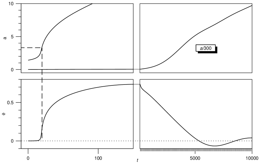
Figure 2: Example for a solution of $a(t)$ and $\phi(t)$ showing early loop inflation and later slow-roll inflation driven by a scalar which is pushed up its potential by loop effects. The left hand side is stretched in time so as to show all details. An idea of the duration of different phases can be obtained from Fig. 3.

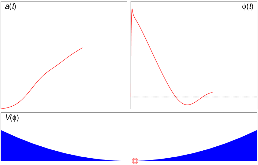
Figure 3: Still of a Movie showing the initial push of a scalar $\phi$ up its potential and the ensuing slow-roll phase together with the corresponding inflationary phase of $a$. The movie is available from the online version [91] of this article at http://relativity.livingreviews.org/Articles/lrr-2005-11/.

In general, we need to know the matter behavior to know $w$ and $w_{\mathrm{eff}}$. But we can get generic qualitative information by treating $p_{\phi}$ and $V(\phi)$ as unknowns determined by $w$ and $w_{\mathrm{eff}}$. In the generic case, there is no unique solution for $p_{\phi}^{2}$ and $V(\phi)$ since, after all, $p_{\phi}$ and $\phi$ change with $t$. They are now subject to two linear equations in terms of $w$ and $w_{\mathrm{eff}}$, whose determinant must be zero resulting in

$$w_{\mathrm{eff}}=-1+\frac{|p|^{3/2}(w+1)(d(p)-\frac{2}{3}|p|d^{\prime}(p))}{1-w+(w+1)|p|^{3/2}d(p)}\,.$$

Since for small $p$ the numerator in the fraction approaches zero faster than the second part of the denominator, $w_{\mathrm{eff}}$ approaches minus one at small volume except for the special case $w=1$ which is realized for $V(\phi)=0$. Note that the argument does not apply to the case of vanishing potential since then $p_{\phi}^{2}=\mathrm{const}$ and $V(\phi)=0$ presents a unique solution to the linear equations for $w$ and $w_{\mathrm{eff}}$. In fact, this case leads in general to a much smaller $w_{\mathrm{eff}}=-\frac{2}{3}|p|d(p)^{\prime}/d(p)\approx-1/(1-l)<-1$ [84].

One can also see from the above formula that $w_{\mathrm{eff}}$, though close to minus one, is a little smaller than minus one generically. This is in contrast to single field inflaton models where the equation of state parameter is a little larger than minus one. As we will discuss in Sec. 4.3.5, this opens the door to characteristic signatures distinguishing different models.

Again, also the matter behavior changes, now with classical friction being replaced by antifriction [85]. Matter fields thus move away from their minima and become excited even if they start close to a minimum (Fig. 2). Since this does not only apply to the homogeneous mode, it can provide a mechanism of structure formation as discussed in Sec. 4.3.5. But also in combination with chaotic inflation as the mechanism to generate structure does the modified matter behavior lead to improvements: if we now view the scalar $\phi$ as an inflaton field, it will be driven to large values in order to start a second phase of slow-roll inflation which is long enough. This is satisfied for a large range of the ambiguity parameters $j$ and $l$ [92] and can even leave signatures [93] in the cosmic microwave spectrum [94]: The earliest moments when the inflaton starts to roll down its potential are not slow roll, as can also be seen in Figs. 2 and 3 where the initial decrease is steeper. Provided the resulting structure can be seen today, i.e. there are not too many e-foldings from the second phase, this can lead to visible effects such as a suppression of power. Whether or not those effects are to be expected, i.e. which magnitude of the inflaton is generically reached by the mechanism generating initial conditions, is currently being investigated at the basic level of loop quantum cosmology [95]. They should be regarded as first suggestions, indicating the potential of quantum cosmological phenomenology, which have to be substantiated by detailed calculations including inhomogeneities or at least anisotropic geometries. In particular the suppression of power can be obtained by a multitude of other mechanisms.

Model building:

It is already clear that there are different inflationary scenarios using effects from loop cosmology. A scenario without inflaton is more attractive since it requires less choices and provides a fundamental explanation of inflation directly from quantum gravity. However, it is also more difficult to analyze structure formation in this context while there are already well-developed techniques in slow role scenarios.

In these cases where one couples loop cosmology to an inflaton model one still requires the same conditions for the potential, but generically gets the required large initial values for the scalar by antifriction. On the other hand, finer details of the results now depend on the ambiguity parameters which describe aspects of the quantization which also arise in the full theory.

It is also possible to combine collapsing and expanding phases in cyclic or oscillatory models [96]. One then has a history of many cycles separated by bounces, whose duration depends on details of the model such as the potential. There can then be many brief cycles until eventually, if the potential is right, one obtains an inflationary phase if the scalar has grown high enough. In this way, one can develop ideas for the pre-history of our universe before the big bang. There are also possibilities to use a bounce to describe the structure in the universe. So far, this has only been described in effective models [97] using brane scenarios [98] where the classical singularity has been assumed to be absent by yet to be determined quantum effects. As it turns out, the explicit mechanism removing singularities in loop cosmology is not compatible with the assumptions made in those effective pictures. In particular, the scalar was supposed to turn around during the bounce which is impossible in loop scenarios unless it encounters a range of positive potential during its evolution [86]. Then, however, generically an inflationary phase commences as in [96] which is then the relevant regime for structure formation. This shows how model building in loop cosmology can distinguish scenarios which are more likely to occur from quantum gravity effects.

Cyclic models can be argued to shift the initial moment of a universe in the infinite past, but they do not explain how the universe started. An attempt to explain this is the emergent universe model [99, 100] where one starts close to a static solution. This is difficult to achieve classically, however, since the available fixed points of the equations of motion are not stable and thus a universe departs too rapidly. Loop cosmology, on the other hand, implies an additional fixed point of the effective equations which is stable and allows to start the universe in an initial phase of oscillations before an inflationary phase is entered [101, 102]. This presents a natural realization of the scenario where the initial scale factor at the fixed point is automatically small so as to start the universe close to the Planck phase.

Stability:

Cosmological equations displaying super-inflation or antifriction are often unstable in the sense that matter can propagate faster than light. This has been voiced as a potential danger for loop cosmology, too [103, 104]. An analysis requires inhomogeneous techniques at least at an effective level, such as those described in Sec. 4.3.2. It has been shown that loop cosmology is free of this problem because the modified behavior for the homogeneous mode of the metric and matter is not relevant for matter propagation [105]. The whole cosmological picture which follows from the effective equations is thus consistent.

4.2 Anisotropies

Anisotropic models provide a first generalization of isotropic ones to more realistic situations. They thus can be used to study the robustness of effects analyzed in isotropic situations and, at the same time, provide a large class of interesting applications. An analysis in particular of the singularity issue is important since the classical approach to a singularity can be very different from the isotropic one. On the other hand, the anisotropic approach is deemed to be characteristic even for general inhomogeneous singularities if the BKL scenario [106] is correct.

4.2.1 Metric variables

A general homogeneous but anisotropic metric is of the form

$$\mathrm{d}s^{2}=-N(t)^{2}\mathrm{d}t^{2}+\sum_{I,J=1}^{3}q_{IJ}(t)\omega^{I}\otimes\omega^{J}$$

with left-invariant 1-forms $\omega^{I}$ on space $\Sigma$ which, thanks to homogeneity, can be identified with the simply transitive symmetry group $S$ as a manifold. The left-invariant 1-forms satisfy the Maurer–Cartan relations

$$\mathrm{d}\omega^{I}=-\frac{1}{2}C^{I}_{JK}\omega^{J}\wedge\omega^{K}$$

with the structure constants $C^{I}_{JK}$ of the symmetry group. In a matrix parameterization of the symmetry group, one can derive explicit expressions for $\omega^{I}$ from the Maurer–Cartan form $\omega^{I}T_{I}=\theta_{MC}=g^{-1}\mathrm{d}g$ with generators $T_{I}$ of $S$.

The simplest case of a symmetry group is an Abelian one with $C^{I}_{JK}=0$, corresponding to the Bianchi I model. In this case, $S$ is given by ${\mathbb{R}}^{3}$ or a torus, and left-invariant 1-forms are simply $\omega^{I}=\mathrm{d}x^{I}$ in Cartesian coordinates. Other groups must be restricted to class A models in this context, satisfying $C^{I}_{JI}=0$ since otherwise there is no Hamiltonian formulation. The structure constants can then be parameterized as $C^{I}_{JK}=\epsilon^{I}_{JK}n^{(I)}$.

A common simplification is to assume the metric to be diagonal at all times, which corresponds to a reduction technically similar to a symmetry reduction. This amounts to $q_{IJ}=a_{(I)}^{2}\delta_{IJ}$ as well as $K_{IJ}=K_{(I)}\delta_{IJ}$ for the extrinsic curvature with $K_{I}=\dot{a}_{I}$. Depending on the structure constants, there is also non-zero intrinsic curvature quantified by the spin connection components

$$\Gamma_{I}=\frac{1}{2}\left(\frac{a_{J}}{a_{K}}n^{J}+\frac{a_{K}}{a_{J}}n^{K}-\frac{a_{I}^{2}}{a_{J}a_{K}}n^{I}\right)\quad\mbox{for}\quad\epsilon_{IJK}=1\,.$$ (33)

This influences the evolution as follows from the Hamiltonian constraint

$$-\frac{1}{8\pi G}\left(a_{1}\dot{a}_{2}\dot{a}_{3}+a_{2}\dot{a}_{1}\dot{a}_{2}+a_{3}\dot{a}_{1}\dot{a}_{2}-(\Gamma_{2}\Gamma_{3}-n^{1}\Gamma_{1})a_{1}-(\Gamma_{1}\Gamma_{3}-n^{2}\Gamma_{2})a_{2}\right.$$

$$-\left.(\Gamma_{1}\Gamma_{2}-n^{3}\Gamma_{3})a_{3}\right)+H_{\mathrm{matter}}(a_{I})=0\,.$$ (34)

In the vacuum Bianchi I case the resulting equations are easy to solve by $a_{I}\propto t^{\alpha_{I}}$ with $\sum_{I}\alpha_{I}=\sum_{I}\alpha_{I}^{2}=1$ [107]. The volume $a_{1}a_{2}a_{3}\propto t$ vanishes for $t=0$ where the classical singularity appears. Since one of the exponents $\alpha_{I}$ must be negative, however, only two of the $a_{I}$ vanish at the classical singularity while the third one diverges. This already demonstrates how different the behavior can be from the isotropic one and that anisotropic models provide a crucial test of any mechanism for singularity resolution.

4.2.2 Connection variables

A densitized triad corresponding to a diagonal homogeneous metric has real components $p^{I}$ with $|p^{I}|=a_{J}a_{K}$ if $\epsilon_{IJK}=1$ [108]. Connection components are $c_{I}=\Gamma_{I}+\gamma K_{I}=\Gamma_{I}+\gamma\dot{a}_{I}$ and are conjugate to the $p_{I}$, $\{c_{I},p^{J}\}=8\pi\gamma G\delta_{I}^{J}$. In terms of triad variables we now have spin connection components

$$\Gamma_{I}=\frac{1}{2}\left(\frac{p^{K}}{p^{J}}n^{J}+\frac{p^{J}}{p^{K}}n^{K}-\frac{p^{J}p^{K}}{(p^{I})^{2}}n^{I}\right)$$ (35)

and the Hamiltonian constraint (in the absence of matter)

$$H = \frac{1}{8\pi G}\left\{\left[(c_{2}\Gamma_{3}+c_{3}\Gamma_{2}-\Gamma_{2}\Gamma_{3})(1+\gamma^{-2})-n^{1}c_{1}-\gamma^{-2}c_{2}c_{3}\right]\sqrt{\left|\frac{p^{2}p^{3}}{p^{1}}\right|}\right.$$ (36)

$$+\left[(c_{1}\Gamma_{3}+c_{3}\Gamma_{1}-\Gamma_{1}\Gamma_{3})(1+\gamma^{-2})-n^{2}c_{2}-\gamma^{-2}c_{1}c_{3}\right]\sqrt{\left|\frac{p^{1}p^{3}}{p^{2}}\right|}$$

$$\left.+\left[(c_{1}\Gamma_{2}+c_{2}\Gamma_{1}-\Gamma_{1}\Gamma_{2})(1+\gamma^{-2})-n^{3}c_{3}-\gamma^{-2}c_{1}c_{2}\right]\sqrt{\left|\frac{p^{1}p^{2}}{p^{3}}\right|}\right\}\,.$$

Unlike in isotropic models, we now have inverse powers of $p^{I}$ even in the vacuum case through the spin connection, unless we are in the Bianchi I model. This is a consequence of the fact that not just extrinsic curvature, which in the isotropic case is related to the matter Hamiltonian through the Friedmann equation, leads to divergences but also intrinsic curvature. These divergences are cut off by quantum geometry effects as before such that also the dynamical behavior changes. This can again be dealt with by effective equations where inverse powers of triad components are replaced by bounded functions [109]. However, even with those modifications, expressions for curvature are not necessarily bounded unlike in the isotropic case. This comes from the presence of different classical scales, $a_{I}$, such that more complicated expressions as in $\Gamma_{I}$ are possible, while in the isotropic model there is only one scale and curvature can only be an inverse power of $p$ which is then regulated by effective expressions like $d(p)$.

4.2.3 Applications

Isotropization:

Matter fields are not the only contributions to the Hamiltonian in cosmology, but also the effect of anisotropies can be included in this way to an isotropic model. The late time behavior of this contribution can be shown to behave as $a^{-6}$ in the shear energy density [110], which falls off faster than any other matter component. Thus, toward later times the universe becomes more and more isotropic.

In the backward direction, on the other hand, this means that the shear term diverges most strongly which suggests that this term should be most relevant for the singularity issue. Even if matter densities are cut off as discussed before, the presence of bounces would depend on the fate of the anisotropy term. This simple reasoning is not true, however, since the behavior of shear is only effective and uses assumptions about the behavior of matter. It can thus not simply be extrapolated to early times. Anisotropies are independent degrees of freedom which affect the evolution of the scale factor. But only in certain regimes can this contribution be modeled simply by a function of the scale factor alone; in general one has to use the coupled system of equations for the scale factor, anisotropies and possible matter fields.

Bianchi IX:

Modifications to classical behavior are most drastic in the Bianchi IX model with symmetry group $S\cong\mathrm{SU}(2)$ such that $n^{I}=1$. The classical evolution can be described by a 3-dimensional mechanics system with a potential obtained from (34) such that the kinetic term is quadratic in derivatives of $a_{I}$ with respect to a time coordinate $\tau$ defined by $\mathrm{d}t=a_{1}a_{2}a_{3}\mathrm{d}\tau$. This potential

$$W(p^{I}) = (\Gamma_{2}\Gamma_{3}-n^{1}\Gamma_{1})p^{2}p^{3}+(\Gamma_{1}\Gamma_{3}-n^{2}\Gamma_{2})p^{1}p^{3}+(\Gamma_{1}\Gamma_{2}-n^{3}\Gamma_{3})p^{1}p^{2}$$

$$= \frac{1}{4}\left(\left(\frac{p^{2}p^{3}}{p^{1}}\right)^{2}+\left(\frac{p^{1}p^{3}}{p^{2}}\right)^{2}+\left(\frac{p^{1}p^{2}}{p^{3}}\right)^{2}-2(p^{1})^{2}-2(p^{2})^{2}-2(p^{3})^{2}\right)$$

diverges at small $p^{I}$, in particular (in a direction dependent manner) at the classical singularity where all $p^{I}=0$. Fig. 4 illustrates the walls of the potential which with decreasing volume push the universe toward the classical singularity.

Figure 4: Still of a Movie illustrating the Bianchi IX potential (4.2.3) and the movement of its walls, rising toward zero $p^{1}$ and $p^{2}$ and along the diagonal direction, toward the classical singularity with decreasing volume $V=\sqrt{|p^{1}p^{2}p^{3}|}$. The contours are plotted for the function $W(p^{1},p^{2},V^{2}/(p^{1}p^{2}))$. The movie is available from the online version [91] of this article at http://relativity.livingreviews.org/Articles/lrr-2005-11/.

As before in isotropic models, effective equations where the behavior of eigenvalues of the spin connection components is used do not have this divergent potential. Instead, if two $p^{I}$ are held fixed and the third approaches zero, the effective quantum potential is cut off and goes back to zero at small values, which changes the approach to the classical singularity. Yet, the effective potential is unbounded if one $p^{I}$ diverges while another one goes to zero and the situation is qualitatively different from the isotropic case. Since the effective potential corresponds to spatial intrinsic curvature, curvature is not bounded in anisotropic effective models. However, this is a statement only about curvature expressions on minisuperspace, and the more relevant question is what happens to curvature along trajectories obtained by solving equations of motion. This demonstrates that dynamical equations must always be considered to draw conclusions for the singularity issue.

The approach to the classical singularity is best analyzed in Misner variables [111] consisting of the scale factor $\Omega:=-\frac{1}{3}\log V$ and two anisotropy parameters $\beta_{\pm}$ defined such that

$$a_{1}=e^{-\Omega+\beta_{+}+\sqrt{3}\beta_{-}}\quad,\quad a_{2}=e^{-\Omega+\beta_{+}-\sqrt{3}\beta_{-}}\quad,\quad a_{3}=e^{-\Omega-2\beta_{+}}\,.$$

The classical potential then takes the form

$$W(\Omega,\beta_{\pm})=\frac{1}{2}e^{-4\Omega}\left(e^{-8\beta_{+}}-4e^{-2\beta_{+}}\cosh(2\sqrt{3}\beta_{-})+2e^{4\beta_{+}}(\cosh(4\sqrt{3}\beta_{-})-1)\right)$$

which at fixed $\Omega$ has three exponential walls rising from the isotropy point $\beta_{\pm}=0$ and enclosing a triangular region (Fig. 5).

Figure 5: Still of a Movie illustrating the Bianchi IX potential in the anisotropy plane and its exponentially rising walls. Positive values of the potential are drawn logarithmically with solid contour lines and negative values with dashed contour lines. The movie is available from the online version [91] of this article at http://relativity.livingreviews.org/Articles/lrr-2005-11/.

A cross section of a wall can be obtained by taking $\beta_{-}=0$ and $\beta_{+}$ to be negative, in which case the potential becomes $W(\Omega,\beta_{+},0)\approx\frac{1}{2}e^{-4\Omega-8\beta_{+}}$. One thus obtains the picture of a point moving almost freely until it is reflected at a wall. In between reflections, the behavior is approximately given by the Kasner solution described before. This behavior with infinitely many reflections before the classical singularity is reached can be shown to be chaotic [112] which suggests a complicated approach to classical singularities in general.

Figure 6: Approximate effective wall of finite height [113] as a function of $x=-\beta_{+}$, compared to the classical exponential wall (upper dashed curve). Also shown is the exact wall $W(p^{1},p^{1},(V/p^{1})^{2})$ (lower dashed curve), which for $x$ smaller than the peak value coincides well with the approximation up to a small, nearly constant shift.

With the effective modification, however, the potential for fixed $\Omega$ does not diverge and the walls, as shown in Fig. 6, break down already at a small but non-zero volume [113]. As a function of densitized triad components the effective potential is illustrated in Fig. 7, and as a function on the anisotropy plane in Fig. 8. In this scenario, there are only finitely many reflections which does not lead to chaotic behavior but instead results in asymptotic Kasner behavior [114].

Figure 7: Still of a Movie illustrating the effective Bianchi IX potential and the movement and breakdown of its walls. The contours are plotted as in Fig. 4. The movie is available from the online version [91] of this article at http://relativity.livingreviews.org/Articles/lrr-2005-11/.

Figure 8: Still of a Movie illustrating the effective Bianchi IX potential in the anisotropy plane and its walls of finite height which disappear at finite volume. Positive values of the potential are drawn logarithmically with solid contour lines and negative values with dashed contour lines. The movie is available from the online version [91] of this article at http://relativity.livingreviews.org/Articles/lrr-2005-11/.

Comparing Fig. 5 with Fig. 8 shows that in their center they are very close to each other, while strong deviations occur for large anisotropies. This demonstrates that most of the classical evolution, which mostly happens in the inner triangular region, is not strongly modified by the effective potential. Quantum effects are important only when anisotropies become too large, for instance when the system moves deep into one of the three valleys, or the total volume becomes small. In those regimes the quantum evolution will take over and describe the further behavior of the system.

Isotropic curvature suppression:

If we use the potential for time coordinate $t$ rather than $\tau$, it is replaced by $W/(p^{1}p^{2}p^{3})$ which in the isotropic reduction $p^{1}=p^{2}=p^{3}=\frac{1}{4}a^{2}$ gives the curvature term $ka^{-2}$. Although the anisotropic effective curvature potential is not bounded it is, unlike the classical curvature, bounded from above at any fixed volume. Moreover, it is bounded along the isotropy line and decays when $a$ approaches zero. Thus, there is a suppression of the divergence in $ka^{-2}$ when the closed isotropic model is viewed as embedded in a Bianchi IX model. Similarly to matter Hamiltonians, intrinsic curvature then approaches zero at zero scale factor.

This is a further illustration for the special nature of isotropic models compared to anisotropic ones. In the classical reduction, the $p^{I}$ in the anisotropic spin connection cancel such that the spin connection is a constant and no special steps are needed for its quantization. By viewing isotropic models within anisotropic ones, one can consistently realize the model and see a suppression of intrinsic curvature terms. Anisotropic models, on the other hand, do not have, and do not need, complete suppression since curvature functions can still be unbounded.

4.2.4 Implications for inhomogeneities

Even without implementing inhomogeneous models the previous discussion allows some tentative conclusions as to the structure of general singularities. This is based on the BKL picture [106] whose basic idea is to study Einstein’s field equations close to a singularity. One can then argue that spatial derivatives become subdominant compared to time-like derivatives such that the approach should locally be described by homogeneous models, in particular the Bianchi IX model since it has the most freedom in its general solution.

Since spatial derivatives are present, though, they lead to small corrections and couple the geometries in different spatial points. One can visualize this by starting with an initial slice which is approximated by a collection of homogeneous patches. For some time, each patch evolves independently of the others, but this is not precisely true since coupling effects have been ignored. Moreover, each patch geometry evolves in a chaotic manner which means that two initially nearby geometries depart rapidly from each other. The approximation can thus be maintained only if the patches are subdivided during the evolution which goes on without limits in the approach to the singularity. There is thus more and more inhomogeneous structure being generated on arbitrarily small scales which leads to a complicated picture of a general singularity.

This picture can be taken over to the effective behavior of the Bianchi IX model. Here, the patches do not evolve chaotically even though at larger volume they follow the classical behavior. The subdivision thus has to be done also for the initial effective evolution. At some point, however, when reflections on the potential walls stop, the evolution simplifies and subdivisions are no longer necessary. There is thus a lower bound to the scale of structure whose precise value depends on the initial geometries. Nevertheless, from the scale at which the potential walls break down one can show that structure formation stops at the latest when the discreteness scale of quantum geometry is reached [113]. This can be seen as a consistency test of the theory since structure below the discreteness could not be supported by quantum geometry.

We have thus a glimpse on the inhomogeneous situation with a complicated but consistent approach to a general classical singularity. The methods involved, however, are not very robust since the BKL scenario, which even classically is still at the level of a conjecture for the general case [112, 115], would need to be available as an approximation to quantum geometry. For more reliable results the methods need to be refined to take into account inhomogeneities properly.

4.3 Inhomogeneities

Allowing for inhomogeneities inevitably means to take a big step from finitely many degrees of freedom to infinitely many ones. There is no straightforward way to cut down the number of degrees of freedom to finitely many ones while being more general than in the homogeneous context. One possibility would be to introduce a small-scale cut-off such that only finitely many wave modes arise (e.g. through a lattice as is indeed done in some coherent state constructions [116]). This is in fact expected to happen in a discrete framework such as quantum geometry, but would at this stage of defining a model simply be introduced by hand.

4.3.1 Available approximations

For the analysis of inhomogeneous situations there are several different approximation schemes:

• Use only isotropic quantum geometry and in particular its effective description, but couple to inhomogeneous matter fields. Problems in this approach are that back-reaction effects are ignored (which is also the case in most classical treatments) and that there is no direct way how to check modifications used in particular for gradient terms of the matter Hamiltonian. So far, this approach has led to a few indications of possible effects.

• Start with the full constraint operator, write it as the homogeneous one plus correction terms from inhomogeneities, and derive effective classical equations. This approach is more ambitious since contact to the full theory is realized. So far, there are not many results since a suitable perturbation scheme has to be developed.

• There are inhomogeneous symmetric models, such as the spherically symmetric one or Einstein–Rosen waves, which have infinitely many kinematical degrees of freedom but can be treated explicitly. Also here, contact to the full theory is present through the symmetry reduction procedure of Sec. 6. This procedure itself can be tested by studying those models between homogeneous ones and the full theory, but results can also be used for physical applications involving inhomogeneities. Many issues which are of importance in the full theory, such as the anomaly problem, also arise here and can thus be studied more explicitly.

4.3.2 Inhomogeneous matter with isotropic quantum geometry

Inhomogeneous matter fields cannot be introduced directly to isotropic quantum geometry since after the symmetry reduction there is no space manifold left for the fields to live on. There are then two different routes to proceed: One can simply take the classical field Hamiltonian and introduce effective modifications modeled on what happens to the isotropic Hamiltonian, or perform a mode decomposition of the matter fields and just work with the space-independent amplitudes. The latter is possible since the homogeneous geometry provides a background for the mode decomposition.

The basic question, for the example of a scalar field, then is how the metric coefficient $E^{a}_{i}E^{b}_{i}/\sqrt{\left|\det E\right|}$ in the gradient term of (12) would be replaced effectively. For the other terms, one can simply use the isotropic modification which is taken directly from the quantization. For the gradient term, however, one does not have a quantum expression in this context and a modification can only be guessed. The problem arises since the inhomogeneous term involves inverse powers of $E$, while in the isotropic context the coefficient just reduces to $\sqrt{|p|}$ which would not be modified at all. There is thus no obvious and unique way to find a suitable replacement.

A possible route would be to read off the modification from the full quantum Hamiltonian, or at least from an inhomogeneous model, which requires a better knowledge of the reduction procedure. Alternatively, one can take a more phenomenological point of view and study the effects of possible replacements. If the robustness of these effects to changes in the replacements is known, one can get a good picture of possible implications. So far, only initial steps have been taken and there is no complete program in this direction.

Another approximation of the inhomogeneous situation has been developed in [117] by patching isotropic quantum geometries together to support an inhomogeneous matter field. This can be used to study modified dispersion relations to the extent that the result agrees with preliminary calculations performed in the full theory [118, 119, 120, 121, 122] even at a quantitative level. There is thus further evidence that symmetric models and their approximations provide reliable insights into the full theory.

4.3.3 Perturbations

With a symmetric background, a mode decomposition is not only possible for matter fields but also for geometry. The homogeneous modes can then be quantized as before, while higher modes are coupled as perturbations implementing inhomogeneities [123]. As with matter Hamiltonians before, one can then also deal with the gravitational part of the Hamiltonian constraint. In particular, there are terms with inverse powers of the homogeneous fields which receive modifications upon quantization. As with gradient terms in matter Hamiltonians, there are several options for those modifications which can only be restricted by relating them to the full Hamiltonian. This would require introducing the mode decomposition, analogously to symmetry conditions, at the quantum level and writing the full constraint operator as the homogeneous one plus correction terms.

An additional complication compared to matter fields is that one is now dealing with infinitely many coupled constraint equations since the lapse function $N(x)$ is inhomogeneous, too. This function can itself be decomposed into modes $\sum_{n}N_{n}Y_{n}(x)$, with harmonics $Y_{n}(x)$ according to the symmetry, and each amplitude $N_{n}$ is varied independently giving rise to a separate constraint. The main constraint arises from the homogeneous mode, which describes how inhomogeneities affect the evolution of the homogeneous scale factors.

4.3.4 Inhomogeneous models

The full theory is complicated at several different levels of both conceptual and technical nature. For instance, one has to deal with infinitely many degrees of freedom, most operators have complicated actions, and interpreting solutions to all constraints in a geometrical manner can be difficult. Most of these complications are avoided in homogeneous models, in particular when effective classical equations are employed. These equations use approximations of expectation values of quantum geometrical operators which need to be known rather explicitly. The question then arises whether one can still work at this level while relaxing the symmetry conditions and bringing in more complications of the full theory.

Explicit calculations at a level similar to homogeneous models, at least for matrix elements of individual operators, are possible in inhomogeneous models, too. In particular the spherically symmetric model and cylindrically symmetric Einstein–Rosen waves are of this class, where the symmetry or other conditions are strong enough to result in a simple volume operator. In the spherically symmetric model this simplification comes from the remaining isotropy subgroup isomorphic to U(1) in generic points, while the Einstein–Rosen model is simplified by polarization conditions which play a role analogous to the diagonalization of homogeneous models. With these models one obtains access to applications for black holes and gravitational waves, but also to inhomogeneities in cosmology.

In spherical coordinates $x$, $\vartheta$, $\varphi$ a spherically symmetric spatial metric takes the form

$$\mathrm{d}s^{2}=q_{xx}(x,t)\mathrm{d}x^{2}+q_{\varphi\varphi}(x,t)\mathrm{d}\Omega^{2}$$

with $\mathrm{d}\Omega^{2}=\mathrm{d}\vartheta^{2}+\sin^{2}\vartheta\mathrm{d}\varphi^{2}$. This is related to densitized triad components by [124, 125]

$$|E^{x}|=q_{\varphi\varphi}\quad,\quad(E^{\varphi})^{2}=q_{xx}q_{\varphi\varphi}$$

which are conjugate to the other basic variables given by the Ashtekar connection component $A_{x}$ and the extrinsic curvature component $K_{\varphi}$:

$$\{A_{x}(x),E^{x}(y)\}=8\pi G\gamma\delta(x,y)\quad,\quad\{\gamma K_{\varphi}(x),E^{\varphi}(y)\}=16\pi G\gamma\delta(x,y)\,.$$

Note that we use the Ashtekar connection for the inhomogeneous direction $x$ but extrinsic curvature for the homogeneous direction along symmetry orbits [126]. Connection and extrinsic curvature components for the $\varphi$-direction are related by $A_{\varphi}^{2}=\Gamma_{\varphi}^{2}+\gamma^{2}K_{\varphi}^{2}$ with the spin connection component

$$\Gamma_{\varphi}=-\frac{E^{x\prime}}{2E^{\varphi}}\,.$$ (38)

Unlike in the full theory or homogeneous models, $A_{\varphi}$ is not conjugate to a triad component but to [127]

$$P^{\varphi}=\sqrt{4(E^{\varphi})^{2}-A_{\varphi}^{-2}(P^{\beta})^{2}}$$

with the momentum $P^{\beta}$ conjugate to a U(1)-gauge angle $\beta$. This is a rather complicated function of both triad and connection variables such that the volume $V=4\pi\int\sqrt{|E^{x}|}E^{\varphi}\mathrm{d}x$ would have a rather complicated quantization. It would still be possible to compute the full volume spectrum, but with the disadvantage that volume eigenstates would not be given by triad eigenstates such that computations of many operators would be complicated [128]. This can be avoided by using extrinsic curvature which is conjugate to the triad component [126]. Moreover, this is also in accordance with a general scheme to construct Hamiltonian constraint operators for the full theory as well as symmetric models [65, 129, 130].

The constraint operator in spherical symmetry is given by

$$H[N]=-(2G)^{-1}\int_{B}\mathrm{d}xN(x)|E^{x}|^{-1/2}\left((K_{\varphi}^{2}E^{\varphi}+2K_{\varphi}K_{x}E^{x})+(1-\Gamma_{\varphi}^{2})E^{\varphi}+2\Gamma_{\varphi}^{\prime}E^{x}\right)$$ (39)

accompanied by the diffeomorphism constraint

$$D[N^{x}]=(2G)^{-1}\int_{B}N^{x}(x)(2E^{\varphi}K_{\varphi}^{\prime}-K_{x}E^{x\prime})\,.$$ (40)

We have expressed this in terms of $K_{x}$ for simplicity, keeping in mind that as the basic variable for quantization we will later use the connection component $A_{x}$.

Since the Hamiltonian constraint contains the spin connection component $\Gamma_{\varphi}$ given by (38), which contains inverse powers of densitized triad components, one can expect effective classical equations with modifications similar to the Bianchi IX model. However, the situation is now much more complicated since we have a system constrained by many constraints with a non-Abelian algebra. Simply replacing the inverse of $E^{\varphi}$ by a bounded function as before will change the constraint algebra and thus most likely lead to anomalies. It is currently open if a more refined replacement can be done where not only the spin connection but also the extrinsic curvature terms are modified. This issue has the potential to shed light on many questions related to the anomaly issue. It is one of the cases where models between homogeneous ones, where the anomaly problem trivializes, and the full theory are most helpful.

4.3.5 Results

There are some results obtained for inhomogeneous systems. We have already discussed glimpses from the BKL picture, which used loop results only for anisotropic models. Methods described in this section have led to some preliminary insights into possible cosmological scenarios.

Matter gradient terms and small-$a$ effects:

When an inhomogeneous matter Hamiltonian is available it is possible to study its implications on the cosmic microwave background with standard techniques. With modifications of densities there are then different regimes since the part of the inflationary era responsible for the formation of currently visible structure can be in the small-$a$ or large-$a$ region of the effective density.

The small-$a$ regime below the peak of effective densities has more dramatic effects since inflation can here be provided by quantum geometry effects alone and the matter behavior changes to be anti-frictional [84, 85]. Mode evolution in this regime has been investigated for a particular choice of gradient term and using a power-law approximation for the effective density at small $a$, with the result that there are characteristic signatures [131]. As in standard inflation models the spectrum is nearly scale invariant, but its spectral index is slightly larger than one (blue tilt) as compared to slightly smaller than one (red tilt) for single-field inflaton models. Since small scale factors at early stages of inflation generate structure which today appears on the largest scales, this implies that low multipoles of the power spectrum should have a blue tilt. The running of the spectral index in this regime can also be computed but depends only weakly on ambiguity parameters.

The main parameter then is the duration of loop inflation. In the simplest scenario one can assume only one inflationary phase which would require huge values for the ambiguity parameter $j$. This is unnatural and would imply that the spectrum is blue on almost all scales which is in conflict with present observations. Thus, not only conceptual arguments but also cosmological observations point to smaller values for $j$, which is quite remarkable.

In order to have sufficient inflation to make the universe big enough one then needs additional stages provided by the behavior of matter fields. One still does not need an inflaton since now the details of the expansion after the structure generating phase are less important. Any matter field being driven away from its potential minimum during loop inflation and rolling down its potential thereafter suffices. Depending on the complexity of the model there can be several such phases.

Matter gradient terms and large-$a$ effects:

At larger scale factors above the peak of effective densities there are only perturbative corrections from loop effects. This has been investigated with the aim of finding trans-Planckian corrections to the microwave background, also here with a particular gradient term. In this model, cancellations have been observed which imply that corrections appear only at higher orders of the perturbation series and are too weak to be observable [132].

A common problem of both analyses is that the robustness of the observed effects has not yet been studied. This is in particular a pressing problem since one modification of the gradient term has been chosen without further motivation. Moreover, the modifications in both examples were different. Without a more direct derivation of the modifications from inhomogeneous models or the full theory one can only rely on a robustness analysis to show that the effects can be trusted. In particular the cancellation in the second example must be shown to be realized for a larger class of modifications.

Non-inflationary structure formation:

Given a modification of the gradient term one obtains effective equations for the matter field which for a scalar results in a modified Klein–Gordon equation. After a mode decomposition one can then easily see that all the modes behave differently at small scales with the classical friction replaced by anti-friction as in Sec. 4.1.5. Thus, not only the average value of the field is driven away from its potential minimum but also higher modes are being excited. The coupled dynamics of all the modes thus provides a scenario for structure formation which does not rely on inflation but on the anti-friction effect of loop cosmology.

Even though all modes experience this effect, they do not all see it in the same way. The gradient term implies an additive contribution to the potential proportional to $k^{2}$ for a mode of wave number $k$, which also depends on the metric in a way determined by the gradient term modification. For larger scales, the additional term is not essential and their amplitudes will be pushed to similar magnitudes, suggesting scale invariance for them. The potential relevant for higher modes, however, becomes steeper and steeper such that they are less excited by anti-friction and retain a small initial amplitude. In this way, the structure formation scenario provides a dynamical mechanism for a small-scale cut-off, possibly realizing older expectations [133, 134].

Stability:

As already noted, inhomogeneous matter Hamiltonians can be used to study the stability of cosmological equations in the sense that matter does not propagate faster than light. The modified behavior of homogeneous modes has led to the suspicion that loop cosmology is not stable [103, 104] since other cosmological models displaying super-inflation have this problem. A detailed analysis of the loop equations, however, shows that the equations as they arise from modifications are automatically stable. While the homogeneous modes display super-inflationary and anti-frictional behavior, they are not relevant for matter propagation. Modes relevant for propagation, on the other hand, are modified differently in such a manner that the total behavior is stable [105]. Most importantly, this is an example where an inhomogeneous matter Hamiltonian with its modifications must be used and the qualitative result of stability can be shown to be robust under possible changes of the effective modification. This shows that reliable conclusions can be drawn for important issues without a precise definition of the effective inhomogeneous behavior.

4.4 Summary

Loop cosmology is an effective description of quantum effects in cosmology, obtained in a framework of a background independent and non-perturbative quantization. There is mainly one change compared to classical equations coming from modified densities in matter Hamiltonians or also anisotropy potentials. These modifications are non-perturbative as they contain inverse powers of the Planck length and thus the gravitational constant, but also perturbative corrections arise from curvature terms, which are now being studied.

The non-perturbative modification alone is responsible for a surprising variety of phenomena which all improve the behavior in classical cosmology. Nevertheless, the modification had not been motivated by phenomenology but derived through the background independent quantization. Details of its derivation in cosmological models and its technical origin will now be reviewed in Sec. 5, before we come to a discussion of the link to the full theory in Sec. 6.

5 Loop quantization of symmetric models

Analogies prove nothing, but they can make one feel more at home.

Sigmund Freud

Introductory Lectures on Psychoanalysis

In full loop quantum gravity, the quantum representation is crucial for the foundation of the theory. The guiding theme there is background independence which requires one to smear the basic fields in a particular manner to holonomies and fluxes. In this section we will see what implications this has for composite operators and the physical effects they entail. We will base this analysis on symmetric models in order to be able to perform explicit calculations.

Symmetries are usually introduced in order to simplify calculations or make them possible in the first place. However, symmetries can sometimes also lead to complications in conceptual questions if the additional structure they provide is not fully taken into account. In the present context, it is important to realize that the action of a symmetry group on a space manifold provides a partial background such that the situation is always slightly different from the full theory. If the symmetry is strong, such as in homogeneous models, other representations such as the Wheeler–DeWitt representation can be possible even though the fact that a background has been used may not be obvious. While large scale physics is not very sensitive to the representation used, it becomes very important on the smallest scales which we have to take into account when the singularity issue is considered.

Instead of looking only at one symmetric model where one may have different possibilities to choose the basic representation, one should thus keep the full view on different models as well as the full theory. In fact, in loop quantum gravity it is possible to relate models and the full theory such that symmetric states and basic operators, and thus the representation, can be derived from the unique background independent representation of the full theory. We will describe this in detail in Sec. 6, after having discussed the construction of quantum models in the present section. Without making use of the relation to the full theory, one can construct models by analogy. This means that quantization steps are modeled on those which are known to be crucial in the full theory, which starts with the basic representation and continues to the Hamiltonian constraint operator. One can then disentangle places where additional input as compared to the full theory is needed and which implications it has.

5.1 Symmetries and backgrounds

It is impossible to introduce symmetries in a completely background independent manner. The mathematical action of a symmetry group is defined by a mapping between abstract points which do not exist in a diffeomorphism invariant setting (if one, for instance, considers only equivalence classes up to arbitrary diffeomorphisms).

More precisely, while the full theory has as background only a differentiable or analytic manifold $\Sigma$, a symmetric model has as background a symmetric manifold $(\Sigma,S)$ consisting of a differentiable or analytic manifold $\Sigma$ together with an action of a symmetry group $S\colon\Sigma\to\Sigma$. How strong the additional structure is depends on the symmetry used. The strongest symmetry in gravitational models is realized with spatial isotropy which implies a unique spatial metric up to a scale factor. The background is thus equivalent to a conformal space.

All constructions in a given model must take its symmetry into account since otherwise its particular dynamics, for instance, could not be captured. The structure of models thus depends on the different types of background realized for different symmetry groups. This can not only lead to simplifications but also to conceptual differences, and it is always instructive to keep the complete view on different models as well as the full theory. Since the loop formalism is general enough to encompass all relevant models, there are many ways to compare and relate different systems. It is thus possible to observe characteristic features of (metric) background independence even in cases where more structure is available.

5.2 Isotropy

Isotropic models are described purely in terms of the scale factor $a(t)$ such that there is only a single kinematical degree of freedom. In connection variables, this is parameterized by the triad component $p$ conjugate to the connection component $c$.

5.2.1 Representation

If we restrict ourselves to invariant connections of a given form, it suffices to probe them with only special holonomies. For an isotropic connection $A_{a}^{i}=\tilde{c}\Lambda^{i}_{I}\omega_{a}^{I}$ (see App. B.2) we can choose holonomies along one integral curve of a symmetry generator $X_{I}$. They are of the form

$$h_{I}=\exp\int A_{a}^{i}X_{I}^{a}\tau_{i}=\cos{\textstyle\frac{1}{2}}\mu c+2\Lambda_{I}^{i}\tau_{i}\sin{\textstyle\frac{1}{2}}\mu c$$ (41)

where $\mu$ depends on the parameter length of the curve and can be any real number (thanks to homogeneity, path ordering is not necessary). Since knowing the values $\cos\frac{1}{2}\mu$ and $\sin\frac{1}{2}\mu c$ for all $\mu$ uniquely determines the value of $c$, which is the only gauge invariant information contained in the connection, these holonomies describe the configuration space of connections completely.

This illustrates how symmetric configurations allow one to simplify the constructions behind the full theory. But it also shows which effects the presence of a partial background can have on the formalism [73]. In the present case the background enters through the left-invariant 1-forms $\omega^{I}$ defined on the spatial manifold whose influence is contained in the parameter $\mu$. All information about the edge used to compute the holonomy is contained in this single parameter which leads to degeneracies compared to the full theory. Most importantly, one cannot distinguish between the parameter length and the spin label of an edge: Taking a power of the holonomy in a non-fundamental representation simply rescales $\mu$, which could just as well come from a longer parameter length. That this is related to the presence of a background can be seen by looking at the roles of edges and spin labels in the full theory. There, both concepts are independent and appear very differently. While the embedding of an edge, including its parameter length, is removed by diffeomorphism invariance, the spin label remains well-defined and is important for ambiguities of operators. In the model, however, the full diffeomorphism invariance is not available such that some information about edges remains in the theory and merges with the spin label. Issues like that have to be taken into account when constructing operators in a model and comparing with the full theory.

Compactification:

The functions appearing in holonomies for isotropic connections define the algebra of functions on the classical configuration space which, together with fluxes, is to be represented on a Hilbert space. This algebra does not contain arbitrary continuous functions of $c$ but only almost periodic ones of the form [73]

$$f(c)=\sum_{\mu}f_{\mu}\exp(i\mu c/2)$$ (42)

where the sum is over a countable subset of ${\mathbb{R}}$. This is analogous to the full situation, reviewed in Sec. 3.4, where matrix elements of holonomies define a special algebra of continuous functions of connections. As in this case, the algebra can be represented as the set of all continuous functions on a compact space, called its spectrum. This compactification can be imagined as being obtained from enlarging the classical configuration space ${\mathbb{R}}$ by adding points, and thus more continuity conditions, until only functions of the given algebra survive as continuous ones. A well-known example is the one point compactification which is the spectrum of the algebra of continuous functions $f$ for which $\lim_{x\to-\infty}f(x)=\lim_{x\to\infty}f(x)$ exists. In this case, one just needs to add a single point at infinity.

In the present case, the procedure is more complicated and leads to the Bohr compactification $\bar{\mathbb{R}}_{\mathrm{Bohr}}$ which contains ${\mathbb{R}}$ densely. It is very different from the one point compactification, as can be seen from the fact that the only function which is continuous on both spaces is the zero function. In contrast to the one point compactification, the Bohr compactification is an Abelian group, just like ${\mathbb{R}}$ itself. Moreover, there is a one-to-one correspondence between irreducible representations of ${\mathbb{R}}$ and irreducible representations of $\bar{\mathbb{R}}_{\mathrm{Bohr}}$, which can also be used as the definition of the Bohr compactification. Representations of $\bar{\mathbb{R}}_{\mathrm{Bohr}}$ are thus labeled by real numbers and given by $\rho_{\mu}\colon\bar{\mathbb{R}}_{\mathrm{Bohr}}\to{\mathbb{C}},c\mapsto e^{i\mu c}$. As with any compact group, there is a unique normalized Haar measure $\mathrm{d}\mu(c)$ given by

$$\int_{\bar{\mathbb{R}}_{\mathrm{Bohr}}}f(c)\mathrm{d}\mu(c)=\lim_{T\to\infty}\frac{1}{2T}\int_{-T}^{T}f(c)\mathrm{d}c$$ (43)

where on the right hand side the Lebesgue measure on ${\mathbb{R}}$ is used.

The Haar measure defines the inner product for the Hilbert space $L^{2}(\bar{\mathbb{R}}_{\mathrm{Bohr}},\mathrm{d}\mu(c))$ of square integrable functions on the quantum configuration space. As one can easily check, exponentials of the form $\langle c|\mu\rangle=e^{i\mu c/2}$ are normalized and orthogonal to each other for different $\mu$,

$$\langle\mu_{1}|\mu_{2}\rangle=\delta_{\mu_{1},\mu_{2}}$$ (44)

which demonstrates that the Hilbert space is not separable.

Similarly to holonomies, one needs to consider fluxes only for special surfaces, and all information is contained in the single number $p$. Since it is conjugate to $c$, it is quantized to a derivative operator

$$\hat{p}=-\frac{1}{3}i\gamma\ell_{\mathrm{P}}^{2}\frac{\mathrm{d}}{\mathrm{d}c}$$ (45)

whose action

$$\hat{p}|\mu\rangle=\frac{1}{6}\gamma\ell_{\mathrm{P}}^{2}\mu|\mu\rangle=:p_{\mu}|\mu\rangle$$ (46)

on basis states $|\mu\rangle$ can easily be determined. In fact, the basis states are eigenstates of the flux operator which demonstrates that the flux spectrum is discrete (all eigenstates are normalizable).

This property is analogous to the full theory with its discrete flux spectra, and similarly it implies discrete quantum geometry. We thus see that the discreteness survives the symmetry reduction in this framework [135]. Similarly, the fact that only holonomies are represented in the full theory but not connection components is realized in the model, too. In fact, we have so far represented only exponentials of $c$, and one can see that these operators are not continuous in the parameter $\mu$. Thus, an operator quantizing $c$ directly does not exist on the Hilbert space. These properties are analogous to the full theory, but very different from the Wheeler–DeWitt quantization. In fact, the resulting representations in isotropic models are inequivalent. While the representation is not of crucial importance when only small energies or large scales are involved [77], it becomes essential at small scales which are in particular realized in cosmology.

5.2.2 Matter Hamiltonian

We now know how the basic quantities $p$ and $c$ are quantized, and can use the operators to construct more complicated ones. Of particular importance, also for cosmology, are matter Hamiltonians where now not only the matter field but also geometry is quantized. For an isotropic geometry and a scalar, this requires us to quantize $|p|^{-3/2}$ for the kinetic term and $|p|^{3/2}$ for the potential term. The latter can be defined readily as $|\hat{p}|^{3/2}$, but for the former we need an inverse power of $p$. Since $\hat{p}$ has a discrete spectrum containing zero, a densely defined inverse does not exist.

At this point, one has to find an alternative route to the quantization of $d(p)=|p|^{-3/2}$, or else one could only conclude that there is no well-defined quantization of matter Hamiltonians as a manifestation of the classical divergence. In the case of loop quantum cosmology it turns out, following a general scheme of the full theory [64], that one can reformulate the classical expression in an equivalent way such that quantization becomes possible. One possibility is to write, similarly to (13)

$$d(p)=\left(\frac{1}{3\pi\gamma G}\sum_{I=1}^{3}\mathrm{tr}\left(\tau_{I}h_{I}\{h_{I}^{-1},\sqrt{V}\}\right)\right)^{6}$$

where we use holonomies of isotropic connections and the volume $V=|p|^{3/2}$. In this expression we can insert holonomies as multiplication operators and the volume operator, and turn the Poisson bracket into a commutator. The result

$$\widehat{d(p)}=\left(8i\gamma^{-1}\ell_{\mathrm{P}}^{-2}(\sin{\textstyle\frac{1}{2}}c\sqrt{\hat{V}}\cos{\textstyle\frac{1}{2}}c-\cos{\textstyle\frac{1}{2}}c\sqrt{\hat{V}}\sin{\textstyle\frac{1}{2}}c)\right)^{6}$$ (47)

is not only a densely defined operator but even bounded, which one can easily read off from the eigenvalues [78]

$$\widehat{d(p)}|\mu\rangle=\left(4\gamma^{-1}\ell_{\mathrm{P}}^{-2}(\sqrt{V_{\mu+1}}-\sqrt{V_{\mu-1}}\,)\right)^{6}|\mu\rangle$$ (48)

with $V_{\mu}=|p_{\mu}|^{3/2}$ and $p_{\mu}$ from (46).

Rewriting a classical expression in such a manner can always be done in many equivalent ways, which in general all lead to different operators. In the case of $|p|^{-3/2}$, we highlight the choice of the representation in which to take the trace (understood as the fundamental representation above) and the power of $|p|$ in the Poisson bracket ($\sqrt{V}=|p|^{3/4}$ above). This freedom can be parameterized by two ambiguity parameters $j\in\frac{1}{2}{\mathbb{N}}$ for the representation and $0<l<1$ for the power such that

$$d(p)=\left(\frac{3}{8\pi\gamma Glj(j+1)(2j+1)}\sum_{I=1}^{3}\mathrm{tr}_{j}(\tau_{I}h_{I}\{h_{I}^{-1},|p|^{l}\})\right)^{3/(2-2l)}\,.$$

Following the same procedure as above, we obtain eigenvalues [79, 13]

$$\widehat{d(p)}^{(\mu)}_{j,l}=\left(\frac{9}{\gamma\ell_{\mathrm{P}}^{2}lj(j+1)(2j+1)}\sum_{k=-j}^{j}k|p_{\mu+2k}|^{l}\right)^{3/(2-2l)}$$

which, for larger $j$, can be approximated by (25), see also Fig. 9. This provides the basis for loop cosmology as described in Sec. 4.

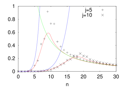
Figure 9: Discrete subset of eigenvalues of $\widehat{d(p)}$ (left) for two choices of $j$ (and $l=\frac{3}{4}$), together with the approximation $d(p)_{j,l}$ from (25) and small-$p$ power laws. The classical divergence at small $p$, where the behavior is strongly modified, is cut off. The right panel shows the dependence of the initial increase on $l$.

Notice that operators for the scale factor, volume or their inverse powers do not refer to observable quantities. It can thus be dangerous, though suggestive, to view their properties as possible bounds on curvature. The importance of operators for inverse volume comes from the fact that this appears in matter Hamiltonians, and thus the Hamiltonian constraint of gravity. Properties of those operators such as their boundedness or unboundedness can then determine the dynamical behavior (see, e.g., [136]).

5.2.3 Hamiltonian constraint

Dynamics is controlled by the Hamiltonian constraint, which classically gives the Friedmann equation. Since the classical expression (28) contains the connection component $c$, we have to use holonomy operators. In the quantum algebra we only have almost periodic functions at our disposal, which does not include polynomials such as $c^{2}$. Quantum expressions can therefore only coincide with the classical one in appropriate limits, which in isotropic cosmology is realized for small extrinsic curvature, i.e. small $c$ in the flat case. We thus need an almost periodic function of $c$ which for small $c$ approaches $c^{2}$. This can easily be found, e.g., the function $\sin^{2}c$. Again, the procedure is not unique since there are many such possibilities, e.g. $\delta^{-2}\sin^{2}\delta c$, and more quantization ambiguities ensue. In contrast to the density $|p|^{-3/2}$, where we also used holonomies in the reformulation, the expressions are not equivalent to each other classically but only in the small curvature regime. As we will discuss shortly, the resulting new terms have the interpretation of higher order corrections to the classical Hamiltonian.

One can restrict the ambiguities to some degree by modeling the expression on that of the full theory. This means that one does not simply replace $c^{2}$ by an almost periodic function, but uses holonomies tracing out closed loops formed by symmetry generators [129, 9]. Moreover, the procedure can be embedded in a general scheme which encompasses different models and the full theory [65, 129, 130], further reducing ambiguities. In particular models with non-zero intrinsic curvature on their symmetry orbits, such as the closed isotropic model, can then be included in the construction. One issue to keep in mind is the fact that “holonomies” are treated differently in models and the full theory. In the latter case, they are ordinary holonomies along edges, which can be shrunk and then approximate connection components. In models, on the other hand, one sometimes uses direct exponentials of connection components without integration. In such a case, connection components are approximated only when they are small; if they are not, the corresponding objects such as the Hamiltonian constraint receive infinitely many correction terms of higher powers in curvature (similarly to effective actions). The difference between both ways of dealing with holonomies can be understood in inhomogeneous models, where they are both realized for different connection components.

In the flat case the construction is easiest, related to the Abelian nature of the symmetry group. One can directly use the exponentials $h_{I}$ in (41), viewed as 3-dimensional holonomies along integral curves, and mimic the full constraint where one follows a loop to get curvature components of the connection $A_{a}^{i}$. Respecting the symmetry, this can be done in the model with a square loop in two independent directions $I$ and $J$. This yields the product $h_{I}h_{J}h_{I}^{-1}h_{J}^{-1}$, which appears in a trace, as in (15), together with a commutator $h_{K}[h_{K}^{-1},\hat{V}]$ using the remaining direction $K$. The latter, following the general scheme of the full theory reviewed in Sec. 3.6, quantizes the contribution $\sqrt{|p|}$ to the constraint, instead of directly using the simpler $\sqrt{|\hat{p}|}$.

Taking the trace one obtains a diagonal operator

$$\sin({\textstyle\frac{1}{2}}\delta c)\hat{V}\cos({\textstyle\frac{1}{2}}\delta c)-\cos({\textstyle\frac{1}{2}}\delta c)\hat{V}\sin({\textstyle\frac{1}{2}}\delta c)$$

in terms of the volume operator, as well as the multiplication operator

$$\sin^{2}({\textstyle\frac{1}{2}}\delta c)\cos^{2}({\textstyle\frac{1}{2}}\delta c)=\sin^{2}(\delta c)\,.$$

In the triad representation where instead of working with functions $\langle c|\psi\rangle=\psi(c)$ one works with the coefficients $\psi_{\mu}$ in an expansion $|\psi\rangle=\sum_{\mu}\psi_{\mu}|\mu\rangle$, this operator is the square of a difference operator. The constraint equation thus takes the form of a difference equation [9, 85, 73]

$$(V_{\mu+5\delta}-V_{\mu+3\delta})e^{ik}\psi_{\mu+4\delta}(\phi)-(2+k^{2}\gamma^{2}\delta^{2})(V_{\mu+\delta}-V_{\mu-\delta})\psi_{\mu}(\phi)$$

$$+(V_{\mu-3\delta}-V_{\mu-5\delta})e^{-ik}\psi_{\mu-4\delta}(\phi)=-\frac{16\pi}{3}G\gamma^{3}\delta^{3}\ell_{\mathrm{P}}^{2}\hat{H}_{\mathrm{matter}}(\mu)\psi_{\mu}(\phi)$$ (49)

for the wave function $\psi_{\mu}$ which can be viewed as an evolution equation in internal time $\mu$. (Note that this equation is not valid for $k=-1$ since the derivation via a Hamiltonian formulation is not available in this case.) Thus, discrete spatial geometry implies a discrete internal time [137]. The equation above results in the most direct way from a non-symmetric constraint operator with gravitational part acting as

$$\hat{H}|\mu\rangle=\frac{3}{16\pi G\gamma^{3}\delta^{3}\ell_{\mathrm{P}}^{2}}(V_{\mu+\delta}-V_{\mu-\delta})(e^{-ik}|\mu+4\delta\rangle-(2+k^{2}\gamma^{2}\delta^{2})|\mu\rangle+e^{ik}|\mu-4\delta\rangle)\,.$$

One can symmetrize this operator and obtain a difference equation with different coefficients, which we do here after multiplying the operator with $\widehat{\mathrm{sgn}p}$ for reasons that will be discussed in the context of singularities in Sec. 5.6.3. The resulting difference equation is

$$(|\Delta_{\delta}V|(\mu+4\delta)+|\Delta_{\delta}V|(\mu))e^{ik}\psi_{\mu+4\delta}(\phi)-2(2+k^{2}\gamma^{2}\delta^{2})|\Delta_{\delta}V|(\mu)\psi_{\mu}(\phi)$$

$$+(|\Delta_{\delta}V|(\mu-4\delta)+|\Delta_{\delta}V|(\mu))e^{-ik}\psi_{\mu-4\delta}(\phi)=-\frac{32\pi}{3}G\gamma^{3}\delta^{3}\ell_{\mathrm{P}}^{2}\hat{H}_{\mathrm{matter}}(\mu)\psi_{\mu}(\phi)$$ (50)

where $|\Delta_{\delta}V|(\mu):=\mathrm{sgn}(\mu)(V_{\mu+\delta}-V_{\mu-\delta})=|V_{\mu+\delta}-V_{\mu-\delta}|$.

Since $\sin c|\mu\rangle=-\frac{1}{2}i(|\mu+2\rangle-|\mu-2\rangle)$, the difference equation is of higher order, even formulated on an uncountable set, and thus has many independent solutions. Most of them, however, oscillate on small scales, i.e. between $\mu$ and $\mu+m\delta$ with small integer $m$. Others oscillate only on larger scales and can be viewed as approximating continuum solutions. The behavior of all the solutions leads to possibilities for selection criteria of different versions of the constraint since there are quantization choices. Most importantly, one chooses the routing of edges to construct the square holonomy, again the spin of a representation to take the trace [68, 138], and factor ordering choices between quantizations of $c^{2}$ and $\sqrt{|p|}$. All these choices also appear in the full theory such that one can draw conclusions for preferred cases there.

When the symmetry group is not Abelian and there is non-zero intrinsic curvature, the construction is more complicated. For non-Abelian symmetry groups integral curves as before do not form a closed loop and one needs a correction term related to intrinsic curvature components [9, 109]. Moreover, the classical regime is not as straightforward to specify since connection components are not necessarily small when there is intrinsic curvature. A general scheme encompassing intrinsic curvature, other symmetric models and the full theory will be discussed in Sec. 5.6.2.

5.2.4 Semiclassical limit and correction terms

When replacing $c^{2}$ by holonomies we have modified the constraint as a function on the classical phase space. This is necessary since otherwise the function cannot be quantized, but is different from the quantization of densities because now the replacements are not equivalent to the original constraint classically. Also the limit $\lim_{\delta\to 0}\delta^{-2}\sin^{2}\delta c$, which would give the classical result, does not exist at the operator level.

This situation is different from the full theory, again related to the presence of a partial background [73]. There, the parameter length of edges used to construct appropriate loops is irrelevant and thus can shrink to zero. In the model, however, changing the edge length with respect to the background does change the operator and the limit does not exist. Intuitively, this can be understood as follows: The full constraint operator (15) is a vertex sum obtained after introducing a discretization of space used to choose loops $\alpha_{IJ}$. This classical regularization sums over all tetrahedra in the discretization, whose number diverges in the limit where the discretization size shrinks to zero. In the quantization, however, almost all these contributions vanish since a tetrahedron must contain a vertex of a state in order to contribute non-trivially. The result is independent of the discretization size once it is fine enough, and the limit can thus be taken trivially.

In a homogeneous model, on the other hand, contributions from different tetrahedra of the triangulation must be identical owing to homogeneity. The coordinate size of tetrahedra drops out of the construction in the full background independent quantization, as emphasized in Sec. 3.6, which is part of the reason for the discretization independence. In a homogeneous configuration the number of contributions thus increases in the limit, but their size does not change. This results in an ill-defined limit as we have already seen within the model itself.

The difference between models and the full theory is thus only a consequence of the symmetry and not of different approaches. This will also become clear later in inhomogeneous models where one obtains a mixture between the two situations. Moreover, in the full theory one has a situation similar to symmetric models if one does not only look at the operator limit when the regularization is removed but also checks the classical limit on semiclassical states. In homogeneous models, the expression in terms of holonomies implies corrections to the classical constraint when curvature becomes larger. This is in analogy to other quantum field theories where effective actions generally have higher curvature terms. In the full theory, those correction terms can be seen when one computes expectation values of the Hamiltonian constraint in semiclassical states peaked at classical configurations for the connection and triad. When this classical configuration becomes small in volume or large in curvature, correction terms to the classical constraint arise. In this case, the semiclassical state provides the background with respect to which these corrections appear. In a homogeneous model, the symmetry already provides a partial background such that correction terms can be noticed already for the constraint operator itself.

WKB approximation:

There are different procedures to make contact between the difference equation and classical constraints. The most straightforward way is to expand the difference operators in a Taylor series, assuming that the wave function is sufficiently smooth. On large scales, this indeed results in the Wheeler–DeWitt equation as a continuum limit in a particular ordering [139]. From then on, one can use the WKB approximation or Wigner functions as usually.

That this is possible may be surprising because as just discussed the continuum limit $\delta\to 0$ does not exist for the constraint operator. And indeed, the limit of the constraint equation, i.e. the operator applied to a wave function, does not exist in general. Even for a wave function the limit $\delta\to 0$ does not exist in general since some solutions are sensitive to the discreteness and do not have a continuum limit at all. When performing the Taylor expansion we already assumed certain properties of the wave function such that the continuum limit does exist. This then reduces the number of independent wave functions to that present in the Wheeler–DeWitt framework, subject to the Wheeler–DeWitt equation. That this is possible demonstrates that the constraint in terms of holonomies does not have problems with the classical limit.

The Wheeler–DeWitt equation results at leading order, and in addition higher order terms arise in an expansion of difference operators in terms of $\delta$ or $\gamma$. Similarly, after the WKB or other semiclassical approximation there are correction terms to the classical constraint in terms of $\gamma$ as well as $\hbar$ [140].

This procedure is intuitive, but it is not suitable for inhomogeneous models where the Wheeler–DeWitt representation becomes ill-defined. One can evade this by performing the continuum and semiclassical limit together. This again leads to corrections in terms of $\gamma$ as well as $\hbar$ which are mainly of the following form [141]: matter Hamiltonians receive corrections through the modified density $d(p)$, and there are similar terms in the gravitational part containing $\sqrt{|p|}$. These are purely from triad coefficients, and similarly connection components lead to higher order corrections as well as additional contributions summarized in a quantum geometry potential. A possible interpretation of this potential in analogy to the Casimir effect has been put forward in [142]. A related procedure to extract semiclassical properties from the difference operator, based on the Bohmian interpretation of quantum mechanics, has been discussed in [143].

Effective formulation:

In general, one does not only expect higher order corrections for a gravitational action but also higher derivative terms. The situation is then qualitatively different since not only correction terms to a given equation arise, but also new degrees of freedom coming from higher derivatives being independent of lower ones. In a WKB approximation, this could be introduced by parameterizing the amplitude of the wave function in a suitable way, but it has not been worked out yet. An alternative approach makes use of a geometrical formulation of quantum mechanics [144] which not only provides a geometrical picture of the classical limit but also a clear-cut procedure for computing effective Hamiltonians in analogy to effective actions [145].

Instead of using linear operators on a Hilbert space one can formulate quantum mechanics on an infinite-dimensional phase space. This space is directly obtained from the Hilbert space where the inner product defines a metric as well as symplectic form on its linear vector space (which in this way even becomes Kähler). This formulation brings quantum mechanics conceptually much closer to classical physics which also facilitates a comparison in a semiclassical analysis.

We thus obtain a quantum phase space with infinitely many degrees of freedom, together with a flow defined by the Schrödinger equation. Operators become functions on this phase space through expectation values. Coordinates can be chosen by suitable parameterizations of a general wave function, in particular using the expectation values $q=\langle\hat{q}\rangle$ and $p=\langle\hat{p}\rangle$ together with uncertainties and higher moments. The projection $\pi\colon{\cal H}\to{\mathbb{R}}^{2},\psi\mapsto(\langle\psi|\hat{q}|\psi\rangle,\langle\psi|\hat{p}|\psi\rangle)$ defines the quantum phase space as a fiber bundle over the classical phase space with infinite-dimensional fibers. Sections of this bundle can be defined by embedding the classical phase space into the quantum phase space by means of suitable semiclassical states.

For a harmonic oscillator this embedding can be done by coherent states which are preserved by the quantum evolution. This means that the quantum flow is tangential to the embedding of the classical phase space such that it agrees with the classical flow. The harmonic oscillator thus does not receive quantum corrections as is well known from effective actions for free field theories. Other systems, however, behave in a more complicated manner where in general states spread. This means that additional coordinates of the quantum phase space are dynamical and may become excited. If this is the case, the quantum flow differs from the classical flow and an effective Hamiltonian arises with correction terms which can be computed systematically. This effective Hamiltonian is given by the expectation value $\langle\hat{H}\rangle$ in approximate coherent states [146, 147, 148]. In these calculations one can include higher degrees of freedom along the fibers which, through the effective equations of motion, can be related to higher derivatives or higher curvature in the case of gravity.

For a constrained system, such as gravity, one has to compute the expectation value of the Hamiltonian constraint, i.e. first go to the classical picture and then solve equations of motion. Otherwise, there would simply be no effective equations left after the constraints would already have been solved. This is the same procedure as in standard effective actions, which one can also formulate in a constrained manner if one chooses to parameterize time. Indeed, also for non-constrained systems agreement between the geometrical way to derive effective equations and standard path integral methods has been shown for perturbations around a harmonic oscillator [145].

5.3 Homogeneity

A Hamiltonian formulation is available for all homogeneous models of Bianchi class A [149], which have structure constants $C^{I}_{JK}$ fulfilling $C^{I}_{JI}=0$. The structure constants also determine left-invariant 1-forms $\omega^{I}$ in terms of which one can write a homogeneous connection as $A_{a}^{i}=\tilde{\phi}_{I}^{i}\omega^{I}_{a}$ (see App. B.1) where all freedom is contained in the $x$-independent $\tilde{\phi}_{I}^{i}$. A homogeneous densitized triad can be written in a dual form with coefficients $\tilde{p}^{I}_{i}$ conjugate to $\tilde{\phi}_{I}^{i}$. As in isotropic models, one absorbs powers of the coordinate volume to obtain variables $\phi_{I}^{i}$ and $p^{I}_{i}$.

The kinematics is the same for all class A models, except possibly for slight differences in the diffeomorphism constraint [150, 151]. Connection components define a distinguished triple of su(2) elements $\tilde{\phi}_{I}^{i}\tau_{i}$, one for each independent direction of space. Holonomies in those directions are then obtained as $h_{I}^{(\mu_{I})}=\exp(\mu_{I}\phi_{I}^{i}\tau_{i})\in\mathrm{SU}(2)$ with parameters $\mu_{I}$ for the edge lengths. Cylindrical functions depend on those holonomies, i.e. are countable superpositions of terms $f(h_{1}^{(\mu_{1})},h_{2}^{(\mu_{2})},h_{3}^{(\mu_{3})})$. A basis can be written down as spin network states

$$f(h_{1}^{(\mu_{1})},h_{2}^{(\mu_{2})},h_{3}^{(\mu_{3})})=\rho_{j_{1}}(h_{1}^{(\mu_{1})})^{A_{1}}_{B_{1}}\rho_{j_{2}}(h_{2}^{(\mu_{2})})^{A_{2}}_{B_{2}}\rho_{j_{3}}(h_{3}^{(\mu_{3})})^{A_{3}}_{B_{3}}K_{A_{1}A_{2}A_{3}}^{B_{1}B_{2}B_{3}}$$

where the matrix $K$ specifies how the representation matrices are contracted to a gauge invariant function of $\phi_{I}^{i}$. There are uncountably many such states for different $\mu_{I}$ and thus the Hilbert space is non-separable. In contrast to isotropic models, the general homogeneous theory is genuinely SU(2) and therefore not much simpler than the full theory for individual calculations.

As a consequence of homogeneity we observe the same degeneracy as in isotropic models where both spin and edge length appear similarly as parameters. Spins are important to specify the contraction $K$ and thus appear, e.g., in the volume spectrum. For this one needs to know the spins, and it is not sufficient to consider only products $j_{I}\delta_{I}$. On the other hand, there is still a degeneracy of spin and edge length and keeping both $j_{I}$ and $\delta_{I}$ independent leaves too many parameters. It is therefore more difficult to determine what the analog of the Bohr compactification is in this case.

5.3.1 Diagonalization

The situation simplifies if one considers diagonal models, which is usually also done in classical considerations since it does not lead to much loss of information. In a metric formulation, one requires the metric and its time derivative to be diagonal, which is equivalent to a homogeneous densitized triad $p^{I}_{i}=p^{(I)}\Lambda^{I}_{i}$ and connection $\phi_{I}^{i}=c_{(I)}\Lambda^{i}_{I}$ with real numbers $c_{I}$ and $p^{I}$ (where coordinate volume has been absorbed as described in App. B.1) which are conjugate to each other, $\{c_{I},p^{J}\}=8\pi\gamma G\delta^{J}_{I}$, and internal directions $\Lambda_{I}^{i}$ as in isotropic models [108]. In fact, the kinematics becomes similar to isotropic models, except that there are now three independent copies. The reason for the simplification is that we are able to separate off the gauge degrees of freedom in $\Lambda_{I}^{i}$ from gauge invariant variables $c_{I}$ and $p^{I}$ (except for remaining discrete gauge transformations changing the signs of two of the $p^{I}$ and $c_{I}$ together). In a general homogenous connection, gauge-dependent and gauge-invariant parameters are mixed together in $\phi_{I}^{i}$ which both react differently to a change in $\mu_{I}$. This makes it more difficult to discuss the structure of relevant function spaces without assuming diagonalization.

As mentioned, the variables $p^{I}$ and $c_{I}$ are not completely gauge invariant since a gauge transformation can flip the sign of two components $p^{I}$ and $c_{I}$ while keeping the third fixed. There is thus a discrete gauge group left, and only the total sign $\mathrm{sgn}(p^{1}p^{2}p^{3})$ is gauge invariant in addition to the absolute values.

Quantization can now proceed simply by using as Hilbert space the triple product of the isotropic Hilbert space, given by square integrable functions on the Bohr compactification of the real line. This results in states $|\psi\rangle=\sum_{\mu_{1},\mu_{2},\mu_{3}}\psi_{\mu_{1},\mu_{2},\mu_{3}}|\mu_{1},\mu_{2},\mu_{3}\rangle$ expanded in an orthonormal basis

$$\langle c_{1},c_{2},c_{3}|\mu_{1},\mu_{2},\mu_{3}\rangle=e^{i(\mu_{1}c_{1}+\mu_{2}c_{2}+\mu_{3}c_{3})/2}\,.$$

Gauge invariance under discrete gauge transformations requires $\psi_{\mu_{1},\mu_{2},\mu_{3}}$ to be symmetric under a flip of two signs in $\mu_{I}$. Without loss of generality one can thus assume that $\psi$ is defined for all real $\mu_{3}$ but only non-negative $\mu_{1}$ and $\mu_{2}$.

Densitized triad components are quantized by

$$\hat{p}^{I}|\mu_{1},\mu_{2},\mu_{3}\rangle=\frac{1}{2}\mu_{I}\gamma\ell_{\mathrm{P}}^{2}|\mu_{1},\mu_{2},\mu_{3}\rangle$$

which directly give the volume operator $\hat{V}=\sqrt{|\hat{p}^{1}\hat{p}^{2}\hat{p}^{3}|}$ with spectrum

$$V_{\mu_{1},\mu_{2},\mu_{3}}=({\textstyle\frac{1}{2}}\gamma\ell_{\mathrm{P}}^{2})^{3/2}\sqrt{|\mu_{1}\mu_{2}\mu_{3}|}\,.$$

Moreover, after dividing out the remaining discrete gauge freedom the only independent sign in triad components is given by the orientation $\mathrm{sgn}(\hat{p}^{1}\hat{p}^{2}\hat{p}^{3})$ which again leads to a doubling of the metric minisuperspace with a degenerate subset in the interior, where one of the $p^{I}$ vanishes.

5.3.2 Dynamics

The Hamiltonian constraint can be constructed in the standard manner and its matrix elements can be computed explicitly thanks to the simple volume spectrum. There are holonomy operators for all three directions, and so in the triad representation the constraint equation becomes a partial difference equation for $\psi_{\mu_{1},\mu_{2},\mu_{3}}$ in three independent variables. Its (lengthy) form can be found in [108] for the Bianchi I model and in [109] for all other class A models.

Simpler cases arise in so-called locally rotationally symmetric (LRS) models, where a non-trivial isotropy subgroup is assumed. Here, only two independent parameters $\mu$ and $\nu$ remain, where only one, e.g. $\nu$ can take both signs if discrete gauge freedom is fixed, and the vacuum difference equation is, e.g. for Bianchi I,

$$2\delta\sqrt{|\nu+2\delta|}(\psi_{\mu+2\delta,\nu+2\delta}-\psi_{\mu-2\delta,\nu+2\delta})$$ (51)

$$+{\textstyle\frac{1}{2}}(\sqrt{|\nu+\delta|}-\sqrt{|\nu-\delta|})\left((\mu+4\delta)\psi_{\mu+4\delta,\nu}-2\mu\psi_{\mu,\nu}+(\mu-4\delta)\psi_{\mu-4\delta,\nu}\right)$$

$$-2\delta\sqrt{|\nu-2\delta|}(\psi_{\mu+2\delta,\nu-2\delta}-\psi_{\mu-2\delta,\nu-2\delta})$$

$$= 0$$

from the non-symmetric constraint and

$$2\delta(\sqrt{|\nu+2\delta|}+\sqrt{|\nu|})(\psi_{\mu+2\delta,\nu+2\delta}-\psi_{\mu-2\delta,\nu+2\delta})$$ (52)

$$+(\sqrt{|\nu+\delta|}-\sqrt{|\nu-\delta|})\left((\mu+2\delta)\psi_{\mu+2\delta,\nu}-\mu\psi_{\mu,\nu}+(\mu-2\delta)\psi_{\mu-2\delta,\nu}\right)$$

$$-2\delta(\sqrt{|\nu-2\delta|}+\sqrt{|\nu|})(\psi_{\mu+2\delta,\nu-2\delta}-\psi_{\mu-2\delta,\nu-2\delta})$$

$$= 0$$

from the symmetric version (see also [152]). This leads to a reduction between fully anisotropic and isotropic models with only two independent variables, and provides a class of interesting systems to analyze effects of anisotropies.

5.4 Inhomogeneous models

Homogeneous models provide a rich generalization of isotropic ones, but inhomogeneities lead to stronger qualitative differences. To start with, at least at the kinematical level one has infinitely many degrees of freedom and is thus always dealing with field theories. Studying field theoretical implications does not require going immediately to the full theory since there are many inhomogeneous models of physical interest.

We will describe some 1-dimensional models with one inhomogeneous coordinate $x$ and two others parameterizing symmetry orbits. A general connection is then of the form (with coordinate differentials $\omega_{y}$ and $\omega_{z}$ depending on the symmetry)

$$A=A_{x}(x)\Lambda_{x}(x)\mathrm{d}x+A_{y}(x)\Lambda_{y}(x)\omega_{y}+A_{z}(x)\Lambda_{z}(x)\omega_{z}+\mbox{field independent terms}$$ (53)

with three real functions $A_{I}(x)$ and three internal directions $\Lambda_{I}(x)$ normalized to $\mathrm{tr}(\Lambda_{I}^{2})=-\frac{1}{2}$ which in general are independent of each other. The situation in a given point $x$ is thus similar to general homogeneous models with nine free parameters. Correspondingly, there are not many simplifications from this general form, and one needs analogs of the diagonalization employed for homogeneous models. What is required mathematically for simplifications to occur is a connection with internally perpendicular components, i.e. $\mathrm{tr}(\Lambda_{I}\Lambda_{J})=-\frac{1}{2}\delta_{IJ}$ in each point. This arises in different physical situations.

5.4.1 Einstein–Rosen waves

One class of 1-dimensional models is given by cylindrically symmetric gravitational waves, with connections and triads

$$A = A_{x}(x)\tau_{3}\mathrm{d}x+(A_{1}(x)\tau_{1}+A_{2}(x)\tau_{2})\mathrm{d}z+(A_{3}(x)\tau_{1}+A_{4}(x)\tau_{2})\mathrm{d}\varphi$$ (54)

$$E = E^{x}(x)\tau_{3}\frac{\partial}{\partial x}+(E^{1}(x)\tau_{1}+E^{2}(x)\tau_{2})\frac{\partial}{\partial z}+(E^{3}(x)\tau_{1}+E^{4}(x)\tau_{2})\frac{\partial}{\partial\varphi}$$ (55)

in cylindrical coordinates. This form is more special than (53), but still not simple enough for arbitrary $A_{1}$, $A_{2}$, $A_{3}$ and $A_{4}$. Einstein–Rosen waves [153, 154] are a special example of cylindrical waves subject to the polarization condition $A_{2}A_{4}+A_{1}A_{3}=0$, and analogously for triad components. This is just what is needed to restrict the model to internally perpendicular connection components and is thus analogous to diagonalization in a homogeneous model.

Canonical variables:

A difference to homogeneous models, however, is that the internal directions of a connection and a triad do not need to be identical, which in homogeneous models with internal directions $\Lambda_{I}^{i}$ is the case as a consequence of the Gauss constraint $\epsilon^{ijk}\phi_{I}^{j}p^{I}_{k}=0$. With inhomogeneous fields, now, the Gauss constraint reads

$$E^{x\prime}+A_{1}E^{2}-A_{2}E^{1}+A_{3}E^{4}-A_{4}E^{3}=0$$ (56)

or, after splitting off norms and internal directions

$$A_{z}:=\sqrt{A_{1}^{2}+A_{2}^{2}}\quad \quad A_{\varphi}:=\sqrt{A_{3}^{2}+A_{4}^{2}}$$ , (57)

$$\Lambda_{z}^{A}:=\frac{A_{1}\tau_{1}+A_{2}\tau_{2}}{A_{z}}\quad \quad\Lambda_{\varphi}^{A}:=\frac{A_{3}\tau_{1}+A_{4}\tau_{2}}{A_{\varphi}}$$ , (58)

and analogously $E^{z}$, $E^{\varphi}$, $\Lambda_{E}^{z}$ and $\Lambda_{E}^{\varphi}$,

$$E^{x\prime}+(A_{z}E^{z}+A_{\varphi}E^{\varphi})\sin\alpha=0$$ (59)

with $\sin\alpha:=-2\mathrm{tr}(\Lambda^{A}_{z}\Lambda_{E}^{z}\tau_{3})$. If $E^{x}$ is not constant, $\alpha$ cannot be zero and thus connections and triads have different internal directions.

As a consequence, $E^{z}$ is not conjugate to $A_{z}$, anymore, and instead the momentum of $A_{z}$ is $E^{z}\cos\alpha$ [127]. This seems to make a quantization more complicated since the momenta will be quantized to simple flux operators, but do not directly determine the geometry such as the volume $V=4\pi\int\mathrm{d}x\sqrt{|E^{x}E^{z}E^{\varphi}|}$. For this one would need to know the angle $\alpha$ which depends on both connections and triads. Moreover, it would not be obvious how to obtain a discrete volume spectrum since then volume does not depend only on fluxes.

It turns out that there is a simple canonical transformation which allows one to work with canonical variables $E^{z}$ and $E^{\varphi}$ playing the role of momenta of $A_{z}\cos\alpha$ and $A_{\varphi}\cos\alpha$ [126]. This seems to be undesirable, too, since now the connection variables are modified which play an important role for holonomies. That these canonical variables are very natural, however, follows after one considers the structure of spin connections and extrinsic curvature tensors in this model. The new canonical variables are then simply given by $A_{z}\cos\alpha=\gamma K_{z}$, $A_{\varphi}\cos\alpha=\gamma K_{\varphi}$, i.e. proportional to extrinsic curvature components. Thus, in the inhomogeneous model we simply replace connection components with extrinsic curvature in homogeneous directions (note that $A_{x}$ remains unchanged) while momenta remain elementary triad components. This is part of a broader scheme which is also important for the Hamiltonian constraint operator (Sec. 5.6.2).

Representation:

With the polarization condition the kinematics of the quantum theory simplifies. Relevant holonomies are given by $h_{e}(A)=\exp(\frac{1}{2}i\smallint_{e}A_{x}(x)\mathrm{d}x)$ along edges in the 1-dimensional manifold and

$$h_{v}^{z}(A)=\exp(i\gamma\nu_{v}K_{z}(v))\quad,\quad h_{v}^{\varphi}(A)=\exp(i\gamma\mu_{v}K_{\varphi}(v))$$

in vertices $v$ with real $\mu_{v},\nu_{v}\geq 0$. Cylindrical functions depend on finitely many of those holonomies, whose edges and vertices form a graph in the 1-dimensional manifold. Flux operators, i.e. quantized triad components, act simply by

$$\hat{E}^{x}(x)T_{g,k,\mu} = \frac{\gamma\ell_{\mathrm{P}}^{2}}{8\pi}\frac{k_{e^{+}(x)}+k_{e^{-}(x)}}{2}T_{g,k,\mu}$$ (60)

$$\int_{\cal I}\hat{E}^{z}T_{g,k,\mu} = \frac{\gamma\ell_{\mathrm{P}}^{2}}{4\pi}\sum_{v\in{\cal I}}\nu_{v}T_{g,k,\mu}$$ (61)

$$\int_{\cal I}\hat{E}^{\varphi}T_{g,k,\mu} = \frac{\gamma\ell_{\mathrm{P}}^{2}}{4\pi}\sum_{v\in{\cal I}}\mu_{v}T_{g,k,\mu}$$ (62)

on a spin network state

$$T_{g,k,\mu}(A) = \prod_{e\in g}\rho_{k_{e}}(h_{e})\prod_{v\in V(g)}\rho_{\mu_{v}}(\gamma K_{\varphi}(v))\rho_{\nu_{v}}(\gamma K_{z}(v))\rho_{k_{v}}(\beta(v))$$ (64)

$$= \prod_{e\in g}\exp\left({\textstyle\frac{1}{2}}ik_{e}\smallint_{e}A_{x}(x)\mathrm{d}x\right)\prod_{v\in V(g)}e^{i\gamma\mu_{v}K_{\varphi}(v)}e^{i\gamma\nu_{v}K_{z}(v)}e^{ik_{v}\beta(v)}$$

which also depend on the gauge angle $\beta$ determining the internal direction of $\Lambda^{E}_{z}$. If we solve the Gauss constraint at the quantum level, the labels $k_{v}$ will be such that a gauge invariant spin network only depends on the gauge invariant combination $A_{x}+\beta^{\prime}$.

Since triad components have simple quantizations, one can directly combine them to get the volume operator and its spectrum

$$V_{k,\mu,\nu}=\frac{\gamma^{3/2}\ell_{\mathrm{P}}^{3}}{4\sqrt{\pi}}\sum_{v}\sqrt{\mu_{v}\nu_{v}|k_{e^{+}(v)}+k_{e^{-}(v)}|}\,.$$ (65)

The labels $\mu_{v}$ and $\nu_{v}$ are always non-negative, and the local orientation is given through the sign of edge labels $k_{e}$.

Commutators between holonomies and the volume operator will technically be similar to homogeneous models, except that there are more possibilities to combine different edges. Accordingly, one can easily compute all matrix elements of composite operators such as the Hamiltonian constraint. The result is only more cumbersome because there are more terms to keep track of. Again as in diagonal homogeneous cases, the triad representation exists and one can formulate the constraint equation there. Now, however, one has infinitely many coupled difference equations for the wave function since the lapse function is inhomogeneous (one obtains one difference equation for each vertex).

There are obvious differences to cases considered previously owing to inhomogeneity. For instance, each edge label can take positive or negative values, or go through zero during evolution corresponding to the fact that a spatial slice does not need to intersect the classical singularity everywhere. Also the structure of coefficients of the difference equations, though qualitatively similar to homogeneous models, is changed crucially in inhomogeneous models, mainly due to the volume eigenvalues (65). Now, $k_{e^{+}}$, say, and thus $E^{x}$ can be zero without volume eigenvalues in neighboring vertices having zero volume.

5.4.2 Spherical symmetry

For spherically symmetric models, a connection has the form (App. B.3)

$$A=A_{x}(x)\tau_{3}\mathrm{d}r+(A_{1}(x)\tau_{1}+A_{2}(x)\tau_{2})\mathrm{d}\vartheta+(A_{1}(x)\tau_{2}-A_{2}(x)\tau_{1})\sin\vartheta\mathrm{d}\varphi+\tau_{3}\cos\vartheta\mathrm{d}\varphi$$ (66)

whose field-dependent terms automatically have perpendicular internal directions. In this case, it is not diagonalization as in the polarization condition for Einstein–Rosen waves but a non-trivial isotropy subgroup which leads to this property. The kinematical quantization is then simplified as discussed before, with the only difference being that there is only one type of vertex holonomy

$$h_{v}(A)=\exp(i\gamma\mu_{v}K_{\varphi}(v))$$

as a consequence of a non-trivial isotropy subgroup. The Hamiltonian constraint can again be computed explicitly [126].

5.4.3 Tolman–Bondi reduction

Spherically symmetric models are usually used for applications to non-rotating black holes, but they can also be useful for cosmological purposes. They are particularly interesting as models for the evolution of inhomogeneities as perturbations, which can be applied to gravitational collapse but also cosmology. In such a context one often reduces the spherically symmetric configuration even further by requiring a spatial metric

$$\mathrm{d}s^{2}=q_{xx}(x,t)\mathrm{d}x^{2}+q_{\varphi\varphi}(x,t)\mathrm{d}\Omega^{2}$$

where $q_{xx}$ is related to $q_{\varphi\varphi}$ by $\partial_{x}\sqrt{q_{xx}}=\sqrt{q_{\varphi\varphi}}$. One example for such a metric is the spatial part of a flat Friedmann–Robertson–Walker space-time, where $q_{\varphi\varphi}(x,t)=x^{2}a(t)^{2}$. This allows one to study perturbations around a homogeneous space-time, which can also be done at the quantum level.

5.5 Loop inspired quantum cosmology

The constructions described so far in this section follow all the steps in the full theory as closely as possible. Most importantly, one obtains quantum representations inequivalent to those used in a Wheeler–DeWitt quantization, which results in many further implications. This has inspired investigations where not all the steps of loop quantum gravity are followed, but only the same type of representation, i.e. the Bohr Hilbert space in an isotropic model, is used. Other constructions, based on ADM rather than Ashtekar variables, are then done in the most straightforward way rather than a way suggested by the full theory [155].

In isotropic models the results are similar, but already here one can see conceptual differences. Since the model is based on ADM variables, in particular using the metric and not triads, it is not clear what the additional sign factor $\mathrm{sgn}(\mu)$, which is then introduced by hand, means geometrically. In loop quantum cosmology it arose naturally as orientation of triads, even before its role in removing the classical singularity, to be discussed in Sec. 5.6.3, had been noticed. (The necessity of having both signs available is also reinforced independently by kinematical consistency considerations in the full theory [156].) In homogeneous models the situation is even more complicated since sign factors are still introduced by hand, but not all of them are removed by discrete gauge transformations as in Sec. 5.3.1 (see [157] as opposed to [152]). Those models are useful to illuminate possible effects, but they also demonstrate how new ambiguities, even with conceptual implications, arise if guidance from a full theory is lost.

In particular the internal time dynamics is more ambiguous in those models and thus not usually considered. There are then only arguments that the singularity could be avoided through boundedness of relevant operators, but those statements are not generic in anisotropic models [109] or even the full theory [158]. Moreover, even if all curvature quantities could be shown to be bounded, the evolution could still stop (as happens classically where not any singularity is also a curvature singularity).

5.6 Dynamics

Because irrational numbers are always the result of calculations, never the result of direct measurement, might it not be possible in physics to abandon irrational numbers altogether and work only with the rational numbers? That is certainly possible, but it would be a revolutionary change. …

At some future time, when much more is known about space and time and the other magnitudes of physics, we may find that all of them are discrete.

Rudolf Carnap

An Introduction to the Philosophy of Science

So far we have mainly described the kinematical construction of symmetric models in loop quantum gravity up to the point where the Hamiltonian constraint appears. Since many dynamical issues in different models appear in a similar fashion, we discuss them in this section with a common background. The main feature is that dynamics is formulated by a difference equation which by itself, compared to the usual appearance of differential equations, implies new properties of evolution. Depending on the model there are different classes, which even within a given model are subject to quantization choices. Yet, since there is a common construction procedure many characteristic features are very general.

5.6.1 Curvature

Classically, curvature encodes the dynamics of geometry and does so in quantum gravity, too. On the other hand, quantum geometry is most intuitively understood in eigenstates of geometry, e.g. a triad representation if it exists, in which curvature is unsharp. Anyway, only solutions to the Hamiltonian constraint are relevant which in general are peaked neither on spatial geometry nor on extrinsic curvature. The role of curvature thus has a different, less direct meaning in quantum gravity. Still, it is instructive to quantize classical expressions for curvature in special situations, such as $a^{-2}$ in isotropy. Since the resulting operator is bounded, it has played an influential role on the development of statements regarding the fate of classical singularities.

However, one has to keep in mind that isotropy is a very special case, as emphasized before, and already anisotropic models shed quite a different light on curvature quantities. Isotropy is special because there is only one classical spatial length scale given by the scale factor $a$, such that intrinsic curvature can only be a negative power such as $a^{-2}$ just for dimensional reasons. That the modification is not obvious by quantization in the model is illustrated by comparing the intrinsic curvature term $ka^{-2}$, which remains unmodified and thus unbounded in the purely isotropic quantization, with the term coming from a matter Hamiltonian where the classical divergence of $a^{-3}$ is cut off.

In an anisotropic model we do have different classical scales and thus dimensionally also terms like $a_{1}a_{2}^{-3}$ are possible. It is then not automatic that the quantization is bounded even if $a_{2}^{-3}$ were to be bounded. As an example for such quantities consider the spatial curvature scalar given by $W(p^{1},p^{2},p^{3})/(p^{1}p^{2}p^{3})$ with $W$ in (4.2.3) through the spin connection components. When quantized and then reduced to isotropy, one does obtain a cut-off to the intrinsic curvature term $ka^{-2}$ as mentioned in Sec. 4.2.3, but the anisotropic expression remains unbounded on minisuperspace. The limit to vanishing triad components is direction dependent and the isotropic case picks out a vanishing limit. However, in general this is not the limit taken by the dynamical trajectories. Similarly, in the full theory one can show that inverse volume operators are not bounded even, in contrast to anisotropic models, on states where the volume eigenvalue vanishes [158]. However, this is difficult to interpret since nothing is known about its relevance for dynamics, and even the geometrical role of spin labels, and thus of the configurations considered, is unclear.

It is then quantum dynamics which is necessary to see what properties are relevant and how degenerate configurations are approached. This should allow one to check if the classical boundary a finite distance away is removed in quantum gravity. This can only happen if quantum gravity provides candidates for a region beyond the classical singularity, and means to probe how to evolve there. The most crucial aim is to prevent incompleteness of space-time solutions or their quantum replacements. Even if curvature would be finite, by itself it would not be enough since one could not tell if the singularity persists as incompleteness. Only a demonstration of continuing evolution can ultimately show that singularities are absent.

5.6.2 General construction

Not all steps in the construction of the full constraint can be taken over immediately to a model since symmetry requirements have to be respected. It is thus important to have a more general construction scheme which shows how generic different steps are, and whether or not crucial input in a given symmetric situation is needed.

We have already observed one such issue, which is the appearance of holonomies but also simple exponentials of connection components without integration. This is a consequence of different transformation properties of different connection components in a reduced context. Components along remaining inhomogeneous directions, such as $A_{x}$ for Einstein–Rosen waves, play the role of connection components in the model, giving rise to ordinary holonomies. Other components, such as $A_{z}$ and $A_{\varphi}$ in Einstein–Rosen waves or all components in homogeneous models, transform as scalars and thus only appear in exponentials without integration. In the overall picture, we have the full theory with only holonomies, homogeneous models with only exponentials, and inhomogeneous models in between where both holonomies and exponentials appear.

Another crucial issue is that of intrinsic curvature encoded in the spin connection. In the full theory, the spin connection does not have any covariant meaning and in fact can locally be made to vanish. In symmetric models, however, some spin connection components can become covariantly well-defined since not all coordinate transformations are allowed within a model. In isotropic models, for instance, the spin connection is simply given by a constant proportional to the curvature parameter. Of particular importance is the spin connection when one considers semiclassical regimes because intrinsic curvature does not need to become small there in contrast to extrinsic curvature. Since the Ashtekar connection mixes the spin connection and extrinsic curvature, its semiclassical properties can be rather complicated in symmetric models.

The full constraint is based on holonomies around closed loops in order to approximate Ashtekar curvature components when the loop becomes small in a continuum limit. For homogeneous directions, however, one cannot shrink the loop and instead works with exponentials of the components. One thus approximates the classical components only when arguments of the exponential are small. If these arguments were always connection components, one would not obtain the right semiclassical properties because those components can remain large. In models one thus has to base the construction for homogeneous directions on extrinsic curvature components, i.e. subtract off the spin connection from the Ashtekar connection. For inhomogeneous directions, on the other hand, this is not possible since one needs a connection in order to define a holonomy.

At first sight this procedure seems rather ad hoc and even goes half a step back to ADM variables since extrinsic curvature components are used. However, there are several places where this procedure turns out to be necessary for a variety of independent reasons. We have already seen in Sec. 5.4.1 that inhomogeneous models can lead to a complicated volume operator when one insists on using all Ashtekar connection components. When one allows for extrinsic curvature components in the way just described, on the other hand, the volume operator becomes straightforward. This appeared after performing a canonical transformation which rests non-trivially on the form of inhomogeneous spin connections and extrinsic curvature tensors.

Moreover, in addition to the semiclassical limit used above as justification one also has to discuss local stability of the resulting evolution equation [159]: Since higher order difference equations have additional solutions, one must ensure that they do not become dominant in order not to spoil the continuum limit. This is satisfied with the above construction, while it is generically violated if one were to use only connection components.

There is thus a common construction scheme available based on holonomies and exponentials. As already discussed, this is responsible for correction terms in a continuum limit, but also gives rise to the constraint equation being a difference equation in a triad representation, whenever it exists. In homogeneous models the structure of the resulting difference equation is clear, but there are different open possibilities in inhomogeneous models. This is intimately related to the issue of anomalies, which also appears only in inhomogeneous models.

With a fixed choice, one has to solve a set of coupled difference equations for a wave function on superspace. The basic question then always is what kind of initial or boundary value problem has to be used in order to ensure the existence of solutions with suitable properties, e.g. in a semiclassical regime. Once this is specified one can already discuss the singularity problem since one needs to find out if initial conditions in one semiclassical regime together with boundary conditions away from classical singularities suffice for a unique solution on all of superspace. A secondary question is how this equation can be interpreted as evolution equation for the wave function in an internal time. This is not strictly necessary and can be complicated owing to the problem of time in general. Nevertheless, when available, an evolution interpretation can be helpful for interpretations.

5.6.3 Singularities

Il n’est rien de plus précieux que le temps, puisque c’est le prix de l’éternité.

(There is nothing more precious than time, for it is the price of eternity.)

Louis Bourdaloue

Sermon sur la perte de temps

In the classical situation, we always have trajectories on superspace running into singular submanifolds where some or all densitized triad components vanish. In semiclassical regimes one can think of physical solutions as wave packets following these trajectories in internal time, but at smaller triad components spreading and deformations from a Gaussian become stronger. Moreover, discreteness becomes essential and properties of difference equations need to be taken into account in order to see what is happening at the singular submanifolds.

The simplest situation is given by isotropic models where superspace is one dimensional with coordinate $p$. Minisuperspace is thus disconnected classically with two sides separated by the classical singularity at $p=0$. At this point, classical energy densities diverge and there is no well-defined initial value problem to evolve further. (Sometimes, formal extensions of solutions beyond a classical singularity exist [160], but they are never unique and unrelated to the solution preceding the singularity. This shows that a resolution of singularities has not only to provide a new region, but also an evolution there uniquely from initial values at one side.) A Wheeler–DeWitt quantization would similarly lead to diverging matter Hamiltonian operators and the initial value problem for the wave function generically breaks down. In isotropic loop quantum cosmology we have already seen that the matter Hamiltonian does not have diverging contributions from inverse metric components even at the classical singularity. Nevertheless, the evolution could break down if highest order coefficients in the difference equation become zero. This indeed happens with the non-symmetric constraint (5.2.3) or (51), but in these cases can be seen not to lead to any problems: some coefficients can become zero such that the wave function at $\mu=0$ remains undetermined by initial conditions, but the wave function at the other side of the classical singularity is still determined uniquely. There is no breakdown of evolution, and thus no singularity [161]. As one can see, this relies on crucial properties of the loop representation with well-defined inverse metric components and a difference rather than differential equation [137].

Also the structure of difference equations is important, depending on some choices. Most important is the factor ordering or symmetrization chosen. As just discussed, the ordering used earlier leads to non-singular evolution but with the wave function at the classical singularity itself remaining undetermined. In anisotropic models one can symmetrize the constraint and obtain a difference equation, such as (52), whose leading order coefficients never vanish. Evolution then never stops and even the wave function at the classical singularity is determined. In the isotropic case, direct symmetrization would lead to a break-down of evolution, which thus provides an example for singular quantum evolution and demonstrates the non-triviality of continuing evolution: The leading order coefficient would then be $V_{\mu-3\delta}-V_{\mu-5\delta}+V_{\mu+\delta}-V_{\mu-\delta}$ which vanishes if and only if $\mu=2\delta$. Thus, in the backward evolution $\psi_{-2\delta}$ remains undetermined, just as $\psi_{0}$ is undetermined in the non-symmetric ordering. However, now $\psi_{-2\delta}$ would be needed to evolve further. Since it is not determined by initial data, one would need to prescribe this value, or else the evolution stops. There is thus a new region at negative $\mu$, but evolution does not continue uniquely between the two sides. In such a case, even though curvature is bounded, the quantum system would be singular. Similar behavior happens in other orderings such as when triads are ordered to the left. Note that also in the full theory one cannot order triads to the left since otherwise the constraint would not be densely defined [65].

The breakdown of the symmetric ordering in isotropic models is special and related to the fact that all directions degenerate. The breakdown does not happen for a symmetric ordering in anisotropic or even inhomogeneous systems. One can avert it in isotropic cases by multiplying the constraint with $\mathrm{sgn}\hat{p}$ before symmetrizing, so that the additional factor of $\mathrm{sgn}\mu$ leads to non-zero coefficients as in (5.2.3).

This is the general scheme which also applies in more complicated cases. The prime example for the general homogeneous behavior is given by the Kasner evolution of the Bianchi I model. Here, the approach to the singularity is not isotropic but given in such a way that two of the three diagonal metric components become zero while the third one diverges. This would lead to a different picture than described before since the classical singularity then lies at the infinite boundary of metric or co-triad minisuperspace. Also unlike in the isotropic case, densities or curvature potentials are not necessarily bounded in general as functions on minisuperspace, and the classical dynamical approach is important. In densitized triad variables, however, we have a situation as before since here all components approach zero, although at different rates. Now the classical singularity is in the interior of minisuperspace and one can study the evolution as before, again right through the classical singularity. Note that densitized triad variables were required for a background independent quantization, and now independently for non-singular evolution.

Other homogeneous models are more complicated since for them Kasner motion takes place with a potential given by curvature components. Approximate Kasner epochs arise when the potential is negligible, intermitted by reflections at the potential walls where the direction of Kasner motion in the anisotropy plane changes. Still, since in each Kasner epoch the densitized triad components decrease, the classical singularity remains in the interior and is penetrated by the discrete quantum evolution.

One can use this for indications as to the general inhomogeneous behavior by making use of the BKL scenario. If this can be justified, in each spatial point the evolution of geometry is given by a homogeneous model. For the quantum formulation this indicates that also here classical singularities are removed. However, it is by no means clear whether the BKL scenario applies at the quantum level since even classically it is not generally established. If the scenario is not realized (or if some matter systems can change the local behavior), diverging $p$ are possible and the behavior would qualitatively be very different. One thus has to study the inhomogeneous quantum evolution directly as done before for homogeneous cases.

In the 1-dimensional models described here classical singularities arise when $E^{x}$ becomes zero. Since this is now a field, it depends on the point $x$ on the spatial manifold where the slice hits the classical singularity. At each such place, midisuperspace opens up to a new region not reached by the classical evolution, where the sign of $E^{x}(x)$ changes and thus the local orientation of the triad. Again, the kinematics automatically provides us with these new regions just as needed, and quantum evolution continues. Also, the scheme is realized much more non-trivially, and now even the non-symmetric ordering is not allowed. This is a consequence of the fact that $k_{e}=0$ for a single edge label does not imply that neighboring volume eigenvalues vanish. There is thus no obvious decoupling in a non-singular manner, and it shows how less symmetric situations put more stringent restrictions on the allowed dynamics. Still, the availability of other possibilities, maybe with leading coefficients which can vanish and result in decoupling, needs to be analyzed. Most importantly, the symmetric version still leads to non-singular evolution even in those inhomogeneous cases which have local gravitational degrees of freedom [162].

There is thus a general scheme for the removal of singularities: in the classical situation one has singular boundaries of superspace which cannot be penetrated. Densitized triad variables then lead to new regions, given by a change in the orientation factor $\mathrm{sgn}\det E$ which, however, does not help classically since singularities remain as interior boundaries. For the quantum situation one has to look at the constraint equation and see whether or not it uniquely allows to continue a wave function to the other side (which does not require time parameters even though they may be helpful if available). This usually depends on factor ordering and other choices which arise in the construction of constraint operators and play a role also for the anomaly issue. One can thus fix ambiguities by selecting a non-singular constraint if possible. However, the existence of non-singular versions, as realized in a natural fashion in homogeneous models, is a highly non-trivial and by no means automatic property of the theory showing its overall consistency.

In inhomogeneous models the issue is more complicated. We thus have a situation where the theory, which so far is well-defined, can be tested by trying to extend results to more general cases. It should also be noted that different models should not require different quantization choices unless symmetry itself is clearly responsible (as happens with the orientation factor in the symmetric ordering for an isotropic model, or when non-zero spin connection components receive covariant meaning in models), but that there should rather be a common scheme leading to non-singular behavior. This puts further strong conditions on the construction, and is possible only if one knows how models and the full theory are related.

5.6.4 Initial/boundary value problems

In isotropic models the gravitational part of the constraint corresponds to an ordinary difference operator which can be interpreted as generating evolution in internal time. One thus needs to specify only initial conditions to solve the equation. The number of conditions is large since, first, the procedure to construct the constraint operator usually results in higher order equations and, second, this equation relates values of a wave function $\psi_{\mu}$ defined on an uncountable set. In general, one thus has to choose a function on a real interval unless further conditions are used.

This can be achieved, for instance, by using observables which can reduce the kinematical framework back to wave functions defined on a countable discrete lattice [163]. Similar restrictions can come from semiclassical properties or the physical inner product [164], all of which has not yet been studied in generality.

The situation in homogeneous models is similar, but now one has several gravitational degrees of freedom only one of which is interpreted as internal time. One has a partial difference equation for a wave function on a minisuperspace with boundary, and initial as well as boundary conditions are required [108]. Boundary conditions are imposed only at non-singular parts of mini-superspace such as $\mu=0$ in LRS models (51). They must not be imposed at places of classical singularities, of course, where instead the evolution must continue just as at any regular part.

In inhomogeneous models, then, there are not only many independent kinematical variables but also many difference equations for only one wave function on midisuperspace. These difference equations are of a similar type as in homogeneous models, but they are coupled in complicated ways. Since one has several choices in the general construction of the constraint, there are different possibilities for the way how difference equations arise and are coupled. Not all of them are expected to be consistent, i.e. in many cases some of the difference equations will not be compatible such that there would be no non-zero solution at all. This is related to the anomaly issue since the commutation behavior of difference operators is important for properties and the existence of common solutions.

So far, the evolution operator in inhomogeneous models has not been studied in detail, and solutions in this case remain poorly understood. The difficulty of this issue can be illustrated by the expectations in spherical symmetry where there is only one classical physical degree of freedom. If this is to be reproduced for semiclassical solutions of the quantum constraint, there must be a subtle elimination of infinitely many kinematical degrees of freedom such that in the end only one physical degree of freedom remains. Thus, from the many parameters needed in general to specify a solution to a set of difference equations, only one can remain when compatibility relations between the coupled difference equations and semiclassicality conditions are taken into account.

How much this cancellation depends on semiclassicality and asymptotic infinity conditions remains to be seen. Some influence is to be expected since classical behavior should have a bearing on the correct reproduction of classical degrees of freedom. However, it may also turn out that the number of solutions to the quantum constraint is more sensitive to quantum effects. It is already known from isotropic models that the constraint equation can imply additional conditions for solutions beyond the higher order difference equation, as we will discuss in Sec. 5.6.6. This usually arises at the place of classical singularities where the order of the difference equation can change. Since the quantum behavior at classical singularities is important here, the number of solutions can be different from the classically expected freedom, even when combined with possible semiclassical requirements far away from the singularity. We will now first discuss these requirements in semiclassical regimes, followed by more information on possibly arising additional conditions for solutions.

5.6.5 Pre-classicality and boundedness

The high order of difference equations implies that there are in general many independent solutions, most of which are oscillating on small scales, i.e. when the labels change only slightly. One possibility to restrict the number of solutions then is to require suppressed or even absent oscillations on small scales [165]. Intuitively, this seems to be a pre-requisite for semiclassical behavior and has thus been called pre-classicality. It can be motivated by the fact that a semiclassical solution should not be sensitive to small changes of, e.g., the volume by amounts of Planck size. However, even though the criterion sounds intuitively reasonable, there is so far no justification through more physical arguments involving observables or measurement processes to extract information from wave functions. The status of pre-classicality as a selection criterion is thus not final.

Moreover, pre-classicality is not always consistent in all disjoint classical regimes or with other conditions. For instance, as discussed in the following section, there can be additional conditions on wave functions arising from the constraint equation at the classical singularity. Such conditions do not arise in classical regimes, but they nevertheless have implications for the behavior of wave functions there through the evolution equation [166, 167]. Pre-classicality also may not be possible to impose in all disconnected classical regimes. If the evolution equation is locally stable, which is a basic criterion for constructing the constraint, choosing initial values in classical regimes which do not have small-scale oscillations guarantees that oscillations do not build up through evolution in a classical regime [159]. However, when the solution is extended through the quantum regime around a classical singularity, oscillations do arise and do not in general decay after a new supposedly classical regime beyond the singularity is entered. It is thus not obvious that indeed a new semiclassical region forms even if the quantum evolution for the wave function is non-singular. On the other hand, evolution does continue to large volume and macroscopic regions, which is different from other scenarios such as [168] where inhomogeneities have been quantized on a background.

A similar issue is the boundedness of solutions, which also is motivated intuitively by referring to the common probability interpretation of quantum mechanics [169] but must be supported by an analysis of physical inner products. The issue arises in particular in classically forbidden regions where one expects exponentially growing and decaying solutions. If a classically forbidden region extends to infinite volume, as happens for models of recollapsing universes, the probability interpretation would require that only the exponentially decaying solution is realized. As before, such a condition at large volume is in general not consistent in all asymptotic regions or with other conditions arising in quantum regimes.

Both issues, pre-classicality and boundedness, seem to be reasonable, but their physical significance has to be founded on properties of the physical inner product. They are rather straightforward to analyze in isotropic models without matter fields, where one is dealing with ordinary difference equations. However, other cases can be much more complicated such that conclusions drawn from isotropic models alone can be misleading. Moreover, numerical investigations have to be taken with care since in particular for boundedness an exponentially increasing contribution can easily arise from numerical errors and dominate the exact, potentially bounded solution.

One thus needs analytical or at least semi-analytical techniques to deal with these issues. For pre-classicality one can advantageously use generating function techniques [166] if the difference equation is of a suitable form, e.g. has only coefficients with integer powers of the discrete parameter. The generating function $G(x):=\sum_{n}\psi_{n}x^{n}$ for a solution $\psi_{n}$ on an equidistant lattice then solves a differential equation equivalent to the difference equation for $\psi_{n}$. If $G(x)$ is known, one can use its pole structure to get hints for the degree of oscillations in $\psi_{n}$. In particular the behavior around $x=-1$ is of interest to rule out alternating behavior where $\psi_{n}$ is of the form $\psi_{n}=(-1)^{n}\xi_{n}$ with $\xi_{n}>0$ for all $n$ (or at least all $n$ larger than a certain value). At $x=-1$ we then have $G(-1)=\sum_{n}\xi_{n}$, which is less convergent than the value for a non-alternating solution $\psi_{n}=\xi_{n}$ resulting in $G(-1)=\sum_{n}(-1)^{n}\xi_{n}$. One can similarly find conditions for the pole structure to guarantee boundedness of $\psi_{n}$, but the power of the method depends on the form of the difference equation. More general techniques are available for the boundedness issue, and also for alternating behavior, by mapping the difference equation to a continued fraction which can be evaluated analytically or numerically [170]. One can then systematically find initial values for solutions which are guaranteed to be bounded.

5.6.6 Dynamical initial conditions

I am Aton when I am alone in the Nun, but I am Re when it appears, in the moment when it starts to govern what it has created.

Book of the Dead

The traditional subject of quantum cosmology is the imposition of initial conditions for the wave function of a universe in order to guarantee its uniqueness. In the Wheeler–DeWitt framework this is done at the singularity $a=0$, sometimes combined with final conditions in the classical regime. One usually uses intuitive pictures as guidance, akin to Lemaitre’s primitive atom whose decay is supposed to have created the world, Tryon’s and Vilenkin’s tunneling event from nothing, or the closure of space-time into a Euclidean domain by Hartle and Hawking.

In the latter approaches, which have been formulated as initial conditions for solutions of the Wheeler–DeWitt equation [171, 172], the singularity is still present at $a=0$, but re-interpreted as a meaningful physical event through the conditions. In particular, the wave function is still supported at the classical singularity, i.e. $\psi(0)\not=0$, in contrast to DeWitt’s original idea of requiring $\psi(0)=0$ as a means to argue for the absence of singularities in quantum gravity [75]. DeWitt’s initial condition is in fact, though most appealing conceptually, not feasible in general since it does not lead to a well-posed initial value formulation in more complicated models: the only solution would then vanish identically. Zeh tried to circumvent this problem, for instance by proposing an ad hoc Planck potential which is noticeable only at the Planck scale and makes the initial problem well-defined [173]. However, the problem remains that in general there is no satisfying origin of initial values.

In all these ideas the usual picture in physics has been taken that there are dynamical laws describing the general behavior of a physical system, and independently initial or boundary conditions to select a particular situation. This is reasonable since usually one can prepare a system, corresponding to choosing initial and boundary values, and then study its behavior as determined by the dynamical laws. For cosmology, however, this is not appropriate since there is no way to prepare the universe.

At this point, there is a new possibility opened up by loop quantum cosmology where the dynamical law and initial conditions can be part of the same entity [165, 174, 175]. This is a specialty of difference equations whose order can change locally, in contrast to differential equations. Mathematically, such a difference equation would be called singular since its leading order coefficients can become zero. However, physically we have already seen that the behavior is non-singular since the evolution does not break down.

The difference equation follows from the constraint equation, which is the primary object in canonical quantum gravity. As discussed before, it is usually of high order in classical regimes, where the number of solutions can be restricted, e.g., by pre-classicality. But this at most brings us to the number of solutions which we have for the Wheeler–DeWitt equation such that one needs additional conditions as in this approach. The new aspect now is that this can follow from the constraint equation itself: since the order of the difference equation can become smaller at the classical singularity, there are less solutions than expected from the semiclassical behavior. In the simplest models this is just enough to result in a unique solution up to norm, as appropriate for a wave function describing a universe. In those cases, the dynamical initial conditions are comparable to DeWitt’s initial condition, albeit in a manner which is well-posed even in some cases where DeWitt’s condition is not [176].

In general, the issue is not clear but should be seen as a new option presented by the discrete formulation of loop quantum cosmology. Since there can be many conditions to be imposed on wave functions in different regimes, one has to see in each model whether or not suitable non-zero solutions remain at all. In fact, some first investigations indicate that different requirements taken together can be very restrictive [167], which seems to relate well with the non-separability of the kinematical Hilbert space [177]. So far, only homogeneous models have been investigated in detail, but the mechanism of decoupling is known not to be realized in an identical manner in inhomogeneous models.

Inhomogeneous models can add qualitatively new ingredients also to the issue of initial conditions due to the fact that there are many coupled difference equations. There can then be consistency conditions for solutions to the combined system which can strongly restrict the number of independent solutions. This may be welcome, e.g. in spherical symmetry where a single physical parameter remains, but the restriction can easily become too strong even below the classically expected one. Since the consistency between difference equations is related to the anomaly issue, there may be an important role played by quantum anomalies. While classically anomalies should be absent, the quantum situation can be different since it also takes the behavior at the classical singularity into account and is supposed to describe the whole universe. Anomalies can then be precisely what one needs in order to have a unique wave function of a universe even in inhomogeneous cases where initially there is much more freedom. This does not mean that anomalies are simply ignored or taken lightly since it is difficult to arange having the right balance between many solutions and no non-zero solution at all. However, quantum cosmology suggests that it is worthwhile to have a less restricted, unconventional view on the anomaly issue.

5.7 Summary

There is a general construction of a loop representation in the full theory and its models, which is characterized by compactified connection spaces and discrete triad operators. Strong simplifications of some technical and conceptual steps occur in diverse models. Such a general construction allows a view not only on the simplest case, isotropy, but on essentially all representative systems for gravity.

Most important is the dynamics, which in the models discussed here can be formulated by a difference equation on superspace. A general scheme for a unique extension of wave functions through classical singularities is realized, such that the quantum theory is non-singular. This general argument, which has been verified in many models, is quite powerful since it does not require detailed knowledge of or assumptions about matter. It is independent of the availability of a global internal time, and so the problem of time does not present an obstacle. Moreover, a complicated discussion of quantum observables can be avoided since once it is known that a wave function can be continued uniquely one can extract relational information at both sides of the classical singularity. (If observables would distinguish both sides with their opposite oriantations, they would strongly break parity even on large scales in contradiction with classical gravity.) Similarly, information on the physical inner product is not required since there is a general statement for all solutions of the constraint equation. The uniqueness of an extension through the classical singularity thus remains even if some solutions have to be excluded for the physical Hilbert space or factored out if they have zero norm.

This is far from saying that observables or the physical inner product are irrelevant for an understanding of dynamical processes. Such constructions can, fortunately, be avoided for a general statement of non-singular evolution in a wide class of models. For details of the transition and to get information of the precise form of space-time at the other side of classical singularities, however, all those objects are necessary and conceptual problems in their context have to be understood.

So far, the transition has often been visualized by intuitive pictures such as a collapsing universe turning its inside out when orientation is reversed. An hourglass presents a picture for the importance of discrete quantum geometry close to the classical singularity and the emergence of continuous geometry on large scales: away from the bottleneck of the hourglass, its sand seems to be sinking down almost continuously. Directly at the bottleneck with its small circumference, however, one can see that time measured by the hourglass proceeds in discrete steps — one grain at a time.

The main remaining issue for the mechanism to remove singularities then is the question how the models, where it has been demonstrated, are related to the full theory and to what extent they are characteristic for full quantum geometry.

6 Models within the full theory

If he uses a model at all, he is always aware that it pictures only certain aspects of the situation and leaves out other aspects. The total system of physics is no longer required to be such that all parts of its structure can be clearly visualized. …

A physicist must always guard against taking a visual model as more than a pedagogical device or makeshift help. At the same time, he must also be alert to the possibility that a visual model can, and sometimes does, turn out to be literally accurate. Nature sometimes springs such surprises.

Rudolf Carnap

An Introduction to the Philosophy of Science

In the preceding section, the link between models and the full theory was given through the same basic variables and kind of representation used, as well as a general construction scheme for the Hamiltonian constraint operator. The desired simplifications were realized thanks to the symmetry conditions, but not too strongly since basic features of the full theory are still recognizable in models. For instance, even though possible in many ways and often made use of, we did not employ special gauges or coordinate or field dependent transformations obscuring the relation. The models are thus as close to the full theory as possible while making full use of simplifications in order to have explicit applications.

Still, there are always some differences not all of which are easy to disentangle. For instance, we have discussed possible degeneracies between spin labels and edge lengths of holonomies which can arise in the presence of a partial background and lead to new ambiguity parameters not present in the full theory. The question thus arises what the precise relation between models and the full theory is, or even how and to what extent a model for a given symmetry type can be derived from the full theory.

This is possible for the basic representation: The symmetry and the partial background it provides can be used to define natural subalgebras of the full holonomy/flux algebra by using holonomies and fluxes along symmetry generators and averaging in a suitable manner. Since the full representation is unique and cyclic, it induces uniquely a representation of models which is taken directly from the full theory. This will now be described independently for states and basic operators to provide the idea and to demonstrate the role of the extra structure involved. See also [162] and [178] for illustrations in the context of spherical symmetry and anisotropy, respectively.

6.1 Symmetric states

One can imagine to construct states which are invariant under a given action of a symmetry group on space by starting with a general state and naively summing over all its possible translates by elements of the symmetry group. For instance on spin network states, the symmetry group acts by moving the graph underlying the spin network, keeping the labels fixed. Since states with different graphs are orthogonal to each other, the sum over uncountably many different translates cannot be normalizable. In simple cases, such as for graphs with a single edge along a symmetry generator, one can easily make sense of the sum as a distribution. But this is not clear for arbitrary states, in particular for states whose graphs have vertices, which on the other hand would be needed for sufficient generality. A further problem is that any such action of a symmetry group is a subgroup of the diffeomorphism group. At least on compact space manifolds where there are no asymptotic conditions for diffeomorphisms in the gauge group, it then seems that any group averaged diffeomorphism invariant state would already be symmetric with respect to arbitrary symmetries, which is obviously not sensible.

In fact, symmetries and (gauge) diffeomorphisms are conceptually very different, even though mathematically they are both expressed by group actions on a space manifold. Gauge diffeomorphisms are generated by first class constraints of the theory which in canonical quantum gravity are imposed in the Dirac manner [32] or following refined algebraic quantization [179], conveniently done by group averaging [180]. Symmetries, however, are additional conditions imposed on a given theory to extract a particular sector of special interest. They can also be formulated as constraints added to the theory, but these constraints must be second class for a well defined framework: one obtains a consistent reduced theory, e.g. with a non-degenerate symplectic structure, only if configuration and momentum variables are required to be symmetric in the same (or dual) way.

In the case of gravity in Ashtekar variables, the symmetry type determines, along the lines of App. A the form of invariant connections and densitized triads defining the phase space of the reduced model. At the quantum level, however, one cannot keep connections and triads on the same footing since a polarization is required. One usually uses the connection representation in loop quantum gravity such that states are functionals on the space of connections. In a minisuperspace quantization of the classically reduced model states would then be functionals only of invariant connections for the given symmetry type. This suggests to define symmetric states in the full theory to be those states whose support contains invariant connections as a dense subset [8, 7] (one requires only a dense subset because possible generalized connections must be allowed for). As such, they must necessarily be distributional, as already expected from the naive attempt at construction. Symmetric states thus form a subset of the distributional space $\mathrm{Cyl}^{*}$. In this manner, only the reduced degrees of freedom are relevant, i.e. the reduction is complete, and all of them are indeed realized, i.e. the reduction is not too strong. Moreover, an “averaging” map from a non-symmetric state to a symmetric one can easily be defined by restricting the non-symmetric state to the space of invariant connections and requiring it to vanish everywhere else.

This procedure defines states as functionals, but since there is no inner product on the full $\mathrm{Cyl}^{*}$ this does not automatically result in a Hilbert space. Appropriately defined subspaces of $\mathrm{Cyl}^{*}$ nevertheless often carry natural inner products which is also the case here. In fact, since the reduced space of invariant connections can be treated by the same mathematical techniques as the full space, it carries an analog of the full Ashtekar–Lewandowski measure and this is indeed induced from the unique representation of the full theory. The only difference is that in general an invariant connection is not only determined by a reduced connection but also by scalar fields (see App. A). As in the full theory, this space ${\cal A}_{\mathrm{inv}}$ of reduced connections and scalars is compactified to the space $\bar{\cal A}_{\mathrm{inv}}$ of generalized invariant connections on which the reduced Hilbert space is defined. One thus arrives at the same Hilbert space for the subset of symmetric states in $\mathrm{Cyl}^{*}$ as used before for reduced models, e.g. using the Bohr compactification in isotropic models. The new ingredient now is that these states have meaning in the full theory as distributions, whose evaluation on normalizable states depends on the symmetry type and partial background structure used.

That the symmetric Hilbert space obtained in this manner is identical to the reduced loop quantization of Sec. 5 does not happen by definition but is a result of the procedure. The support of a distribution is by definition a closed subset of the configuration space, and would thus be larger than just the set of generalized invariant connections if $\bar{\cal A}_{\mathrm{inv}}$ would not be a closed subset in $\bar{\cal A}$. In such a case, the reduction at the quantum level would give rise to more degrees of freedom than a loop quantization of the classically reduced model. As shown in [8], however, the set of invariant connections is a closed subset of the full space of connections such that loop quantum cosmology can be interpreted as a minisuperspace quantization.

6.2 Basic operators

In the classical reduction, symmetry conditions are imposed on both connections and triads, but so far at the level of states only connections have been taken into account. Configuration and momentum variables play different roles in any quantum theory since a polarization is necessary. As we based the construction on the connection representation, symmetric triads have to be implemented at the operator level. (There cannot be additional reduction steps at the state level since, as we already observed, states just implement the right number of reduced degrees of freedom.)

Classically, the reduction of phase space functions is simply done by pull back to the reduced phase space. The flow generated by the reduced functions then necessarily stays in the reduced phase space and defines canonical transformations for the model. An analog statement in the corresponding quantum theory would mean that the reduced state space would be fixed by full operators such that their action (or dual action on distributions) could directly be used in the model without further work. This, however, is not the case with the reduction performed so far. We have considered only connections in the reduction of states, and also classically a reduction to a subspace ${\cal A}_{\mathrm{inv}}\times{\cal E}$ where connections are invariant but not triads would be incomplete. First, this would not define a phase space of its own with a non-degenerate symplectic structure. More important in this context is the fact that this subspace would not be preserved by the flow of reduced functions.

As an example (see also [127] for a different discussion in the spherically symmetric model) we consider a diagonal homogeneous model, such as Bianchi I for simplicity, with connections of the form $A_{a}^{i}\mathrm{d}x^{a}=\tilde{c}_{(I)}\Lambda^{i}_{I}\omega^{I}$ and look at the flow generated by the full volume $V=\int\mathrm{d}^{3}x\sqrt{\left|\det E\right|}$. It is straightforward to evaluate the Poisson bracket

$$\{A_{a}^{i}(x),V\}=2\pi\gamma G\epsilon_{abc}\epsilon^{ijk}E^{b}_{j}E^{c}_{k}/\sqrt{\left|\det E\right|}$$

already used in (13). A point on ${\cal A}_{\mathrm{inv}}\times{\cal E}$ characterized by $\tilde{c}_{(I)}\Lambda^{i}_{I}$ and an arbitrary triad thus changes infinitesimally by

$$\delta(\tilde{c}_{(I)}\Lambda^{i}_{I})=2\pi\gamma G\epsilon_{Ibc}\epsilon^{ijk}E^{b}_{j}E^{c}_{k}/\sqrt{\left|\det E\right|}$$

which does not preserve the invariant form: First, on the right hand side we have arbitrary fields $E$ such that $\delta(\tilde{c}_{(I)}\Lambda^{i}_{I})$ is not homogeneous. Second, even if we would restrict ourselves to homogeneous $E$, $\delta(\tilde{c}_{(I)}\Lambda^{i}_{I})$ would not be of the original diagonal form. This is the case only if $\delta(\tilde{c}_{(I)}\Lambda^{i}_{I})=\Lambda_{I}^{i}\delta(\tilde{c}_{(I)})$ since only the $\tilde{c}_{I}$ are canonical variables. The latter condition is satisfied only if

$$\epsilon^{ijk}\Lambda_{I}^{j}\delta(\tilde{c}_{(I)}\Lambda^{i}_{I})=4\pi\gamma G\epsilon_{Ibc}\Lambda_{(I)}^{j}E^{b}_{i}E^{c}_{j}/\sqrt{\left|\det E\right|}$$

vanishes, which is not the case in general. This condition is true only if $E^{a}_{i}\propto\Lambda^{a}_{i}$, i.e. if we restrict the triads to be of diagonal homogeneous form just as the connections.

A reduction of only one part of the canonical variables is thus incomplete and leads to a situation where most phase space functions generate a flow which does not stay in the reduced space. Analogously, the dual action of full operators on symmetric distributional states does not in general map this space to itself. Thus, an arbitrary full operator maps a symmetric state to a non-symmetric one and cannot be used to define the reduced operator. In general, one needs a second reduction step which implements invariant triads at the level of operators by an appropriate projection of its action back to the symmetric space. This can be quite complicated, and fortunately there are special full operators adapted to the symmetry for which this step is not necessary.

From the above example it is clear that those operators must be linear in the momenta $E^{a}_{i}$ for otherwise one would have a triad remaining after evaluating the Poisson bracket which on ${\cal A}_{\mathrm{inv}}\times{\cal E}$ would not be symmetric everywhere. Fluxes are linear in the momenta, so we can try $p^{K}(z_{0}):=\int_{S_{z_{0}}}\mathrm{d}^{2}y\Lambda_{(K)}^{k}E^{a}_{k}\omega_{a}^{K}$ where $S_{z_{0}}$ is a surface in the $IJ$-plane at position $z=z_{0}$ in the $K$-direction. By choosing a surface along symmetry generators $X_{I}$ and $X_{J}$ this expression is adapted to the symmetry, even though it is not fully symmetric yet since the position $z_{0}$ has to be chosen. Again, we compute the Poisson bracket

$$\{A_{a}^{i}(x),p^{K}(z_{0})\}=8\pi\gamma G\Lambda^{i}_{(K)}\int_{S_{z_{0}}}\delta(x,y)\omega^{K}_{a}(y)\mathrm{d}^{2}y$$

resulting in

$$\delta(\tilde{c}_{(I)}\Lambda_{I}^{i})=8\pi\gamma G\Lambda^{i}_{I}\delta(z,z_{0})\,.$$

Also here the right hand side is not homogeneous, but we have $\epsilon^{ijk}\Lambda_{I}^{j}\delta(\tilde{c}_{(I)}\Lambda_{I}^{k})=0$ such that the diagonal form is preserved. The violation of homogeneity is expected since the flux is not homogeneous. This can easily be remedied by “averaging” the flux in the $K$-direction to

$$p^{K}:=\lim_{N\to\infty}N^{-1}\sum_{\alpha=1}^{N}p^{K}(\alpha N^{-1}L_{0})$$

where $L_{0}$ is the coordinate length of the $K$-direction if it is compact. For any finite $N$ the expression is well-defined and can directly be quantized, and the limit can be performed in a well-defined manner at the quantum level of the full theory.

Most importantly, the resulting operator preserves the form of symmetric states for the diagonal homogeneous model in its dual action, corresponding to the flux operator of the reduced model as used before. In averaging the full operator the partial background provided by the group action has been used, which is responsible for the degeneracy between edge length and spin in one reduced flux label. Similarly, one can obtain holonomy operators along the $I$-direction which preserve the form of symmetric states after averaging them along the $J$ and $K$ directions (in such a way that the edge length is variable in the averaging limit). Thus, the dual action of full operators is sufficient to derive all basic operators of the model from the full theory. The representation of states and basic operators, which was seen to be responsible for most effects in loop quantum cosmology, is thus directly linked to the full theory. This, then, defines the cosmological sector of loop quantum gravity.

6.3 Quantization before reduction

When quantizing a model after a classical reduction there is much freedom even in choosing the basic representation. For instance, in homogeneous models one can use the Wheeler–DeWitt formulation based on the Schrödinger representation of quantum mechanics. In other models one could choose different smearings, e.g. treating triad components by holonomies and connection components by fluxes, since transformation properties can change from the reduced point of view (see, e.g., [127]). There is thus no analog of the uniqueness theorem of the full theory, and models constructed in this manner would have much inherent freedom even at a basic level. With the link to the full theory, however, properties of the unique representation there are transferred directly to models, resulting in analogous properties such as discrete fluxes and an action only of exponentiated connection components. This is sufficient for a construction by analogy of composite operators, such as the Hamiltonian constraint according to the general scheme.

If the basic representation is taken from the full quantization, one makes sure that many consistency conditions of quantum gravity are already observed. This can never be guaranteed when classically reduced models are quantized since then many consistency conditions trivialize as a consequence of simplifications in the model. In particular, background independence requires special properties, as emphasized before. A symmetric model, however, always incorporates a partial background and within a model alone one cannot determine which structures are required for background independence. In loop quantum cosmology, on the other hand, this is realized thanks to the link to the full theory. Even though a model in loop quantum cosmology can also be seen as obtained by a particular minisuperspace quantization, it is distinguished by the fact that its representation is derived by quantizing before performing the reduction.

In general, symmetry conditions take the form of second class constraints since they are imposed for both connections and triads. It is often said that second class constraints always have to be solved classically before the quantization because of quantum uncertainty relations. This seems to make impossible the above statement that symmetry conditions can be imposed after quantizing. It is certainly true that there is no state in a quantum system satisfying all second class constraints of a given reduction. Also using distributional states, as required for first class constraints with zero in the continuous spectrum, does not help. The reduction described above thus does not simply proceed in this way by finding states, normalizable or distributional, in the full quantization. Instead, the reduction is done at the operator algebra level, or alternatively the selection of symmetric states is accompanied by a reduction of operators which at least for basic ones can be performed explicitly. In general terms, one does not look for a sub-representation of the full quantum representation, but for a representation of a suitable subalgebra of operators related to the symmetry. This gives a well-defined map from the full basic representation to a new basic representation for the model. In this map, non-symmetric degrees of freedom are removed irrespective of the uncertainty relations from the full point of view.

Since the basic representations of the full theory and the model are related, it is clear that similar ambiguities arise in the construction of composite operators. Some of them are inherited directly, such as the representation label $j$ one can choose when connection components are represented through holonomies [68]. Other ambiguities are reduced in models since many choices can result in the same form or are restricted by adaptations to the symmetry. This is for instance the case for positions of new vertices created by the Hamiltonian constraint. However, also new ambiguities can arise from degeneracies such as that between spin labels and edge lengths resulting in the parameter $\delta$ in Sec. 5.2.3. Also factor ordering can appear more ambiguously in a model and lead to less unique operators than in the full theory. As a simple example we can consider a system with two degrees of freedom $(q_{1},p_{1};q_{2},p_{2})$ constrained to be equal to each other: $C_{1}=q_{1}-q_{2}$, $C_{2}=p_{1}-p_{2}$. In the unconstrained plane $(q_{1},q_{2})$, angular momentum is given by $J=q_{1}p_{2}-q_{2}p_{1}$ with an unambiguous quantization. Classically, $J$ vanishes on the constraint surface $C_{1}=0=C_{2}$, but in the quantum system ambiguities arise: $q_{1}$ and $p_{2}$ commute before but not after reduction. There is thus a factor ordering ambiguity in the reduction which is absent in the unconstrained system. Since angular momentum operators formally appear in the volume operator of loop quantum gravity, it is not surprising that models have additional factor ordering ambiguities in their volume operators. Fortunately, they are harmless and result, e.g., in differences as an isotropic volume spectrum $|\mu|^{3/2}$ compared to $\sqrt{(|\mu|-1)|\mu|(|\mu|+1)}$ where the second form [135] is closer to SU(2) as compared to U(1) expressions.

6.4 Minisuperspace approximation

Most physical applications in quantum gravity are obtained in mini- or midisuperspace approximations by focusing only on degrees of freedom relevant for a given situation of interest. Other degrees of freedom and their interactions with the remaining ones are ignored so as to simplify the complicated full dynamics. Their role in particular for the evolution, however, is not always clear, and so one should check what happens if they are gradually tuned in.

There are examples, in the spirit of [181], where minisuperspace results are markedly different from less symmetric ones. In those analyses, however, already the classical reduction is unstable, or back reaction is important, and thus solutions which start almost symmetric move away rapidly from the symmetric submanifold of the full phase space. The failure of a minisuperspace quantization in those cases can thus already be decided classically and is not a quantum gravity issue. Even a violation of uncertainty relations, which occurs in any reduction at the quantum level, is not automatically dangerous but only if corresponding classical models are unstable.

As for the general approach to a classical singularity, the anisotropic behavior and not so much inhomogeneities is considered to be essential. Isotropy can indeed be misleading, but the anisotropic behavior is more characteristic. In fact, relevant features of full calculations on a single vertex [158] agree with the anisotropic [108, 109], but not the isotropic behavior [9]. Also patching of homogeneous models to form an inhomogeneous space reproduces some full results even at a quantitative level [117]. The main differences and simplifications of models can be traced back to an effective Abelianization of the full SU(2)-gauge transformations, which is not introduced by hand in this case but a consequence of symmetries. It is also one of the reasons why geometrical configurations in models are usually easier to interpret than in the full theory. Most importantly, it implies strong conceptual simplifications since it allows a triad representation in which the dynamics can be understood more intuitively than in a connection representation. Explicit results in models have thus been facilitated by this property of basic variables, and therefore a comparison with analogous situations in the full theory is most interesting in this context, and most important as a test of models.

If one is using a quantization of a classically reduced system, it can only be considered a model for full quantum gravity. Relations between different models and the full theory are important in order to specify to what degree such models approximate the full situation, and where additional correction terms by the ignored degrees of freedom have to be taken into account. This is under systematic investigation in loop quantum cosmology.

6.5 Quantum geometry from models to the full theory

By now, many models are available explicitly and can be compared with each other and the full theory. Original investigations were done in isotropic models which in many respects are special, but important aspects of the loop quantization are now known to be realized in all models and sometimes the full theory without contradictions so far. There is thus a consistent picture of singularity-free dynamical behavior together with candidates for characteristic phenomenology.

There are certainly differences between models, which can be observed already for geometrical spectra such as area or volume. Akin to level splitting in atoms or molecules, spectra become more complicated when symmetry is reduced [182, 128, 183]. Also the behavior of densities or curvatures on arbitrary geometrical configurations can be different in different models. In isotropic models, densities are bounded which is a kinematical statement but in this case important for a singularity free evolution. It is important here since minisuperspace is just one-dimensional and so dynamical trajectories could not pass regions of unbounded curvature should they exist. Anisotropic models are more characteristic for the approach to classical singularities, and here curvature expressions in general remain unbounded if all of minisuperspace is considered. Again, this is only kinematical, and here the dynamics tells us that evolution does not proceed along directions of unbounded curvature. This is similar in inhomogeneous models studied so far.

In the full theory the situation becomes again more complicated since here densities can be unbounded even on degenerate configurations of vanishing volume eigenvalue [158]. In this case, however, it is not known what the significance for evolution is, or even the geometrical meaning of the degenerate configurations.

As an analogy one can, as before, take spectroscopy of atoms and level splitting. Essential properties, such as the stability of the hydrogen atom in quantum mechanics as opposed to the classical theory, are unchanged if complicated interactions are taken into account. It is important to take into account, in this context, that stability can and does change if arbitrary interactions would be considered, rather than realistic ones which one already fixed from other observations. Hydrogen then remains stable under those realistic interactions, but its properties would change drastically if any possible interaction term would be considered. Similarly, it is not helpful to consider the behavior of densities on arbitrary geometries unless it is known which configurations are important for dynamics or at least their geometrical role is clear. Dynamics in the canonical picture is encoded in the Hamiltonian constraint, and including it (or suitable observables) in the analysis is analogous, in the picture of atomic spectra, to making use of realistic gravitational interaction terms. In the full theory, such an analysis is currently beyond reach, but it has been extensively studied in loop quantum cosmology. Since the non-singular behavior of models, whether or not curvature is bounded, is a consequence of basic effects and the representation derived from the full theory, it can be taken as reliable information on the behavior in quantum geometry.

7 Philosophical ramifications

In the context of loop quantum cosmology or loop quantum gravity in general some wider issues arise which have already been touched briefly. This has to be seen in the general context of what one should expect from quantum theories of gravity for which there are several quite different approaches. These issues deal with questions about the uniqueness of theories or solutions and what information is accessible in one universe. Also the role of time plays a more general role, and the related question of unitarity or determinism.

7.1 Unique theories, unique solutions

It is often the case that, before quantitative concepts can be introduced into a field of science, they are preceded by comparative concepts that are much more effective tools for describing, predicting, and explaining than the cruder classificatory concepts.

Rudolf Carnap

An Introduction to the Philosophy of Science

The rise of loop quantum gravity presents an unprecedented situation in physics where full gravity is tackled in a background independent and non-perturbative manner. Not surprisingly, the result is often viewed skeptically since it is very different from other well-studied quantum field theories. Usually, intuition in quantum field theory comes either from models which are so special that they are completely integrable, or from perturbative expansions around free field theories. Since no relevant ambiguities arise in this context, ambiguities in other frameworks are usually viewed with suspicion. A similar treatment is not possible for gravity because a complete formulation as a perturbation series around a free theory is unavailable and would anyway not be suitable in important situations of high curvature. In fact, reformulations as free theories exist only in special, non-dynamical backgrounds such as Minkowski space or planar waves which, if used, immediately introduce a background.

If this is to be avoided in a background independent formulation, it is necessary to deal with the full non-linear theory. This leads to complicated expressions with factor ordering and other ambiguities which are usually avoided in quantum field theory but not unfamiliar from quantum theory in general. Sometimes it is said that such a theory looses its predictive power or even suggested to stop working on applications of the theory until all ambiguities are eliminated. This view, of course, demonstrates a misunderstanding of the scientific process where general effects play important roles even if they can be quantified only at later stages. What is important is to show that qualitative effects are robust enough such that their implications do not crucially depend on one choice among many.

So far, applications of loop quantum gravity and cosmology are in comparative stages where reliable effects can be derived from basic properties and remaining ambiguities preclude sharp quantitative predictions in general (notable exceptions are fundamental properties, such as the computation of $\gamma$ through black hole entropy [47, 48, 49, 50]). These ambiguities have to be constrained by further theoretical investigations of the overall consistency, or by possible observations.

Ambiguities certainly mean that a theory cannot be formulated uniquely, and uniqueness often plays a role in discussions of quantum gravity. In the many approaches different kinds of uniqueness have been advertised, most importantly the uniqueness of the whole theory, or the uniqueness of a solution appropriate for the one universe we can observe. Both expectations seem reasonable, though immodest. But they are conceptually very different and even, maybe surprisingly, inconsistent with each other as physical properties: For let us assume that we have a theory from which we know that it has one and only one solution. Provided that there is sufficient computational access to that theory, it is falsifiable by comparing properties of the solution with observations in the universe. Now, our observational access to the universe will always be limited and so, even if the one solution of our theory does agree with observations, we can always find ways to change the theory without being in observational conflict. The theory thus cannot be unique. Changing it in the described situation may only violate other, external conditions which are not observable.

The converse, that a unique theory cannot have a unique solution, follows by logically reversing the above argument. However, one has to be careful about different notions of uniqueness of a theory. It is clear from the above argument that uniqueness of a theory can be realized only under external, such as mathematical, conditions which always are a matter of taste and depend on existing knowledge. Nevertheless, the statement seems to be supported by current realizations of quantum gravity. String theory is one example where the supposed uniqueness of the theory is far outweighed by the non-uniqueness of its solutions. It should also be noted that the uniqueness of a theory is not falsifiable, and therefore not a scientific claim, unless its solutions are sufficiently restricted within the theory. Otherwise, one can always find new solutions if one comes in conflict with observations. A theory itself, however, is falsifiable if it implies characteristic effects for its solutions even though it may otherwise be ambiguous.

7.2 The role of time

Dies alles dauerte eine lange Zeit, oder eine kurze Zeit: denn, recht gesprochen, gibt es für dergleichen Dinge auf Erden keine Zeit.

(All this took a long time, or a short time: for, strictly speaking, for such things no time on earth exists.)

Friedrich Nietzsche

Thus Spoke Zarathustra

Often, time is intuitively viewed as coordinate time, i.e. one direction of space-time. However, this does not have invariant physical meaning in general relativity, and conceptually an internal time is more appropriate. Evolution is then measured in a relational manner of some degrees of freedom with respect to others [184, 185, 186]. In quantum cosmology, as we have seen, this concept is even more general since internal time keeps making sense at the quantum level also around singularities where the classical space-time dissolves.

The wave function thus extends to a new branch beyond the classical singularity, i.e. to a classically disconnected region. Intuitively this leads to a picture of a collapsing universe preceding the big bang, but one has to keep in mind that this is the picture obtained from internal time where other time concepts are not available. In such a situation it is not clear, intuitive pictures notwithstanding, how this transition would be perceived by observers were they able to withstand the extreme conditions. It can be said reliably that the wave function is defined at both sides, “before” and “after”, and every computation of physical predictions, e.g. using observables, we can do at “our” side can also be done at the other side. In this sense, quantum gravity is free of singularities and provides a transition between the two branches. The more complicated question is what this means for evolution in a literal sense of our usual concept of time (see also [187]).

Effective equations displaying bounces in coordinate time evolution indicate that indeed classical singularities are replaced by a bouncing behavior. However, this does not occur completely generally and does not say anything about the orientation reversal which is characteristic for the quantum transition. In fact, effective equations describe the motion of semiclassical wave packets, which becomes less reliable at very small volume. And even if the effective bounce happens far away from the classical singularity will there in general be a part of the wave function splitting off and traversing to the other orientation as can be seen in the example of Fig. 10.

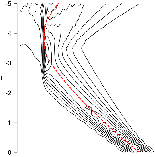
Figure 10: Still of a Movie where the coordinate time evolution [188] of a wave packet starting at the bottom and moving toward the classical singularity (vertical dotted line) is shown for different values of an ambiguity parameter. Some part of the wave packet bounces back (and deforms) according to the effective classical solution (dashed), but other parts penetrate to negative $\mu$. The farther away from $a=0$ the effective bounce happens, depending on the ambiguity parameter, the smaller the part penetrating to negative $\mu$ is. The coordinate time evolution represents a physical state obtained after integrating over $t$ [188]. The movie is available from the online version [91] of this article at http://relativity.livingreviews.org/Articles/lrr-2005-11/.

It is not clear in general that a wave function penetrating a classical singularity enters a new classical regime even if the volume becomes large again. For instance, there can be oscillations on small scales, i.e. violations of pre-classicality, picked up by the wave function when it travels through the classical singularity. As discussed in Sec. 5.6.5, the question of what conditions on a wave function to require for a classical regime is still open, but even if one can confidently say that there is such a new classical region does the question arise if time continues during the transition through the pure quantum regime. At least in the special model of a free massless scalar in isotropic cosmology the answer to both questions is affirmative, based on the availability of a physical inner product and quantum observables in this model [189].

Also related to this context is the question of unitary evolution. Even if one uses a selfadjoint constraint operator, unitary evolution is not guaranteed. First, the constraint splits into a time generator part containing derivatives or difference operators with respect to internal time and a source part containing, for instance, the matter Hamiltonian. It is then not guaranteed that the time generator will lead to unitary evolution. Secondly, it is not obvious in what inner product to measure unitarity since the constraint is formulated in the kinematical Hilbert space but the physical inner product is relevant for its solutions. This shows that the usual expectation of unitary evolution, commonly motivated by preservation of probability or normalization of a wave function in an absolute time parameter, is not reliable in quantum cosmology. It must be replaced by suitable conditions on relational probabilities computed from physical wave functions.

7.3 Determinism

Hat die Zeit nicht Zeit? (Does time not have time?)

Friedrich Nietzsche

Beyond Good and Evil

Loosely related to unitarity, but more general, is the concept of determinism. This is usually weakened in quantum mechanics anyway since in general one makes only probabilistic statements. Nevertheless, the wave function is determined at all times by its initial values, which is sometimes seen as the appropriate substitute for deterministic behavior. In loop quantum cosmology the situation again changes slightly since, as discussed in Sec. 5.6.6, the wave function may not be determined by the evolution equation everywhere, i.e. not at points of classical singularities, and instead acquire new conditions on its initial values. This could be seen as a form of indeterministic behavior, even though the values of a wave function at classical singularities would not have any effect on the behavior for non-degenerate configurations. (If they had such an effect, the evolution would be singular.) In this situation one deals with determinism in a background independent context, which requires a new view.

In fact, rather than interpreting the freedom of choosing values at classical singularities as indeterministic behavior, it seems more appropriate to see this as an example for deterministic behavior in a background independent theory. The internal time label $\mu$ first appears as a kinematical object through the eigenvalues of the triad operator (46). It then plays a role in the constraint equation (5.2.3) when formulated in the triad representation. Choosing internal time is just made for convenience, and it is the constraint equation which must be used to see if this choice makes sense in order to formulate evolution. This is indeed the case at non-zero $\mu$ where we obtain a difference operator in the evolution parameter. At zero $\mu$, however, the operator changes and does not allow us to determine the wave function there from previous values. Now, we can interpret this simply as a consequence of the constraint equation rejecting the internal time value $\mu=0$. The background independent evolution selects the values of internal time it needs to propagate a wave function uniquely. As it turns out, $\mu=0$ is not always necessary for this and thus simply decouples. In hindsight, one could already have split off $|0\rangle$ from the kinematical Hilbert space, thereby removing the classical singularity by hand. Since we did not do this, it is the evolution equation which tells us that this is happening anyway. Recall, however, that this is only one possible scenario obtained from a non-symmetric constraint. For the evolution (5.2.3) following from the symmetric constraint, no decoupling happens and $\mu=0$ is just like any other internal time value.

8 Research lines

Currently, the development of loop quantum cosmology proceeds along different lines, at all levels discussed before. We present here a list of the main ones, ordered by topics rather than importance or difficulty.

8.1 Conceptual issues

The list of conceptual issues is not much different from but equally pressing as in quantum gravity in general. Here, mainly the issue of time (its interpretation, different roles and explicit implementation into physics), the interpretation of the wave function in quantum theory, and technical as well as conceptual questions related to the physical inner product need to be addressed.

8.2 Mathematical development of models

The main open issue, requiring new insights at all levels, is that of inhomogeneities. While inhomogeneous models have been formulated and partly analyzed, the following tasks are still to be completed:

Exact models:

In particular the dynamics of inhomogeneous models is much more complicated to analyze than in homogeneous ones. Understanding may be improved by an interesting cross-relation with black holes. This allows one to see if the different ingredients and effects of a loop quantization fit together in a complete picture, which so far seems to be the case [152, 190, 191, 192, 162]. Moreover, the dynamics can possibly be simplified and understood better around slowly evolving horizons [193, 192]. Other horizon conditions are also being studied in related approaches [194, 195].

Consistency:

Not directly related to physical applications but equally important is the issue of consistency of the constraints. The constraint algebra trivializes in homogeneous models, but is much more restrictive with inhomogeneities. Here, the feasibility of formulating a consistent theory of quantum gravity can be tested in a treatable situation. Related to consistency of the algebra, at least at a technical level, is the question of whether or not quantum gravity can predict initial conditions for a universe, or at least restrict its set of solutions.

Relation between models and the full theory:

By strengthening the relation between models and the full theory, ideally providing a complete derivation of models, physical applications will be put on a much firmer footing. This is also necessary to understand better effects of reductions such as degeneracies between different concepts or partial backgrounds. One aspect not realized in models so far is the large amount of non-Abelian effects in the full theory which can be significant also in models [136].

Numerical quantum gravity:

Most systems of difference equations arising in loop quantum gravity are too complicated to solve exactly or even to analyze. Special techniques, such as those in [188, 166, 170, 189, 196] have to be developed so as to apply to more general systems. In particular for including inhomogeneities, both for solving equations and interpreting solutions, a new area of numerical quantum gravity has to be developed.

Perturbations:

If the relation between different models is known, as presently realized for isotropic within homogeneous models [178], one can formulate the less symmetric model perturbatively around the more symmetric one. This then provides a simpler formulation of the more complicated system, easing the analysis and uncovering new effects. In this context, also alternative methods to introduce approximate symmetries, based on coherent states as e.g. advocated in [197], exist.

Effective equations:

Finding effective equations which capture the quantum behavior of basic difference equations at least in some regimes will be most helpful for a general analysis. However, their derivation is much more complicated for inhomogeneous systems owing to the consistency issue. On the other hand, trying to derive them will provide important tests for the framework, in addition to giving rise to new applications.

8.3 Applications

Once available, equations for inhomogeneous systems have the prospect of applications such as

Structure formation:

There are diverse scenarios for the early universe with a potential for viable structure formation, which can only be checked with a reliable handle on inhomogeneities. This applies to inflaton models with loop effects, inflation models without inflaton, and the generation of structure before and subsequent propagation through a bounce.

Robustness:

All results obtained so far have to be regarded as preliminary and their validity in the presence of perturbative inhomogeneities has to be established. A detailed analysis of their robustness to quantization freedom such as ambiguities or choosing matter fields is still to be undertaken.

New effects:

Some cosmological issues which have not been addressed so far from loop quantum gravity and which most likely require inhomogeneities are: the initial state of the inflaton (Gaussianity) or the present acceleration of cosmic expansion. The latter could be a result of small, local quantum corrections adding up to a sizeable effect on the whole universe. From a technical point of view, contact to quantum gravity phenomenology in a particle physics context can be made (as initially in [117]).

Ansätze:

For the time being, those questions can be addressed preliminaryly by choosing suitable forms of inhomogeneous equations motivated by operators in full loop quantum gravity.

8.4 Homogeneous models

There are still several open areas in homogeneous models, which later can be extended to inhomogeneous ones:

Conceptual issues:

This has already been mentioned above. Isotropic models provide simpler settings to analyze, e.g., the physical inner product [198, 164, 189], observables, different interpretations of quantum aspects or the emergence of a classical world.

Effective equations:

Even in isotropic models effective equations have not yet been derived completely. A general scheme exists, shown to be analogous to standard effective action techniques [145], but it remains to be applied completely to quantum cosmology. This will then lead to a complete set of correction terms and their ranges of validity and importance. Also the question of whether an effective action for quantum cosmology exists and what its form is can be addressed.

Matter systems:

Matter systems provide a rich source of diverse scenarios, but a full analysis is yet to be done. This includes adding different kinds of fluids [199], fermions or anisotropy parameters (shear term).

8.5 Outlook

All these developments will certainly also aid and suggest developments in the full theory, and reciprocally be assisted by new ideas realized there. At the other side, guidance as well as means for testing can be expected from future observations.

Appendix

Appendix A Invariant connections

We first fix our notation by describing the additional structure provided by a given action of a symmetry group on a space manifold. This allows us to review the mathematical classification of principal fiber bundles carrying an action of a symmetry group, and their invariant connections.

A.1 Partial backgrounds

To describe a theory of connections we need to fix a principal fiber bundle $P(\Sigma,G,\pi)$ over the analytic base manifold $\Sigma$ with compact structure group $G$. Let $S<\mathrm{Aut}(P)$ be a Lie symmetry subgroup of bundle automorphisms acting on the principal fiber bundle $P$. Using the bundle projection $\pi\colon P\to\Sigma$ we get a symmetry operation of $S$ on $\Sigma$. For simplicity we will assume that all orbits of $S$ are of the same type. If necessary we will have to decompose the base manifold into several orbit bundles $\Sigma_{(F)}\subset\Sigma$, where $F\cong S_{x}$ is the isotropy subgroup of $S$ consisting of elements fixing a point $x$ of the orbit bundle $\Sigma_{(F)}$ (isotropy subgroups for different points in $\Sigma_{(F)}$ are not identical but conjugate to each other). This amounts to a special treatment of possible symmetry axes or centers.

By restricting ourselves to one fixed orbit bundle we fix an isotropy subgroup $F\leq S$ up to conjugacy, and we require that the action of $S$ on $\Sigma$ is such that the orbits are given by $S(x)\cong S/F$ for all $x\in\Sigma$. This will be the case if $S$ is compact but also in most other cases of physical interest. Moreover, we will have to assume later on that the coset space $S/F$ is reductive [200, 201], i.e. that ${\cal L}S$ can be written as a direct sum ${\cal L}S={\cal L}F\oplus{\cal L}F_{\perp}$ with $\mathrm{Ad}_{F}({\cal L}F_{\perp})\subset{\cal L}F_{\perp}$. If $S$ is semisimple, ${\cal L}F_{\perp}$ is the orthogonal complement of ${\cal L}F$ with respect to the Cartan–Killing metric on ${\cal L}S$. Further examples are provided by freely acting symmetry groups, in which case we have $F=\{1\}$, and semidirect products of the form $S=N\rtimes F$ where ${\cal L}F_{\perp}={\cal L}N$. The latter cases are relevant for homogeneous and isotropic cosmological models.

The base manifold can be decomposed as $\Sigma\cong\Sigma/S\times S/F$ where $\Sigma/S\cong B\subset\Sigma$ is the base manifold of the orbit bundle and can be realized as a submanifold $B$ of $\Sigma$ via a section in this bundle. As already noted in the main text, the action of a symmetry group on space introduces a partial background into the model. In particular, full diffeomorphism invariance is not preserved but reduced to diffeomorphisms only on the reduced manifold $B$. To see what kind of partial background we have in a model it is helpful to contrast the mathematical definition of symmetry actions with the physical picture.

To specify an action of a group on a manifold one has to give, for each group element, a map between space points satisfying certain conditions. Mathematically, each point is uniquely determined by labels, usually by coordinates in a chosen (local) coordinate system. The group action can then be written down in terms of maps of the coordinate charts, and there are compatibility conditions for maps expressed in different charts to ensure that the ensuing map on the manifold is coordinate independent. If we have active diffeomorphism invariance, however, individual points in space are not well-defined. This leads to the common view that geometrical observables such as the area of a surface are, for physical purposes, not actually defined by integrating over a submanifold simply in parameter form, but over subsets of space defined by the values of matter fields [202, 203]. Since matter fields are subject to diffeomorphisms just as the metric, area defined in such a manner is diffeomorphism invariant.

Similarly, orbits of the group action are not to be regarded as fixed submanifolds, but as being deformed by diffeomorphisms. Fixing a class of orbits filling the space manifold $\Sigma$ corresponds to selecting a special coordinate system adapted to the symmetry. For instance, in a spherically symmetric situation one usually chooses spherical coordinates $(r,\vartheta,\varphi)$, where $r>0$ labels the orbits and $\vartheta$ and $\varphi$ are angular coordinates and can be identified with some parameters of the symmetry group SO(3). In a Euclidean space the orbits can be embedded as spheres $S^{2}$ of constant curvature. Applying a diffeomorphism, however, will deform the spheres and they are in general only topological $S^{2}$. Physically, the orbits can be specified as level surfaces of matter fields, similar to specifying space points. This concept allows us to distinguish in a diffeomorphism invariant manner between curves (such as edges of spin networks) which are tangential and curves which are transversal to the group orbits.

It is, however, not possible to label single points in a given orbit in such a physical manner, simply because we could not introduce the necessary matter fields without destroying the symmetry. Thus we have to use the action of the symmetry group, which provides us with additional structure, to label the points, e.g. by using the angular coordinates in the example above. A similar role is played by the embedding of the reduced manifold $B$ into $\Sigma$ by choosing a section of the orbit bundle, which provides a base point for each orbit (a north pole in the example of spherical symmetry). This amounts to a partial fixing of the diffeomorphism invariance by allowing only diffeomorphisms which respect the additional structure. The reduced diffeomorphism constraint will then in general require only invariance with respect to diffeomorphisms of the manifold $B$.

In a reduced model, a partial fixing of the diffeomorphism invariance does not cause problems because all fields are constant along the orbits anyway. However, if we study symmetric states as generalized states of the full theory, as in Sec. 6, we inevitably have to break partially the diffeomorphism invariance. The distributional evaluation of symmetric states and the dual action of basic operators thus depends on the partial background provided by the symmetry.

A.2 Classification of symmetric principal fiber bundles

Fields which are invariant under the action of a symmetry group $S$ on space $\Sigma$ are defined by a set of linear equations for invariant field components. Nevertheless, finding invariant fields in gauge theories is not always straightforward since, in general, fields need to be invariant only up to gauge transformations which depend on the symmetry transformation. An invariant connection, for instance, satisfies the equation

$$s^{*}A=g(s)^{-1}Ag(s)+g(s)^{-1}\mathrm{d}g(s)$$ (67)

with a local gauge transformation $g(s)$ for each $s\in S$. These gauge transformations are not arbitrary since two symmetry transformations $s_{1}$ and $s_{2}$ applied one after another have to imply a gauge transformation with $g(s_{2}s_{1})$ related to $g(s_{1})$ and $g(s_{2})$. However, this does not simply amount to a homomorphism property and allowed maps $g\colon S\to G$ are not easily determined by group theory. Thus, even though for a known map $g$ one simply has to solve a system of linear equations for $A$, finding appropriate maps $g$ can be difficult. In most cases, the equations would not have any non-vanishing solution at all, which would certainly be insufficient for interesting reduced field theories.

In the earlier physical literature, invariant connections and other fields have indeed been determined by trial and error [204], but the same problem has been solved in the mathematical literature [200, 201, 205] in impressive generality. This uses the language of principal fiber bundles which already provides powerful techniques. Moreover, the problem of solving one system of equations for $A$ and $g(s)$ at the same time is split into two separate problems which allows a more systematic approach. The first step is to realize that a connection whose local 1-forms $A$ on $\Sigma$ are invariant up to gauge is equivalent to a connection 1-form $\omega$ defined on the full fiber bundle $P$ which satisfies the simple invariance conditions $s^{*}\omega=\omega$ for all $s\in S$. This is indeed simpler to analyze since we now have a set of linear equations for $\omega$ alone. However, even though hidden in the notation, the map $g\colon S\to G$ is still present. The invariance conditions for $\omega$ defined on $P$ are well-defined only if we know a lift from the original action of $S$ on the base manifold $\Sigma$ to the full bundle $P$. As with maps $g\colon S\to G$, there are several inequivalent choices for the lift which have to be determined. The advantage of this procedure is that this can be done by studying symmetric principal fiber bundles, i.e. principal fiber bundles carrying the action of a symmetry group, independently of the behavior of connections. In a second step, one can then ask what form invariant connections on a given symmetric principal fiber bundle have.

We now discuss the first step of determining lifts of the symmetry action of $S$ from $\Sigma$ to $P$. Given a point $x\in\Sigma$, the action of the isotropy subgroup $F$ yields a map $F\colon\pi^{-1}(x)\to\pi^{-1}(x)$ of the fiber over $x$ which commutes with the right action of $G$ on the bundle. To each point $p\in\pi^{-1}(x)$ we can assign a group homomorphism $\lambda_{p}\colon F\to G$ defined by $f(p)=:p\cdot\lambda_{p}(f)$ for all $f\in F$. To verify this we first note that commutativity of the action of $S<\mathrm{Aut}(P)$ with right multiplication of $G$ on $P$ implies that we have the conjugate homomorphism $\lambda_{p^{\prime}}=\mathrm{Ad}_{g^{-1}}\circ\lambda_{p}$ for a different point $p^{\prime}=p\cdot g$ in the same fiber:

$$p^{\prime}\cdot\lambda_{p^{\prime}}(f)=f(p\cdot g)=f(p)\cdot g=(p\cdot\lambda_{p}(f))\cdot g=p^{\prime}\cdot\mathrm{Ad}_{g^{-1}}\lambda_{p}(f)\,.$$

This yields

$$(f_{1}\circ f_{2})(p)=f_{1}(p\cdot\lambda_{p}(f_{2}))=(p\cdot\lambda_{p}(f_{2}))\cdot\mathrm{Ad}_{\lambda_{p}(f_{2})^{-1}}\lambda_{p}(f_{1})=p\cdot(\lambda_{p}(f_{1})\cdot\lambda_{p}(f_{2}))$$

demonstrating the homomorphism property. We thus obtain a map $\lambda\colon P\times F\to G,(p,f)\mapsto\lambda_{p}(f)$ obeying the relation $\lambda_{p\cdot g}=\mathrm{Ad}_{g^{-1}}\circ\lambda_{p}$.

Given a fixed homomorphism $\lambda\colon F\to G$, we can build the principal fiber subbundle

$$Q_{\lambda}(B,Z_{\lambda},\pi_{Q}):=\{p\in P_{|B}:\lambda_{p}=\lambda\}$$ (68)

over the base manifold $B$ which as structure group has the centralizer

$$Z_{\lambda}:=Z_{G}(\lambda(F))=\{g\in G:gf=fg\mbox{ for all }f\in\lambda(F)\}$$

of $\lambda(F)$ in $G$. $P_{|B}$ is the restricted fiber bundle over $B$. A conjugate homomorphism $\lambda^{\prime}=\mathrm{Ad}_{g^{-1}}\circ\lambda$ simply leads to an isomorphic fiber bundle.

The structure elements $[\lambda]$ and $Q$ classify symmetric principal fiber bundles according to the following theorem [205]:

Theorem 1

An $S$-symmetric principal fiber bundle $P(\Sigma,G,\pi)$ with isotropy subgroup $F\leq S$ of the action of $S$ on $\Sigma$ is uniquely characterized by a conjugacy class $[\lambda]$ of homomorphisms $\lambda\colon F\to G$ together with a reduced bundle $Q(\Sigma/S,Z_{G}(\lambda(F)),\pi_{Q})$.

Given two groups $F$ and $G$ we can make use of the relation [206]

$$\mathrm{Hom}(F,G)/\mathrm{Ad}\cong\mathrm{Hom}(F,T(G))/W(G)$$ (69)

in order to determine all conjugacy classes of homomorphisms $\lambda\colon F\to G$. Here, $T(G)$ is a maximal torus and $W(G)$ the Weyl group of $G$. Different conjugacy classes correspond to different sectors of the theory which can be interpreted as having different topological charge. In spherically symmetric electromagnetism, for instance, this is just magnetic charge [207, 8].

A.3 Classification of invariant connections

Now let $\omega$ be an $S$-invariant connection on the symmetric bundle $P$ classified by $([\lambda],Q)$, i.e. $s^{*}\omega=\omega$ for any $s\in S$. After restriction, $\omega$ induces a connection $\tilde{\omega}$ on the reduced bundle $Q$. Because of $S$-invariance of $\omega$ the reduced connection $\tilde{\omega}$ is a one-form on $Q$ with values in the Lie algebra of the reduced structure group. To see this, fix a point $p\in P$ and a vector $v$ in $T_{p}P$ such that $\pi_{*}v\in\sigma_{*}T_{\pi(p)}B$ where $\sigma$ is the embedding of $B$ into $\Sigma$. Such a vector, which does not have components along symmetry orbits, is fixed by the action of the isotropy group: $\mathrm{d}f(v)=v$. The pull back of $\omega$ by $f\in F$ applied to $v$ is by definition $f^{\star}\omega_{p}(v)=\omega_{f(p)}(\mathrm{d}f(v))=\omega_{f(p)}(v)$. Now using the fact that $f$ acts as gauge transformation in the fibers and observing the definition of $\lambda_{p}$ and the adjoint transformation of $\omega$, we obtain $\omega_{f(p)}(v)=\mathrm{Ad}_{\lambda_{p}(f)^{-1}}\omega_{p}(v)$. By assumption the connection $\omega$ is $S$-invariant implying $f^{\star}\omega_{p}(v)=\mathrm{Ad}_{\lambda_{p}(f)^{-1}}\omega_{p}(v)=\omega_{p}(v)$ for all $f\in F$. This shows that $\omega_{p}(v)\in{\cal L}Z_{G}(\lambda_{p}(F))$, and $\omega$ can be restricted to a connection on the bundle $Q_{\lambda}$ with structure group $Z_{\lambda}$.

Furthermore, using $\omega$ we can construct the linear map $\Lambda_{p}\colon{\cal L}S\to{\cal L}G,X\mapsto\omega_{p}(\tilde{X})$ for any $p\in P$. Here, $\tilde{X}$ is the vector field on $P$ given by $\tilde{X}(h):=\mathrm{d}(\exp(tX)^{\star}h)/\mathrm{d}t|_{t=0}$ for any $X\in{\cal L}S$ and $h\in C^{1}(P,{\mathbb{R}})$. For $X\in{\cal L}F$ the vector field $\tilde{X}$ is a vertical vector field, and we have $\Lambda_{p}(X)=\mathrm{d}\lambda_{p}(X)$ where $\mathrm{d}\lambda\colon{\cal L}F\to{\cal L}G$ is the derivative of the homomorphism defined above. This component of $\Lambda$ is therefore already given by the classifying structure of the principal fiber bundle. Using a suitable gauge, $\lambda$ can be held constant along $B$. The remaining components $\Lambda_{p}|_{{\cal L}F_{\perp}}$ yield information about the invariant connection $\omega$. They are subject to the condition

$$\Lambda_{p}(\mathrm{Ad}_{f}(X))=\mathrm{Ad}_{\lambda_{p}(f)}(\Lambda_{p}(X))\quad\mbox{ for }f\in F,X\in{\cal L}S$$ (70)

which follows from the transformation of $\omega$ under the adjoint representation and which provides a set of equations determining the form of the components $\Lambda$.

Keeping only the information characterizing $\omega$ we have, besides $\tilde{\omega}$, the scalar field $\tilde{\phi}\colon Q\to{\cal L}G\otimes{\cal L}F_{\perp}^{\star}$ which is determined by $\Lambda_{p}|_{{\cal L}F_{\perp}}$ and can be regarded as having $\dim{\cal L}F_{\perp}$ components of ${\cal L}G$-valued scalar fields. The reduced connection and the scalar field suffice to characterize an invariant connection [205]:

Theorem 2 (Generalized Wang Theorem)

Let $P(\Sigma,G)$ be an $S$-symmetric principal fiber bundle classified by $([\lambda],Q)$ according to Theorem 1, and let $\omega$ be an $S$-invariant connection on $P$.

Then the connection $\omega$ is uniquely classified by a reduced connection $\tilde{\omega}$ on $Q$ and a scalar field $\tilde{\phi}\colon Q\times{\cal L}F_{\perp}\to{\cal L}G$ obeying Eq. (70).

In general, $\tilde{\phi}$ transforms under some representation of the reduced structure group $Z_{\lambda}$: Its values lie in the subspace of ${\cal L}G$ determined by Eq. (70) and form a representation space for all group elements of $G$ (which act on $\Lambda$) whose action preserves the subspace. These are by definition precisely elements of the reduced group.

The connection $\omega$ can be reconstructed from its classifying structure $(\tilde{\omega},\tilde{\phi})$ as follows: according to the decomposition $\Sigma\cong B\times S/F$ we have

$$\omega=\tilde{\omega}+\omega_{S/F}\,,$$ (71)

where $\omega_{S/F}$ is given by $\Lambda\circ\iota^{\star}\theta_{\mathrm{MC}}$ in a gauge depending on the (local) embedding $\iota\colon S/F\hookrightarrow S$. Here $\theta_{\mathrm{MC}}$ is the Maurer–Cartan form on $S$ taking values in ${\cal L}S$. Through $\Lambda$, $\omega$ depends on $\lambda$ and $\tilde{\phi}$.

Appendix B Examples

With these general results we can now quickly derive the form of invariant connections for the cases studied in the main text.

B.1 Homogeneous models

In Bianchi models the transitive symmetry group acts freely on $\Sigma$, which implies that $\Sigma$ can locally be identified with the group manifold $S$. The three generators of ${\cal L}S$ will be denoted as $T_{I}$, $1\leq I\leq 3$, with relations $[T_{I},T_{J}]=C^{K}_{IJ}T_{K}$ where $C^{K}_{IJ}$ are the structure constants of ${\cal L}S$ fulfilling $C^{J}_{IJ}=0$ for class A models by definition. The Maurer–Cartan form on $S$ is given by $\theta_{\mathrm{MC}}=\omega^{I}T_{I}$ with left invariant one-forms $\omega^{I}$ on $S$ which fulfill the Maurer–Cartan equations

$$\mathrm{d}\omega^{I}=-{\textstyle\frac{1}{2}}C^{I}_{JK}\omega^{J}\wedge\omega^{K}\,.$$ (72)

Due to $F=\{1\}$ all homomorphisms $\lambda\colon F\to G$ are given by $1\mapsto 1$, and we can use the embedding $\iota=\mathrm{id}\colon S/F\hookrightarrow S$. An invariant connection then takes the form $A=\tilde{\phi}\circ\theta_{\mathrm{MC}}=\tilde{\phi}_{I}^{i}\tau_{i}\omega^{I}=A_{a}^{i}\tau_{i}\mathrm{d}x^{a}$ with matrices $\tau_{i}$ generating ${\cal L}\mathrm{SU}(2)$. The scalar field is given by $\tilde{\phi}\colon{\cal L}S\to{\cal L}G,T_{I}\mapsto\tilde{\phi}(T_{I})=:\tilde{\phi}^{i}_{I}\tau_{i}$ already in its final form, because condition (70) is empty for a trivial isotropy group.

Using left invariant vector fields $X_{I}$ obeying $\omega^{I}(X_{J})=\delta^{I}_{J}$ and with Lie brackets $[X_{I},X_{J}]=C^{K}_{IJ}X_{K}$ the momenta canonically conjugate to $A_{a}^{i}=\tilde{\phi}^{i}_{I}\omega^{I}_{a}$ can be written as $E^{a}_{i}=\sqrt{g_{0}}\,\tilde{p}^{I}_{i}X^{a}_{I}$ with $\tilde{p}^{I}_{i}$ being canonically conjugate to $\tilde{\phi}^{i}_{I}$. Here, $g_{0}=\det(\omega^{I}_{a})^{2}$ is the determinant of the left invariant metric $(g_{0})_{ab}:=\sum_{I}\omega^{I}_{a}\omega^{I}_{b}$ on $\Sigma$ which is used to provide the density weight of $E^{a}_{i}$. The symplectic structure can be derived from

$$\frac{1}{8\pi\gamma G}\int_{\Sigma}\mathrm{d}^{3}x\,\dot{A}^{i}_{a}E^{a}_{i}=\frac{1}{8\pi\gamma G}\int_{\Sigma}\mathrm{d}^{3}x\,\sqrt{g_{0}}\,\dot{\tilde{\phi}}{}^{i}_{I}\tilde{p}^{J}_{i}\omega^{I}(X_{J})=\frac{V_{0}}{8\pi\gamma G}\dot{\tilde{\phi}}{}^{i}_{I}\tilde{p}^{I}_{i}\,,$$

to obtain

$$\{\tilde{\phi}^{i}_{I},\tilde{p}^{J}_{j}\}=8\pi\gamma GV_{0}\delta^{i}_{j}\delta^{J}_{I}$$ (73)

with the volume $V_{0}:=\int_{\Sigma}\mathrm{d}^{3}x\sqrt{g_{0}}$ of $\Sigma$ measured with the invariant metric $g_{0}$.

It is convenient to absorb the coordinate volume $V_{0}$ into the fields by redefining $\phi^{i}_{I}:=V_{0}^{1/3}\tilde{\phi}^{i}_{I}$ and $p_{i}^{I}:=V_{0}^{2/3}\tilde{p}^{I}_{i}$. This makes the symplectic structure independent of $V_{0}$ in accordance with background independence. These redefined variables automatically appear in holonomies and fluxes through coordinate integrations.

B.2 Isotropic models

On Bianchi models additional symmetries can be imposed which corresponds to a further symmetry reduction and introduces non-trivial isotropy subgroups. These models with enhanced symmetry can be treated on an equal footing by writing the symmetry group as a semidirect product $S=N\rtimes_{\rho}F$, with the isotropy subgroup $F$ and the translational subgroup $N$ which is one of the Bianchi groups. Composition in this group is defined as $(n_{1},f_{1})(n_{2},f_{2}):=(n_{1}\rho(f_{1})(n_{2}),f_{1}f_{2})$ which depends on the group homomorphism $\rho\colon F\to\mathrm{Aut}N$ into the automorphism group of $N$ (which will be denoted by the same letter as the representation on $\mathrm{Aut}{\cal L}N$ used below). Inverse elements are given by $(n,f)^{-1}=(\rho(f^{-1})(n^{-1}),f^{-1})$. To determine the form of invariant connections we have to compute the Maurer–Cartan form on $S$ (using the usual notation):

$$\theta^{(S)}_{\mathrm{MC}}(n,f) = (n,f)^{-1}\mathrm{d}(n,f)=(\rho(f^{-1})(n^{-1}),f^{-1})(\mathrm{d}n,\mathrm{d}f)$$ (74)

$$= (\rho(f^{-1})(n^{-1})\rho(f^{-1})(\mathrm{d}n),f^{-1}\mathrm{d}f)=(\rho(f^{-1})(n^{-1}\mathrm{d}n),f^{-1}\mathrm{d}f)$$

$$= \left(\rho(f^{-1})(\theta^{(N)}_{\mathrm{MC}}(n)),\theta^{(F)}_{\mathrm{MC}}(f)\right)\,.$$

Here the Maurer–Cartan forms $\theta^{(N)}_{\mathrm{MC}}$ on $N$ and $\theta^{(F)}_{\mathrm{MC}}$ on $F$ appear. We then choose an embedding $\iota\colon S/F=N\hookrightarrow S$, which can most easily be done as $\iota\colon n\mapsto(n,1)$. Thus, $\iota^{*}\theta^{(S)}_{\mathrm{MC}}=\theta^{(N)}_{\mathrm{MC}}$, and a reconstructed connection takes the form $\tilde{\phi}\circ\iota^{*}\theta^{(S)}_{\mathrm{MC}}=\tilde{\phi}^{i}_{I}\omega^{I}\tau_{i}$ which is the same as for anisotropic models before (where now $\omega^{I}$ are left invariant one-forms on the translation group $N$). However, here $\tilde{\phi}$ is constrained by equation (70) and we get only a subset as isotropic connections.

To solve equation (70) we have to treat LRS (locally rotationally symmetric) models with a single rotational symmetry and isotropic models separately. In the first case we choose ${\cal L}F=\langle\tau_{3}\rangle$, whereas in the second case we have ${\cal L}F=\langle\tau_{1},\tau_{2},\tau_{3}\rangle$ ($\langle\cdot\rangle$ denotes the linear span). Eq. (70) can be written infinitesimally as

$$\tilde{\phi}(\mathrm{ad}_{\tau_{i}}(T_{I}))=\mathrm{ad}_{\mathrm{d}\lambda(\tau_{i})}\tilde{\phi}(T_{I})=[\mathrm{d}\lambda(\tau_{i}),\tilde{\phi}(T_{I})]$$

($i=3$ for LRS, $1\leq i\leq 3$ for isotropy). The $T_{I}$ are generators of ${\cal L}N={\cal L}F_{\perp}$, on which the isotropy subgroup $F$ acts by rotation, $\mathrm{ad}_{\tau_{i}}(T_{I})=\epsilon_{iIK}T_{K}$. This is the derivative of the representation $\rho$ defining the semidirect product $S$: conjugation on the left hand side of (70) is $\mathrm{Ad}_{(1,f)}(n,1)=(1,f)(n,1)(1,f^{-1})=(\rho(f)(n),1)$, which follows from the composition in $S$.

Next, we have to determine the possible conjugacy classes of homomorphisms $\lambda\colon F\to G$. For LRS models their representatives are given by

$$\lambda_{k}\colon\mathrm{U}(1)\to\mathrm{SU}(2),\exp t\tau_{3}\mapsto\exp kt\tau_{3}$$

for $k\in{\mathbb{N}}_{0}=\{0,1,\ldots\}$ (as will be shown in detail below for spherically symmetric connections). For the components $\tilde{\phi}^{i}_{I}$ of $\tilde{\phi}$ defined by $\tilde{\phi}(T_{I})=\tilde{\phi}^{i}_{I}\tau_{i}$, equation (70) takes the form $\epsilon_{3IK}\tilde{\phi}^{j}_{K}=k\epsilon_{3lj}\tilde{\phi}^{l}_{I}$. This has a non-trivial solution only for $k=1$, in which case $\tilde{\phi}$ can be written as

$$\tilde{\phi}_{1}=\tilde{a}\tau_{1}+\tilde{b}\tau_{2}\quad,\quad\tilde{\phi}_{2}=-\tilde{b}\tau_{1}+\tilde{a}\tau_{2}\quad,\quad\tilde{\phi}_{3}=\tilde{c}\tau_{3}$$

with arbitrary numbers $\tilde{a}$, $\tilde{b}$, $\tilde{c}$ (the factors of $2^{-\frac{1}{2}}$ are introduced for the sake of normalization). Their conjugate momenta take the form

$$\tilde{p}^{1}={\textstyle\frac{1}{2}}(\tilde{p}_{a}\tau_{1}+\tilde{p}_{b}\tau_{2})\quad,\quad\tilde{p}^{2}={\textstyle\frac{1}{2}}(-\tilde{p}_{b}\tau_{1}+\tilde{p}_{a}\tau_{2})\quad,\quad\tilde{p}^{3}=\tilde{p}_{c}\tau_{3}\,,$$

and the symplectic structure is given by

$$\{\tilde{a},\tilde{p}_{a}\}=\{\tilde{b},\tilde{p}_{b}\}=\{\tilde{c},\tilde{p}_{c}\}=8\pi\gamma GV_{0}$$

and vanishes in all other cases. There is remaining gauge freedom from the reduced structure group $Z_{\lambda}\cong\mathrm{U}(1)$ which rotates the pairs $(\tilde{a},\tilde{b})$ and $(\tilde{p}_{a},\tilde{p}_{b})$. Gauge invariant are then only $\sqrt{\tilde{a}^{2}+\tilde{b}^{2}}$ and its momentum $(\tilde{a}\tilde{p}_{a}+\tilde{b}\tilde{p}_{b})/\sqrt{\tilde{a}^{2}+\tilde{b}^{2}}$.

In the case of isotropic models we have only two homomorphisms $\lambda_{0}\colon\mathrm{SU}(2)\to\mathrm{SU}(2),f\mapsto 1$ and $\lambda_{1}=\mathrm{id}$ up to conjugation (to simplify notation we use the same letters for the homomorphisms as in the LRS case, which is justified by the fact that the LRS homomorphisms are restrictions of those appearing here). Equation (70) takes the form $\epsilon_{iIK}\tilde{\phi}^{j}_{K}=0$ for $\lambda_{0}$ without non-trivial solutions, and $\epsilon_{iIK}\tilde{\phi}^{j}_{K}=\epsilon_{ilj}\tilde{\phi}^{l}_{I}$ for $\lambda_{1}$. Each of the last equations has the same form as for LRS models with $k=1$, and their solution is $\tilde{\phi}^{i}_{I}=\tilde{c}\delta^{i}_{I}$ with an arbitrary $\tilde{c}$. In this case the conjugate momenta can be written as $\tilde{p}^{I}_{i}=\tilde{p}\delta^{I}_{i}$, and we have the symplectic structure $\{\tilde{c},\tilde{p}\}=\frac{8\pi}{3}G\gamma V_{0}$.

Thus, in both cases there is a unique non-trivial sector, and no topological charge appears. The symplectic structure can again be made independent of $V_{0}$ by redefining $a:=V_{0}^{1/3}\tilde{a}$, $b:=V_{0}^{1/3}\tilde{b}$, $c:=V_{0}^{1/3}\tilde{c}$ and $p_{a}:=V_{0}^{2/3}\tilde{p}_{a}$, $p_{b}:=V_{0}^{2/3}\tilde{p}_{b}$, $p_{c}:=V_{0}^{2/3}\tilde{p}_{c}$, $p:=V_{0}^{2/3}\tilde{p}$. If one computes the isotropic reduction of a Bianchi IX metric following from the left-invariant 1-forms of SU(2), one obtains a closed Friedmann–Robertson–Walker metric with scale factor $a=2\tilde{a}=2\sqrt{|\tilde{p}|}$ (see, e.g., [151] for the calculation). Thus, we obtain the identification (18) used in isotropic loop cosmology. (Such a normalization can only be obtained in curved models.)

B.3 Spherical symmetry

In the generic case (i.e., outside a symmetry center) of spherical symmetry we have $S=\mathrm{SU}(2)$, $F=\mathrm{U}(1)=\exp\langle\tau_{3}\rangle$ ($\langle\cdot\rangle$ denotes the linear span), and the connection form can be gauged to be

$$A_{S/F}=(\Lambda(\tau_{2})\sin\vartheta+\Lambda(\tau_{3})\cos\vartheta)\mathrm{d}\varphi+\Lambda(\tau_{1})\mathrm{d}\vartheta\,.$$ (75)

Here $(\vartheta,\varphi)$ are (local) coordinates on $S/F\cong S^{2}$ and as usually we use the basis elements $\tau_{i}$ of ${\cal L}S$. $\Lambda(\tau_{3})$ is given by $\mathrm{d}\lambda$, whereas $\Lambda(\tau_{1,2})$ are the scalar field components. Eq. (75) contains as special cases the invariant connections found in Ref. [204]. These are gauge equivalent by gauge transformations depending on the angular coordinates $(\vartheta,\varphi)$, i.e. they correspond to homomorphisms $\lambda$ which are not constant on the orbits of the symmetry group.

In order to specify the general form (75) further, the first step is again to find all conjugacy classes of homomorphisms $\lambda\colon F=\mathrm{U}(1)\to\mathrm{SU}(2)=G$. To do so we can make use of Eq. (69) to which end we need the following information about SU(2) (see, e.g., Ref. [206]): The standard maximal torus of SU(2) is given by

$$T(\mathrm{SU}(2))=\{\mathrm{diag}(z,z^{-1}):\,z\in\mathrm{U}(1)\}\cong\mathrm{U}(1)$$

and the Weyl group of SU(2) is the permutation group of two elements, $W(\mathrm{SU}(2))\cong S_{2}$, its generator acting on $T(\mathrm{SU}(2))$ by $\mathrm{diag}(z,z^{-1})\mapsto\mathrm{diag}(z^{-1},z)$.

All homomorphisms in $\mathrm{Hom}(\mathrm{U}(1),T(\mathrm{SU}(2)))$ are given by

$$\lambda_{k}\colon z\mapsto\mathrm{diag}(z^{k},z^{-k})$$

for any $k\in{\mathbb{Z}}$, and we have to divide out the action of the Weyl group leaving only the maps $\lambda_{k}$, $k\in{\mathbb{N}}_{0}$, as representatives of all conjugacy classes of homomorphisms. We see that spherically symmetric gravity has a topological charge taking values in ${\mathbb{N}}_{0}$ (but only if degenerate configurations are allowed, as we will see below).

We will represent $F$ as the subgroup $\exp\langle\tau_{3}\rangle<\mathrm{SU}(2)$ of the symmetry group $S$, and use the homomorphisms $\lambda_{k}\colon\exp t\tau_{3}\mapsto\exp kt\tau_{3}$ out of each conjugacy class. This leads to a reduced structure group $Z_{G}(\lambda_{k}(F))=\exp\langle\tau_{3}\rangle\cong\mathrm{U}(1)$ for $k\not=0$ and $Z_{G}(\lambda_{0}(F))=\mathrm{SU}(2)$ ($k=0$; this is the sector of manifestly invariant connections of Ref. [208]). The map $\Lambda|_{{\cal L}F}$ is given by $\mathrm{d}\lambda_{k}\colon\langle\tau_{3}\rangle\to{\cal L}G,\tau_{3}\mapsto k\tau_{3}$, and the remaining components of $\Lambda$, which give us the scalar field, are determined by $\Lambda(\tau_{1,\,2})\in{\cal L}G$ subject to Eq. (70) which here can be written as

$$\Lambda\circ\mathrm{ad}_{\tau_{3}}=\mathrm{ad}_{\mathrm{d}\lambda(\tau_{3})}\circ\Lambda\,.$$

Using $\mathrm{ad}_{\tau_{3}}\tau_{1}=\tau_{2}$ and $\mathrm{ad}_{\tau_{3}}\tau_{2}=-\tau_{1}$ we obtain

$$\Lambda(a_{0}\tau_{2}-b_{0}\tau_{1})=k(a_{0}[\tau_{3},\Lambda(\tau_{1})]+b_{0}[\tau_{3},\Lambda(\tau_{2})])\,,$$

where $a_{0}\tau_{1}+b_{0}\tau_{2}$, $a_{0},b_{0}\in{\mathbb{R}}$ is an arbitrary element of ${\cal L}F_{\perp}$. Since $a_{0}$ and $b_{0}$ are arbitrary, this is equivalent to the two equations

$$k[\tau_{3},\Lambda(\tau_{1})]=\Lambda(\tau_{2})\qquad\mbox{and}\qquad k[\tau_{3},\Lambda(\tau_{2})]=-\Lambda(\tau_{1})\,.$$

A general ansatz

$$\Lambda(\tau_{1})=a_{1}\tau_{1}+b_{1}\tau_{2}+c_{1}\tau_{3}\>,\quad\Lambda(\tau_{2})=a_{2}\tau_{1}+b_{2}\tau_{2}+c_{2}\tau_{3}$$

with arbitrary parameters $a_{i},b_{i},c_{i}\in{\mathbb{R}}$ yields

$$k(a_{1}\tau_{2}-b_{1}\tau_{1}) = a_{2}\tau_{1}+b_{2}\tau_{2}+c_{2}\tau_{3}\,,$$

$$k(-a_{2}\tau_{2}+b_{2}\tau_{1}) = a_{1}\tau_{1}+b_{1}\tau_{2}+c_{1}\tau_{3}$$

which have non-trivial solutions only if $k=1$, namely

$$b_{2}=a_{1}\>,\quad a_{2}=-b_{1}\quad\mbox{ and }\quad c_{1}=c_{2}=0\,.$$

The configuration variables of the system are the above fields $a,b,c\,\colon B\to{\mathbb{R}}$ of the $\mathrm{U}(1)$-connection form $A=c(x)\,\tau_{3}\,\mathrm{d}x$ on the one hand and the two scalar field components

$$\Lambda|_{\langle\tau_{1}\rangle}\colon B\to{\cal L}\mathrm{SU}(2),x\mapsto a(x)\tau_{1}+b(x)\tau_{2}$$

$$\qquad\qquad=\frac{1}{2}\left(\begin{array}[]{cc}0&-b(x)-ia(x)\\ b(x)-ia(x)&0\end{array}\right)=:\left(\begin{array}[]{cc}0&-\overline{w}(x)\\ w(x)&0\end{array}\right)$$

on the other hand. Under a local U(1)-gauge transformation $z(x)=\exp(t(x)\tau_{3})$ they transform as $c\mapsto c+\mathrm{d}t/\mathrm{d}x$ and $w(x)\mapsto\exp(-it)w$ which can be read off from

$$A \mapsto z^{-1}Az+z^{-1}\mathrm{d}z=A+\tau_{3}\mathrm{d}t\,,$$

$$\Lambda(\tau_{1}) \mapsto z^{-1}\Lambda(\tau_{1})z=\left(\begin{array}[]{cc}0&-\exp(it)\overline{w}\\ \exp(-it)w&0\end{array}\right)\,.$$

In order to obtain a standard symplectic structure (see Eq. (80) below), we reconstruct the general invariant connection form

$$A(x,\vartheta,\varphi) = A_{1}(x)\tau_{3}\mathrm{d}x+(A_{2}(x)\tau_{1}+A_{3}(x)\tau_{2})\mathrm{d}\vartheta$$

$$+(A_{2}(x)\tau_{2}-A_{3}(x)\tau_{1})\sin\vartheta\mathrm{d}\varphi+\cos\vartheta\,\mathrm{d}\varphi\,\tau_{3}\,.$$

An invariant densitized triad field is analogously given by

$$(E^{x},E^{\vartheta},E^{\varphi})=(E^{1}\sin\vartheta\,\tau_{3},{\textstyle\frac{1}{2}}\sin\vartheta(E^{2}\tau_{1}+E^{3}\tau_{2}),{\textstyle\frac{1}{2}}(E^{2}\tau_{2}-E^{3}\tau_{1}))$$ (79)

with coefficients $E^{I}$ canonically conjugate to $A_{I}$ ($E^{2}$ and $E^{3}$ are non-vanishing only for $k=1$). The symplectic structure

$$\{A_{I}(x),E^{J}(y)\}=2\gamma G\delta^{J}_{I}\delta(x,y)$$ (80)

can be derived by inserting the invariant expressions into $(8\pi\gamma G)^{-1}\int_{\Sigma}\mathrm{d}^{3}x\dot{A}_{a}^{i}E_{i}^{a}$.

Information about the topological charge $k$ can be found by expressing the volume in terms of the reduced triad coefficients $E^{I}$: using

$$\epsilon_{abc}\epsilon^{ijk}E_{i}^{a}E_{j}^{b}E_{k}^{c} = -2\epsilon_{abc}\mathrm{tr}(E^{a}[E^{b},E^{c}])$$

$$= \frac{3}{2}\sin^{2}\vartheta E^{1}\left((E^{2})^{2}+(E^{3})^{2}\right)$$

we have

$$V=\int_{\Sigma}\mathrm{d}^{3}x\sqrt{{\textstyle\frac{1}{6}}\left|\epsilon_{abc}\epsilon^{ijk}E_{a}^{i}E_{b}^{j}E_{c}^{k}\right|}=2\pi\int_{B}\mathrm{d}x\sqrt{|E^{1}|((E^{2})^{2}+(E^{3})^{2})}\,.$$ (82)

We can now see that in all the sectors with $k\not=1$ the volume vanishes because then $E^{2}=E^{3}=0$. All these degenerate sectors have to be rejected on physical grounds and we arrive at a unique sector of invariant connections given by the parameter $k=1$.

References

- [1] C. M. Will, The Confrontation between General Relativity and Experiment, Living Rev. Rel. 4 (2001) 4, [gr-qc/0103036], http://www.livingreviews.org/lrr-2001-4
- [2] S. W. Hawking and R. Penrose, The singularities of gravitational collapse and cosmology, Proc. Roy. Soc. Lond. A 314 (1970) 529–548
- [3] C. Rovelli, Loop Quantum Gravity, Living Rev. Rel. 1 (1998) 1, [gr-qc/9710008], http://www.livingreviews.org/Articles/Volume1/1998-1rovelli
- [4] A. Ashtekar and J. Lewandowski, Background independent quantum gravity: A status report, Class. Quantum Grav. 21 (2004) R53–R152, [gr-qc/0404018]
- [5] T. Thiemann, Introduction to Modern Canonical Quantum General Relativity, [gr-qc/0110034]
- [6] C. Rovelli, Quantum Gravity, Cambridge University Press, Cambridge, UK, 2004
- [7] M. Bojowald, Quantum Geometry and Symmetry, PhD thesis, RWTH Aachen, 2000, published by Shaker-Verlag, Aachen
- [8] M. Bojowald and H. A. Kastrup, Symmetry Reduction for Quantized Diffeomorphism Invariant Theories of Connections, Class. Quantum Grav. 17 (2000) 3009–3043, [hep-th/9907042]
- [9] M. Bojowald, Isotropic Loop Quantum Cosmology, Class. Quantum Grav. 19 (2002) 2717–2741, [gr-qc/0202077]
- [10] M. Bojowald, Loop quantum cosmology, In 100 Years of Relativity – Space-Time Structure: Einstein and Beyond, Ed. A. Ashtekar, World Scientific, Singapore, 2005, [gr-qc/0505057]
- [11] M. Bojowald, The Early Universe in Loop Quantum Cosmology, In Approaches to Quantum Gravity, VI Mexican School on Gravitation and Mathematical Physics, J. Phys.: Conference Series 24 (2005) 77–86, [gr-qc/0503020]
- [12] R. Vaas, The Inverted Big-Bang, Bild. Wiss. 2004N4 (2004) 50–55, [physics/0407071], translated by Amitabha Sen
- [13] M. Bojowald, Loop Quantum Cosmology: Recent Progress, In Proceedings of the International Conference on Gravitation and Cosmology (ICGC 2004), Cochin, India, Pramana 63 (2004) 765–776, [gr-qc/0402053]
- [14] M. Bojowald and H. A. Morales-Técotl, Cosmological applications of loop quantum gravity, In Proceedings of the Fifth Mexican School (DGFM): The Early Universe and Observational Cosmology, Lect. Notes Phys. 646 (2004) 421–462, Springer-Verlag, [gr-qc/0306008]
- [15] M. Bojowald, Quantum Gravity and the Big Bang, In Where Cosmology and Fundamental Physics Meet, IUFM, Marseille, Frontier Group, 2004, pp. 54–58, [astro-ph/0309478]
- [16] G. Date, Quantum Geometric Description of Cosmological Models, Mod. Phys. Lett. A 17 (2002) 967–976, [gr-qc/0205100]
- [17] H. Kodama, Specialization of Ashtekar’s Formalism to Bianchi Cosmology, Prog. Theor. Phys. 80 (1988) 1024–1040
- [18] H. Kodama, Holomorphic wave function of the Universe, Phys. Rev. D 42 (1990) 2548–2565
- [19] S. Alexander, J. Malecki, and L. Smolin, Quantum Gravity and Inflation, Phys. Rev. D 70 (2004) 044025, [hep-th/0309045]
- [20] L. Freidel and L. Smolin, The linearization of the Kodama state, Class. Quant. Grav. 21 (2004) 3831–3844, [hep-th/0310224]
- [21] J. Malecki, Inflationary Quantum Cosmology: General Framework and Exact Bianchi I Solution, Phys. Rev. D 70 (2004) 084040, [gr-qc/0407114]
- [22] S. Alexander, A Quantum Gravitational Relaxation of The Cosmological Constant, Phys. Lett. B 629 (2005) 53–59, [hep-th/0503146]
- [23] H. Nicolai, K. Peeters, and M. Zamaklar, Loop quantum gravity: an outside view, Class. Quantum Grav. 22 (2005) R193–R247, [hep-th/0501114]
- [24] A. Ashtekar, Quantum Geometry and Gravity: Recent Advances, In Proceedings of the 16th International Conference on General Relativity and Gravitation, 2001, [gr-qc/0112038]
- [25] A. Ashtekar, Quantum Geometry In Action: Big Bang and Black Holes, In Proceedings of the conference “Graphs and Patterns in Mathematics and Theoretical Physics”, 2002, [math-ph/0202008]
- [26] C. Rovelli, A dialog on quantum gravity, Int. J. Mod. Phys. D 12 (2003) 1509–1528, [hep-th/0310077]
- [27] L. Smolin, An invitation to loop quantum gravity, [hep-th/0408048]
- [28] A. Perez, Introduction to Loop Quantum Gravity and Spin Foams, In II International Conference of Fundamental Interactions, Pedra Azul, Brazil, 2004, [gr-qc/0409061]
- [29] R. Vaas, Beyond Space And Time, Bild. Wiss. 12 (2003) 50–56, [physics/0401128], translated by Amitabha Sen
- [30] A. Corichi and A. Hauser, Bibliography of Publications related to Classical Self-dual variables and Loop Quantum Gravity, [gr-qc/0509039]
- [31] R. Arnowitt, S. Deser, and C. W. Misner, The Dynamics of General Relativity, Wiley, New York, 1962
- [32] P. A. M. Dirac, Lectures on Quantum Mechanics, Yeshiva Press, 1969
- [33] A. Ashtekar, New Variables for Classical and Quantum Gravity, Phys. Rev. Lett. 57 (1986) 2244–2247
- [34] A. Ashtekar, New Hamiltonian Formulation of General Relativity, Phys. Rev. D 36 (1987) 1587–1602
- [35] J. F. Barbero G., Real Ashtekar Variables for Lorentzian Signature Space-Times, Phys. Rev. D 51 (1995) 5507–5510, [gr-qc/9410014]
- [36] G. Immirzi, Real and Complex Connections for Canonical Gravity, Class. Quantum Grav. 14 (1997) L177–L181
- [37] C. Rovelli and L. Smolin, Loop Space Representation of Quantum General Relativity, Nucl. Phys. B 331 (1990) 80–152
- [38] H. Sahlmann, Some Comments on the Representation Theory of the Algebra Underlying Loop Quantum Gravity, [gr-qc/0207111]
- [39] H. Sahlmann, When Do Measures on the Space of Connections Support the Triad Operators of Loop Quantum Gravity?, [gr-qc/0207112]
- [40] A. Okołów and J. Lewandowski, Diffeomorphism covariant representations of the holonomy-flux star-algebra, Class. Quantum Grav. 20 (2003) 3543–3568, [gr-qc/0302059]
- [41] H. Sahlmann and T. Thiemann, On the superselection theory of the Weyl algebra for diffeomorphism invariant quantum gauge theories, [gr-qc/0302090]
- [42] C. Fleischhack, Representations of the Weyl Algebra in Quantum Geometry, [math-ph/0407006]
- [43] J. Lewandowski, A. Okołów, H. Sahlmann, and T. Thiemann, Uniqueness of diffeomorphism invariant states on holonomy-flux algebras, [gr-qc/0504147]
- [44] C. Rovelli and L. Smolin, Spin Networks and Quantum Gravity, Phys. Rev. D 52 (1995) 5743–5759
- [45] J. Lewandowski, E. T. Newman, and C. Rovelli, Variations of the Parallel Propagator and Holonomy Operator and the Gauss Law Constraint, J. Math. Phys. 34 (1993) 4646–4654
- [46] A. Ashtekar and J. Lewandowski, Quantum Theory of Geometry I: Area Operators, Class. Quantum Grav. 14 (1997) A55–A82, [gr-qc/9602046]
- [47] A. Ashtekar, J. C. Baez, A. Corichi, and K. Krasnov, Quantum Geometry and Black Hole Entropy, Phys. Rev. Lett. 80 (1998) 904–907, [gr-qc/9710007]
- [48] A. Ashtekar, J. C. Baez, and K. Krasnov, Quantum Geometry of Isolated Horizons and Black Hole Entropy, Adv. Theor. Math. Phys. 4 (2000) 1–94, [gr-qc/0005126]
- [49] M. Domagala and J. Lewandowski, Black hole entropy from Quantum Geometry, Class. Quantum Grav. 21 (2004) 5233–5243, [gr-qc/0407051]
- [50] K. A. Meissner, Black hole entropy in Loop Quantum Gravity, Class. Quantum Grav. 21 (2004) 5245–5251, [gr-qc/0407052]
- [51] A. Ashtekar, A. Corichi, and J. Zapata, Quantum Theory of Geometry III: Non-commutativity of Riemannian Structures, Class. Quantum Grav. 15 (1998) 2955–2972, [gr-qc/9806041]
- [52] R. Giles, The reconstruction of gauge potentials from Wilson loops, Phys. Rev. D 24 (1981) 2160–2168
- [53] A. Ashtekar, J. Lewandowski, D. Marolf, J. Mourão, and T. Thiemann, Quantization of Diffeomorphism Invariant Theories of Connections with Local Degrees of Freedom, J. Math. Phys. 36 (1995) 6456–6493, [gr-qc/9504018]
- [54] A. Ashtekar and J. Lewandowski, Projective Techniques and Functional Integration for Gauge Theories, J. Math. Phys. 36 (1995) 2170–2191
- [55] D. Marolf and J. M. Mourão, On the support of the Ashtekar-Lewandowski measure, Commun. Math. Phys. 170 (1995) 583–606, [hep-th/9403112]
- [56] C. Rovelli and L. Smolin, Discreteness of Area and Volume in Quantum Gravity, Nucl. Phys. B 442 (1995) 593–619, [gr-qc/9411005], Erratum: Nucl. Phys. B 456 (1995) 753
- [57] A. Ashtekar and J. Lewandowski, Quantum Theory of Geometry II: Volume Operators, Adv. Theor. Math. Phys. 1 (1997) 388–429, [gr-qc/9711031]
- [58] R. Loll, Discrete Approaches to Quantum Gravity in Four Dimensions, Living Rev. Rel. 1 (1998) 13, [gr-qc/9805049], http://www.livingreviews.org/lrr-1998-13
- [59] R. Loll, Simplifying the Spectral Analysis of the Volume Operator, Nucl. Phys. B 500 (1997) 405–420, [gr-qc/9706038]
- [60] R. De Pietri and C. Rovelli, Geometry Eigenvalues and the Scalar Product from Recoupling Theory in Loop Quantum Gravity, Phys. Rev. D 54 (1996) 2664–2690
- [61] R. De Pietri, Spin Networks and Recoupling in Loop Quantum Gravity, Nucl. Phys. Proc. Suppl. 57 (1997) 251–254, [gr-qc/9701041]
- [62] J. Brunnemann and T. Thiemann, Simplification of the Spectral Analysis of the Volume Operator in Loop Quantum Gravity, [gr-qc/0405060]
- [63] T. Thiemann, A Length Operator for Canonical Quantum Gravity, J. Math. Phys. 39 (1998) 3372–3392, [gr-qc/9606092]
- [64] T. Thiemann, QSD V: Quantum Gravity as the Natural Regulator of Matter Quantum Field Theories, Class. Quantum Grav. 15 (1998) 1281–1314, [gr-qc/9705019]
- [65] T. Thiemann, Quantum Spin Dynamics (QSD), Class. Quantum Grav. 15 (1998) 839–873, [gr-qc/9606089]
- [66] C. Rovelli and L. Smolin, The physical Hamiltonian in nonperturbative quantum gravity, Phys. Rev. Lett. 72 (1994) 446–449, [gr-qc/9308002]
- [67] L. Smolin, The Classical Limit and the Form of the Hamiltonian Constraint in Non-Perturbative Quantum General Relativity, [gr-qc/9609034]
- [68] M. Gaul and C. Rovelli, A generalized Hamiltonian Constraint Operator in Loop Quantum Gravity and its simplest Euclidean Matrix Elements, Class. Quantum Grav. 18 (2001) 1593–1624, [gr-qc/0011106]
- [69] F. Hinterleitner and S. Major, Isotropic Loop Quantum Cosmology with Matter II: The Lorentzian Constraint, Phys. Rev. D 68 (2003) 124023, [gr-qc/0309035]
- [70] T. Thiemann, Anomaly-Free Formulation of Non-Perturbative, Four-Dimensional Lorentzian Quantum Gravity, Phys. Lett. B 380 (1996) 257–264, [gr-qc/9606088]
- [71] K. V. Kuchař, Time and interpretations of quantum gravity, In Proceedings of the 4th Canadian Conference on General Relativity and Relativistic Astrophysics, Ed. G. Kunstatter, D. E. Vincent, and J. G. Williams, World Scientific, Singapore, 1992.
- [72] P. Anninos, Computational Cosmology: From the Early Universe to the Large Scale Structure, Living Rev. Rel. 4 (2001) 2, [gr-qc/0108083], http://www.livingreviews.org/lrr-2001-2
- [73] A. Ashtekar, M. Bojowald, and J. Lewandowski, Mathematical structure of loop quantum cosmology, Adv. Theor. Math. Phys. 7 (2003) 233–268, [gr-qc/0304074]
- [74] A. Borde, A. H. Guth, and A. Vilenkin, Inflationary spacetimes are not past-complete, Phys. Rev. Lett. 90 (2003) 151301, [gr-qc/0110012]
- [75] B. S. DeWitt, Quantum Theory of Gravity. I. The Canonical Theory, Phys. Rev. 160 (1967) 1113–1148
- [76] N. Kontoleon and D. L. Wiltshire, Operator ordering and consistency of the wavefunction of the Universe, Phys. Rev. D 59 (1999) 063513, [gr-qc/9807075]
- [77] A. Ashtekar, S. Fairhurst, and J. Willis, Quantum Gravity, Shadow States, and Quantum Mechanics, Class. Quant. Grav. 20 (2003) 1031–1062, [gr-qc/0207106]
- [78] M. Bojowald, Inverse Scale Factor in Isotropic Quantum Geometry, Phys. Rev. D 64 (2001) 084018, [gr-qc/0105067]
- [79] M. Bojowald, Quantization ambiguities in isotropic quantum geometry, Class. Quantum Grav. 19 (2002) 5113–5130, [gr-qc/0206053]
- [80] P. Singh, Effective State Metamorphosis in Semi-Classical Loop Quantum Cosmology, Class. Quantum Grav. 22 (2005) 4203–4216, [gr-qc/0502086]
- [81] J. E. Lidsey, Early Universe Dynamics in Semi-Classical Loop Quantum Cosmology, JCAP 0412 (2004) 007, [gr-qc/0411124]
- [82] E. J. Copeland, J. E. Lidsey, and S. Mizuno, Correspondence between Loop-inspired and Braneworld Cosmology, [gr-qc/0510022]
- [83] P. Singh and A. Toporensky, Big Crunch Avoidance in Semi-Classical Loop Quantum Cosmology, Phys. Rev. D 69 (2004) 104008, [gr-qc/0312110]
- [84] M. Bojowald, Inflation from quantum geometry, Phys. Rev. Lett. 89 (2002) 261301, [gr-qc/0206054]
- [85] M. Bojowald and K. Vandersloot, Loop quantum cosmology, boundary proposals, and inflation, Phys. Rev. D 67 (2003) 124023, [gr-qc/0303072]
- [86] M. Bojowald, R. Maartens, and P. Singh, Loop Quantum Gravity and the Cyclic Universe, Phys. Rev. D 70 (2004) 083517, [hep-th/0407115]
- [87] G. V. Vereshchagin, Qualitative Approach to Semi-Classical Loop Quantum Cosmology, JCAP 07 (2004) 013, [gr-qc/0406108]
- [88] G. Date and G. M. Hossain, Genericity of Big Bounce in isotropic loop quantum cosmology, Phys. Rev. Lett. 94 (2005) 011302, [gr-qc/0407074]
- [89] G. Date, Absence of the Kasner singularity in the effective dynamics from loop quantum cosmology, Phys. Rev. D 71 (2005) 127502, [gr-qc/0505002]
- [90] G. Date and G. M. Hossain, Genericity of inflation in isotropic loop quantum cosmology, Phys. Rev. Lett. 94 (2005) 011301, [gr-qc/0407069]
- [91] M. Bojowald, Loop Quantum Cosmology, Living Rev. Relativity 8 (2005) 11, http://relativity.livingreviews.org/Articles/lrr-2005-11/
- [92] M. Bojowald, J. E. Lidsey, D. J. Mulryne, P. Singh, and R. Tavakol, Inflationary Cosmology and Quantization Ambiguities in Semi-Classical Loop Quantum Gravity, Phys. Rev. D 70 (2004) 043530, [gr-qc/0403106]
- [93] S. Tsujikawa, P. Singh, and R. Maartens, Loop quantum gravity effects on inflation and the CMB, Class. Quantum Grav. 21 (2004) 5767–5775, [astro-ph/0311015]
- [94] A. Jones and A. Lasenby, The Cosmic Microwave Background, Living Rev. Rel. 1 (1998) 11, http://www.livingreviews.org/lrr-1998-11
- [95] A. Ashtekar, P. Singh, and P. Vandersloot, in preparation
- [96] J. E. Lidsey, D. J. Mulryne, N. J. Nunes, and R. Tavakol, Oscillatory Universes in Loop Quantum Cosmology and Initial Conditions for Inflation, Phys. Rev. D 70 (2004) 063521, [gr-qc/0406042]
- [97] J. Khoury, B. A. Ovrut, P. J. Steinhardt, and N. Turok, The Ekpyrotic Universe: Colliding Branes and the Origin of the Hot Big Bang, Phys. Rev. D 64 (2001) 123522, [hep-th/0103239]
- [98] R. Maartens, Brane-World Gravity, Living Rev. Rel. 7 (2004) 7, [gr-qc/0312059], http://www.livingreviews.org/lrr-2004-7
- [99] G. F. R. Ellis and R. Maartens, The Emergent Universe: inflationary cosmology with no singularity, Class. Quant. Grav. 21 (2004) 223–232, [gr-qc/0211082]
- [100] G. F. R. Ellis, J. Murugan, and C. G. Tsagas, The Emergent Universe: An Explicit Construction, Class. Quant. Grav. 21 (2004) 233–250, [gr-qc/0307112]
- [101] D. J. Mulryne, R. Tavakol, J. E. Lidsey, and G. F. R. Ellis, An emergent universe from a loop, Phys. Rev. D 71 (2005) 123512, [astro-ph/0502589]
- [102] M. Bojowald, Original Questions, Nature 436 (2005) 920–921
- [103] D. H. Coule, Contrasting Quantum Cosmologies, [gr-qc/0312045]
- [104] D. H. Coule, Quantum Cosmological Models, Class. Quantum Grav. 22 (2005) R125–R166, [gr-qc/0412026]
- [105] G. M. Hossain, On Energy Conditions and Stability in Effective Loop Quantum Cosmology, Class. Quant. Grav. 22 (2005) 2653–2670, [gr-qc/0503065]
- [106] V. A. Belinskii, I. M. Khalatnikov, and E. M. Lifschitz, A general solution of the Einstein equations with a time singularity, Adv. Phys. 13 (1982) 639–667
- [107] E. Kasner, Geometrical Theorems on Einstein’s Cosmological Equations, Am. J. Math. 43 (1921) 217
- [108] M. Bojowald, Homogeneous loop quantum cosmology, Class. Quantum Grav. 20 (2003) 2595–2615, [gr-qc/0303073]
- [109] M. Bojowald, G. Date, and K. Vandersloot, Homogeneous loop quantum cosmology: The role of the spin connection, Class. Quantum Grav. 21 (2004) 1253–1278, [gr-qc/0311004]
- [110] C. W. Misner, The Isotropy of the Universe, Astrophys. J. 151 (1968) 431–457
- [111] C. W. Misner, Mixmaster Universe, Phys. Rev. Lett. 22 (1969) 1071–1074
- [112] B. Berger, Numerical Approaches to Spacetime Singularities, Living Rev. Relativity 5 (2002) 1, [gr-qc/0201056], http://www.livingreviews.org/lrr-2002-1
- [113] M. Bojowald and G. Date, Quantum suppression of the generic chaotic behavior close to cosmological singularities, Phys. Rev. Lett. 92 (2004) 071302, [gr-qc/0311003]
- [114] M. Bojowald, G. Date, and G. M. Hossain, The Bianchi IX model in loop quantum cosmology, Class. Quantum Grav. 21 (2004) 3541–3569, [gr-qc/0404039]
- [115] A. D. Rendall, The nature of spacetime singularities, In 100 Years of Relativity – Space-Time Structure: Einstein and Beyond, Ed. A. Ashtekar, World Scientific, Singapore, 2005, [gr-qc/0503112]
- [116] H. Sahlmann, T. Thiemann, and O. Winkler, Coherent States for Canonical Quantum General Relativity and the Infinite Tensor Product Extension, Nucl. Phys. B 606 (2001) 401–440, [gr-qc/0102038]
- [117] M. Bojowald, H. Morales-Técotl, and H. Sahlmann, On Loop Quantum Gravity Phenomenology and the Issue of Lorentz Invariance, Phys. Rev. D 71 (2005) 084012, [gr-qc/0411101]
- [118] R. Gambini and J. Pullin, Nonstandard optics from quantum spacetime, Phys. Rev. D 59 (1999) 124021, [gr-qc/9809038]
- [119] J. Alfaro, H. A. Morales-Técotl, and L. F. Urrutia, Quantum gravity corrections to neutrino propagation, Phys. Rev. Lett. 84 (2000) 2318–2321, [gr-qc/9909079]
- [120] J. Alfaro, H. A. Morales-Técotl, and L. F. Urrutia, Loop quantum gravity and light propagation, Phys. Rev. D 65 (2002) 103509, [hep-th/0108061]
- [121] H. Sahlmann and T. Thiemann, Towards the QFT on Curved Spacetime Limit of QGR. I: A General Scheme, [gr-qc/0207030]
- [122] H. Sahlmann and T. Thiemann, Towards the QFT on Curved Spacetime Limit of QGR. II: A Concrete Implementation, [gr-qc/0207031]
- [123] J. J. Halliwell and S. W. Hawking, Origin of Structure in the Universe, Phys. Rev. D 31 (1985) 1777–1791
- [124] T. Thiemann and H. A. Kastrup, Canonical Quantization of Spherically Symmetric Gravity in Ashtekar’s Self-Dual Representation, Nucl. Phys. B 399 (1993) 211–258, [gr-qc/9310012]
- [125] H. A. Kastrup and T. Thiemann, Spherically Symmetric Gravity as a Completely Integrable System, Nucl. Phys. B 425 (1994) 665–686, [gr-qc/9401032]
- [126] M. Bojowald and R. Swiderski, Spherically Symmetric Quantum Geometry: Hamiltonian Constraint, [gr-qc/0511108]
- [127] M. Bojowald, Spherically Symmetric Quantum Geometry: States and Basic Operators, Class. Quantum Grav. 21 (2004) 3733–3753, [gr-qc/0407017]
- [128] M. Bojowald and R. Swiderski, The Volume Operator in Spherically Symmetric Quantum Geometry, Class. Quantum Grav. 21 (2004) 4881–4900, [gr-qc/0407018]
- [129] M. Bojowald, Loop Quantum Cosmology III: Wheeler-DeWitt Operators, Class. Quantum Grav. 18 (2001) 1055–1070, [gr-qc/0008052]
- [130] M. Bojowald, Quantum Riemannian Geometry and Black Holes, to appear
- [131] G. M. Hossain, Primordial Density Perturbation in Effective Loop Quantum Cosmology, Class. Quantum Grav. 22 (2005) 2511–2532, [gr-qc/0411012]
- [132] S. Hofmann and O. Winkler, The Spectrum of Fluctuations in Inflationary Quantum Cosmology, [astro-ph/0411124]
- [133] T. Padmanabhan, Acceptable Density Perturbations From Inflation due to Quantum Gravitational Damping, Phys. Rev. Lett. 60 (1988) 2229–2230
- [134] T. Padmanabhan, T. R. Seshadri, and T. P. Singh, Making inflation work: Damping of density perturbations due to Planck energy cutoff, Phys. Rev. D 39 (1989) 2100–2107
- [135] M. Bojowald, Loop Quantum Cosmology: II. Volume Operators, Class. Quantum Grav. 17 (2000) 1509–1526, [gr-qc/9910104]
- [136] M. Bojowald, Degenerate Configurations, Singularities and the Non-Abelian Nature of Loop Quantum Gravity, Class. Quantum Grav. 23 (2006) to appear, [gr-qc/0508118]
- [137] M. Bojowald, Loop Quantum Cosmology IV: Discrete Time Evolution, Class. Quantum Grav. 18 (2001) 1071–1088, [gr-qc/0008053]
- [138] K. Vandersloot, On the Hamiltonian Constraint of Loop Quantum Cosmology, Phys. Rev. D 71 (2005) 103506, [gr-qc/0502082]
- [139] M. Bojowald, The Semiclassical Limit of Loop Quantum Cosmology, Class. Quantum Grav. 18 (2001) L109–L116, [gr-qc/0105113]
- [140] G. Date and G. M. Hossain, Effective Hamiltonian for Isotropic Loop Quantum Cosmology, Class. Quantum Grav. 21 (2004) 4941–4953, [gr-qc/0407073]
- [141] K. Banerjee and G. Date, Discreteness Corrections to the Effective Hamiltonian of Isotropic Loop Quantum Cosmology, Class. Quant. Grav. 22 (2005) 2017–2033, [gr-qc/0501102]
- [142] G. M. Hossain, Large volume quantum correction in loop quantum cosmology: Graviton illusion?, [gr-qc/0504125]
- [143] A. Shojai and F. Shojai, Causal Loop Quantum Gravity and Cosmological Solutions, Europhys. Lett. 71 (2005) 886, [gr-qc/0409020]
- [144] A. Ashtekar and T. A. Schilling, Geometrical Formulation of Quantum Mechanics, pages 23–65, Springer, New York, 1999, [gr-qc/9706069]
- [145] M. Bojowald and A. Skirzewski, Effective Equations of Motion for Quantum Systems pages math–ph/0511043
- [146] A. Ashtekar, M. Bojowald, and J. Willis, in preparation
- [147] J. Willis, On the Low-Energy Ramifications and a Mathematical Extension of Loop Quantum Gravity, PhD thesis, The Pennsylvania State University, 2004
- [148] P. Singh and K. Vandersloot, Semi-classical States, Effective Dynamics and Classical Emergence in Loop Quantum Cosmology, Phys. Rev. D 72 (2005) 084004, [gr-qc/0507029]
- [149] G. F. R. Ellis and M. A. H. MacCallum, A Class of Homogeneous Cosmological Models, Commun. Math. Phys. 12 (1969) 108–141
- [150] A. Ashtekar and J. Samuel, Bianchi Cosmologies: The Role of Spatial Topology, Class. Quantum Grav. 8 (1991) 2191–2215
- [151] M. Bojowald, Loop Quantum Cosmology: I. Kinematics, Class. Quantum Grav. 17 (2000) 1489–1508, [gr-qc/9910103]
- [152] A. Ashtekar and M. Bojowald, Quantum Geometry and the Schwarzschild Singularity, Class. Quantum Grav. 23 (2006) 391–411, [gr-qc/0509075]
- [153] A. Einstein and N. Rosen, On Gravitational Waves, J. Franklin Inst. 233 (1937) 43
- [154] J. Bicák and B. Schmidt, Asymptotically flat radiative space-times with boost-rotation symmetry: The general structure, Phys. Rev. D 40 (1989) 1827–1853
- [155] V. Husain and O. Winkler, On singularity resolution in quantum gravity, Phys. Rev. D 69 (2004) 084016, [gr-qc/0312094]
- [156] K. Giesel and T. Thiemann, Consistency Check on Volume and Triad Operator Quantisation in Loop Quantum Gravity I, [gr-qc/0507036]
- [157] L. Modesto, The Kantowski-Sachs Space-Time in Loop Quantum Gravity, [gr-qc/0411032]
- [158] J. Brunnemann and T. Thiemann, Unboundedness of Triad-Like Operators in Loop Quantum Gravity, [gr-qc/0505033]
- [159] M. Bojowald and G. Date, Consistency conditions for fundamentally discrete theories, Class. Quantum Grav. 21 (2004) 121–143, [gr-qc/0307083]
- [160] S. W. Hawking and G. F. R. Ellis, The Large Scale Structure of Space-Time, Cambridge University Press, 1973
- [161] M. Bojowald, Absence of a Singularity in Loop Quantum Cosmology, Phys. Rev. Lett. 86 (2001) 5227–5230, [gr-qc/0102069]
- [162] M. Bojowald, Non-singular black holes and degrees of freedom in quantum gravity, Phys. Rev. Lett. 95 (2005) 061301, [gr-qc/0506128]
- [163] J. M. Velhinho, Comments on the kinematical structure of loop quantum cosmology, Class. Quantum Grav. 21 (2004) L109–L113, [gr-qc/0406008]
- [164] K. Noui, A. Perez, and K. Vandersloot, On the Physical Hilbert Space of Loop Quantum Cosmology, Phys. Rev. D 71 (2005) 044025, [gr-qc/0411039]
- [165] M. Bojowald, Dynamical Initial Conditions in Quantum Cosmology, Phys. Rev. Lett. 87 (2001) 121301, [gr-qc/0104072]
- [166] D. Cartin, G. Khanna, and M. Bojowald, Generating function techniques for loop quantum cosmology, Class. Quantum Grav. 21 (2004) 4495–4509, [gr-qc/0405126]
- [167] D. Cartin and G. Khanna, Absence of pre-classical solutions in Bianchi I loop quantum cosmology, Phys. Rev. Lett. 94 (2005) 111302, [gr-qc/0501016]
- [168] T. Hertog and G. T. Horowitz, Holographic Description of AdS Cosmologies, JHEP 0504 (2005) 005, [hep-th/0503071]
- [169] D. Green and W. Unruh, Difficulties with Closed Isotropic Loop Quantum Cosmology, Phys. Rev. D 70 (2004) 103502, [gr-qc/0408074]
- [170] M. Bojowald and A. Rej, Asymptotic Properties of Difference Equations for Isotropic Loop Quantum Cosmology, Class. Quantum Grav. 22 (2005) 3399–3420, [gr-qc/0504100]
- [171] A. Vilenkin, Quantum creation of universes, Phys. Rev. D 30 (1984) 509–511
- [172] J. B. Hartle and S. W. Hawking, Wave function of the Universe, Phys. Rev. D 28 (1983) 2960–2975
- [173] H. D. Conradi and H. D. Zeh, Quantum cosmology as an initial value problem, Phys. Lett. A 154 (1991) 321–326
- [174] M. Bojowald and K. Vandersloot, Loop Quantum Cosmology and Boundary Proposals, In Xth Marcel Grossmann meeting, 2003, [gr-qc/0312103]
- [175] M. Bojowald, Initial Conditions for a Universe, Gen. Rel. Grav. 35 (2003) 1877–1883, [gr-qc/0305069]
- [176] M. Bojowald and F. Hinterleitner, Isotropic loop quantum cosmology with matter, Phys. Rev. D 66 (2002) 104003, [gr-qc/0207038]
- [177] G. Date, Pre-classical solutions of the vacuum Bianchi I loop quantum cosmology, Phys. Rev. D 72 (2005) 067301, [gr-qc/0505030]
- [178] M. Bojowald, H. H. Hernández, and H. A. Morales-Técotl, Perturbative degrees of freedom in loop quantum gravity: Anisotropies, [gr-qc/0511058]
- [179] A. Ashtekar and R. S. Tate, An Algebraic Extension of Dirac Quantization: Examples, J. Math. Phys. 35 (1994) 6434, [gr-qc/9405073]
- [180] D. Marolf, Refined Algebraic Quantization: Systems with a Single Constraint, gr-qc/9508015
- [181] K. V. Kuchař and M. P. Ryan, Is minisuperspace quantization valid?: Taub in Mixmaster, Phys. Rev. D 40 (1989) 3982–3996
- [182] M. Bojowald and H. A. Kastrup, The Area Operator in the Spherically Symmetric Sector of Loop Quantum Gravity, Class. Quantum Grav. 17 (2000) 3009–3043, [hep-th/9907043], hep-th/9907043 published as Section 5 of [8]
- [183] M. Bojowald and H. A. Kastrup, Symmetric States in Quantum Geometry, In 9th Marcel Grossmann Meeting on Recent Developments in Theoretical and Experimental General Relativity, Gravitation and Relativistic Field Theories (MG 9), Rome, Italy, 2000, [gr-qc/0101061]
- [184] P. G. Bergmann, Observables in General Relativity, Rev. Mod. Phys. 33 (1961) 510–514
- [185] C. Rovelli, Time in Quantum Gravity: An Hypothesis, Phys. Rev. D 43 (1991) 442–456
- [186] B. Dittrich, Partial and Complete Observables for Hamiltonian Constrained Systems, [gr-qc/0411013]
- [187] R. Vaas, Time before Time - Classifications of universes in contemporary cosmology, and how to avoid the antinomy of the beginning and eternity of the world, [physics/0408111]
- [188] M. Bojowald, P. Singh, and A. Skirzewski, Coordinate time dependence in quantum gravity, Phys. Rev. D 70 (2004) 124022, [gr-qc/0408094]
- [189] A. Ashtekar, T. Pawlowski, and P. Singh, in preparation
- [190] L. Modesto, Loop quantum black hole, [gr-qc/0509078]
- [191] A. Ashtekar and M. Bojowald, Black hole evaporation: A paradigm, Class. Quantum Grav. 22 (2005) 3349–3362, [gr-qc/0504029]
- [192] M. Bojowald and R. Swiderski, Spherically Symmetric Quantum Horizons, Phys. Rev. D 71 (2005) 081501(R), [gr-qc/0410147]
- [193] I. Booth and S. Fairhurst, The first law for slowly evolving horizons, Phys. Rev. Lett. 92 (2004) 011102, [gr-qc/0307087]
- [194] V. Husain and O. Winkler, Quantum black holes from null expansion operators, Class. Quantum Grav. 22 (2005) L135–L141, [gr-qc/0412039]
- [195] B. Dittrich and R. Loll, Counting a black hole in Lorentzian product triangulations, [gr-qc/0506035]
- [196] S. Connors and G. Khanna, Approximate pre-classical solutions in loop quantum cosmology, [gr-qc/0509081]
- [197] J. Brunnemann and T. Thiemann, On (Cosmological) Singularity Avoidance in Loop Quantum Gravity, [gr-qc/0505032]
- [198] G. M. Hossain, Hubble operator in isotropic loop quantum cosmology, Class. Quantum Grav. 21 (2004) 179–196, [gr-qc/0308014]
- [199] N. J. Nunes, Inflation: A graceful entrance from Loop Quantum Cosmology, Phys. Rev. D 72 (2005) 103510, [astro-ph/0507683]
- [200] S. Kobayashi and K. Nomizu, Foundations of Differential Geometry, volume 1, John Wiley, New York, 1963
- [201] S. Kobayashi and K. Nomizu, Foundations of Differential Geometry, volume 2, John Wiley, New York, 1969
- [202] C. Rovelli, What is Observable in Classical and Quantum Gravity?, Class. Quantum Grav. 8 (1991) 297–316
- [203] C. Rovelli, Quantum Reference Systems, Class. Quantum Grav. 8 (1991) 317–332
- [204] P. Cordero, Canonical Formulation of the Spherically Symmetric Einstein-Yang-Mills-Higgs System for a General Gauge Group, Ann. Phys. 108 (1977) 79–98
- [205] O. Brodbeck, On Symmetric Gauge Fields for Arbitrary Gauge and Symmetry Groups, Helv. Phys. Acta 69 (1996) 321–324, [gr-qc/9610024]
- [206] T. Bröcker and T. tom Dieck, Representations of Compact Lie Groups, Springer Verlag, 1995
- [207] M. Bojowald, Abelian -Theory and Spherically Symmetric Electromagnetism, J. Math. Phys. 41 (2000) 4313–4329, [hep-th/9908170]
- [208] P. Cordero and C. Teitelboim, Hamiltonian Treatment of the Spherically Symmetric Einstein-Yang-Mills System, Ann. Phys. 100 (1976) 607–631