Numerical analysis of backreaction in acoustic black holes

Abstract

Using methods of Quantum Field Theory in curved spacetime, the first order in $\hbar$ quantum corrections to the motion of a fluid in an acoustic black hole configuration are numerically computed. These corrections arise from the non linear backreaction of the emitted phonons. Time dependent (isolated system) and equilibrium configurations (hole in a sonic cavity) are both analyzed.

I Introduction

Black hole radiation predicted by Hawking in 1974 hawking is one of the most spectacular results of modern theoretical physics.

Even more surprising is the fact that this effect is not peculiar of gravitational physics, but is also expected in many completely different contexts of condensed matter physics unruh81 ; libro ; BLV . A fluid undergoing supersonic motion is the simplest example of what one calls an “acoustic black hole”. For this configuration Unruh unruh81 , using Hawking arguments, predicted an emission of thermal phonons. This emission affects the behaviour of the underlying fluid because of the non linearity of the hydrodynamical equations governing its motion.

Using methods borrowed from Quantum Field Theory in curved spacetime, this quantum backreaction has been studied for the first time in nostri , where the the first order in $\hbar$ corrections to the classical hydrodynamical equations were given. Because of intrinsic mathematical difficulties, the analysis was restricted to the region very close to the “sonic horizon” of the acoustic black hole; i.e., the region where the fluid motion changes from subsonic to supersonic. There, analytical expressions for the quantum corrections to the density and velocity of the mean flow have been provided.

However, to have a detailed description throughout the entire system one has to proceed with numerics. This will be the aim of our present paper, which is organized as follows: in Sec. II we outline the classical fluid configuration which describes an acoustic black hole; the quantum backreaction equations are discussed in Sec. III, with emphasis on the choice of quantum state in which the phonons field has to be quantized. In Secs. IV and V we give the numerical estimates for the quantum correction to the mean flow in two different cases: isolated system and system in equilibrium in a sonic cavity respectively. Section VI contains the final discussion.

II The acoustic black hole

An acoustic black hole is a region of a fluid where its motion is supersonic. Here sound can not escape upstream being dragged by the fluid. The boundary of this region is formed by sonic points where the speed of the fluid equals the local speed of sound. This is the acoustic horizon. A simple device to establish a transonic flow is a converging diverging de Laval nozzle courant49 ; libro . For stationary free fluid flow the acoustic horizon occurs exactly at the waist of the nozzle.

The basic equations describing the system at the classical level are the continuity and the Bernoulli equations. We assume a one-dimensional stationary flow, therefore all the relevant quantities depend on $z$ only, the spatial coordinate running along the axis of the de Laval nozzle. The continuity equation then reads

$$A(z)\rho(z)v(z)=\mbox{const}=D\ ,$$ (1)

where $A$ is the area of the transverse section of the nozzle, $\rho$ the fluid density and $v$ the fluid velocity. The Bernoulli equation, under the above hypothesis, gives

$$\frac{v^{2}}{2}+\mu(\rho)=0\ ,$$ (2)

where $\mu(\rho)$ is the enthalpy. We have further assumed the fluid to be homentropic and irrotational. The speed of sound $c$ is defined as

$$c^{2}=\rho\frac{d\mu}{d\rho}\ .$$ (3)

For constant $c$ (the case we consider) integration of (3) gives

$$\mu(\rho)=c^{2}\ln\frac{\rho}{\rho_{0}}\ ,$$ (4)

which inserted in Bernoulli equation yields

$$\rho=\rho_{0}e^{-\frac{v^{2}}{2c^{2}}}\ ,$$ (5)

with $\rho_{0}$ a constant. The assumed constancy of the speed of sound also gives the pressure $p$ as $p=c^{2}\rho$. The velocity profile describing the acoustic black hole is chosen as

$$v=c\left\{\frac{2}{\pi}\arctan[\beta(z-z_{H})]-1\right\}\ ,$$ (6)

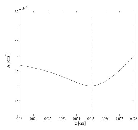
Figure 1: Dependence of the cross section of the de Laval nozzle on the position $z$ for a velocity field given by Eq. (6) and depicted in Fig. 2. The vertical dashed line corresponds to the location of the sonic horizon $z_{H}=0.025$ cm.

where $z=z_{H}$ denotes the position of the waist of the nozzle (the sonic horizon). In the laboratory frame the fluid is moving from right to left, so $v<0$ and the sonic horizon occurs where $v=-c$. The constant $D$ entering the continuity equation is determined by requiring the fluid to be sonic at the waist; i.e.,

$$D=-cA_{H}\rho_{0}e^{-1/2}=-\frac{A_{H}p_{H}}{c}\ ,$$ (7)

where $A_{H}$ is the area at the horizon, $p_{H}$ the pressure and $\rho_{0}=p_{H}e^{1/2}/c^{2}$. Given this, the profile of the nozzle can be computed from Eq. (1) and is depicted in Fig. 1, where we have used $A_{H}=10^{-8}$ cm², $\beta=600$ cm^-1, $p_{H}=2\times 10^{6}$ Pa and $c=250$ m/s. These latter two are typical values for liquid Helium. The profiles of density and velocity are shown in Fig. 2, where the significant range of $z$ is $[0,0.05]$ cm; the horizon lies at $z_{H}=0.025$ cm and its location is indicated by a vertical dashed line in the figures. In the region $z>z_{H}$ the motion of the fluid is subsonic; the acoustic black hole is the region $z<z_{H}$.

As shown by Unruh unruh81 , sound waves propagating in an inhomogeneous fluid are described as a massless scalar field propagating in an effective curved spacetime described by an “acoustic metric” which depends on $\rho$ and $v$. Quantization of these modes leads to the conclusion that in presence of a sonic horizon a thermal emission of phonons is expected, in complete analogy of what Hawking found for gravitational black holes. The emission temperature of the phonons is $T_{H}=\hbar k/(2\pi c\kappa_{B})$, where $k$ is the surface gravity of the sonic horizon, defined as

$$k=\left.\frac{1}{2}\frac{d}{dn}(c^{2}-v^{2})\right|_{z_{H}}\ .$$ (8)

$\kappa_{B}$ is the Boltzmann constant and $n$ is the normal to the horizon.

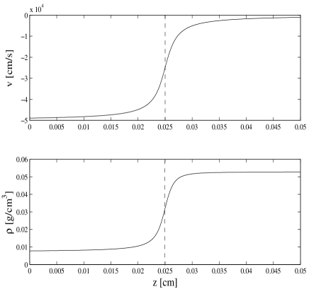
Figure 2: Velocity (top) and density (bottom) from Eq. (6). The vertical dashed line correspond to the location of the sonic horizon ($z_{H}=0.025$ cm). The sonic black hole corresponds to $z<z_{H}$.

For the specific acoustic black hole model we consider in this paper, $T_{H}=1.1598\times 10^{-5}$ ^∘K.

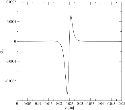
Figure 3: Quantum sources in the Unruh state (solid lines) and in the Hartle-Hawking state (dashed line). To appreciate the difference in $F_{2}$ taken in the Hartle-Hawking and Unruh states, we show it in the inset. The $G_{2}$ is the same for both states. The sonic horizon is located at $z_{H}=0.025$ cm.

III The backrection equations

The phonons quantum emission previously discussed modifies the underlying fluid flow according to the backreaction equations derived in Ref. nostri , to which we refer for further details. For a one-dimensional flow, they read

$$A\rho_{B}+\partial_{z}(A\rho_{B}v_{B}) =\partial_{z}\left[\frac{1}{c}(\langle T_{tz}^{(2)}\rangle+v\langle T_{zz}^{(2)}\rangle)\right]\ ,$$ (9)

$$A\left[\dot{\psi}_{B}+\frac{v_{B}^{2}}{2}+\mu(\rho_{B})\right] =\frac{1}{2}\langle T^{(2)}\rangle\ .$$ (10)

Here $\rho_{B}$ and $v_{B}$ are the quantum corrected density and velocity fields and $\psi_{B}$ is the velocity potential; i.e., $\partial_{z}\psi_{B}=v_{B}$; the overdot stands for time derivative. The $\langle T_{ab}^{(2)}\rangle$ which drive the backreaction are the quantum expectation values of the pseudo energy momentum tensor quadratic in the phonons field. To evaluate $(\rho_{B},v_{B})$ up to $O(\hbar)$ terms, the r.h.s. of the backreaction equations (9) and (10) needs just to be evaluated on the classical background $(\rho,v)$ of Sec. II.

The quantum state of the field in which the expectation values have to be computed depends on the physical situation one wants to describe. For an isolated hole, the escaping phonons radiation leads to a time variation of the underlying medium, i.e. $\rho_{B}(t,z)$ and $v_{B}(t,z)$. The appropriate quantum state in this case is the analogue of the Unruh state unruh76 . In case the system is maintained in thermal equilibrium with the surroundings (that is, putting a sonic cavity in the subsonic asymptotic right region), the quantum state is the analogue of the Hartle-Hawking state HH , the thermal equilibrium state at $T=T_{H}$. In this case the system remains stationary, i.e. $\rho_{B}(z)$ and $v_{B}(z)$.

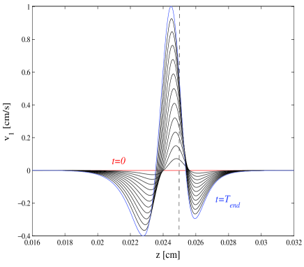
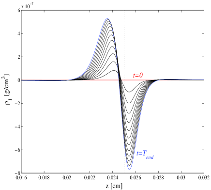
Figure 4: Unruh state: time evolution of the backreaction equations for $c\kappa t\ll 1$. Snapshots of the quantum correction to the velocity $v_{1}$ (left panel) and to the density (right panel) for an evolution time $t_{\rm end}=0.2\,t_{\rm max}\approx 2.09\times 10^{-2}$ $\mu$s ($c\kappa t=0.2$). The vertical dashed line corresponds to the location of the classical sonic horizon. The delay between one snapshot and the other (between $t=0$ and $t=t_{\rm end}$) is $\Delta t\approx 1.74\times 10^{-3}$ $\mu$s.

Neglecting backscattering of the phonons, $\langle T_{ab}^{(2)}\rangle$ can be approximated with the Polyakov stress tensor polyakov ; sandro-pepe . Introducing for the sake of simplicity null coordinates

$$x_{\pm}=c\left(t\mp\int\frac{dz}{c\pm v}\right)\,$$ (11)

the Polyakov stress tensor reads:

$$\langle T_{\pm\pm}^{(2)}\rangle = -\frac{\hbar}{12\pi}C^{1/2}C^{-1/2}_{,\pm\pm}+\Delta_{\pm\pm}$$ (12)

$$\langle T^{(2)}\rangle = \frac{\hbar}{6\pi}C^{-1}\left(\ln C\right)_{,+-}\ ,$$ (13)

where

$$C=\frac{\rho}{c}\frac{c^{2}-v^{2}}{c^{2}}$$ (14)

and $\Delta_{\pm\pm}$ are functions which depend on the choice of the quantum state of the phonons field. For the Unruh state:

$$\Delta_{++}\equiv\Delta^{\rm U}_{++} = 0\ ,$$ (15)

$$\Delta_{--}\equiv\Delta^{\rm U}_{--} = \frac{\hbar k^{2}}{48\pi c^{4}}\ .$$ (16)

For the Hartle-Hawking state instead

$$\Delta_{\pm\pm}\equiv\Delta^{\rm HH}_{\pm\pm}=\frac{\hbar k^{2}}{48\pi c^{4}}\ .$$ (17)

From Eqs. (15)–(17) it follows that, in the asymptotic subsonic region $z\rightarrow+\infty$, $\Delta^{\rm U}_{\pm\pm}$ describes a flux of phonons at a temperature $T_{H}$, whereas $\Delta^{\rm HH}_{\pm\pm}$ describes a two-dimensional gas of phonons at thermal equilibrium at the temperature $T_{H}$. To find first order in $\hbar$ corrections to the classical sonic black hole fluid configuration $(\rho(z),v(z))$ described in Eqs. (5) and (6) we write

$$\psi_{B} = \psi(z)+\epsilon\psi_{1}(t,z)\ ,$$ (18)

$$\rho_{B} = \rho(z)+\epsilon\rho_{1}(t,z)\ ,$$ (19)

with $v_{B}=\partial_{z}\psi_{B}$ and $\epsilon$ is a dimensionless expansion parameter york :

$$\epsilon=\frac{\hbar}{|D|A_{H}}\ .$$ (20)

For our system $\epsilon=1.317\times 10^{-14}$.
The backreaction equations linearized in $\epsilon$ then become

$$\epsilon\bigg{\{}A\dot{\rho}_{1}+\partial_{z}\left[A(\rho_{1}v+\rho v_{1})\right]\bigg{\}}$$

$$\qquad\qquad=c^{2}\partial_{z}\left[\dfrac{\langle T_{++}^{(2)}\rangle}{(c-v)^{2}}-\dfrac{\langle T_{--}^{(2)}\rangle}{(c+v)^{2}}\right]\equiv\epsilon F_{2}\ ,$$ (21)

$$\epsilon\left[A\left(\dot{\psi}_{1}+vv_{1}+\frac{c^{2}}{\rho}\rho_{1}\right)\right]=\frac{\langle T^{(2)}\rangle}{2}\equiv\epsilon G_{2}\ .$$ (22)

Using the background equations (1) and (2), satisfied by $\rho$ and $v$, the continuity equation can be rewritten as

$$\dot{\rho_{1}}+v\rho_{1}^{\prime}+\frac{v^{2}v^{\prime}}{c^{2}}\rho_{1}-\dfrac{\rho v^{\prime}}{v}\psi_{1}^{\prime}+\rho\psi_{1}^{\prime\prime}=\frac{F_{2}}{A}\ ,$$ (23)

whereas the Bernoulli equation is

$$\dot{\psi_{1}}+v\psi_{1}^{\prime}+\frac{c^{2}}{\rho}\rho_{1}=\frac{G_{2}}{A}\ ,$$ (24)

with a prime indicating derivative with respect to $z$.

The profiles for the quantum sources $F_{2}$ and $G_{2}$ are depicted in Fig. 3 for the Unruh state (solid line) and for the Hartle-Hawking state (dashed line). The difference between the states is reflected on $F_{2}$ only (and is shown in the inset in the left panel of the figure), while $G_{2}$, being related to the trace anomaly which is state-independent, is unchanged. One can note the appearance of a maximum and a minimum in the region $z\in[0.02,0.03]$ cm. Outside this range, $F_{2}$ and $G_{2}$ rapidly drop to zero. The analysis of Ref. nostri , being limited to the region very near to $z_{H}$, could not catch this non trivial structure.

IV Unruh state

As said before, in Ref. nostri the backreaction equations were analytically solved just for $z\approx z_{H}$ to allow a Taylor expansion of the sources up to linear terms. In this section we compute the numerical solution all over the nozzle. We finite-difference the system of Eqs. (23) and (24) and solve it numerically in the time domain as an initial value problem. The equations are discretized on an evenly spaced grid $(0,z_{\rm c})$ with $z_{\rm c}=0.05$ cm. Following a standard convention in numerical fluid mechanics leveque , we have used a staggered grid, i.e. both $z=0$ and $z=z_{\rm c}$ are thought to lie on cell interfaces while the hydrodynamics quantities are defined on cell centers. As a result, the first point of our computational domain is $z_{1}=\Delta z/2$ and the last is $z_{i_{\rm max}}=z_{\rm c}-\Delta z/2$. We notice that $\Delta z$ is chosen so that the horizon is located at a cell interface. The reason for this is that, even though the square bracket on the r.h.s. of Eq. (21) is analytically regular at $z=z_{H}$ (where $v=-c$), the presence of the combination ($c+v$) at denominator in Eq. (23) can give problems (i.e., division by zero) due to the discretization procedure. The use of a staggered grid bypasses this difficulty since the sonic point turns out to be always displaced with respect to the grid points.

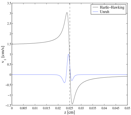
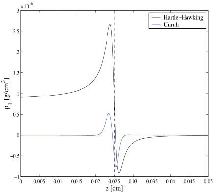
Figure 5: Profile of the quantum correction to the velocity $v_{1}$ (left panel) and to $\rho_{1}$ (right panel) due to backreaction in the Hartle-Hawking state (black lines), compared with the profile of $v_{1}$ and $\rho_{1}$ at $t=t_{\rm end}$ in the Unruh state (blue lines). The vertical dashed lines correspond to the position of the sonic horizon at $t=0$.

Initial conditions are chosen so that at $t=0$ the solution is the classical one; i.e., $\rho_{1}(t=0)=\psi_{1}(t=0)=0$. Then the backreaction is switched on. As in Ref. nostri , since the quantum sources are computed only for the static classical background, the validity of the solution is limited by the condition $c\kappa t\ll 1$, where we have introduced the constant $\kappa$ as

$$\kappa=c^{-2}k=c^{-1}\left.\frac{dv}{dz}\right|_{z_{H}}$$ (25)

with dimension $[\rm length]^{-1}$. For the sonic black hole considered here, the short time condition determines a maximum evolution time ($c\kappa t=1$) of $t_{\rm max}=0.104\ \mu s$; so it is possible to extract only informations about how the backreaction starts.

Before discussing our numerical results, we briefly describe the numerical algorithms implemented, further details can be found in Appendix A.

We are dealing with a system of Partial Differential Equations (PDEs), where the equation for $\rho_{1}$ is of convection-diffusion type, due to the parabolic term proportional to $\psi_{1}^{\prime\prime}$, while the equation for $\psi_{1}$ is a simple hyperbolic advection equation. As a result, the numerical algorithm must be designed accordingly gustaf . For the equation for $\psi_{1}$ a simple first-order upwind method is well suited to solve it; for the parabolic equation we have implemented standard Forward-Time-Centered-Space (FTCS) explicit method, as well as standard Backward-Time-Centered-Space (BTCS) implicit method. Due to the short evolution time needed, the limitation of the time–step required by the FTCS and the consequent high number of iterations is not a drawback; in any case, we tested one method versus the other and we obtained equivalent results. In fact, to have a stable evolution, the time step is selected according to the condition $\Delta t=\alpha\Delta z^{2}/\mbox{max}(\rho)$, since $\rho$ is the coefficient of the $\psi_{1}^{\prime\prime}$ term in the equation for $\rho_{1}$. In addition, for the nozzle considered, we have checked that a resolution of $\Delta z=2.5\times 10^{-5}$ cm (which corresponds to $2000$ points covering the numerical domain) is sufficient to be in the convergence regime (see Appendix A for discussion).

In Fig. 4 we have snapshots of the time evolution of the profiles of $v_{1}$ (left panel) and $\rho_{1}$ (right panel). For this particular computation, we have considered a total evolution time $t_{\rm end}=0.2\ t_{\rm max}$. The initial and final snapshots are depicted in red and blue respectively. The time delay between one snapshot and the other is $\Delta t\simeq 1.74\times 10^{-3}\mu$s. The quantum corrected velocity is obtained as $v_{1}=\partial_{z}\psi_{1}$, the derivative being computed directly from the numerical data by means of a second order finite-difference approximation.

The numerical solution confirms the near horizon behaviour obtained in Ref. nostri : the fluid slows down close to the horizon ($v_{1}>0$, remember that $v<0$ because the fluid flows from right to left), causing the horizon to move to the left, and the total density decreases ($\rho_{1}<0$). In addition, now (even if for small times) it is possible to see the influence of the quantum corrections all over the sonic hole, and not just in the neighborhood of the horizon. As a consequence of the shape of the quantum sources $F_{2}$ and $G_{2}$ (see Fig. 3) the complex structure of Fig. 4 emerges. One can see that in the region near the horizon the fluid slows down, but there are also regions where the phonons emission induces acceleration.

V Hartle-Hawking state

The thermal equilibrium configuration of the Hartle-Hawking state is much simpler to treat. Since the time dependence drops off, the backreaction equations (23) and (24) become a simple system of algebraic equations relating $\rho_{1}$ and $v_{1}$:

$$A\left(\rho_{1}v+\rho v_{1}\right) =\int_{z_{H}}^{z}d\xi F_{2}(\xi)+\mbox{const}\ ,$$ (26)

$$A\left(vv_{1}+\frac{c^{2}}{\rho\texttimes}\rho_{1}\right) =G_{2}\ .$$ (27)

The integration constant in Eq. (26) is chosen to be zero in order to make the solution non singular on the horizon.

The profile for $v_{1}$ and $\rho_{1}$ are depicted in Fig. 5 (black line); for the sake of comparison, we show in the same plot the profile of $v_{1}$ and $\rho_{1}$ in the Unruh state for $t=t_{\rm end}$ (blue line). In both cases the quantum backreaction correction to the velocity is positive at $z=z_{H}$ (vertical dashed line).

In the region very close to the horizon one can make as in Ref. nostri a Taylor expansion for the background up to order $O((z-z_{H})^{5})$. This allows the source terms to be evaluated up to linear term

$$F_{2} = \frac{|D|A_{H}\kappa^{3}}{96\pi}\bigg{[}-(\pi^{2}+10)$$

$$- \dfrac{\pi^{4}+25\pi^{2}-24}{2}\kappa(z-z_{H})+O(\kappa^{2}(z-z_{H})^{2})\bigg{]}\ ,$$

$$G_{2} = \frac{A_{H}^{2}c^{2}\kappa^{2}}{48\pi}$$ (29)

$$\times \left[(\pi^{2}+6)\kappa(z-z_{H})+O(\kappa^{2}(z-z_{H})^{2})\right]\ .$$

The corresponding quantum corrections to the velocity and to the density are

$$v_{1} =\frac{A_{H}c\kappa^{2}}{192\pi}\bigg{[}2+\pi^{2}$$

$$-\dfrac{52+35\pi^{2}+\pi^{4}}{4}\kappa(z-z_{H})+O(\kappa^{2}(z-z_{H})^{2})\bigg{]}\ ,$$ (30)

$$\rho_{1} =\frac{|D|\kappa^{2}}{192c\pi}\bigg{[}2+\pi^{2}$$

$$+\dfrac{44-19\pi^{2}-\pi^{4}}{4}\kappa(z-z_{H})+O(\kappa^{2}(z-z_{H})^{2})\bigg{]}\ .$$ (31)

Setting $v_{B}=v+\epsilon v_{1}=-c$ one finds the quantum corrected position of the horizon $z_{H}^{q}$

$$z_{H}^{q}=z_{H}-\frac{\pi^{2}+2}{192\pi}\,\epsilon A_{H}\kappa\ ,$$ (32)

which is shifted to the left of $z_{H}$.
The quantum corrected equilibrium temperature can also be simply obtained by evaluating Eq. (8) at $z=z_{H}^{q}$ with $v$ replaced by $v_{B}$. The result is

$$T_{H}^{q}=\frac{\hbar c\kappa}{2\pi\kappa_{B}}\bigg{[}1-\dfrac{\epsilon A_{H}}{768\pi}\left(52+35\pi^{2}+\pi^{4}\right)\kappa^{2}\bigg{]}\ ,$$ (33)

which indicates that, taking into account the backreaction, the equilibrium temperature is lowered.

VI Conclusions

Using the continuity and Bernoulli equations, the quantum correction (first order in $\hbar$) to a classical stationary flow describing an acoustic black hole has been evaluated in a one-dimensional approximation.
The quantum corrections to the velocity $v_{1}$ and to the density $\rho_{1}$ profiles for the equilibrium configuration (Hartle-Hawking state) are depicted in Fig. 5 (black lines). The phonons backreaction causes the fluid to slow down in the supersonic region, with the consequence of a shift of the horizon to the left of the waist of the nozzle (see Eq. (32)). In the subsonic region the velocity increases, but the magnitude of the change is smaller than the previous one. One finds a similar shape for the density correction $\rho_{1}$, which increases in the supersonic region and slightly decreases in the subsonic one. Finally the equilibrium temperature appears to have been lowered by the backreaction from its zero-order value $\hbar c\kappa/2\pi\kappa_{B}$ (see Eq. (33)).

For the time-dependent case (Unruh state) the analysis has been restricted to very short times after switching on the phonons radiation. This because the quantum source ($F_{2}$ and $G_{2}$ in Eqs. (21)-(22)) has been computed only for the classical background, which just represents the initial configuration of the acoustic black hole. A more rigorous analysis requires the time-dependence of the sources to be included.

Within these limitations, one sees (Fig. 4) a deceleration of the fluid in the supersonic region, which causes a drift of the horizon towards the left of the nozzle. Two acceleration regions also appear on both sides of the horizon, but the intensity of the effect is lower. On the other hand, the density correction $\rho_{1}$ reflects the behaviour it shows in the Hartle-Hawking state (on a reduced scale).

Appendix A Numerical schemes

In this section we report explicitly the time-evolution algorithms. In the main text, we said that we used a standard upwind method for the equation for $\psi_{1}$ and standard explicit Forward-Time-Centered-Space (FTCS) or an implicit Backward-Time-Centered-Space (BTCS) schemes for that for $\rho_{1}$. In practice the upwind method reads leveque

$$\psi_{1,i}^{n+1} =\psi_{1,i}^{n}-v_{i}\frac{\Delta t}{\Delta z}\left(\psi_{1,i+1}^{n}-\psi_{1,i}^{n}\right)$$

$$\qquad\quad+\Delta t\left(-\frac{c^{2}}{\rho_{i}}\rho_{1,i}^{n}+G_{2,i}A_{i}^{-1}\right)\ .$$ (34)

The FTCS (explicit) and the BTCS (implicit) schemes for the equation for $\rho_{1}$ respectively read

$$\rho_{1,i}^{n+1} =\rho_{1,i}^{n}-\frac{v_{i}\Delta t}{2\Delta z}\left(\rho_{1,i+1}^{n}-\rho_{1,i-1}^{n}\right)+\frac{\rho_{i}^{n}v^{\prime}_{i}}{v_{i}}\frac{\Delta t}{2\Delta z}\left(\psi_{1,i+1}^{n}-\psi_{1,i-1}^{n}\right)-\rho_{i}^{n}\frac{\Delta t}{\Delta z^{2}}\left(\psi^{n}_{1,i+1}-2\psi^{n}_{1,i}+\psi^{n}_{1,i-1}\right)$$

$$+\Delta t\left(-\frac{v_{i}^{2}v_{i}^{\prime}}{c^{2}}\rho_{1,i}^{n}+F_{2,i}A_{i}^{-1}\right)\ ,$$ (35)

$$-\frac{v_{i}\Delta t}{2\Delta z}\rho_{1,i-1}^{n+1} +\left(1+\frac{v^{2}_{i}v^{\prime}_{i}}{c^{2}}\Delta t\right)\rho_{1,i}^{n+1}+\frac{v_{i}\Delta t}{2\Delta z}\rho_{1,i+1}^{n+1}=\rho_{1,i}^{n}+\Delta t\bigg{\{}F_{2,i}A^{-1}_{i}+\dfrac{\rho_{i}^{n}v^{\prime}_{i}}{v_{i}}\frac{\psi^{n+1}_{1,i+1}-\psi^{n+1}_{1,i-1}}{2\Delta z}$$

$$-\rho_{i}^{n}\frac{\psi_{1,i+1}^{n+1}-2\psi_{1,i}^{n+1}+\psi_{1,i-1}^{n+1}}{\Delta z^{2}}\bigg{\}}\ .$$ (36)

where the cell index $i$ runs from one to $i_{\rm max}$. In the case of the BTCS scheme $\rho_{1}$ is obtained at every time slice (labelled by index $n$) as the solution of a tridiagonal linear system of the form $a_{i}u_{i-1}^{n}+b_{i}u_{i}^{n}+c_{i}u_{i+1}^{n}=f_{i}^{n}$ that can be accomplished by a standard lower-upper ($LU$) decomposition of the matrix to be inverted NR . A careful treatment of the boundaries $z=0$ and $z=z_{\rm c}$ of the numerical domain is crucial for selecting the correct solution, especially when the implicit method is employed and so the inversion of the associated coefficient matrix is concerned. According to the physical meaning of the Unruh state, we impose outgoing conditions at both boundaries, i.e. $u_{i-1}^{n}=u_{i}^{n}$ at $i=1$ and $u_{i+1}^{n}=u_{i}^{n}$ at $i=i_{\rm max}$ where $u^{n}$ can be either $\rho_{1}$ or $\psi_{1}$. If $\rho_{1}$ is solved using the FTCS scheme, since the method is explicit and no matrix inversion is needed, the problem of setting correct boundary conditions is less important; in fact, it is enough to put the boundaries far enough from $z_{H}$ to avoid any influence on the evolution. For this kind of equations, stability has also proved to be an issue. Implementing the FTCS scheme, to have a stable evolution the time step is selected according to the condition $\Delta t=\alpha\Delta z^{2}/{\rm max}(\rho)$. For the nozzle model discussed in this paper, we have used $\alpha=1\times 10^{-4}$ to avoid stability problems and the same choice was kept also for the BTCS scheme, which results in roughly $3\times 10^{4}$ integration steps. This is not particularly expensive from the computational point of view. For example, for the results presented here we used a resolution of $\Delta z=2.5\times 10^{-5}$ cm (corresponding to $2000$ grid points) and the total evolution took $\sim 11$s time evolution on a single-processor machine with a Pentium^TM M processor at 1.3GHz. The code was compiled using an Intel^TM Fortran Compiler.

We checked convergence of the numerical method (using both BTCS or FTCS schemes) using resolutions of 500, 1000, 2000 and 4000 points, considering the case of 8000 points as reference. We computed the error $\Delta f$ with respect to the reference resolution as a root mean square for $f=\psi_{1}$ and $f=\rho_{1}$. From the relation $\Delta f={\cal K}\Delta z^{\sigma}$ we evaluated the convergence rate $\sigma$ and we obtained $\sigma\approx 1.3$ for both $\psi_{1}$ and $\rho_{1}$. We have verified that $2000\div 4000$ grid points are sufficient to be in the convergence regime.

References

- (1) S.W. Hawking, Nature 248, 30 (1974)
- (2) W.G. Unruh, Phys. Rev. Lett. 46, 1351 (1981)
- (3) R. Courant and K.O. Friedrichs Supersonic flows and shock waves, Springer-Verlag (1948)
- (4) Artificial black holes, eds. M. Novello, M. Visser and G.E. Volovik, World Scientific, River Edge, USA (2002)
- (5) C. Barcelò, S. Liberati and M. Visser, Analogue Gravity, gr-qc/0505065 (2005)
- (6) R. Balbinot, S. Fagnocchi, A. Fabbri and G.P. Procopio, Phys. Rev. Lett. 94, 161302 (2005); R. Balbinot, S. Fagnocchi and A. Fabbri, Phys. Rev. D71, 064019 (2005)
- (7) W.G. Unruh, Phys. Rev. D14, 870 (1976)
- (8) J.B. Hartle and S.W. Hawking, Phys. Rev. D13, 2188 (1976)
- (9) A.M. Polyakov, Phys. Lett. 103 B, 207 (1981)
- (10) A. Fabbri and J. Navarro-Salas, Modeling black hole evaporation, Imperial College Press, London (2005).
- (11) For a gravitational black hole the analogous expansion parameter is given by the square of the ratio between the Planck length and the horizon size, i.e. in units , see J.W. York, Phys. Rev. D31, 775 (1985)
- (12) B. Gustafsson, H.O. Kreiss and J. Oliger, Time dependent problems and difference methods, John Wiley and Sons, Inc. (1995)
- (13) R.J. Le Veque, Numerical Methods for Conservations Laws, Birkhäuser Verlag (1992)
- (14) W.H. Press, S.A. Teukolsky, W.T. Vetterling and B.P. Flannery, Numerical Recipes, The Art of Scientific Computing, Cambridge University Press (1992)