Constant scalar curvature hypersurfaces in extended Schwarzschild space-time

Abstract.

We present a class of spherically symmetric hypersurfaces in the Kruskal extension of the Schwarzschild space-time. The hypersurfaces have constant negative scalar curvature, so they are hyperboloidal in the regions of space-time which are asymptotically flat.

1. Introduction

Hyperboloidal hypersurfaces have gained some importance in the study of radiative systems in General Relativity. This is because in a sense they interpolate between space-like hypersurfaces which become asymptotically flat and null hypersurfaces which extend out to null-infinity. Since these hypersurfaces are space-like one can use them to formulate an initial-value formulation for the Einstein equations and because they extend to null-infinity one has in principle full control over the radiation which propagates outward. One can even go further and compactify the space-time following the work of Penrose [1] and arrive at the system of conformal field equations set up by Friedrich [2, 3]. For a review on these matters see [4].

In the asymptotically flat regions of a space-time hyperboloidal hypersurfaces behave like the space-like hyperboloids in Minkowski space-time. These are defined by $t^{2}-r^{2}=\mathrm{const}\equiv A^{-2}$. They are the only everywhere smooth spherically symmetric hypersurfaces with constant mean curvature in Minkowski space-time. They also have constant negative curvature $\mathcal{R}=-6A^{2}$. When studying the properties of hyperboloidal hypersurfaces in simple examples like the Schwarzschild and Kruskal space-times we noticed that much is known for hypersurfaces with constant mean curvature (see [5, 6] and references therein), while the class of hypersurfaces with constant scalar curvature (CSC) seems to have been ignored. Therefore, we decided to explore this class of hypersurfaces in some detail.

We find that hypersurfaces in this class are characterised by three constants: the scalar curvature, the location of the hypersurface in space-time (i.e. an event in space-time lying on the hypersurface), and an integration constant. The hypersurfaces can be space-like or time-like. The latter ones either connect the white-hole singularity with the black-hole singularity or they ’stop’ with a diverging extrinsic curvature somewhere inside the white-hole. Most space-like hypersurfaces connect one asymptotic region of the Kruskal extension with the other one. But they all remain below the bifurcation sphere. There is another class of space-like hypersurfaces which come in from null-infinity and reach a minimal radius where the extrinsic curvature diverges.

The paper is organised as follows. In sect. 2 we solve the constraints for a hypersurface with constant negative scalar curvature. In sect. 3 we discuss the embedding equation for such hypersurfaces in Schwarzschild and derive the qualitative behaviour of the embedded slices. In sect. 4 we look at the behaviour of the hypersurfaces in the Kruskal extension of the Schwarzschild space-time and close the paper with a short discussion of our findings.

2. Initial data sets with constant scalar curvature

In this first section we want to determine spherically symmetric initial data $(g_{ab},K_{ab})$ on a 3-dimensional hypersurface $\Sigma$ with constant scalar curvature. In our discussion we follow closely the treatment of [6]. First we determine the spherically symmetric metrics with constant scalar curvature and then proceed to solve the vacuum constraints for the extrinsic curvature.

2.1. 3-metrics with constant scalar curvature

We are interested in spherically symmetric 3-dimensional metrics with constant negative scalar curvature $\mathcal{R}$ on a 3-manifold $\Sigma$. These can be obtained directly by solving the equation

$$\mathcal{R}=-6A^{2}=const\,,$$

where $A$ is an arbitrary positive constant on $\Sigma$. The general spherically symmetric metric on a 3-dimensional manifold can be written in the form

$$g=\mathrm{d}s^{2}+f(s)^{2}\,\mathrm{d}\sigma^{2}\,,$$

where $s$ is the geodesic radial distance on the 3-manifold and $\mathrm{d}\sigma^{2}$ is the metric on the unit 2-sphere. The function $f$ determines the radius $r$ of the spheres of symmetry and hence determines the intrinsic geometry. We find the scalar curvature for this metric and obtain the equation

$$\mathcal{R}=-6A^{2}=-4\frac{f^{\prime\prime}}{f}-\frac{2f^{\prime 2}}{f^{2}}+\frac{2}{f^{2}}\,.$$

Multiplying with $f^{\prime}$ and rearranging we obtain the equation

$$(1+3A^{2}f^{2})f^{\prime}=2ff^{\prime}f^{\prime\prime}+f^{\prime 3}=(ff^{\prime 2})^{\prime}\,,$$

which can be integrated once

$$f+A^{2}f^{3}=ff^{\prime 2}+2C$$

with an integration constant $C$. Then we can write

$$f^{\prime 2}=1-\frac{2C}{f}+A^{2}f^{2}$$

and this equation cannot be integrated in closed form any further. The explicit solution involves elliptic integrals and is not very illuminating. However, writing $r=f(s)$ and introducing $r$ as a new coordinate, the metric takes the form

(1) $$g=\frac{\mathrm{d}r^{2}}{1-\frac{2C}{r}+A^{2}r^{2}}+r^{2}\mathrm{d}\sigma^{2}\,.$$

Clearly, rescaling the metric with a constant $\lambda$ so that $g\mapsto\lambda^{2}g$ rescales the scalar curvature $\mathcal{R}\mapsto\mathcal{R}/\lambda^{2}$ so that $A\mapsto A/\lambda$. This can also be seen from (1) which, in addition, reveals that $C\mapsto\lambda C$. Note that the transition to this form (1) of the metric is valid only as long as $f^{\prime}(s)\neq 0$.

2.2. Solving the constraints

We consider now the vacuum constraints. They are written as

$$\mathcal{R}-K_{a}{}^{b}K_{b}{}^{a}+(\mathrm{tr}K)^{2}=0\,,$$

$$\partial_{a}K_{b}{}^{a}-\partial_{b}\mathrm{tr}K=0\,.$$

Here $\partial_{a}$ denotes the covariant derivative compatible with the metric $g_{ab}$ and $\mathrm{trK}=K_{c}{}^{c}$. Using the spherical symmetry we find that the extrinsic curvature necessarily has the form

$$K_{ab}\,\mathrm{d}x^{a}\mathrm{d}x^{b}=\tilde{k}(r)\,\mathrm{d}r^{2}+\tilde{\kappa}(r)\,\mathrm{d}\sigma^{2}\,,$$

for two functions $\tilde{k}(r)$ and $\tilde{\kappa}(r)$. Therefore, the $(1,1)$-tensor $K_{a}{}^{b}$ is diagonal in the given coordinate basis with components

(2) $$K_{a}{}^{b}\doteq\mathrm{diag}(k(r),\kappa(r),\kappa(r))\,.$$

Hence, the trace of the extrinsic curvature is

$$\mathrm{tr}K=k+2\kappa=:3K\,,$$

thus defining the mean curvature $K(r)$. Expressing $\kappa$ in terms of $K$ and $k$ as

$$\kappa(r)=\frac{1}{2}\left(3K(r)-k(r)\right)$$

and inserting into the constraints we have

(3) $$\mathcal{R}-\left(k^{2}+\frac{1}{2}\left(3K-k\right)^{2}\right)+9K^{2}=0\,,$$

(4) $$r\partial_{r}(k-3K)=-3(k-K)\,.$$

Here the metric has a constant negative scalar curvature $\mathcal{R}$, which we write as $\mathcal{R}=-6A^{2}$ as before. Rescaling the metric with a constant $\lambda^{2}$ results by virtue of the constraint equations in a rescaling of the extrinsic curvature $K_{ab}$ with $\lambda$. In other words, when $(g_{ab},K_{ab})$ is a solution of the constraints, then $(\lambda^{2}g_{ab},\lambda K_{ab})$ is also a solution.

We first solve the Hamiltonian constraint for the function $k$

(5) $$k=K\pm 2\sqrt{K^{2}-A^{2}}$$

and insert this into the momentum constraint. We get the equation

(6) $$A^{2}rK^{\prime}=-3(K^{2}-A^{2})\left(K\pm\sqrt{K^{2}-A^{2}}\right)\,.$$

This equation has the solution

(7) $$K(r)=\mp A\frac{r^{3}+D^{3}}{\sqrt{r^{3}(r^{3}+2D^{3})}}\,,$$

for some constant of integration $D$. For $D>0$ the mean curvature is defined for all values of $r$, while for $D<0$ there is only a limited range given by $r>-2^{1/3}D$. This means that the hypersurface has to stop somewhere because the extrinsic curvature blows up. For $D=0$ we have constant mean curvature. From (5) we find

(8) $$k(r)=\mp A\frac{r^{3}-D^{3}}{\sqrt{r^{3}(r^{3}+2D^{3})}}$$

and, finally,

(9) $$\kappa(r)=\mp A\sqrt{1+2(D/r)^{3}}\,.$$

The ambiguity in sign is inherent in the vacuum constraints because with $K_{ab}$ also $-K_{ab}$ is a solution of the constraints. It corresponds to the choice of the time orientation. We will concentrate in the following on the $+$ sign, the case where the mean curvature is positive. Then $K(r)>A$ and approaches $A$ for $r\to\infty$.

So far we have not considered the fact that the hypersurface should be embedded in the Schwarzschild space-time. This can be taken into account by the consideration of the Misner-Sharp mass [7]. This mass $m(r,t)$ is defined in a spherically symmetric space-time by the equation

$$g_{rr}=\left(1-\frac{2m(r,t)}{r}+U(r,t)^{2}\right)^{-1},$$

where, in our case, $U(r,t)=r\kappa(r)$, and it has the property that in the Schwarzschild space-time it is constant, equal to the mass parameter $m$. Inserting $g_{rr}$ from (1) and $\kappa(r)$ from above we obtain a relation between the integration constants $D$, $C$, and $A$

(10) $$m-C=A^{2}D^{3}.$$

In particular, substituting into (7), the mean curvature in terms of $m$ and $C$ is

(11) $$K(r)=\frac{A^{2}r^{3}+m-C}{\sqrt{r^{3}(A^{2}r^{3}+2(m-C))}}\,.$$

Remarkably, the case $C=m$, in which $K(r)=A$ and also $k(r)=\kappa(r)=A$, characterises a hypersurface with constant mean curvature and constant scalar curvature, for which the extrinsic curvature is ‘pure trace’ $K_{ab}=A\,g_{ab}$.

3. Embedding CSC slices in Schwarzschild space-time

In the next two sections we ask how hypersurfaces with the intrinsic and extrinsic geometries determined in the previous sections can be embedded into the Schwarzschild space-time. We first discuss this question in the well-known chart of Schwarzschild coordinates and discuss the qualitative behaviour of the hypersurfaces. Then we write down a system of equations for use in the Kruskal completion of the Schwarzschild space-time.

3.1. Schwarzschild coordinates

We consider the Schwarzschild space-time and write its metric in the usual Schwarzschild coordinates $t$ and $r$. However, in order to simplify the formulae we rescale the coordinates with $2m$, i.e. we measure them in units of the Schwarzschild radius. Then the areal radius is $2mr$. In these coordinates the metric is

$$\mathrm{d}s^{2}=4m^{2}\left\{-\left(1-\frac{1}{r}\right)\mathrm{d}t^{2}+\left(1-\frac{1}{r}\right)^{-1}\mathrm{d}r^{2}+r^{2}\mathrm{d}\sigma^{2}\right\}\,,$$

which is valid for $0<r<1$ or $r>1$. We locate a spherically symmetric hypersurface by using a height-function $h$ with an equation of the form

$$t=h(r)\,.$$

For such a hypersurface one can find the intrinsic metric, the normal vector, and the extrinsic curvature expressed in terms of derivatives of the height function. The intrinsic metric is

(12) $$g=4m^{2}\left\{F\,\mathrm{d}r^{2}+r^{2}\mathrm{d}\sigma^{2}\right\}\,,$$

with

$$F=\frac{r}{r-1}-\frac{r-1}{r}\,h^{\prime}(r)^{2}\,.$$

Notice, the hypersurface will be space-like (resp. time-like, null) whenever $F>0$ ($F<0$, $F=0$). Defining $N=1/\sqrt{|F|}$, the normal unit vector is

(13) $$n=\frac{N}{2m}\left(\frac{r}{r-1}\,\partial_{t}+h^{\prime}\frac{r-1}{r}\,\partial_{r}\right)\,.$$

This vector is chosen such that it is future-pointing whenever $F>0$. From this expression we compute the extrinsic curvature

(14) $$K_{ab}\,\mathrm{d}x^{a}\mathrm{d}x^{b}=\frac{2m}{N^{2}}\left(Nh^{\prime}\left(1-\frac{1}{r}\right)\right)^{\prime}\,\mathrm{d}r^{2}+2mr\left(Nh^{\prime}\left(1-\frac{1}{r}\right)\right)\,\mathrm{d}\sigma^{2}$$

and obtain for the function $k$ and $K$ the following expressions

$$k(r)=\frac{1}{2m}\,\partial_{r}\left(Nh^{\prime}\left(1-\frac{1}{r}\right)\right),\qquad K(r)=\frac{1}{6mr^{2}}\,\partial_{r}\left(r^{2}Nh^{\prime}\left(1-\frac{1}{r}\right)\right)\,.$$

We have two conditions on the height-function $h$: $(i)$ the intrinsic metric should be of the form (1) and $(ii)$ the mean curvature should be given by (7) with the positive sign. From condition $(i)$ we find, after adjusting the $r$ coordinate and redefining the constants $a:=2mA$ and $c:=C/m$, that

(15) $$1-\frac{c}{r}+a^{2}r^{2}=\frac{1}{F}$$

holds. Solving this equation for $h^{\prime}$ yields

$$h^{\prime 2}=\frac{r^{2}}{(r-1)^{2}}\frac{1+a^{2}r^{3}-c}{r+a^{2}r^{3}-c}\,.$$

Condition $(ii)$ implies with $d=D/2m$

$$\frac{1}{3r^{2}}\partial_{r}\left(r^{2}Nh^{\prime}\left(1-\frac{1}{r}\right)\right)=a\frac{r^{3}+d^{3}}{\sqrt{r^{3}(r^{3}+2d^{3})}}\,,$$

which can be integrated once to the equation

$$rNh^{\prime}(r-1)=a\sqrt{r^{3}(r^{3}+2d^{3})}\,.$$

This can be transformed into an expression for $h^{\prime}$

$$h^{\prime 2}=\frac{r^{2}}{(r-1)^{2}}\frac{a^{2}r^{3}+2a^{2}d^{3}}{r+a^{2}r^{3}+2a^{2}d^{3}-1}\,.$$

Thus, the two conditions on $h^{\prime}$ agree if and only if

$$2a^{2}d^{3}=1-c\,,\ \ \text{ i.e. }\,\ A^{2}D^{3}=m-C\,,$$

i.e. if and only if the relation (10) between the integration constants holds.

For large $r$ we get $h^{\prime 2}\to 1$ and from the two branches of $h^{\prime}$ we restrict ourselves to the positive sign for which $h^{\prime}\to 1$. In this case, the hypersurface extends out to future null-infinity. So we define

$$Q(r):=\sqrt{\frac{1+a^{2}r^{3}-c}{r+a^{2}r^{3}-c}}\,.$$

Then we have the embedding equation

(16) $$h^{\prime}(r)=\frac{r}{r-1}Q(r).$$

3.2. The surfaces of constant radius

Clearly, in the Schwarzschild space-time, where the only relevant coordinate is the radial coordinate $r$, the hypersurfaces given by $r=const\,$ are necessarily also hypersurfaces of constant scalar curvature. These hypersurfaces cannot be obtained by using a height-function. They are time-like outside the horizon and space-like inside.

3.3. Regularity at the horizon

Obviously, (16) is singular at the horizon $r=1$. But, since the singularity at $r=1$ is only a coordinate singularity, this does not imply that the hypersurface itself ends at the horizon. This can be seen in several ways. We switch to a different time coordinate $\bar{t}=t-\log(r-1)$ so that the Schwarzschild metric takes the form

$$\mathrm{d}s^{2}=4m^{2}\left\{-\left(1-\frac{1}{r}\right)\mathrm{d}\bar{t}^{2}-\frac{2}{r}\,\mathrm{d}\bar{t}\mathrm{d}r+\left(1+\frac{1}{r}\right)\,\mathrm{d}r^{2}+r^{2}\mathrm{d}\sigma^{2}\right\},$$

which is manifestly regular at the horizon. With this time coordinate the hypersurface is given by the equation

$$\bar{t}=\bar{h}(r)=h(r)-\log(r-1)$$

and we get

$$\bar{h}^{\prime}(r)=h^{\prime}(r)-\frac{1}{r-1}=\frac{rQ(r)-1}{r-1}\,.$$

Except for the special case when $a^{2}=c-1$, the function $Q(r)$ is smooth at $r=1$ with $Q(1)=1$. Hence, the function $\bar{h}(r)$ is smooth as well at $r=1$, so that the hypersurfaces extend smoothly across the horizon. The exceptional case $a^{2}=c-1$ will be discussed below.

3.4. The embedding equation

Knowing that the hypersurfaces are smooth across the horizon we restrict ourselves in our discussion to the usual Schwarzschild coordinates. The crucial object in our consideration are the polynomials

$$p(r):=r+a^{2}r^{3}-c\quad\text{and}\quad q(r):=p(r)-r+1\,,$$

in terms of which we get

$$Q^{2}(r)=\frac{q(r)}{p(r)}\,.$$

The behaviour of the hypersurfaces is characterised by the zeros of numerator and denominator of $Q^{2}(r)$. Since both polynomials are increasing with $r$ they can have at most one zero. From the metric (1) it follows that the dependence of the areal radius on the geodesic distance is given by the equation

$$\frac{\mathrm{d}r}{\mathrm{d}s}=\sqrt{\frac{|p(r)|}{r}}\,.$$

Therefore, the zero of $p$ is the extremal value of the area of the spheres of symmetry. The sign of $p(r)$ decides about the causal character of the hypersurfaces. For positive values the hypersurfaces are space-like and for negative values they are time-like.

Since at these values the second derivative of $r$ with respect to $s$ is

$$\frac{\mathrm{d}^{2}r}{\mathrm{d}s^{2}}=\mathrm{sign}(p(r))\frac{1+3a^{2}r^{2}}{2r}\,,$$

these are minimal surfaces when the hypersurfaces are space-like and they are maximal surfaces when they are time-like. We notice, at the extremal point the hypersurface is tangent to the hypersurface of constant $r$ through that point. It follows from equation (6) that $K^{\prime}(r)$ is negative for all values of $r$. So $K(r)$ is decreasing with $r$, which implies that $K$ is maximal at the extremal point in the space-like case, while it is minimal in the time-like case.

At the zero of the numerator of $Q^{2}(r)$ we have

$$2m(1-c+a^{2}r^{3})=A^{2}(2D^{3}+r^{3})=0\,.$$

Comparison with (7), (8), and (9) shows that these are the locations where the extrinsic curvature blows up. This implies that the surfaces stop at this radius because they can no longer be embedded into the Schwarzschild space-time.

The extremal surface is located at the point with $p(r)=0$, while the extrinsic curvature diverges at the point with $p(r)=r-1$. The location of these points is determined by the values of the constants $a$ and $c$. The graph of the polynomial $p(r)$ always intersects the abscissa with slope $p^{\prime}(0)=1$. The value at the intersection is $p(0)=-c$. Since $p$ grows unboundedly for large $r$ with a rate given by $a^{2}$ and since $c$ determines the intersection at $r=0$, we have generically three main cases (the non-generic special cases will be discussed in the next section) characterised by the intersection points of the polynomial with the line $L=\{(r,r-1):r\geq 0\}$. Of course, the hypersurfaces can exist only in regions in which $p(r)$ and $q(r)$ have the same sign, i.e. when the polynomial takes positive values and lies above $L$ or when the polynomial takes negative values and lies below $L$. The various cases are

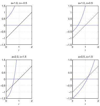
Figure 1. The polynomial $p(r)$ and its relation to the line $L$ for different values of $a$ and $c$.

1. $c<0$. In this case $p(r)>r-1$ and $p(r)>0$ for all $r\geq 0$, so there are no extremal surfaces and no singularities. The surfaces exist for all $r$ and they are space-like.

2. $0<c<1$. Again, $p(r)>r-1$ but $p(r)$ becomes negative for small values of $r$. There is a zero at a value $r_{0}\leq c<1$. So the surfaces in this case have a minimal surface but no singularity. The hypersurfaces are space-like. They come in from null-infinity reach a minimal hypersurface at $r_{0}$ and then extend out again to null-infinity.

3. $c>1$. This is a more complicated case. For all values of $a$ the polynomial $p$ has a zero at a value $r=r_{0}$ and intersects the line $L$ at a value $r=r_{1}$. We have to distinguish two subcases:

   1. $1<c<1+a^{2}$. In this case $r_{1}<r_{0}<1$. The hypersurfaces exist in the region $0\leq r\leq r_{1}$ where they are time-like and $r_{0}\leq r$ where they are space-like. The time-like hypersurfaces reach the Schwarzschild singularity at $r=0$ and grow towards larger radii but stop at $r_{1}<1$ where their extrinsic curvature diverges. The space-like hypersurfaces come in from null-infinity and, crossing the horizon, reach a minimal surface with radius $r_{0}$. Then they go out again to null-infinity.

   2. $1+a^{2}<c$. Here $1<r_{0}<r_{1}$ and the two regions for existence of the hypersurfaces are reversed. The hypersurfaces on $0\leq r\leq r_{0}$ extending from the singularity are time-like, grow towards a surface of maximal radius and then shrink back to $r=0$. The outer hypersurfaces on $r_{1}\leq r$ are space-like, come in from null-infinity and end at $r_{1}$ with a diverging extrinsic curvature.

4. Embedding CSC slices in Kruskal space-time

The Kruskal extension of the Schwarzschild space-time is covered by coordinates $X$ and $T$ which are related to the Schwarzschild coordinates by the relations

(17) $$e^{r}(r-1)=X^{2}-T^{2},\qquad t=\log\left(\frac{X+T}{X-T}\right).$$

In these coordinates the metric takes the form

$$\frac{4e^{-r}}{r}\left(-\mathrm{d}T^{2}+\mathrm{d}X^{2}\right)+r^{2}\mathrm{d}\sigma^{2},$$

where $r$ has to be regarded as a function of $X^{2}-T^{2}$ via (17).

4.1. The embedding equation

To obtain the embedding equation in terms of the Kruskal coordinates we write $r$ and $t$ as functions of some parameter $s$, so that $t(s)=h(r(s))$, and then regard also $T$ and $X$ as functions of $s$. Using the relationship between the coordinates and the embedding equation one derives the equations

$$\dot{T} =\frac{1}{2}\left(Xh^{\prime}(r)+Tr/(r-1)\right)\dot{r},$$

$$\dot{X} =\frac{1}{2}\left(Th^{\prime}(r)+Xr/(r-1)\right)\dot{r}.$$

With $h^{\prime}(r)=Q(r)r/(r-1)$ one derives easily the equation for the height function $T=T(X)$ as

(18) $$\frac{dT}{dX}=\frac{QX+T}{X+QT},$$

from which it is obvious, that the horizon at $r=1$ is not a concern. From this form of the embedding equation one quickly derives the following symmetry properties of the solutions. If $T(X)$ is a solution of the equation with $Q=\sqrt{q/p}$ taken from the positive branch of the square root, then $-T(X)$ is a solution for $-Q$. Similarly, if $T(X)$ is a solution for positive $Q$, then $\bar{T}(X)=T(-X)$ is a solution for $-Q$.

In order to derive further properties we write down the embedding equation in parametric form by choosing $s/2$ as the geodesic distance along the radial directions and we arrive at the system

$$(r-1)\,\dot{T} =\left(\sqrt{r|q(r)|}X+\sqrt{r|p(r)|}T\right),$$

$$(r-1)\,\dot{X} =\left(\sqrt{r|q(r)|}T+\sqrt{r|p(r)|}X\right).$$

In terms of the null coordinates $U=T-X$ and $V=T+X$ this system can be written as

(19) $$(r-1)\,\dot{U} =\left(\sqrt{r|p(r)|}-\sqrt{r|q(r)|}\right)U,$$

$$(r-1)\,\dot{V} =\left(\sqrt{r|p(r)|}+\sqrt{r|q(r)|}\right)V.$$

We list some of the obvious properties of the system:

1. In the asymptotic region $r\to\infty$ we have

   $$\dot{U}\approx 0,\qquad\dot{V}\approx 2ar^{2}\,V,$$

   which implies that the hypersurfaces approach the light cones $U=const$ for large $r$.

2. Similarly, for large values of the parameter $a$ the hypersurfaces approach null hypersurfaces. This can easily be seen already from the form of the metric (1). With $g_{rr}=\frac{r}{p(r)}$ it is clear that the metric degenerates for $a\to\infty$.

3. Note that the case $h^{\prime}(r)\to 1$ for $r\to\infty$ referred to in sect 3.1 corresponds to a hypersurface which approaches future null-infinity for large values of $X$, while the case $h^{\prime}(r)\to-1$ gives a hypersurface approaching future null-infinity in the other asymptotic region of the Kruskal extension where $X<0$. This implies that for hypersurfaces connecting both null-infinities we have to consider $Q$ and $-Q$.

4. Changing the branch of $\sqrt{r|q(r)|}$ corresponds to the interchange of $U$ and $V$, i.e. to $X\mapsto-X$. Similarly, the system is invariant under the transformation $(U,V)\mapsto(-U,-V)$. These transformations together correspond to the $T\mapsto-T$. So we can restrict ourselves to consider only hypersurfaces which lie in the region $U<0$, corresponding to the regions I and III in the standard Kruskal extension.

5. At the extremal surfaces given by $p(r)=0$ we have

   $$\frac{\dot{U}}{U}=-\frac{\dot{V}}{V}\,,\qquad\frac{\dot{T}}{\dot{X}}=\frac{X}{T}\,.$$

   This means that at these points $\frac{d(UV)}{ds}=0$, so that the hypersurfaces touch the hypersurface $r=const\,$ at these points.

6. At the locations with $q(r)=0$, where the extrinsic curvature of the hypersurfaces diverges, we have

   $$\frac{\dot{U}}{U}=\frac{\dot{V}}{V}\,,\qquad\frac{\dot{T}}{\dot{X}}=\frac{T}{X}\,.$$

   In this case, the condition implies that $\frac{d(T/X)}{ds}=0$, i.e. the hypersurfaces touch the hypersurface $t=const\,$ through that point.

4.2. Behaviour at the horizon

The horizon at $r=1$ corresponds to the two null lines in the Kruskal extension defined by either $U=0$ or $V=0$. In order to see the behaviour of the system close to these lines we need to expand the function $r(U,V)$ for small $U$, respectively $V$. We make the discussion for the case where $p$ and $q$ are positive, an analogous argument applies to the case where they are negative. We have

$$y=-UV=e^{r}(r-1)=e\left((r-1)+(r-1)^{2}+\frac{1}{2}(r-1)^{3}+\mathcal{O}(r-1)^{4}\right)\,,$$

which can be inverted to

$$(r-1)=(y/e)-(y/e)^{2}+\frac{3}{2}(y/e)^{3}+\mathcal{O}(y^{4})\,.$$

Furthermore, near $r=1$ we have (in the generic case $\sqrt{1+a^{2}-c}\neq 0$)

$$\begin{gathered}\sqrt{rq(r)}-\sqrt{rp(r)}=\frac{r-1}{2\,{\sqrt{1+a^{2}-c}}}+\frac{1-4\,a^{2}-2\,c}{8\,{\left(1+a^{2}-c\right)}^{\frac{3}{2}}}\;(r-1)^{2}+{\mathcal{O}(r-1)^{3}},\\ \sqrt{rq(r)}+\sqrt{rp(r)}=2\,{\sqrt{1+a^{2}-c}}+\frac{3+8\,a^{2}-2\,c}{2\,{\sqrt{1+a^{2}-c}}}\;(r-1)+{\mathcal{O}(r-1)}^{2}.\end{gathered}$$

Thus, near $r=1$ the system can be written as

$$\dot{U} =\frac{U}{2\,{\sqrt{1+a^{2}-c}}}-\frac{1-4\,a^{2}-2\,c}{8e\,{\left(1+a^{2}-c\right)}^{\frac{3}{2}}}\;U^{2}V+\mathcal{O}(U^{2}V^{2})\,,$$

$$\dot{V} =-\frac{2e\,{\sqrt{1+a^{2}-c}}}{U}+\frac{7+12\,a^{2}-6\,c}{2\,{\sqrt{1+a^{2}-c}}}\;V+{\mathcal{O}(UV)}\,.$$

Clearly, in the neighbourhood of $V=0$ the system is regular and has regular solutions. The hypersurfaces determined by the system cross the horizon $V=0$ in a regular way. However, the horizon at $U=0$ is different. In this case there is no way to approach the horizon because the equation becomes singular at $U=0$.

The behaviour at the two horizons $U=0$, i.e. $T=X$, and $V=0$, i.e. $T=-X$, can be obtained directly from equation (18). Since $Q$ is positive, we find that $T=X$ is a solution, while $T=-X$ is not a solution. This implies, by uniqueness of solution, that $T=X$ cannot be crossed by other solutions, while $T=-X$ can be crossed.

4.3. Discussion of the different cases

Let us now discuss the different cases found in the previous section and determine the generic behaviour of the hypersurfaces.

4.3.1. The case $c<0$

In this case $p$ and $q$ have no zeros and $\sqrt{rp(r)}>\sqrt{rq(r)}$ for $r>1$, while $\sqrt{rp(r)}<\sqrt{rq(r)}$ for $r<1$. Thus, it is easy to see that $\dot{U}>0$ for $U<0$ and $\dot{V}>0$ for $V>0$. This implies that a hypersurface which happens to get into region I where $U<0$ and $V>0$ will approach $U=0$ for large positive values of $s$, while in the other direction it will approach $V=0$ and, because the equation is regular there, it will cross into region III, the white hole region, where $V<0$ and hence $\dot{V}>0$. So, in this case, the hypersurfaces emerge from the white hole and extend all the way out towards null-infinity.

In Fig. 2 we show hypersurfaces for $c=-0.5$. We exhibit three different classes of hypersurfaces. Within each class there are three hypersurfaces with different values of $a$ which go through the same space-time event. The values of $a$ are $a=10$, $a=1$, and $a=0.01$. It can be clearly seen that the large values of $a$ result in an almost null hypersurface.

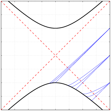
Figure 2. Three classes of hypersurface in different regions of space-time for the case $c=-0.5$. Within each class the parameter $a$ takes the values $a=10$, $a=1$, and $a=0.01$.

4.3.2. The case $c=0$

This case is almost the same as the case $c<0$. Also in this case the hypersurfaces from any space-time event emerge from the singularity at $r=0$ except that now the location $r=0$ is also a point where $\dot{r}=0$, so it is a minimal surface. The hypersurfaces run into the singularity tangentially.

4.3.3. The case $0<c<1$

In this case the polynomial $p(r)$ vanishes at $r=r_{0}$ between $r=0$ and $r=1$. So a corresponding hypersurface has a minimal surface. At that minimal surface the geometry of the hypersurface is completely regular. The hypersurface which is space-like comes in from null-infinity at large positive values of $X$, and touches the hypersurface of constant radius $r=r_{0}$ in a minimal surface. TYhere the solution switches the branch and continues on into region IV where it ultimately reaches the other future null-infinity. Along the way it smoothly crosses both horizons. Since one branch of the solution only covers the part of the hypersurface up to the minimal surface, the complete hypersurface is obtained by switching the branch of $\sqrt{p(r)}$ at the minimal surface. All the hypersurfaces in this case connect one null-infinity with the other. They all lie below the throat at $\,T=0=X$.

Again, for large values of $a$ the hypersurfaces approach null-hypersurfaces. In this case these are two null-hypersurfaces intersecting in the minimal sphere at $r=r_{0}$ outside the singularity. In Fig. 3 we show again a sample of hypersurfaces with $c=0.5$ and the same values for $a$ and initial conditions as in Fig. 2.

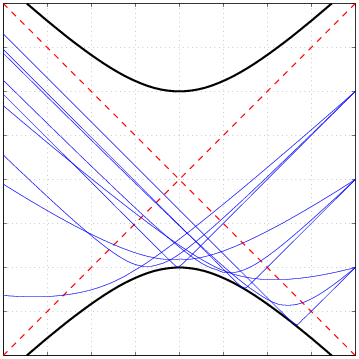
Figure 3. The case $0<c<1$

4.3.4. The case $c=1$

In this case, as in the previous case, the polynomial $p(r)$ vanishes between $r=0$ and $r=1$. The additional feature is the emergence of a point where $q(r)$ vanishes. For the special case $c=1$ treated here this location is at the singularity. The hypersurfaces with $a\neq 0$ have the same qualitative behaviour is the ones treated in the previous case. This case yields hypersurfaces with constant mean curvature and constant scalar curvature (considered by Schmidt [9], see also Brill et al. [5]) for which the extrinsic curvature is pure trace $K_{ab}=Kg_{ab}$.

The case $a=0$ is interesting because then $q$ vanishes identically so that the solutions of the system are

$$T/X=const\,,$$

which are the asymptotically euclidean hypersurfaces $t=const\,$ of the Schwarzschild space-time.

4.3.5. The case $c>1$

Now the polynomial $p(r)$ starts out below the line $L$ and (for all non-zero values of $a$) there is an intersection with this line at $r=r_{1}$. This intersection may lie below $r=1$ or above $r=1$ depending on the parameters $a$ and $c$. The critical case is given by $a^{2}=c-1$. We first discuss the case $1<c<1+a^{2}$. Then the intersection is inside $r=1$ and the polynomial hits the $r$-axis at a value $r=r_{0}>r_{1}$ after intersecting the line. Hypersurfaces exist for all values of $r\geq r_{0}$. Again, the geometry at the minimal surface $r=r_{0}$ is regular so we can continue the hypersurface by switching to the other branch of $\sqrt{p(r)}$. We get again the same qualitative behaviour of the hypersurfaces. They connect one null-infinity with the other. Some of the hypersurfaces are shown in Fig. 4.

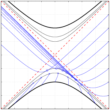
Figure 4. The case $1<c<1+a^{2}$. We show the hypersurfaces for fixed values of $a$ and $c$, varying their location in space-time.

The other region of existence for hypersurfaces is inside the horizon. These hypersurfaces are time-like. They emerge from the singularity and grow towards the future until they come to an end when $q$ vanishes, i.e. when the extrinsic curvature diverges.

The other case is when $1+a^{2}<c$. In this case we have space-like hypersurfaces in region I which end with a diverging extrinsic curvature, see Fig. 5, and there are time-like hypersurfaces which come out of the white hole singularity, grow up to a maximal surface and then, after switching to the other branch of $\sqrt{p(r)}$, they fall into the black hole singularity, see Fig. 5.

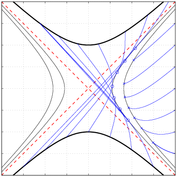
Figure 5. The case $1+a^{2}<c$. Hypersurfaces for fixed values of $a$ and $c$, and varying location in space-time.

Finally, in the critical case when $1+a^{2}=c\,$ the zeros of $p(r)$ and $q(r)$ coincide at $r=1$, the origin $T=0=X$ is a point where the system (19) is singular. This follows from the fact that

$$\sqrt{rp(r)}\pm\sqrt{rq(r)}=\sqrt{r-1}\left(\sqrt{r+a^{2}(1+r+r^{2})}\pm\sqrt{a^{2}(1+r+r^{2})}\right)\,,$$

where the expression in parentheses is differentiable in $r$ near $r=1$. Using the coordinate transformation between Schwarzschild and Kruskal coordinates we see that in the region I the system can be written in the form

(20) $$\dot{U} =\left\{\sqrt{e}\left(\sqrt{3a^{2}}-\sqrt{1+3a^{2}}\right)+\text{reg}(U,V)\right\}\frac{\sqrt{-U}}{\sqrt{V}}\,,$$

$$\dot{V} =\left\{\sqrt{e}\left(\sqrt{3a^{2}}+\sqrt{1+3a^{2}}\right)+\text{reg}(U,V)\right\}\frac{\sqrt{V}}{\sqrt{-U}}\,,$$

where $\text{reg}(U,V)$ stands for a function which is regular near $U=V=0$ and vanishes there. Near the origin the behaviour of the solutions is given by this first exhibited term. Dropping the regular term we arrive at the system

(21) $$\dot{U} =\left\{\sqrt{e}\left(\sqrt{3a^{2}}-\sqrt{1+3a^{2}}\right)\right\}\frac{\sqrt{-U}}{\sqrt{V}}\,,$$

$$\dot{V} =\left\{\sqrt{e}\left(\sqrt{3a^{2}}+\sqrt{1+3a^{2}}\right)\right\}\frac{\sqrt{V}}{\sqrt{-U}}\,,$$

which has the solution

(22) $$\begin{aligned} U(s)=U_{0}\left(1+\frac{\sqrt{1+3a^{2}}}{\sqrt{-U_{0}V_{0}}}s\right)^{1-\gamma}\,,\\ V(s)=V_{0}\left(1+\frac{\sqrt{1+3a^{2}}}{\sqrt{-U_{0}V_{0}}}s\right)^{1+\gamma}\,,\end{aligned}\qquad\gamma=\frac{\sqrt{3a^{2}}}{\sqrt{1+3a^{2}}}<1\,.$$

Following the hypersurface backward for $s<0$ from any initial point $(U_{0},V_{0})$ we find that at $s=-\sqrt{-U_{0}V_{0}}/\sqrt{1+3a^{2}}$ both $U$ and $V$ become zero, the hypersurface runs into the origin and stops there. The singularity at the origin therefore has the consequence that uniqueness of the solution is lost, see Fig. 6

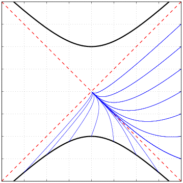
Figure 6. The case $c=1+a^{2}$ for $a^{2}=0.1$

5. Discussion

In this paper we have discussed the class of spherically symmetric hypersurfaces with constant scalar curvature embedded in the Schwarzschild space-time. We found several types of hypersurfaces with qualitatively different behaviour. We have looked at this class of hypersurfaces because we were interested in finding ways of slicing the Schwarzschild space-time with hypersurfaces which become asymptotically hyperboloidal, i.e. for which the scalar curvature approaches a negative constant for large radii.

We can now see that for the subclass of space-like hypersurfaces with $0<c<1+a^{2}$ one might be able to achieve this. All of these hypersurfaces connect the two future null-infinities of the Kruskal extension. Hypersurfaces with $c<0$ could foliate the regions I and III, i.e. the white hole and the asymptotic region. However, note that the hypersurfaces shown in Fig. 3 and Fig. 4 do not form a foliation because they intersect. So one needs to vary the available parameters $a$ and $c$, as well as the location of the hypersurface in the space-time, in order to avoid intersections. To illustrate this we display in Fig. 7

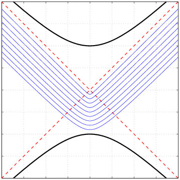
Figure 7. A set of symmetric hypersurfaces for fixed $a=1$ and equidistant intersection with the $T$-axis.

several hypersurfaces with the fixed value of $a=1$ that are symmetric under $X\mapsto-X$. So they have their minimal surface on the $T$-axis. From the intersection of the hypersurfaces with this axis we can determine the corresponding value of $c$. In this part of the space-time the family of hypersurfaces seems to give a foliation, although we have not proved this. Discussions of these issues will be left to another paper.

6. Acknowledgments

We are grateful to E. Malec and N. O’Murchadha for discussions and hints. This work was supported in part by the Deutsche Forschungsgemeinschaft (DFG).

References

- [1] R. Penrose. Asymptotic properties of fields and space-times. Phys. Rev. Lett., 10(5), p. 66–68, 1963.
- [2] H. Friedrich. Cauchy problems for the conformal vacuum field equations in general relativity. Comm. Math. Phys., 91, p. 445–472, 1983.
- [3] H. Friedrich. On the existence of n-geodesically complete or future complete solutions of Einstein’s field equations with smooth asymptotic structure. Comm. Math. Phys., 107, p. 587–609, 1986.
- [4] J. Frauendiener. Conformal infinity. Living Rev. Relativity, 7, 2004. http://www.livingreviews.org/lrr-2004-1.
- [5] D. R. Brill, J. M. Cavallo, and J. A. Isenberg. -surfaces in the Schwarzschild space-time and the construction of lattice cosmologies. J. Math. Phys., 21, p. 2789–2796, 1980.
- [6] N. O’Murchadha and E. Malec. Constant mean curvature slices in the extended Schwarzschild solution and the collapse of the lapse. Phys. Rev. D, 68, p. 124019, 2003.
- [7] C. W. Misner and D. H. Sharp. Relativistic equations for adiabatic, symmetric gravitational collapse. Phys. Rev. B, 136, p. 571–576, 1964.
- [8] R. M. Wald. General Relativity. Chicago University Press, Chicago, 1984.
- [9] B. Schmidt. Data for the numerical calculation of the Kruskal space-time. In J. Frauendiener and H. Friedrich, editors, The conformal structure of space-times: geometry, analysis, numerics, volume 604 of Lecture Notes in Physics, pages 283–295. Springer-Verlag, Heidelberg, 2002.