Simulation of Acoustic Black Hole in a Laval Nozzle

Abstract

A numerical simulation of fluid flows in a Laval nozzle is performed to observe the formation of an acoustic black hole and the classical counterpart to Hawking radiation under a realistic setting of the laboratory experiment. We aim to construct a practical procedure of the data analysis to extract the classical counterpart to Hawking radiation from experimental data. Following our procedure, we determine the surface gravity of the acoustic black hole from obtained numerical data. Some noteworthy points in analyzing the experimental data are clarified through our numerical simulation.

I Introduction

The existence of the black hole horizon is essential to the Hawking radiation Hawking (1975); Birrell and Davis (1982); Visser (2003); Unruh and Schtzhold (2005). The horizon causes an extremely large redshift on an outgoing wave of a matter field during propagating from a vicinity of the horizon to the asymptotically flat region. This redshift results in the Planckian distribution of quantum mechanically created particles at the future null infinity. Although the Hawking radiation has not yet been confirmed observationally, it has been pointed out that the similar phenomenon appears on phonons in a transonic flow of a fluid. This theoretical phenomenon in the fluid is called the sonic analogue of Hawking radiation, and the transonic fluid flow on which the sonic analogue of Hawking radiation occurs is called the acoustic black hole Unruh (1981, 1995); Visser (1998); Volovik (1999); Novello et al. (2002); Barceló et al. (2003, 2004, 2005). In the transonic flow, the boundary between a subsonic and a supersonic region is the sonic point. The sonic point corresponds to the black hole horizon and called the sonic horizon. The region apart form the sonic point in the subsonic region corresponds to the asymptotically flat region in a black hole spacetime. The sound wave which propagates from a vicinity of the sonic point to the subsonic region receives the extremely large redshift and the sonic analogue of Hawking radiation appears on phonons. The Hawking temperature $T_{H}$ of the acoustic black hole is given by the gradient of the fluid velocity at the sonic point $x=x_{s}$ Unruh (1981):

$$T_{H}=\frac{\hbar\,c_{s}}{2\pi k_{B}}\left.\frac{d}{dx}\left(\frac{v}{c_{s}}\right)\right|_{x=x_{s}}\,,$$ (1)

where $c_{s}$ and $v$ are the sound velocity and the fluid velocity, respectively. For an ordinary system with typical size $\sim 1$ m and $c_{s}\sim 340$ m/s, we obtain $T_{H}\sim 4\times 10^{-10}$ K. Thus, in a practical experiment in a laboratory, it is very difficult to detect the sonic analogue of Hawking radiation with such an extremely low temperature.

While it is very hard to detect the sonic analogue of Hawking radiation on phonons, which is a quantum origin, a classical sound wave with a sufficiently large amplitude can be available for detecting the effect of the acoustic black hole on a propagation of sound waves in practical experiments. Indeed, the thermal nature of Hawking radiation is not a quantum origin; it comes from a large redshift on the wave propagating from a vicinity of the horizon to the asymptotically flat region, and has nothing to do with the quantum effect (see Appendix). Therefore, if we can construct a classical quantity from sound waves which shows the thermal distribution, then such a quantity can be interpreted as a classical counterpart to Hawking radiation. A candidate for the classical counterpart has already been introduced in the references Nouri-Zonoz and Padmanabhan (1998); Sakagami and Ohashi (2002) by using a Fourier component of an outgoing wave from a vicinity of the horizon.

By the way, since a realistic fluid is composed of molecules, the effect of the molecule size discrepancy of the fluid becomes one of the important issues of the acoustic black hole. This effect appears in the modified dispersion relation at high energies of phonons. However, in the expansion by the molecule size discrepancy, the zeroth order form of the quantum expectation value of the number operator $\left<0\right|N\left|0\right>$ of phonons results in the thermal spectrum at least not so high energy region. That is, the effect of the molecule size discrepancy is not dominant in the sonic analogue of Hawking radiation. Therefore, before proceeding to the issue of the molecule size discrepancy, it is necessary to detect the ordinary Hawking radiation (thermal spectrum) by a real experiment in laboratory, and the molecule size discrepancy is not in the scope of this paper. Hence we concentrate on the construction of the practical procedure to extract the evidence of the Hawking radiation (thermal spectrum) from the experimental data. To do so, we make use of the classical counterpart to Hawking radiation.

We should emphasize here that the Hawking temperature (1) includes the Planck constant $\hbar$ and we can not consider the temperature $T_{H}$ in discussing the “classical” counterpart to Hawking radiation. However we can consider the surface gravity $\kappa$ of the black hole horizon which is a purely classical quantity and relates to the Hawking temperature as $k_{B}\,T_{H}=\hbar\,\kappa/2\pi$. Hence, for the acoustic black hole, we consider the surface gravity $\kappa_{H}$ of the sonic horizon instead of the Hawking temperature,

$$\kappa_{H}=c_{s}\left.\frac{d}{dx}\left(\frac{v}{c_{s}}\right)\right|_{x=x_{s}}\,.$$ (2)

In this paper, we aim to construct a practical procedure of the data analysis to obtain the classical counterpart to Hawking radiation in a realistic setting of the acoustic black hole. To do so, we perform a numerical simulation of a fluid flow in a practical experimental setting, and demonstrate that our procedure works well to detect the classical counterpart to Hawking radiation.

We organize the paper as follows. In the section II, we review the acoustic black hole in a Laval nozzle and define the classical counterpart to Hawking radiation. The section III is devoted to the introduction of our numerical method to simulate a transonic flow, and to the construction of the practical procedure of the data analysis. In the section IV, our numerical results are presented and we determine the surface gravity of the sonic horizon. Finally the summary and conclusion are in the section V.

II Acoustic black hole with a Laval nozzle

We consider an acoustic black hole with a fluid in a Laval nozzle as proposed in Sakagami and Ohashi (2002). The Laval nozzle, as shown in the right panel in FIG. 1, has a throat where the cross section of the nozzle becomes minimum. The fluid is accelerated from the up stream to the down stream and the flow has the sonic point at the throat when a sufficiently large velocity is given at the inlet of the nozzle. Even if we prepare an initial flow which has no sonic point (e.g. the lower part of the right panel in FIG. 1), the flow can settle down to a stationary transonic flow (e.g. the upper part of the right panel in FIG.  1) with appropriate boundary conditions at the inlet and the outlet of the nozzle. This is the sonic analogue model which corresponds to the gravitational collapse.

Here we note that, if a stationary transonic flow is prepared from the beginning (which corresponds to the eternal black hole), we can not expect to obtain the classical counterpart to the Hawking radiation; for the eternal case, the tunneling of phonons across the sonic point can result in the Hawking radiation and this is the purely quantum effect. Hence, when we are interested in the “classical” counterpart to Hawking radiation, it is necessary to consider the situation of the sonic point formation in course of the dynamical evolution of the fluid flow . As seen below, the sound wave which is prepared on the fluid flow before the formation of the sonic point becomes the classical counterpart to the quantum fluctuation which causes the classical counterpart to Hawking radiation.

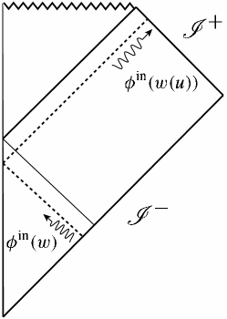
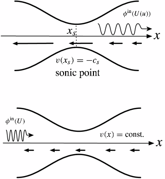
Figure 1: Propagation of waves in a spacetime of gravitational collapse and in a Laval nozzle.

II.1 Basic equations

We consider a perfect fluid and treat the flow in a Laval nozzle as one dimensional for simplicity. The basic equations are the mass conservation equation and the Euler equation:

$$\partial_{t}\rho+\frac{1}{S}\partial_{x}\left(\rho vS\right)=0,$$ (3a)

$$\rho\left(\partial_{t}v+v\partial_{x}v\right)=-\partial_{x}p,$$ (3b)

where $\rho(t,x)$ is the mass density, $v(t,x)$ is the fluid velocity, $p(t,x)$ is the pressure of the fluid and $S(x)$ is the cross section of the Laval nozzle. We assume the adiabatic ideal gas type equation of state $p\propto\rho^{\gamma}$ where $\gamma$ is the adiabatic index. The sound velocity $c_{s}$ is given by

$$c_{s}^{2}\equiv\dfrac{dp}{d\rho}\propto\rho^{\gamma-1}.$$ (4)

For a stationary background flow, we can obtain the sound velocity $c_{s}$ and the cross section $S$ of the nozzle as a function of the Mach number $M=v/c_{s}$ of the flow:

$$c_{s}=c_{{\text{in}}}\left(\frac{M^{2}+\frac{2}{\gamma-1}}{M_{\text{in}}^{2}+\frac{2}{\gamma-1}}\right)^{-1/2},\quad S=S_{\text{in}}\frac{M_{\text{in}}}{M}\left(\frac{M^{2}+\frac{2}{\gamma-1}}{M_{\text{in}}^{2}+\frac{2}{\gamma-1}}\right)^{\frac{\gamma+1}{2(\gamma-1)}},$$ (5)

where quantities with subscript “in” represent the values at the inlet of the nozzle. The spatial derivative of the Mach number at the sonic point $x=x_{s}$ is

$$\left.\frac{dM}{dx}\right|_{x_{s}}=\pm\left.\sqrt{\frac{(\gamma+1)}{4}\frac{1}{S}\left(\frac{d^{2}S}{dx^{2}}\right)}\right|_{x_{s}},$$ (6)

and this value relates to the surface gravity of the sonic horizon by Eq. (2). Figure 2 shows the structure of the stationary flow for $\gamma=7/5$ and $S(x)=2-\cos(\pi x)$. Here we set that the inlet is at $x=1$, the throat at $x=0$ and the outlet at $x=-1$. That is, the fluid flows downward from $x=1$ to $x=-1$, then $M<0$ and FIG. 2 shows the absolute value of $M$. The boundary condition is given by the Mach number $M_{\text{in}}$ at the inlet of the nozzle, and each line in FIG. 2 corresponds to a different value of $M_{\text{in}}$. The blue line which passes the sonic point $(x,M)=(0,1)$ is given by $M_{\text{in}}=M_{*}\approx-0.197$ and represents the stationary transonic flow. For the case $c_{\text{in}}=1$, we find

$$\left.\frac{dM}{dx}\right|_{x=0}=\pm\sqrt{\frac{3}{5}}\,\pi,\quad c_{s}|_{x=0}=(3|M_{*}|)^{1/6},$$ (7)

and the surface gravity given by Eq. (2) is

$$\frac{\kappa_{H}}{2\pi}=\frac{(3|M_{*}|)^{1/6}}{2\pi}\sqrt{\frac{3}{5}}\,\pi\approx 0.355.$$ (8)

Here it should be emphasized that, because the cross section of the nozzle is set $S(x)=2-\cos(\pi x)$ with $-1<x<1$, the spatial scale is normalized by $L/2$, where $L$ is the length of the nozzle, and that the temporal scale is normalized by $L/(2c_{\text{in}})$, where we set $c_{\text{in}}=1$.

We have not considered the perturbation of the fluid flow so far. In the following sections, the perturbation (sound wave) is introduced on the fluid flow, and the classical counterpart to Hawking radiation is defined. Then in the section IV, we compare this surface gravity (8) with the surface gravity of the sonic horizon which is obtained through the observation of the classical counterpart to Hawking radiation in our numerical simulation.

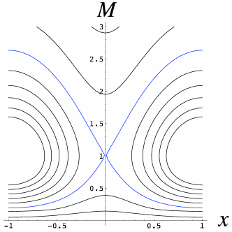
Figure 2: Absolute value of the Mach number as a function of a spatial coordinate $x$. Each line represents the stationary solution of the flow with different boundary value $M_{in}$. The blue lines represent transonic flows.

II.2 Classical counterpart to Hawking radiation

As originally shown in the reference Unruh (1981), the perturbation of the velocity potential for the transonic fluid flow obeys the same equation as a massless free scalar field in a black hole spacetime. Therefore the classical counterpart to Hawking radiation of the acoustic black hole in the Laval nozzle should be observed by the sound wave on the transonic fluid flow. The most important sound wave is the one which starts to propagate against the stream from the outlet of the nozzle before the formation of the sonic point (the lower part of the right panel in FIG.  1) and passes through the throat just before the moment of the sonic point formation to reach the inlet of the nozzle (the upper part of the right panel in FIG. 1). This sound wave receives the extremely large redshift which will cause the classical counterpart to Hawking radiation.

When the fluid flow is irrotational and we introduce the velocity potential $\Phi$ which relates with the fluid velocity as $v=\partial_{x}\Phi$, the evolution equation of the perturbation $\phi$ of $\Phi$ is obtained from Eqs. (3),

$$\frac{1}{S\,\rho}\left[\partial_{t}+\partial_{x}v\right]\left(\frac{S\,\rho}{c_{s}^{2}}\right)\left[\partial_{t}+v\partial_{x}\right]\phi-\frac{1}{S\,\rho}\partial_{x}\!\left(S\,\rho\partial_{x}\phi\right)=0.$$ (9)

This corresponds to the Klein-Gordon equation $\square\phi=0$ with the acoustic metric

$$ds^{2}=\left(\frac{S\,\rho}{c_{s}}\right)\left[-(c_{s}^{2}-v^{2})dt^{2}-2v\,dt\,dx+dx^{2}+dy^{2}+dz^{2}\right],$$ (10)

where the location of the sonic horizon (sonic point) $x=x_{s}$ is given by $c_{s}(x_{s})^{2}=v(x_{s})^{2}$. Here we should note that, because we consider the one dimensional flow along $x$-axis as mentioned at the beginning of the previous section II.1, the two dimensional section of $(y,z)$ coordinate is omitted in obtaining Eq. (9) from $\square\phi=0$. In the following analysis, we omit the two dimensional section of $(y,z)$ coordinate.

In order to describe the extremely large redshift which causes the classical counterpart to Hawking radiation, we introduce the following null coordinates for the first,

$$u=t-\int\frac{dx}{c_{s}+v},\quad w=t+\int\frac{dx}{c_{s}-v},$$ (11)

and the acoustic metric becomes $ds^{2}=\left(S\,\rho/c_{s}\right)\left(c_{s}^{2}-v^{2}\right)du\,dw$, which has a coordinate singularity at $x=x_{s}$. In order to eliminate the coordinate singularity, we introduce the new null coordinates

$$U=-\frac{1}{c_{s0}^{\prime}+v_{0}^{\prime}}\exp\left[-(c_{s0}^{\prime}+v_{0}^{\prime})u\right],\quad W=\frac{1}{c_{s0}^{\prime}+v_{0}^{\prime}}\exp\left[(c_{s0}^{\prime}+v_{0}^{\prime})w\right],$$ (12)

where ${}^{\prime}=\partial_{x}$ and quantities with subscript $0$ denotes values at the sonic point $x=x_{s}$. Then the acoustic metric and the evolution equation (9) of the perturbation $\phi$ become

$$ds^{2} =-\left(\frac{S\,\rho}{c_{s}}\right)\,(c_{s}^{2}-v^{2})\,\exp\left[-2(c_{s0}^{\prime}+v_{0}^{\prime})\int\frac{c_{s}\,dx}{c_{s}^{2}-v^{2}}\right]\,dU\,dW\equiv-F\,dU\,dW,$$ (13)

$$\square\phi =\frac{1}{F}\partial_{UW}\,\phi=0.$$ (14)

The form of this metric near the sonic horizon is $ds^{2}\approx-2S_{0}\rho_{0}(c_{s0}^{\prime}+v_{0}^{\prime})\,dU\,dW$, where $c_{s}^{2}-v^{2}\approx 2c_{s0}(c_{s0}^{\prime}+v_{0}^{\prime})x$ is used. This denotes explicitly that the coordinate $(U,W)$ does not have coordinate singularities and corresponds to the Kruskal-Szekeres coordinate of the Schwarzschild spacetime. Here it should be recalled that, in the spacetime of the gravitational collapse (the left panel in FIG. 1), the Kruskal-Szekeres coordinate is appropriate to describe the rest observer at the spacetime region before the formation of the black hole Birrell and Davis (1982). Hence the outgoing normal mode of the sound wave which corresponds to the zero point fluctuation of the quantized matter field before the formation of the black hole (i.e. the mode function on the flat spacetime) is given by

$$\phi^{\text{in}}(U)=A_{\phi}\,e^{-i\omega_{0}U},$$ (15)

where $\omega_{0}$ is the initial frequency and $A_{\phi}$ is the amplitude of this mode. In the original coordinate $(t,x)$, this mode behaves as

$$\phi^{\text{in}}(U(u))=\phi^{\text{in}}(t,x)=A_{\phi}\exp\left[\frac{i\omega_{0}}{c_{s0}^{\prime}+v_{0}^{\prime}}\exp\left(-(c_{s0}^{\prime}+v_{0}^{\prime})\left(t-\int^{x}\frac{dx}{c_{s}+v}\right)\right)\right].$$ (16)

This yields the temporal wave form at the observation point $x=x_{\text{obs}}$ in the asymptotic region:

$$\phi^{\text{out}}(t)\equiv\phi^{\text{in}}(t,x_{\text{obs}})=A_{\phi}\exp\left[\frac{i\omega_{0}}{c_{s0}^{\prime}+v_{0}^{\prime}}\exp\left(-(c_{s0}^{\prime}+v_{0}^{\prime})\left(t-\int^{x_{\text{obs}}}\frac{dx}{c_{s}+v}\right)\right)\right].$$ (17)

Fourier component of this mode is defined by

$$\phi_{\omega}^{\text{out}}=\int_{-\infty}^{\infty}dt\,\phi^{\text{out}}(t)e^{i\omega t},$$ (18)

and the power spectrum is

$$P(\omega)=\left|\phi_{\omega}^{\text{out}}\right|^{2}=\left(\frac{A_{\phi}^{2}}{\omega_{H}\,\omega}\right)\frac{e^{\omega/\omega_{H}}}{e^{\omega/\omega_{H}}-1}\qquad(-\infty<\omega<+\infty),$$ (19)

where the quantity $\omega_{H}$ is defined by

$$\omega_{H}\equiv\frac{\kappa_{H}}{2\pi}=\frac{c_{s0}}{2\pi}\frac{d}{dx}\!\left(\frac{v}{c_{s}}\right)_{0}.$$ (20)

Here it should be noted that, because the existence of the sonic point is assumed in the above discussion, the form of $P(\omega)$ of Eq. (19) must be obtained after the formation of the sonic horizon in the fluid flow.

One may think it is strange that the initial frequency $\omega_{0}$ does not appear in the power spectrum (19). It is the fact that the initial frequency $\omega_{0}$ does appear in the power spectrum in the context of the quantum field theory, because the amplitude $A_{\phi}$ is determined by the normalization condition for the mode functions to be $A_{\phi}\propto 1/\sqrt{\omega_{0}}$. However, in the calculation for the classical counterpart to Hawking radiation, the initial frequency $\omega_{0}$ appears only in the phase of the Fourier component $\phi_{\omega}^{\text{out}}$ and the power $P(\omega)$ does not explicitly depend on $\omega_{0}$.

The power spectrum (19) has the Planckian distribution for $\omega<0$ and this is the classical counterpart to the quantum Hawking radiation Nouri-Zonoz and Padmanabhan (1998); Sakagami and Ohashi (2002). For the quantum Hawking radiation, the magnitude of the power is determined by the zero point oscillation of the quantized field. However, for the classical counterpart to Hawking radiation, the magnitude of the power depends on the amplitude $A_{\phi}$ of the input signal and it is expected that we can detect the thermal distribution of the power spectrum for the sound wave of a sufficiently large amplitude in practical experiments.

As long as concerning one dimensional fluid flow, the amplitude of the sound wave does not decrease during propagating from the outlet to the inlet of the nozzle. The one dimensional transonic fluid flow corresponds to the two dimensional black hole spacetime in which no curvature scattering occurs. The theoretically expected power (19) is equivalent to the formula of the Hawking radiation for black holes derived ignoring the curvature scattering.

Our purpose is to observe this thermal spectrum via the numerical simulation of a transonic flow in the Laval nozzle, and to construct the practical procedure of the data analysis. Because the observable sound wave is a real valued one, we prepare the following real valued input mode at the outlet of the nozzle before the formation of the sonic horizon:

$$\phi^{\text{in}(\theta)}(t)=A_{\phi}\cos\left(\omega_{0}\,t+\theta\right)=\frac{1}{2}\left[e^{-i\theta}\phi^{\text{in}}(U(t,x_{\text{e}}))+e^{i\theta}\phi^{\text{in}*}(U(t,x_{\text{e}}))\right],$$ (21)

where $\theta$ is the initial phase of the wave, $\phi^{\text{in}}(U)$ is given by Eq. (15), and $x=x_{\text{e}}$ is the location of the outlet of the nozzle. Here we should note that, although the outlet of the nozzle is the “exit” of the background fluid flow, the sound wave can propagate against the background flow from the outlet to the inlet of the nozzle. Then, since the amplitude of the sound wave on one dimensional fluid flow does not decrease, the input mode of Eq.(21) causes the following sound wave in the fluid flow,

$$\phi^{(\theta)}(t,x)=\frac{1}{2}\left[e^{-i\theta}\phi^{\text{in}}(U(t,x))+e^{i\theta}\phi^{\text{in}*}(U(t,x))\right].$$ (22)

The effect of the redshift due to the formation of the acoustic black hole gradually appears on the observed sound wave. The temporal evolution of the observed sound wave is affected by the formation of the acoustic black hole. That is, the information of the classical counterpart to Hawking radiation is encoded in the observed sound wave. Therefore, using the output form (17), the resulting output signal after the formation of the sonic horizon is given by

$$\phi^{\text{out}(\theta)}(t)=\frac{1}{2}\left[e^{-i\theta}\phi^{\text{out}}(t)+e^{i\theta}\phi^{\text{out}*}(t)\right],$$ (23)

and referring Eq. (18), the Fourier component of this output signal is given by

$$\phi^{\text{out}(\theta)}_{\omega}=\frac{1}{2}\left(e^{-i\theta}\phi^{\text{out}}_{\omega}+e^{i\theta}\phi_{\omega}^{\text{out}*}\right).$$ (24)

Hence, because the initial phase $\theta$ appears in $\phi^{\text{out}(\theta)}_{\omega}$, we can not obtain the pure Fourier component $\phi_{\omega}^{\text{out}}$ by observing once the real valued output signal $\phi^{\text{out}(\theta)}(t)$. In order to retrieve the pure Fourier component $\phi^{\text{out}}_{\omega}$ from the mixed Fourier component $\phi^{\text{out}(\theta)}_{\omega}$, we have to superpose two output modes $\phi^{\text{out}(\theta)}$ and $\phi^{\text{out}(\theta+\pi/2)}$, and obtain

$$\phi_{\omega}^{\text{out}}=e^{i\theta}\left(\phi_{\omega}^{\text{out}(\theta)}+i\phi_{\omega}^{\text{out}(\theta+\pi/2)}\right).$$ (25)

It is obvious that the power spectrum of this Fourier component gives the same form as Eq. (19). Therefore, in order to obtain the Planckian distribution in the power spectrum $P(\omega)$ of the observed sound wave from real valued input signals, we have to combine at least two output modes of which the input phases differ by $\pi/2$.

III Numerical simulation of transonic flows in a Laval nozzle

Our numerical simulation is designed to generate a one dimensional transonic fluid flow from the initial configuration with no sonic point. We prepare the input signal at the outlet of the nozzle and observe the sound wave at the inlet of the nozzle. At the same time, the practical procedure of the data analysis is constructed.

III.1 Basic equations for numerical simulations

For the numerical calculation, we rewrite the fluid Eqs. (3) using $c_{s}$ and $v$,

$$\frac{2}{\gamma-1}\partial_{t}c_{s}+\frac{2}{\gamma-1}v\partial_{x}c_{s}+c_{s}\partial_{x}v+\left(\frac{\partial_{x}S}{S}\right)c_{s}v=0,$$ (26a)

$$\partial_{t}v+v\partial_{x}v+\frac{2}{\gamma-1}c_{s}\partial_{x}c_{s}=0.$$ (26b)

This set of equations is not suitable for a numerical simulation of wave propagation in a transonic flow. We transform these equations to the advection form. We introduce the Riemann invariants $J_{\pm}(t,x)$ as follows

$$J_{\pm}\equiv v\pm\frac{2c_{s}}{\gamma-1}.$$ (27)

Then the basic equations become

$$\partial_{t}J_{+}+V_{+}\partial_{x}J_{+}=-\frac{\gamma-1}{8}\left(\frac{\partial_{x}S}{S}\right)\left(J_{+}^{2}-J_{-}^{2}\right),$$ (28a)

$$\partial_{t}J_{-}-V_{-}\partial_{x}J_{-}=+\frac{\gamma-1}{8}\left(\frac{\partial_{x}S}{S}\right)\left(J_{+}^{2}-J_{-}^{2}\right),$$ (28b)

where

$$V_{+}=c_{s}+v=\frac{\gamma+1}{4}J_{+}-\frac{\gamma-3}{4}J_{-},\qquad V_{-}=c_{s}-v=\frac{\gamma-3}{4}J_{+}-\frac{\gamma+1}{4}J_{-}.$$ (29)

The left hand side of Eqs. (28) are of the advection form. That is, if $\partial_{x}S=0$ and $\partial_{t}V_{\pm}=0$, $J_{+}$ propagates upward along $t-\int dx/V_{+}=$ const. and $J_{-}$ propagates downward along $t+\int dx/V_{-}=$ const. This form of the equations is suitable to treat the propagation of waves numerically.

In the sonic analogue of Hawking radiation, the perturbation of the velocity potential (sound wave) corresponds to the scalar field in a black hole spacetime as shown by Eq. (9). Therefore, in a practical experiment of an acoustic black hole, we should calculate the velocity potential by integrating the observed velocity of the fluid:

$$\Phi(t,x_{\text{obs}})\equiv\int_{x_{0}}^{x_{\text{obs}}}\,dx\,v(t,x)\,,$$ (30)

where $x_{\text{obs}}$ is the observation point of sound waves and $x_{0}$ defines the origin of the velocity potential. However, since our experimental setting is designed to observe the sound wave at a fixed spatial point $x=x_{\text{obs}}$, the observational data is a temporal sequence of $v(t,x_{\text{obs}})$ and we must devise the other method to obtain the velocity potential at the observation point. In the upstream subsonic region of the transonic flow where the effects of the sonic horizon is negligible and the flow is stationary, the sound wave propagates along the “null” direction as indicated by Eq. (11)

$$t-\frac{x}{\left.(c_{s}+v)\right|_{x_{\text{obs}}}}=\text{const.}$$ (31)

and we can obtain the value of the velocity potential at $x_{\text{obs}}$ by integrating the velocity with respect to time

$$\Phi(t,x_{\text{obs}})=\left.(c_{s}+v)\right|_{x_{\text{obs}}}\int_{t_{0}}^{t}dt\,v(t,x_{\text{obs}}),$$ (32)

where $t_{0}$ defines the origin of the potential. We use this formula to evaluate the velocity potential at the observation point.

III.2 Experimental setting and numerical method

We use the Laval nozzle with the cross section of the following form,

$$S(x)=2-\cos\left(\pi x\right)\qquad(-1\leq x\leq 1).$$ (33)

We make the fluid flow against $x$-axis and assume $v<0$. The inlet of the nozzle is at $x=1$, the throat at $x=0$ and the outlet at $x=-1$. The input wave is prepared at the outlet of the nozzle and the wave propagates against the flow from $x=-1$ to $x=1$. After the flow settles down to a stationary transonic flow, since $\left.\partial_{x}S\right|_{x=1}=0$ at the inlet, the set of Eqs. (28) gives $\left.\partial_{x}v\right|_{x=1}=0$ at the inlet. This means that the inlet of the nozzle corresponds to the asymptotically flat region in the gravitational collapse spacetime. Hence we make the observation of the sound wave at the inlet and set $x_{\text{obs}}=1$.

We prepare a flow with a homogeneous velocity distribution as the initial configuration,

$$v(0,x)=V_{i}=\text{const.}<0,\quad c_{s}(0,x)=1.$$ (34)

This initial configuration of flow has no sonic point and corresponds to the flat spacetime region before the formation of a black hole. Since our evolution equations (28) are of the advection form, it is enough to set the boundary conditions for $J_{+}$ at the outlet and $J_{-}$ at the inlet:

$$J_{+}(t,-1)=J_{+}(0,-1)+A_{J}\cos\left(\omega_{0}t+\theta\right),\quad J_{-}(t,1)=J_{-}(0,1)$$ (35)

where $A_{J}$ is a constant that represents the amplitude of the perturbation of $J_{+}$ at $x=-1$, and the values $J_{+}(0,-1)$ and $J_{-}(0,1)$ are determined consistent with Eq. (27) and Eq. (34). These boundary conditions mean that sound waves of constant amplitude continue to emerge from the outlet toward the inlet of the nozzle all the time of the numerical simulation. Here recall that the perturbation $\phi$ of the velocity potential $\Phi$ plays the role of the scalar field in the ordinary Hawking radiation. The second term in $J_{+}(t,-1)$ at the outlet $A_{J}\cos\left(\omega_{0}t+\theta\right)$ causes perturbations of the velocity potential and results in the classical counterpart of Hawking radiation at the inlet of the nozzle. Because the amplitude of the sound wave in one dimensional fluid flow does not decrease, the amplitude of the input mode of the velocity potential (21) is given by

$$A_{\phi}=\left(\frac{c_{s1}+v_{1}}{2\omega_{0}}\right)A_{J},$$ (36)

where $c_{s1}$ and $v_{1}$ are respectively the sound velocity and the fluid velocity at $x=1$, and the relation of the perturbations $\phi(t,x=-1)=\delta\Phi(t,-1)=(c_{s1}+v_{1})\int^{t}dt\,\delta\!J_{+}(t,-1)/2$ at the outlet is used (see Eqs. (27) and (32)).

In order to extract the perturbation part $\phi$ from the “full” velocity potential $\Phi$ of Eq. (32) which includes the “background” flow of the fluid, we should prepare three input modes with different initial phases $\theta_{1}=-\pi/2,\theta_{2}=0$ and $\theta_{3}=\pi/2$. If the amplitude $A_{J}$ of the perturbation part of $J_{+}$ is small enough, then the backreaction effects in the velocity potentials $\Phi^{\text{out}(\theta_{i})}$ ($i=1,2,3$) at the observation point ($x=1$) are negligible and we can subtract the common background contribution by taking the difference among them. Hence we obtain the Fourier components of the perturbation (sound wave) at the observation point as follows

$$\phi_{\omega}^{\text{out}(12)} \equiv\Phi_{\omega}^{\text{out}(\theta_{1})}-\Phi_{\omega}^{\text{out}(\theta_{2})}=\phi_{\omega}^{\text{out}(\theta_{1})}-\phi_{\omega}^{\text{out}(\theta_{2})},$$ (37a)

$$\phi_{\omega}^{\text{out}(23)} \equiv\Phi_{\omega}^{\text{out}(\theta_{2})}-\Phi_{\omega}^{\text{out}(\theta_{3})}=\phi_{\omega}^{\text{out}(\theta_{2})}-\phi_{\omega}^{\text{out}(\theta_{3})},$$ (37b)

where $\Phi_{\omega}^{\text{out}(\theta_{i})}$ is the Fourier component of $\Phi^{\text{out}(\theta_{i})}$. These Fourier components correspond to the real valued output signal of Eq. (24). Here we note that, according to the boundary condition (35), the perturbation parts of $J_{+}$ which produce the output signals of Eqs. (37) are given by

$$\delta J_{+}^{(12)}=\sqrt{2}A_{J}\cos\left(\omega_{0}t+\frac{3\pi}{4}\right)\quad,\quad\delta J_{+}^{(23)}=\sqrt{2}A_{J}\cos\left(\omega_{0}t+\frac{\pi}{4}\right),$$ (38)

where we used $\cos(\omega_{0}t)-\cos(\omega_{0}t\pm\pi/2)=\sqrt{2}\cos(\omega_{0}t\pm\pi/4)$. Hence we obtain the pure Fourier component $\phi_{\omega}^{\text{out}}$ of the output sound wave by Eq. (25), and its power spectrum is given by

$$|\phi_{\omega}^{\text{out}}|^{2}=\frac{1}{2}\left|\phi_{\omega}^{\text{out}(23)}+i\phi_{\omega}^{\text{out}(12)}\right|^{2},$$ (39)

where the factor $1/2$ is introduced to eliminate the factor $\sqrt{2}$ which appears in the amplitude $\sqrt{2}A_{J}$ of the input signals (38). When we carry out a realistic experiment of the acoustic black hole, the power spectrum (39) gives the classical counterpart to Hawking radiation and it has to be compared with the theoretical form (19). Hence, it is recognized that we have to perform at least three independent experiments with three different input phases and observe three independent output signals to obtain the classical counterpart to Hawking radiation.

With our setting of the fluid flow in the Laval nozzle, we carry out the numerical simulation by the finite difference method. We use the Cubic-Interpolated Pseudoparticle (CIP) method Yabe et al. (2001) for the interpolation between neighboring spatial mesh points. This method enables us to treat the shock which appears after the formation of the sonic point. We note here that the shock arises in the supersonic region and it does not affect the subsonic region where we observe the output signal. The procedure of the numerical simulation to observe the thermal power spectrum (19) of the perturbation of the velocity potential is as follows:

Step 1:

Generate the transonic fluid flow three times with three different initial phase values, $\theta_{1}=-\pi/2$, $\theta_{2}=0$ and $\theta_{3}=\pi/2$. Then, using Eq. (32), obtain the full velocity potentials $\Phi^{\text{out}(\theta_{i})}$ $(i=1,2,3)$.

Step 2:

Calculate the quantities $\phi^{\text{out}(12)}\equiv\Phi^{\text{out}(\theta_{1})}-\Phi^{\text{out}(\theta_{2})}$ and $\phi^{\text{out}(23)}\equiv\Phi^{\text{out}(\theta_{2})}-\Phi^{\text{out}(\theta_{3})}$. Then compute the Fourier components of them, $\phi_{\omega}^{\text{out}(12)}$ and $\phi_{\omega}^{\text{out}(23)}$.

Step 3:

Calculate the power spectrum

$$P_{\text{obs}}(\omega)=\frac{1}{2}\left|\phi_{\omega}^{\text{out}(23)}+i\phi_{\omega}^{\text{out}(12)}\right|^{2}.$$ (40)

This is the observationally obtained power spectrum for the perturbation of the velocity potential.

Step 4:

Then compare this power spectrum with the theoretically expected one

$$P_{\text{theory}}(\omega)=\left(\frac{(c_{s1}+v_{1})}{2\tilde{\omega}_{0}}A_{J}\right)^{2}\frac{1}{\omega_{H}\,\omega}\frac{e^{\omega/\omega_{H}}}{e^{\omega/\omega_{H}}-1}\quad,\quad\omega_{H}\equiv\frac{\kappa_{H}}{2\pi}=\frac{c_{s0}}{2\pi}\left(\frac{v}{c_{s}}\right)_{x=x_{s}}^{\prime},$$ (41)

and determine the surface gravity $\kappa_{H}$ of the sonic horizon. Here note that the quantity $\tilde{\omega}_{0}$ in the amplitude of $P_{\text{theory}}$ is the effective input frequency given by the following discussion.

We must note here that there arises an extra redshift effect on the sound wave. In our numerical simulation, the initial fluid flow has homogeneous velocity distribution. Then the system starts to evolve dynamically and settles down to the stationary transonic fluid flow finally. Therefore, the observed frequency shifts due to the evolution of the “background” flow. According to the null coordinate (11), the outgoing wave with frequency $\omega_{0}$ is

$$\phi(t,x=1)\propto\exp\left(-i\omega_{0}\left(t-\int_{-1}^{1}\frac{dx}{c_{s}+v}\right)\right),$$ (42)

and the effective frequency of the wave at $x=1$ is given by

$$\tilde{\omega}_{0}=\omega_{0}\left(1-\frac{\partial}{\partial t}\int_{-1}^{1}\frac{dx}{c_{s}+v}\right).$$ (43)

The second term in Eq. (43) gives a negative contribution in our non-stationary setting of numerical experiment and the observed frequency $\tilde{\omega}_{0}$ at $x=1$ becomes smaller than $\omega_{0}$. The theoretically expected form of the power spectrum in our setting should be given by replacing $\omega_{0}$ to $\tilde{\omega}_{0}$ in the formula (19).

IV Numerical results

We use the parameters $\gamma=7/5$, $A_{J}=1.0\times 10^{-6}$ and $\omega_{0}=100$. The number of spatial mesh points are 10001 and the size of one mesh becomes $\Delta x=2/10001$. The size of one temporal step is set $\Delta t=\Delta x/10$, and we calculate 900000 steps in time. The numerical simulation runs in the temporal range $t=0\sim 18$. The spatial scale is normalized by $L/2$, where $L$ is the length of the nozzle. The temporal scale is normalized by $L/2c_{s}(t=0)$, where we set $c_{s}(t=0)=1$ as denoted by the initial condition (34).

IV.1 no black hole case

For the initial fluid velocity $V_{i}=-0.19$, we do not observe the formation of an acoustic black hole. Figure 3 shows the evolution of the Mach number. After $t\sim 10$, the Mach number at $x=0$ reaches a constant value and a stationary flow is realized.

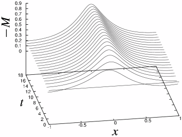
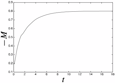
Figure 3: The left panel shows the temporal evolution of the spatial distribution of the Mach number. The right panel shows the Mach number at $x=0$.

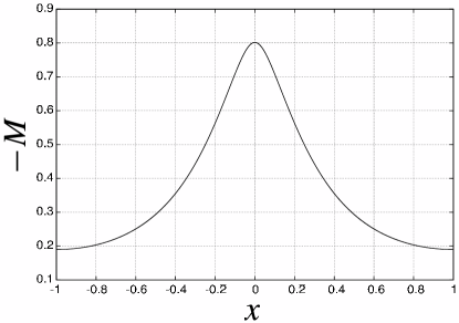
Figure 4: Spatial distribution of the Mach number at $t=18$.

The spatial distribution of the fluid velocity at $t=18$ (FIG. 4) coincides with the stationary solution (5) with $M_{\text{in}}=-0.19$ and no sonic point appears. Figure 5 shows the time derivative of the observed velocity at $x=1$ which should disappear when the fluid flow becomes stationary. Until $t\sim 4$, the initial burst mode appears, which is peculiar to our initial and boundary conditions. Then, the output signal decays exponentially. For $A_{J}\neq 0$ (with input perturbation), the output signal oscillates with a constant amplitude after the “background” flow settles down to the stationary flow.

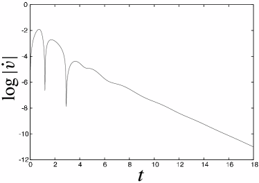
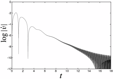
Figure 5: The temporal evolution of $\dot{v}$ at $x=1$. The left panel is $A_{J}=0$ case and the right panel is $A_{J}\neq 0$ case.

Figures 6 and 7 show the spacetime distribution of the velocity perturbation for $A_{J}\neq 0$ with $\omega_{0}=20$. In FIG. 7, to subtract the “background” flow, we have defined $\delta v=v^{(2)}-v^{(1)}$ where $v^{(i)}$ denotes the fluid velocity with the input phase $\theta_{i}$. We can see that the sound wave propagates from $x=-1$ to $x=1$. Around the throat $x=0$, the fluid velocity has larger value compared to the other region and the phase velocity of the outgoing wave becomes smaller. Thus the slope of the constant phase line becomes larger around the throat.

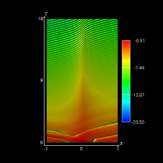
Figure 6: Spacetime distribution of $\dot{v}$ for $V_{i}=-0.19$ with $A_{J}\neq 0,\omega_{0}=20$. Colors are assigned according to the value of $\log|\dot{v}|$.

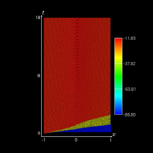
Figure 7: Spacetime distribution of the velocity perturbation $\delta v\equiv v^{(2)}-v^{(1)}$ for $V_{i}=-0.19$ with $A_{J}\neq 0,\omega_{0}=20$. Colors are assigned according to the value of $\log|\delta v|$.

Figure 8 shows the perturbation of the velocity potential at $x=1$. We set $t_{0}=3$ in Eq. (32) to obtain the velocity potential. The observed perturbation of the velocity potential oscillates with a constant amplitude.

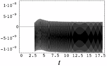
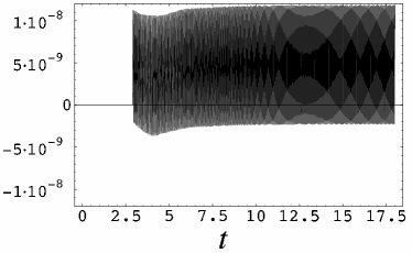
Figure 8: The temporal evolution of the velocity potential $\phi^{\text{out}(12)}$ and $\phi^{\text{out}(23)}$.

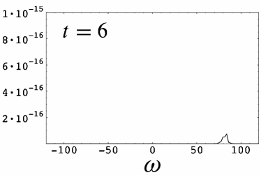
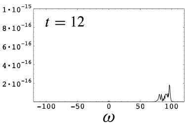
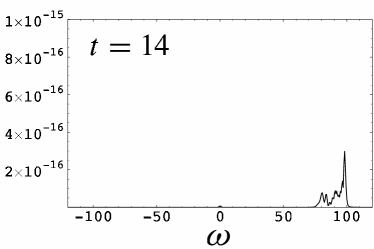
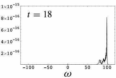
Figure 9: The temporal evolution of the power spectrum $P_{\text{obs}}(\omega)$ for the velocity potential.

The power spectrum $P_{\text{obs}}(\omega)$ obtained from the perturbations are shown in FIG. 9. The frequency of the observed signal evolves in time. This is due to the non-stationarity of the background flow as denoted by Eq. (43). Until the flow settles down to the stationary flow which is determined by the given boundary condition, the background flow evolves in time and causes the shift of the frequency of the observed perturbation. After a sufficiently long time has passed and the fluid flow becomes stationary, the observed frequency coincides with the input frequency $\omega_{0}=100$ as expected by Eq. (43).

IV.2 black hole formation case

For the initial fluid velocity $V_{i}=-0.2$, we observe the formation of the acoustic black hole. Figure 10 shows the evolution of the Mach number.

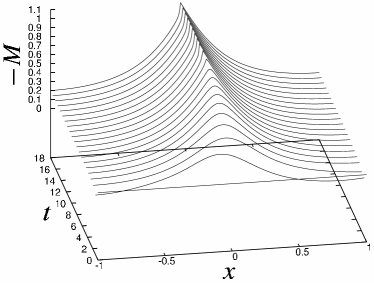
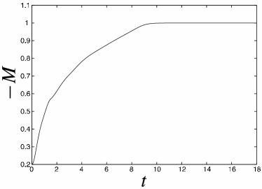
Figure 10: The left panel shows the temporal evolution of the spatial distribution of the Mach number. The right panel shows the Mach number at $x=0$.

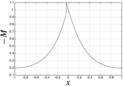
Figure 11: Spatial distribution of the Mach number at $t=18$.

At $t\sim 10$, the Mach number at the throat $x=0$ reaches unity and the sonic point appears (formation of the acoustic black hole). At the same time, the discontinuity of the derivative of the Mach number appears in the supersonic region $x<0$ as shown in FIG. 11. This discontinuity is due to the shock formed in the transonic flow. The formation of the shock is peculiar to our boundary condition which determines the Riemann invariants $J_{\pm}$ at the inlet and the outlet of the nozzle. However, since the shock occurs in the supersonic region after the formation of the sonic point, the effect of the shock never propagate into the subsonic region after the formation of the sonic point. Hence the shock never affect the sonic analogue of Hawking radiation, and we do not have to pay attention to the effect of the shock formation.

Figure 12 is the time derivative of the fluid velocity at $x=1$. After the burst mode $t\sim 4$, we can observe the quasi-normal oscillation Frolov and Novikov (1998) of the acoustic black hole with a period $\sim 4$.

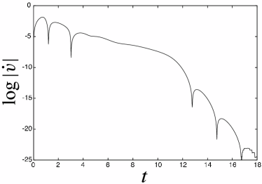
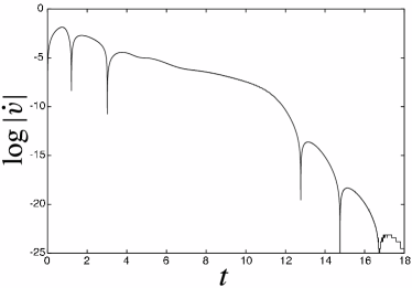
Figure 12: The temporal evolution of $\dot{v}$ at $x=1$. The left panel is $A_{J}=0$ case and the right panel is $A_{J}\neq 0$ case. As the amplitude of the input perturbation is far smaller than the change of the background, we can not see the oscillation of the perturbation in the figure (right panel).

The value of this period can be estimated as follows. In our simulation, the value of $J_{-}$ at the inlet of the nozzle is fixed to be constant by the boundary condition. Hence after the formation of the sonic horizon, the boundary condition for the ingoing perturbation $\delta J_{-}$ becomes

$$\delta J_{-}=\text{free}:\text{ at the horizon},\quad\delta J_{-}=0:\text{at the inlet of the nozzle}$$ (44)

For the outgoing perturbation $\delta J_{+}$,

$$\delta J_{+}=0:\text{ at the horizon},\quad\delta J_{+}=\text{free}:\text{ at the inlet of the nozzle}$$ (45)

By these boundary condition, a quarter of the wavelength of the quasi-normal mode is equal to a half length of the Laval nozzle and the wavelength of the quasi-normal mode becomes 4 in the present case. Thus, we obtain the period 4 of the quasi-normal mode by assuming $c_{s}=1$.

The spacetime distribution of the time derivative of the fluid velocity and the perturbation is shown in FIG. 13 and FIG. 14, respectively.

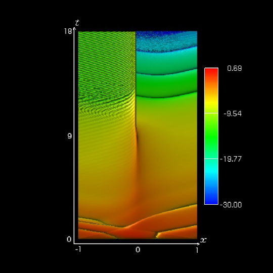
Figure 13: Spacetime distribution of $\dot{v}$ for $V_{i}=-0.2$ with $A_{J}\neq 0,\omega_{0}=20$. Colors are assigned according to the value of $\log|\dot{v}|$.

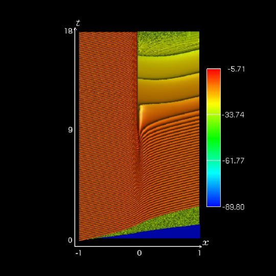
Figure 14: Spacetime distribution of the velocity perturbation $\delta v=v^{(2)}-v^{(1)}$ for $V_{i}=-0.2$ with $A_{J}\neq 0,\omega_{0}=20$. Colors are assigned according to the value of $\log|\delta v|$.

The time evolution of the observed perturbation of the velocity potential is shown in FIG. 15. After the formation of the sonic horizon $t\sim 10$, the frequency of the observed perturbation gradually decreases to zero.

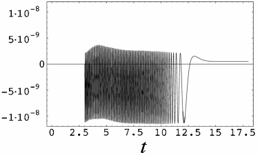
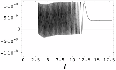
Figure 15: The temporal evolution of the velocity potential $\phi^{\text{out}(12)}$ and $\phi^{\text{out}(32)}$.

The time evolution of the power spectrum of the observed signal is shown in FIG. 16, FIG. 17 and FIG. 18. The effective frequency $\tilde{\omega}_{0}$ of the input perturbation observed at the inlet of the nozzle is $74.6$. Figure 16 shows that, after $t\sim 10$, the power spectrum of the observed perturbation spreads out toward the low $\omega$ range by the redshift effect due to the formation of the sonic horizon, and the divergence of the power $P_{\text{obs}}(\omega)$ appears at $\omega=0$. This indicates that the observed spectrum approaches the theoretically expected form (41) which diverges at $\omega=0$ as $\propto 1/\omega$. To remove this divergence, we plot $\omega^{2}P_{\text{obs}}(\omega)$ in FIG. 17 and FIG. 18.

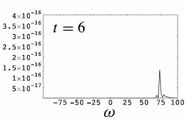
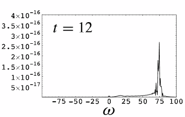
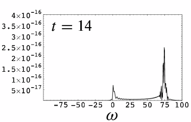
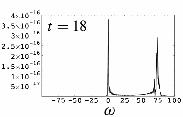
Figure 16: The temporal evolution of the power spectrum $P_{\text{obs}}(\omega)$ for the output signal.

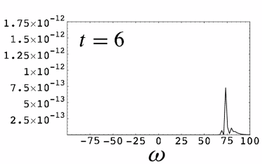
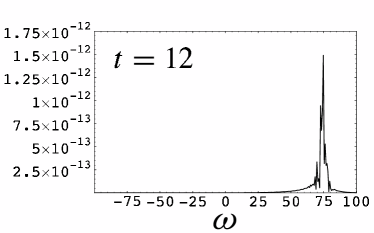
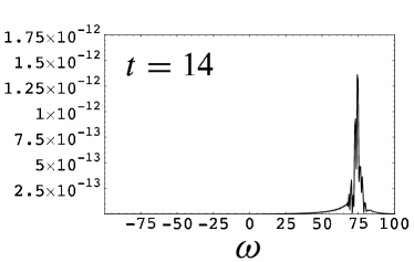
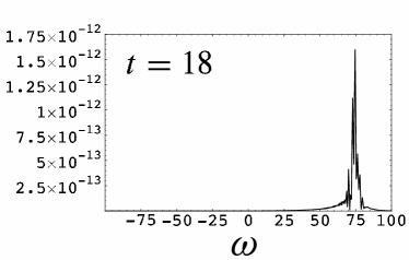
Figure 17: The temporal evolution of the power spectrum $\omega^{2}P_{\text{obs}}(\omega)$ for the output signal.

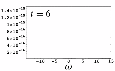
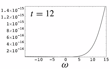
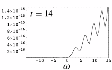
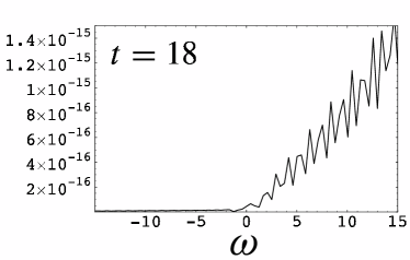
Figure 18: The temporal evolution of the power spectrum $\omega^{2}P_{\text{obs}}(\omega)$ for the output signal in the range $-15\leq\omega\leq 15$.

IV.3 Surface gravity of the sonic horizon

Figure 19 shows the observed power spectrum $\omega^{2}P_{\text{obs}}(\omega)$ at $t=18$ given by Eq. (40) and the theoretically expected power $\omega^{2}P_{\text{theory}}(\omega)$ given by Eq. (41).

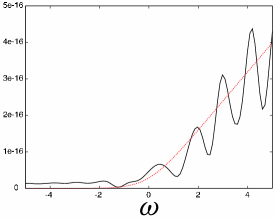
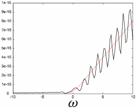
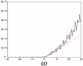
Figure 19: Power spectrums $\omega^{2}P_{\text{obs}}(\omega)$ in different ranges of $\omega$. The solid lines are the observed power spectrums and the red dotted lines are theoretically expected power (41) with $\omega_{H}=0.360$.

We fits the theoretical power spectrum to the numerical one in the range $-10\leq\omega\leq 10$ with the parameters $c_{s1}=1.00,v_{1}=-0.20,A_{J}=1.00\times 10^{-6}$ and $\tilde{\omega}_{0}=74.6$, where the value of $\tilde{\omega}_{0}$ is read off from the location of the highest peak of the power in FIG. 17. Then we obtain the surface gravity of the sonic horizon

$$\omega_{H}=\frac{\kappa_{H}}{2\pi}=0.360\pm 0.013\,.$$ (46)

This value is consistent with the theoretically expected value 0.355 given by Eq. (8).

Here we discuss about two points. The first is about the oscillation of the numerical power spectrum. This oscillation is due to the finite size Fourier transformation. This oscillation will disappear if the numerical calculation is carried out with larger value of $\omega_{0}$.

The second point is the deviation of the numerical power from the theoretical one in the high $\omega$ range. This deviation is due to the input sound wave given in the boundary condition (35). The input sound wave emerges from the outlet of the nozzle toward the inlet of the nozzle, and the observation is done at the inlet. Before the formation of the sonic point, the input sound wave comes from the outlet to the inlet without receiving a large redshift. Then, as the fluid flow evolves in time, the redshift on the observed sound wave becomes larger, and the observed frequency continues to decrease until the sonic point appears, as denoted by Eq. (43). Hence, although the input sound wave is a monochromatic wave at the outlet of the nozzle (the starting point of the propagation), the observed sound wave at the inlet of the nozzle has a broad power spectrum after the formation of the sonic point because of the stimulated effect of the redshift before the formation of the sonic point. The peak of this broad spectrum appears obviously in FIG. 17 around $\omega\sim 75$. This broadness in the power spectrum is the origin of the deviation of the numerical power from the theoretical one in FIG. 19. The perfect thermal spectrum should be realized at the infinite future, and that the theoretical power spectrum (41) is the form evaluated at the infinite future. However we have to make the observation in a finite temporal interval. Therefore, when we plot the numerical result in an appropriately large range of $\omega$, it is impossible to avoid some deviation of the numerical power from the theoretical one. If we carry out the numerical calculation longer and longer, a better agreement have to be obtained in FIG. 19.

From above discussions, we conclude that FIG. 19 shows the good agreement between the numerically obtained power and the theoretically expected form of the classical counterpart to Hawking radiation.

V Summary and conclusion

For the acoustic black hole, the classical counterpart to Hawking radiation is given by the power spectrum of the perturbation of the velocity potential of the fluid and detectable in practical experiments. To demonstrate its detectability, we performed the numerical simulation of the acoustic black hole in the Laval nozzle and observed the classical counterpart to Hawking radiation. We obtained the good agreement of the numerically observed power spectrum with the theoretically expected one.

Through our numerical simulation, we have obtained two noteworthy points for data analysis of the experiments of the acoustic black hole: the first one is that a single input wave can not give us necessary information of the classical counterpart to Hawking radiation. We need to carry out several independent observations of the sound waves with different initial phases to retrieve the thermal distribution of the power spectrum. The second one is that we can evaluate the velocity potential at the observation point by integrating the fluid velocity at that point with respect to time (see Eq. (32)). Therefore, it is not necessary to observe the sound wave at every spatial points in the fluid.

In our calculation presented here, we have considered the sound wave with small amplitude. However our numerical code is applicable beyond perturbation, in which the non-linear effect of the sound wave becomes important. By analyzing such a situation, we may be able to discuss the backreaction effect on the classical counterpart to Hawking radiation. As the next step, we are planning to extend our simulation of transonic flows in a Laval nozzle to include quantum effects. Then, we expect to obtain implications for quantum aspects of Hawking radiation using the sonic analogue model of black hole.

*

Appendix A Classical and quantum effects in Hawking radiation

We briefly review the Hawking radiation in a spacetime of a gravitational collapse forming a Schwarzschild black hole, and clarify the distinction between the quantum effects and the classical effects in the occurrence of the Hawking radiation. For simplicity, we consider a massless free scalar field $\Phi$ as a representative of the matter field, and set $c=k_{B}=1$.

For the first, we start with the classical effects. Because the spacetime is dynamical, the positive frequency modes and the negative frequency modes of the scalar field are mixed as the system evolves in time. This mixing is represented by the Bogoliubov transformation between the positive frequency mode $\phi_{\omega}$ of $\Phi$ at the past null infinity and that mode $\tilde{\phi}_{\omega}$ at the future null infinity

$$\phi_{\omega}=\int^{\infty}_{0}d\omega_{1}\left[A_{\omega\omega_{1}}\,\tilde{\phi}_{\omega_{1}}+B_{\omega\omega_{1}}\,\tilde{\phi}^{\ast}_{\omega_{1}}\,\right]\,,$$ (47)

where $\tilde{\phi}^{\ast}_{\omega}=\tilde{\phi}_{-\omega}$ is the negative frequency mode at the future null infinity. The Bogoliubov coefficients $A$ and $B$ are obtained by solving the classical wave equation $\Box\Phi=0$ with appropriate boundary conditions at the past and future null infinities and with the following relation,

$$\int_{0}^{\infty}d\omega\left[A_{\omega\omega_{1}}\,A_{\omega\omega_{2}}^{\ast}-B_{\omega\omega_{1}}\,B_{\omega\omega_{2}}^{\ast}\right]=\delta_{\omega_{1}\omega_{2}}\,,$$ (48)

which comes from the normalization condition $(\phi_{\omega_{1}},\phi_{\omega_{2}})=\delta_{\omega_{1}\omega_{2}}$ with respect to the Klein-Gordon inner product of $\Phi$ Birrell and Davis (1982). This means that the derivation of $A$ and $B$ is purely classical.

Next, in the classical framework, we consider the wave mode which propagates from the past null infinity to the future null infinity via a vicinity of the black hole horizon (see the left panel in FIG. 1). This wave mode is ingoing at the past null infinity and becomes outgoing at the future null infinity. The ingoing positive frequency mode $\phi_{\omega}$ at the past null infinity is given by

$$\phi_{\omega}(w)=\frac{1}{\sqrt{4\pi\omega}}\exp\left(-i\omega w\right),\quad\omega>0\,,$$ (49)

where $w$ is the ingoing null coordinate appropriate for the rest observer at the past null infinity. When this wave mode $\phi_{\omega}(w)$ propagates to the future null infinity via a vicinity of the horizon, it evolves to be $\phi_{\omega}(w(u))$ at the future null infinity under the geometrical optics approximation, where $u$ is the outgoing null coordinate appropriate for the rest observer at the future null infinity. The function $w(u)$ expresses the extremely large redshift which the mode $\phi_{\omega}(w)$ receives during propagating from the past null infinity to the future null infinity. This redshift effect can be decomposed into two parts: one is the redshift during the propagation from the past null infinity to the vicinity of the horizon, and the other part is the redshift after passing through the vicinity of the horizon. The first contribution is not so large and the mixing of positive and negative frequency modes does not occur. However, the second contribution is large enough to make the Bogoliubov coefficient $B_{\omega\tilde{\omega}}$ non zero. By matching the null coordinates $w$ and $u$ along a null geodesic which connects the past and future null infinities via the vicinity of the horizon, the function $w(u)$ is obtained Hawking (1975); Birrell and Davis (1982):

$$w(u)=-\alpha\exp\left(-\kappa\,u\right)+\delta,$$ (50)

where $\kappa$ is the surface gravity of the black hole horizon, $\delta$ is an arbitrary constant denoting the freedom of choosing the origin of $w$, and the constant $\alpha$ is determined by the first part of the redshift. The exponential form $\exp(-\kappa u)$ in the Eq. (50) comes from the second part of the redshift and implies that the wave length of the outgoing wave is exponentially stretched during propagating from a vicinity of the horizon to the future null infinity. That is, the wave $\phi_{\omega}(w(u))$ is no longer a pure positive frequency mode but becomes a superposition of positive and negative frequency modes at the future null infinity. In order to calculate the superposition, we need the outgoing positive frequency mode $\tilde{\phi}_{\omega}$ at the future null infinity:

$$\tilde{\phi}_{\omega}(u)=\frac{1}{\sqrt{4\pi\omega}}\,\exp\left(-i\omega\,u\right),\quad\omega>0.$$ (51)

Then, using the definition of the Bogoliubov transformation (47), the wave $\phi_{\omega}(w(u))$ at the future null infinity is decomposed as

$$\phi_{\omega}(w(u))=\int_{0}^{\infty}d\omega_{1}\left[A_{\omega\omega_{1}}\,\tilde{\phi}_{\omega_{1}}(u)+B_{\omega\omega_{1}}\,\tilde{\phi}^{\ast}_{\omega_{1}}(u)\right].$$ (52)

The Bogoliubov coefficients are obtained using the inner product $(\phi_{\omega_{1}},\tilde{\phi}_{\omega_{2}})=A_{\omega_{1}\omega_{2}}$ and $(\phi_{\omega_{1}},\tilde{\phi}^{\ast}_{\omega_{2}})=-B_{\omega_{1}\omega_{2}}$, and we find

$$\left|A_{\omega_{1}\omega_{2}}\right|^{2}=e^{\omega_{2}/\omega_{H}}\left|B_{\omega_{1}\omega_{2}}\right|^{2},\quad\left|B_{\omega_{1}\omega_{2}}\right|^{2}=\frac{1}{2\pi\kappa\omega_{1}}\frac{1}{e^{\omega_{2}/\omega_{H}}-1},\quad\omega_{H}=\frac{\kappa}{2\pi}.$$ (53)

The square of the Bogoliubov coefficients do not depend on the constants $\alpha$ and $\delta$, and the following relation holds:

$$\left|B_{\omega_{1},-\omega_{2}}\right|^{2}=\left|A_{\omega_{1}\omega_{2}}\right|^{2}\,.$$ (54)

All the above phenomena are the classical effects.

Finally we proceed to the quantum effects. When $\Phi$ is quantized, the harmonic operators $a_{\omega}$ and $a_{\omega}^{{\dagger}}$ with respect to the past mode $\phi_{\omega}$ are related to those $\tilde{a}_{\omega}$ and $\tilde{a}_{\omega}^{{\dagger}}$ with respect to the future mode $\tilde{\phi}_{\omega}$ as followsHawking (1975); Birrell and Davis (1982):

$$\tilde{a}_{\omega}=\int_{0}^{\infty}d\omega_{1}\left(A_{\omega_{1}\omega}\,a_{\omega_{1}}+B_{\omega_{1}\omega}^{\ast}\,a_{\omega_{1}}^{{\dagger}}\right),\quad\tilde{a}_{\omega}^{{\dagger}}=\int_{0}^{\infty}d\omega_{1}\left(A_{\omega_{1}\omega}^{\ast}\,a_{\omega_{1}}^{{\dagger}}+B_{\omega_{1}\omega}\,a_{\omega_{1}}\right),$$ (55)

$$[a_{\omega_{1}},a^{\dagger}_{\omega_{2}}]=\hbar\,\delta_{\omega_{1}\omega_{2}},\quad[\tilde{a}_{\omega_{1}},\tilde{a}^{\dagger}_{\omega_{2}}]=\hbar\,\delta_{\omega_{1}\omega_{2}}.$$ (56)

Then the number of particles at the future null infinity is obtained

$$N_{\omega}=\left<0\right|\tilde{a}^{{\dagger}}_{\omega}\,\tilde{a}_{\omega}\left|0\right>=\hbar\int^{\infty}_{0}d\omega_{1}\left|B_{\omega_{1}\omega}\right|^{2}\,,$$ (57)

where $\left|0\right>$ is the vacuum state at the past null infinity, $a_{\omega}\left|0\right>=0$. Therefore, for the mode $\phi_{\omega}$ which passes a vicinity of the horizon and propagates to the future null infinity, using Eqs. (53) and an appropriate regularization method Hawking (1975), we obtain

$$N_{\omega}=\left<0\right|\,\tilde{a}^{{\dagger}}_{\omega}\,\tilde{a}_{\omega}\,\left|0\right>=\frac{\hbar}{e^{\hbar\omega/\hbar\omega_{H}}-1}\,.$$ (58)

It is concluded that a black hole emits a thermal radiation of $\Phi$ with the Hawking temperature $T_{H}\equiv\hbar\,\omega_{H}$.

It should be emphasized that, although the creation of particles is just the quantum effect, however the Planckian distribution (58) of the emitted particles is purely the classical effect due to Eqs. (53). The thermal nature of the spectrum comes from the Bogoliubov coefficient $|B_{\omega_{1}\omega_{2}}|^{2}$ which has the Planckian distribution with respect to $\omega_{2}$. That is, the thermal nature of the Hawking radiation comes from the extremely large redshift for the wave mode $\phi_{\omega}$ which passes the vicinity of the horizon. If we take the classical limit $\hbar\rightarrow 0$, the number of created particles and the Hawking temperature become zero but $|B|^{2}$ is not affected.