Relic gravitational waves

in the expanding Universe

PhD Thesis of

Germán Izquierdo Sáez

to obtain the degree of

Doctor of Physics

Supervisor: Dr. Diego Pavón

Departamento de Física
(Física Estadística)
Universidad Autónoma de Barcelona
June 23, 2005

To my parents and my sister,
I owe them so many things…

Acknowledgments

This thesis had been developed during three years of quasi-full time work. I do not consider it to be “The Work of my Life” or “My Little Contribution to Human Knowledge”; but I do consider it an extremely important part of them (more than $70\%$ of the total, for sure). So many people have added to it in one way or other than I surely forgot to acknowledge someone. This is why I firstly would like to thank these ones.

Then, I thank my family, for showing so much understanding toward me; for standing up the evil Germán (whom, fortunately, no one knows very well), and for all the support they had provided me from the outset. I hope I will be able, some day, to tell them exactly what my research is about.

Next, I thank my thesis advisor, Diego, for his advise and guidance. He had transformed a recently graduated lazy student in a much-less-lazy PhD student (great effort was needed to achieve this). In these years we have shared bliss and deceptions in supporting the Real Madrid. I hope we will share fresh joys for a long period.

Time for my friends. Thanks to all my friends of the university: Dani (so many years together, so many things we have learnt, so many hilarious situations we have lived through), Jorge and Santi (two flatmates, and bad joke lovers as me), Ester (another old, old friend), Alvaro (the roommate that everybody would like to have), Vicente, Raul, Aitor, Gabriel, … Also, thanks to my friends overseas: Hong, Mariam, Jose Antonio, Andrea… And thanks to my friends beyond the academic world (for keeping me in touch with the “outside”): Agustín, Carlos, Jordi, Jose, Ricardo…

I wish to thank everybody of the Statistical Physics group of the UAB, for the good research atmosphere as well as the help they did provide me with during all these years. Especially to Javier, the first person I turned to when having a computer problem. Also, I thank the people I met at the ICG of the University of Portsmouth, for the hospitality they gave me during my two stays.

Finally, I would express my gratitude to the “Programa de Formació d’Investigadors de la UAB” for funding me for the whole period of my PhD.

And now, something completely different…

Chapter 1 Introduction

1.1 Cosmology and gravitational waves

It can be safely said that the advent of general relativity signaled the commencement of modern cosmology. The latter aims at a global description of the observable universe (i.e., the Universe). Based on observations at very large scales and some or other theory of gravitation cosmologists try to propose simple and plausible world models (i.e., models whose mathematical complexity is kept at a reasonable minimum and do not run into conflict with observational data). At present there are four main sources of observational data: the light from the faraway galaxies, whose redshifts seem to indicate that the Universe is expanding in an accelerated fashion; the abundance of light elements at cosmic scales and clusters thereof; the mass distribution of galaxies and clusters; and the anisotropies of the cosmic microwave background radiation (CMB). These are usually interpreted in favor of the $\Lambda$CDM model, a flat Friedman-Robertson-Walker universe that began expanding from an initial phase of very high density and temperature (Big Bang), and today $70\%$ of its energy would be in the form of a cosmological constant, $\Lambda$, and the rest in the form of cold (non-relativistic) matter.

The future detection of gravitational waves (GWs henceforth) is expected to provide us with invaluable information about the instant of their decoupling from other fields, i.e., about $10^{-43}$ seconds after the Big Bang. Likewise, GWs are a direct prediction of the Einstein’s field equations whence it would entail a very strong evidence in favor of general relativity. Regrettably, the weak interaction of the gravitational field with matter -that renders GWs so valuable from a cosmological viewpoint- hinders their detection.

GWs can be found originated at single sources or in a background similar to the CMB. Of the first kind are, for instance, the GWs from supernovae burst and the periodic signals from spherically asymmetric neutron stars or quark stars; of the second kind are those GWs originated at the decay of cosmic strings and the relic GWs.

This thesis is mainly concerned with relic GWs, i.e., the GWs generated by parametric amplification of the quantum vacuum during the expansion of the Universe which form a background whose spectrum depends on the scale factor. The CMB is a remnant of the radiation that once dominated the expansion of the Universe and brings us information of the decoupling between radiation and non-relativistic matter (i.e., dust). In the same way the spectrum of the relic GWs can provide us with prime information about the evolution of the scale factor, i.e., about the history of the Universe.

Even in the absence of any observed spectrum, some valuable information can be extracted from the existing bounds over it [1]. The presence of the relic GWs at the instant of the radiation–dust decoupling produces temperature fluctuations via the Sachs-Wolfe effect and, consequently, temperature anisotropies in the CMB. As these anisotriopies have been measured, a bound over the spectrum of relic GWs present at this instant follows. GWs passing by us transversely to our line of sight to a pulsar of well measured period will cause the arrival times of the pulses to shift. Many years of observation of the pulses arriving from a number of stable millisecond pulsars lead to another bound over the spectrum of the relic GWs. The theory of primordial nucleosyntesis predicts rather successfully the cosmic abundance of light elements. If at nucleosyntesis time, the contribution of relic GWs to the total energy were too large, the neutrons would have been more avaliable resulting in an overproduction of helium. These restrictions over the GWs spectrum translates into constraints on the free parameters of the universe models (see top panel of Fig. 1.1).

We assume throughout that GWs are negligibly damped by the cosmic medium; this is in keeping with common lore and well supported by different studies [2].

1.2 Gravitational waves detection

Because of insufficient technological means no direct detection of GWs has been possible so far. Nevertheless, some indirect evidences of their existence have been found. Binary systems (i.e., two stars orbiting their common center of mass) have an energy loss due to the emission of gravitational radiation that can be modelled by means of the general relativity. The observational data of the variation of the rotational period of the binary pulsar $PSR1913+16$ confirmed the predictions of the theory [3, 4]. Recently, a similar but more precise indirect proof of the existence of GWs has been obtained from the data of the variation of the orbital period of the double pulsar $J0737-3039$ [5].

The gravitational waves detection is a very topical subject and great effort is under way in that direction. There are two common types of detectors: resonant mass detectors and laser interferometers [6].

The first kind of detectors operates as the GWs produces a stress over a resonant bar (stretching or compressing it) and the vibrational amplitude or phase of the antenna experiments changes that can be measured. By making the antenna’s quadrupole modes resonant at the wave’s frequency, the detector keeps a “memory” of the excitation, allowing extra time to detect the signal. The sensitivity of this kind of antenna can be improved by increasing its mass (thus, increasing the force the GWs exert on it), by making it equally sensitive in all directions and polarizations and by lowering the thermal motion of molecules in the detector (thermal noise). Today there are seven cryogenic resonant-bar detectors in operation and three proposed resonant spheres. Analyzing the experimental results of the resonant bars EXPLORER and NAUTILUS, Astone et al. showed that the number of coincident detections is greatest when both of them are pointing into the center of our galaxy [7]. This conclusion, if not a direct detection of the GWs, can be considered a further indirect evidence of their existence.

The laser interferometer detectors use test masses which are widely separated and freely suspended (as pendulums reduce the effects of thermal noise); laser interferometry provides a means of sensing the motion of these masses produced as they interact with a gravitational wave. This technique is based on the Michelson interferometer and is particularly suited to the detection of gravitational waves as they have a quadrupole nature. Waves propagating perpendicular to the plane of the interferometer will result in one arm of the interferometer being increased in length while the other arm is decreased and vice versa. The induced change in the length of the interferometer arms results in a small change in the intensity of the light observed at the interferometer output [6]. Nowadays there are four laser interferometers taking data at their level of sensitivity: TAMA300 [8], GEO600 [9], VIRGO [10] and LIGO [11] (whose arms have a length of $300$, $600$, $3000$ and $4000$ meters, respectively).

Ground based detectors have a minimum frequency of detection bounded by seismic noise and atmospheric effects. Ground-based interferometers are also obviously limited in length to a few kilometers, restricting their coverage to events such as supernova core collapses and binary neutron star mergers. As a partial solution to these limitations, LISA - Laser Interferometer Space Antenna aimed at a launch in 2014 [12]- has been proposed by an American/European team; it consists of an array of three drag free spacecraft at the vertices of an equilateral triangle of length of side $5\times 10^{6}$ km. Proof masses inside the spacecraft (two in each spacecraft) form the end points of three separate but not independent interferometers. Each single two-arm Michelson type interferometer is formed from a vertex (actually consisting of the proof masses in a ‘central’ spacecraft), and the masses in two remote spacecraft. In the low-frequency band of LISA, sources are well known and signals are stable over long periods (many months to thousands of years). The primary sources for LISA are expected to be compact galactic binaries, supermassive black holes binaries, and extreme mass ratio inspirals. Other space based laser interferometers with a better sensitivity than LISA are being proposed: the Advanced Laser Interferometer Antenna (ALIA) and the Big Bang Observer (BBO) [13].

It is quite common, when tackling the subject of the GWs detection, to define the dimensionless parameter ${\hat{\Omega}}_{GW}(f)$ as

$${\hat{\Omega}}_{GW}(f)=f\frac{d\rho_{g}/df}{\rho_{c}},$$ (1.1)

where $f$ denotes the frequency of the wave, $\rho_{g}$ is the energy density of the GWs and $\rho_{c}=3H^{2}/(8\pi\,G)$. This parameter gives a measure of the intensity of the GWs signal and can be compared with the sensitivity of the GWs detectors (see bottom panel of Fig. 1.1).

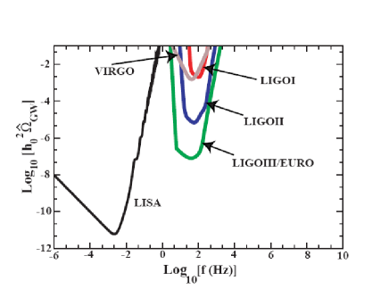
Figure 1.1: Top panel: Bounds over ${\hat{\Omega}}_{GW}$ from the CMB anisotropy (COBE), from the millisecond pulsar timing and from the Big Bang nucleosyntesis (BBN). Bottom panel: sensitivity versus frequency of LISA and ground-based detectors of first, second and third generations. The parameter $h_{0}$ is defined from $H_{0}=h_{0}\times 100km/sec/Mpc$ and represents the existing experimental uncertainty in evaluating $H_{0}$. (Adapted from Figs. 1 and 2 of Ref. [14])

1.3 Outline of the thesis

In chapter 2, we review the mechanism of amplification of the relic GWs and their power spectrum. In chapter 3, we obtain the relic GWs spectrum in a universe scenario consisting in a De Sitter stage of expansion followed by a radiation dominated stage and a dust dominated stage (three-stage model). Later, we obtain the spectrum in a four-stage model in which and additional era (dominated by a mixture of radiation and mini black holes) between the De Sitter and the radiation one. We compare both models and found bounds on the free parameters of the four-stage scenario. In chapter 4, the spectrum of GWs is obtained in a scenario with an accelerated era of expansion dominated by dark energy right after the De Sitter-radiation-dust dominated eras. Although the spectrum is formally equal to those of the three–stage model of chapter 3, it evolves differently. The possibility of the existence of a second dust era if the accelerated era comes to an end in some future time is also considered. In chapter 5, working in the De Sitter-radiation-dust-dark energy scenario and assuming the GWs entropy is proportional to the number of GWs within the event horizon (being $A$ the proportionality constant), we test the cosmological generalized second law of thermodynamics. An upper bound to the constant $A$ is found. In chapter 6, we leave the consideration of GWs to extend the study of the generalized second law of thermodynamics of the previous chapter to a universe dominated by dark energy. It turns out that the generalized second law is fulfilled in both phantom and non–phantom dark energy models provided the dark energy fluids have an entropy given by Gibbs’ equation. Finally, the Summary discusses and sum up the main results of this work. Except where otherwise stated, we use the units such that $\hbar=G=c=k_{B}=1$.

Before proceeding into the main body of the thesis it is sobering and expedient to recall the viewpoint of Willem de Sitter regarding cosmology research [15]:

“It should not be forgotten that all this talk about the Universe involves a tremendous extrapolation, which is a very dangerous operation”.

Chapter 2 The amplification mechanism of gravitational waves

2.1 The wave equation

The existence of wave-like solutions of the linearized vacuum field equations, i.e., GWs, was first predicted by Einstein in 1916 when he realized of the propagation effects inherent in the gravitational field equations [16]. The GWs equation to linear order was obtained by Lifshitz who considered perturbations that not interfered with their own propagation (as they carry little energy and momentum) [17]. He proceeded by introducing a small perturbation in the background FRW metric, $g_{ij}$,

$$\overline{g}_{ij}=g_{ij}+h_{ij}(x_{i})\qquad(i,j=0,1,2,3),$$

where $\left|h_{ij}\right|\ll\left|g_{ij}\right|$, and by evaluating the Einstein equations for the perturbation to linear order in $h_{ij}$ in a general coordinates system for which

$$h_{00}=h_{0\alpha}=0\qquad(\alpha=1,2,3).$$ (2.1)

Three kinds of solutions to the equations for the perturbation follow: scalar solutions, which represent density perturbations; vectorial solutions, which represent rotational perturbations; and tensorial solutions, which represent sourceless weak GWs.

We focus our attention on the latter kind by considering a flat FRW universe with background metric

$$ds^{2}=-dt^{2}+a(t)^{2}\left[dr^{2}+r^{2}d\Omega^{2}\right]=a(\eta)^{2}[-d\eta^{2}+dr^{2}+r^{2}d\Omega^{2}],$$ (2.2)

where $t$ and $\eta$, the cosmic and conformal time, respectively, are related through the scale factor by $a(\eta)d\eta={dt}$.

Additionally to the conditions set by equation (2.1), we impose the gauge conditions

$${h^{ij}}_{;j}=0,$$ (2.3)

where the semi-colon denotes covariant derivative with respect to the background metric (2.2). From them, it is possible to show that the perturbation has two independent components only (i.e., the wave has just two polarizations) and that the wave equation simplifies to

$${\overset{..}{{h}}_{\alpha}}^{\beta}+3\frac{\overset{.}{a}}{a}{\overset{.}{{h}}_{\alpha}}^{\beta}+g^{\gamma\delta}{{h_{\alpha}}^{\beta}}_{,\gamma,\delta}=0,$$ (2.4)

where the upper dot and the commas indicate partial derivatives respect to time and spatial coordinates, respectively.

Introducing the ansatz

$${h_{\alpha}}^{\beta}(t,\textbf{x})=h(t){G_{\alpha}}^{\beta}(\textbf{k},\textbf{x}),$$ (2.5)

where ${G_{\alpha}}^{\beta}$ is a combination of plane-waves solutions $exp(\pm i\textbf{k}\textbf{x})$ that contain the two polarizations of the wave mentioned above and fulfill

$${G_{\alpha}^{\beta}}^{;\gamma}_{;\gamma}=-k^{2}G_{\alpha}^{\beta},\qquad{G^{\beta}_{\alpha}}_{;\beta}=G^{\alpha}_{\alpha}=0,$$ (2.6)

into equation (2.4) leads to the evolution equation for the temporal part of the wave

$${\overset{..}{h}}(k,t)+3\frac{\overset{.}{a}}{a}{\overset{.}{h}(k,t)}+\frac{k^{2}}{a^{2}}{h}(k,t)=0.$$ (2.7)

Or, in terms of the conformal time

$$h^{\prime\prime}(k,\eta)+2\frac{a^{\prime}}{a}h^{\prime}(k,\eta)+k^{2}h(k,\eta)=0,$$ (2.8)

where the prime indicates derivative with respect to $\eta$.

In the equations of above we have used the comoving wave-number $k=|\textbf{k}|$, which is related with the wave-length and the frequency of the wave by

$$k=\frac{2\pi a}{\lambda}=a\omega.$$ (2.9)

Equation (2.8) can be suitably simplified by using the ansatz $h(k,\eta)=\mu(k,\eta)/a(\eta)$. This yields the so called Lifshitz’s equation

$$\mu^{\prime\prime}(\eta)+\left(k^{2}-\frac{a^{\prime\prime}(\eta)}{a(\eta)}\right)\mu(\eta)=0.$$ (2.10)

It parallels the time independent Schrödinger equation where the terms $k^{2}$ and $a^{\prime\prime}/a$ play the role of the energy and the potential, respectively. It can be also interpreted as the equation of an harmonic oscillator parametrically excited by the term $a^{\prime\prime}/a$. When $k^{2}\gg\frac{a^{\prime\prime}}{a}$, i.e., for high frequency waves, expression (2.10) becomes the equation of an harmonic oscillator whose solution is a free wave, and consequently the amplitude of $h_{\alpha\beta}(\eta,\mathbf{x})$ decreases adiabatically as $a^{-1}$ in an expanding universe. In the opposite regime, $k^{2}\ll\frac{a^{\prime\prime}}{a}$, the general solution to (2.10) is a linear combination of the pair of solutions

$$\mu_{1}=a(\eta),{\qquad}{\qquad}\mu_{2}=a(\eta)\int d\eta\ a^{-2}(\eta).$$ (2.11)

If the universe is expanding, $\mu_{1}$ will grow faster than $\mu_{2}$ and will soon dominate. In this case, the amplitude of $h_{\alpha\beta}(\eta,\mathbf{x})$ will remain constant as long as $k^{2}\ll\frac{a^{\prime\prime}}{a}$. If at some future time this condition is no longer satisfied, the wave will have an amplitude larger than it would in accordance with the adiabatic behavior. This phenomenon is called “superadiabatic” or “parametric” amplification of gravitational waves [18].

GWs that fulfill the condition $k^{2}\ll a^{\prime\prime}/a$ ($k^{2}\gg a^{\prime\prime}/a$) are considered to be well inside (outside) of the Hubble radius [19], i.e., their wave lengths are shorter (longer) than $\lambda_{H}=H^{-1}(\eta)$, where $H=a^{\prime}/a^{2}$ is the Hubble function, and

$$k<2\pi aH(\eta)\qquad\left(k>2\pi aH(\eta)\right).$$ (2.12)

This can be traced to the fact that the ratio between $(2\pi aH(\eta))^{2}$ and the term $a^{\prime\prime}/a$ is always constant for a perfect fluid with an equation of state of barotropic type, $p=(\gamma-1)\rho$, and tends to zero as soon as $\gamma\rightarrow 4/3$.

2.2 Gravitational waves creation

In the previous subsection we have seen how the GWs may undergo “parametric” amplification. This approach is based on the idea that the amplitude of each GW is enlarged during the expansion of the universe. Usually the initial amplitude is assumed to be the vacuum one, $A(k)\sim k$ [20]. The rationale behind this is the following. One assimilates the quantum zero-point fluctuations of vacuum with classical waves of certain amplitudes and arbitrary phases; consequently it is permissible to equalize $\omega/2$ with the energy density of the gravitational waves, $h^{2}/\lambda^{2}$ times $\lambda^{3}$. Thereby the initial vacuum amplitude of GWs is given by $h\propto A(k)\propto k$ [18].

A different approach can be developed by realizing that Lifshitz’s equation (2.10) is not invariant under conformal transformations of the metric [21, 22]

$$g_{ij}\rightarrow\widehat{g}_{ij}=\Omega^{2}(t,\textbf{x})g_{ij},$$ (2.13)

where $\Omega^{2}(t,\textbf{x})$ is a real, continuous, finite and non vanishing function, except when $a^{\prime\prime}=0$. With this in mind, the “parametric” amplification may be interpreted as spontaneous GWs creation due to the action of the expansion of the Universe over the initial vacuum.

2.2.1 A simple example: the quantum pendulum

The ideal pendulum, a weight hanging from a string of length $l$, pedagogically illustrates the phenomena of particle creation from the initial vacuum. The pendulum oscillates around its equilibrium position with frequency $\sqrt{g/l}$. If the string is wound around a reel, the length of the string can vary as well as the oscillation frequency.

Being the pendulum initially at the minimum energy configuration, we increase the length of the string by lowering the bob, in a time interval $\tau=t_{f}-t_{i}$, from an initial value $l_{i}$ to a final value $l_{f}$. Classically, the pendulum (initially at rest) will be also at rest in the final state and the change of potential energy will equal the friction work.

From a quantum mechanic point of view, the initial minimum energy configuration of the system corresponds to the state with energy $E_{i}=\omega_{i}/2$ and number of quanta $N_{i}=0$. If the time spent in lowering the bob is much longer than the initial and final periods of oscillation, i.e., $\tau\gg T_{f}=2\pi/\omega_{f}$ (the adiabatic case), the bob undergoes more than one complete oscillation during the process. In this case the final energy is $E_{f}=\omega_{f}/2$ and the number of quanta in the final state is $N_{f}=0$. The potential energy obtained is partly dissipated by the reel, as in the classical approach, but also by the change of the energy from the initial to the final state.

By contrast, if the time spent in lowering the bob is much shorter than the initial and final periods of oscillation, i.e., $\tau\ll T_{i}=2\pi/\omega_{i}$, things fare differently. The final energy of the oscillator will be half the energy of the initial state $E_{f}=E_{i}/2$ and the final vacuum energy will be $\omega_{f}/2$ (see Ref [1] for details). Consequently, the final number of quanta $N_{f}=\frac{1}{4}\frac{\omega_{i}}{\omega_{f}}$ will differ from zero. Note that these quanta are created because of the sudden change in the vacuum state.

In the case of the GWs, we must replace the pendulum equation for equation (2.10). The role of the variable length $l$ is now played by the term $a^{\prime\prime}(\eta)/a(\eta)$. If $a^{\prime\prime}(\eta)/a(\eta)$ varies slowly compared with the wave number $k$, the initial vacuum state will evolve into the final vacuum state and no GW will be generated. But if $a^{\prime\prime}(\eta)/a(\eta)$ evolves fast enough, the final state will not be the vacuum one and GWs will be spontaneously generated.

2.2.2 Bogoliubov coefficients

In Minkowski spacetime, a scalar field $\phi$ of mass $m$ obeys the Klein-Gordon equation

$$\left(\eta^{ij}\partial_{i}\partial_{j}+m^{2}\right)\phi=0,$$ (2.14)

where $\eta^{ij}$ represents the metric. The field $\phi$ can be expanded as

$$\phi(x)=\sum_{\mathbf{k}}[A_{\mathbf{k}}\nu_{\mathbf{k}}(x)+A_{\mathbf{k}}^{\dagger}\nu_{\mathbf{k}}^{\ast}(x)],{\ }$$ (2.15)

in terms of the family of modes

$$\nu_{\mathbf{k}}=\frac{1}{4\pi\sqrt{\pi k}}\,e^{i(\mathbf{k\cdot x}-kt)},$$ (2.16)

which are positive-frequency defined with respect to $t$

$$\frac{\partial\nu_{\mathbf{k}}}{\partial t}=-ik\nu_{\mathbf{k}}{\qquad}(k>0).$$ (2.17)

This set of modes forms a privileged family: it defines creation and annihilation operators $A_{\mathbf{k}}$ and $A_{\mathbf{k}}^{\dagger}$, respectively, representing real particles for all inertial observers, as the quantum vacuum defined by the modes is invariant under Poincaré transformations.

In curved spacetime, the equation obeyed by the scalar field reads

$$g^{ij}\phi_{;i;j}+\left(m^{2}+\xi R\right)\phi=0$$ (2.18)

where $\xi$ is a dimensionless parameter and $R$ is the Ricci scalar. The term $\xi R$ accounts for the coupling between the scalar and the gravitational field.

When $m=0$ and $\xi=1/6$, equation (2.18) is conformally invariant. In this case if the spacetime considered can be transformed conformally in the Minkowski one, it is possible to define a new field that obeys equation (2.14) and privileged modes can be chosen in order to define a vacuum state. However, generally, there is no privileged family of modes as the Poincaré group is no longer a symmetry.

In general, given a complete collection of modes $\nu_{m}(x)$ the field can be expanded as

$$\phi(x)=\sum_{m}[A_{m}\nu_{m}(x)+A_{m}^{\dagger}\nu_{m}^{\ast}(x)],{\ }$$ (2.19)

where $A_{m}$ and $A_{m}^{\dagger}$ are, respectively, the annihilation and creation operators associated to the quantum vacuum state of the family, $|0\rangle$. The field can also be expanded as

$$\phi(x)=\sum_{n}\left[\overline{A}_{n}\overline{\nu}_{n}(x)+\overline{A}_{n}^{\dagger}\overline{\nu}_{n}^{\ast}(x)\right],$$ (2.20)

in terms of a different complete collection of modes, $\overline{\nu}_{n}(x)$, with a different vacuum state, $|\overline{0}\rangle$.

The Bogoliubov transformation

$$\overline{\nu}_{n}(x)=\sum_{m}\left[\alpha_{nm}\nu_{m}(x)+\beta_{nm}\nu_{m}^{\ast}(x)\right],$$ (2.21)

where $\alpha_{nm}$ and $\beta_{nm}$ are the coefficients of Bogoliubov, relates both families of modes. From equations (2.19)-(2.21), it is readily seen that

$$A_{m} = \sum_{n}(\alpha_{nm}\overline{A}_{n}+\beta_{nm}\overline{A}_{n}^{\dagger}),$$ (2.22)

$$\overline{A}_{n} = \sum_{m}(\alpha_{nm}A_{m}+\beta_{nm}A_{m}^{\dagger}).$$ (2.23)

As the creation/annihilation operators satisfy the commutation relation $[A_{m},A_{m}^{\dagger}]=[\overline{A}_{n},\overline{A}_{n}^{\dagger}]=1$, the Bogoliubov coefficients must fulfill

$$|\alpha_{nm}|^{2}-|\beta_{nm}|^{2}=1.$$ (2.24)

The operator number of particles of the first family, $N_{m}=A_{m}^{\dagger}A_{m}$, acts upon the quantum vacuum state of the second family according to

$$\langle\overline{0}|N_{m}|\overline{0}\rangle=\langle\overline{0}|A_{m}^{\dagger}A_{m}|\overline{0}\rangle=\sum_{n}|\beta_{nm}|^{2}.$$ (2.25)

Therefore, the quantum vacuum state of the second family contains $\sum_{n}|\beta_{nm}|^{2}$ particles of the first family. An entirely similar relation holds for the first family vacuum state and the second family number of particles operator.

The GWs equation (2.8) formally coincides with the equation of a massless decoupled field in a spatially flat FRW spacetime. Its solutions are

$$h_{ij}(\eta,\mathbf{x})=\int\left(A_{(k)}h_{ij}^{(k)}(\mathbf{k},x)+A_{(k)}^{\dagger}{h_{ij}^{(k)}}^{*}(\mathbf{k},x)\right)d^{3}k.$$ (2.26)

The modes $h_{ij}^{(k)}(\mathbf{k},x)$ can be written as

$$h_{ij}^{(k)}(\mathbf{k},x)=\frac{\sqrt{8\pi}}{(2\pi)^{3/2}}e_{ij}(\mathbf{k})\frac{\mu_{(k)}(\eta)}{a(\eta)}e^{i\mathbf{k\cdot x}}\mathbf{,}$$ (2.27)

where $e_{ij}(\mathbf{k})$ contains both polarizations of the wave, and the functions $\mu_{(k)}(\eta)$ are solutions to (2.10). As the family of modes that quantify the field is complete, the modes $h_{ij}^{(k)}(\mathbf{k},x)$ must be orthogonal, i.e.,

$$-i\int\left(h_{ij}^{(k)}(\mathbf{k},x){h_{ij}^{(k^{\prime})}}^{*\prime}(\mathbf{k},x)-{h_{ij}^{(k)}}^{\prime}(\mathbf{k},x){h_{ij}^{(k^{\prime})}}^{*}(\mathbf{k},x)\right)d^{n-1}x=\delta(\mathbf{k}-\mathbf{k}^{\prime}),$$ (2.28)

and, therefore, $\mu_{(k)}$ obeys the further condition

$$\mu_{(k)}\mu^{*\prime}_{(k)}-\mu_{(k)}^{*}\mu_{(k)}^{\prime}=i.$$ (2.29)

If the spatially flat FRW universe contains a perfect fluid with equation of state

$$p=(\gamma-1)\rho,$$ (2.30)

with $\gamma$ constant, the Einstein equations

$$\left(\frac{a^{\prime}}{a^{2}}\right)^{2}=\frac{8\pi}{3}\rho,$$ (2.31)

$$\rho^{\prime}+3\frac{a^{\prime}}{a}(\rho+p)=0,$$ (2.32)

can be solved to

$$a(\eta)=a_{i}\left(\frac{a_{i}H_{i}}{l}\right)^{l}\left(\eta-\eta_{i}+\frac{l}{a_{i}H_{i}}\right)^{l},$$ (2.33)

where $a_{i}$, $H_{i}$ and $\eta_{i}$ are, respectively, the initial values of the scale factor, the Hubble function and the conformal time and $l=2/(3\gamma-2)$. For simplicity, we define $\eta_{l}=\eta-\eta_{i}+l/(a_{i}H_{i})$ and Lifshitz’s equation reduces to the Bessel equation

$$\mu^{\prime\prime}(\eta)+\left[k^{2}-\frac{l(l-1)}{(\eta_{l})^{2}}\right]\mu(\eta)=0,$$ (2.34)

whose solutions can be written in terms of Hankel functions as

$$\mu_{l}(\eta)=\frac{\sqrt{\pi}}{2}k^{-1/2}x_{l}^{1/2}\left[D_{1l}H_{l-\frac{1}{2}}^{(1)}(x_{l})+D_{2l}H_{l-\frac{1}{2}}^{(2)}(x_{l})\right],$$ (2.35)

where $x_{l}=k\eta_{l}$, and $D_{1l}$ and $D_{2l}$ are integration constants.

Henceforward, we shall work in the Heisenberg picture, the quantum states are functions of time meanwhile the operators are time independent. Initially the universe will be in some state from which the number of GWs operator will be defined. As the scale factor evolves, the quantum state evolves too and the constant operator acts upon this state which is no longer the initial one.

In this scenario, it seems problematic to choose the appropriate vacuum state or to define real particles. A possible solution to this problem rests on the concept of adiabatic vacuum.

2.2.3 The adiabatic vacuum approximation

This approximation rests on the idea that the creation of particles by a slow change in the initial state is minimal [22].

Solutions to the equation

$$\chi^{\prime\prime}+\omega^{2}(\eta)\chi=0,$$ (2.36)

with $\omega\in C^{\infty}$ are expressed as a linear combination of basis functions which can be approximated by

$$\chi^{\pm}(\eta)=\frac{1}{\sqrt{2W(\eta)}}\exp\left(\mp i\int^{\eta}W(\eta^{\prime})d\eta^{\prime}\right)+\mathcal{O}(\omega^{-N}),$$ (2.37)

with

$$W^{2}(\eta)=\omega^{2}(\eta)\left[1+\chi_{2}(\eta)\omega^{-2}+\chi_{4}(\eta)\omega^{-4}+...\right],$$ (2.38)

where the $\chi_{n}(\eta)$ are functions of $\omega(\eta)$ and its derivatives up to the derivative of order $n$, which is bounded as $\omega\rightarrow\infty$ [23]. If we introduce the adiabatic parameter $\Theta$ by replacing $\Theta\,\omega(\eta)$ for $\omega(\eta)$ (at the end we can let $\Theta=1$), the adiabatic behavior (slow expansion limit) of equation (2.36) can be examined when $\Theta\rightarrow\infty$, and, in this limit, the above expression can be considered a power-series expansion in $\Theta^{-1}$ to order $N$.

Equations (2.10) and (2.36) share the same form. Thus, we can define the adiabatic vacuum of order $N$ by taking $\mu$ in equation (2.27) as an exact solution to (2.10) whose WKB approximation is precisely $\chi^{+}$ in (2.37). To this order, the operators $A_{(k)}$ in (2.26) correspond exactly to physical particles when $\Theta\rightarrow\infty$ or when $k\rightarrow\infty$.

Note that in this limit, the modes $h_{ij}^{(k)}$ tend to the positive-frequency Minkowski modes. Hence, the constants in equation (2.35) turn out to be $D_{1l}=0$ and $D_{2l}=1$, thereby

$$\mu_{l}=(\sqrt{\pi}/2)e^{i\psi_{l}}k^{-1/2}x_{l}^{1/2}H_{l-\frac{1}{2}}^{(2)}(x_{l}).$$ (2.39)

2.2.4 The creation mechanism

Let us assume that the spatially flat FRW universe considered above goes through a succession of stages, and that, in a generic stage $r$, the Universe is dominated by a perfect fluid of barotropic index $\gamma_{r}$. The transitions between the different stages can be considered instantaneous or, more accurately, much shorter than the duration of each stage.

The scale factor, in this scenario, is given by equation (2.33) with a different $l_{r}$ in each era and the subindex $i$ denoting the beginning of the $r$-stage (i.e., the end of the ($r-1$)-stage). Note that the scale factor must be continuous at each transition $\eta_{i}$ as no discontinuities must be present in the FRW metric. In each stage the solution to Lifshitz’s equation (2.10) is (2.39) with $l$ replaced by $l_{r}$.

The modes of two consecutive stages (namely the ($r-1$)-stage and the $r$-stage) are related by a Bogoliubov transformation

$$\mu_{l_{r-1}}(\eta_{i})=\alpha_{i}\mu_{l_{r}}(\eta_{i})+\beta_{i}\mu_{l_{r}}^{\ast}(\eta_{i}).$$ (2.40)

Since the functions $\mu_{l_{r}}(\eta)$ and $\mu^{\prime}_{l_{r}}(\eta)$ must be also continuous at $\eta_{i}$ (further details about the continuity of $\mu$ and the validity of the sudden transition approximation are given in the Appendix), it is possible to obtain the expression of the Bogoliubov coefficients in terms of known quantities [24, 25]

$$\alpha_{i}=i[\mu_{l_{r-1}}^{\prime}(\eta_{i})\mu_{l_{r}}^{*}(\eta_{i})-\mu_{l_{r-1}}(\eta_{i}){\mu_{l_{r}}^{*}}^{\prime}(\eta_{i})],$$ (2.41)

$$\beta_{i}=i[\mu_{l_{r-1}}(\eta_{i})\mu_{l_{r}}^{\prime}(\eta_{i})-\mu_{l_{r-1}}^{\prime}(\eta_{i})\mu_{l_{r}}(\eta_{i})].$$ (2.42)

The adiabatic approximation sets a bound over the GWs that can be created in this transition. The limit of slow expansion, $\omega\rightarrow\infty$, can be relaxed by assuming that there is no creation of waves for $\omega(\eta_{i})\gg\omega_{i}$. This bound can be fixed as the frequency associated to the characteristic time in which takes place the transition. Modes whose period at the instant $\eta_{i}$ are shorter than this transition time experiment an adiabatic expansion thereby they still represent the quantum vacuum state, i.e., for them, $\alpha_{i}=1$ and $\beta_{i}=0$. Meanwhile modes whose period at the transition $\eta_{i}$ is larger than this characteristic time do not represent the quantum vacuum state any longer, and $\beta_{i}\neq 0$. This characteristic time is usually chosen as the inverse of the Hubble parameter at the transition, $H_{i}^{-1}$. Then, the adiabatic bound for the frequencies at $\eta>\eta_{i}$ reads

$$\omega_{i}(\eta)=2\pi\frac{a_{i}}{a(\eta)}H_{i},$$ (2.43)

where we have taken into account the redshift.

Assuming that each created GW has an energy $2\,\omega(\eta)$ (the factor $2$ comes from the two polarization states), it is possible to express the energy density of GWs created at the transition $\eta_{i}$ with frequencies in the range $\left[\omega(\eta),\omega(\eta)+d\omega(\eta)\right]$ as

$$d\rho_{g}(\eta)=2\omega(\eta)\left[\frac{\omega^{2}(\eta)}{2\pi^{2}}d\omega(\eta)\right]|\beta_{i}|^{2}=P(\omega(\eta))d\omega(\eta),$$ (2.44)

where $P(\omega(\eta))=\left(\omega^{3}(\eta)/\pi^{2}\right)|\beta_{i}|^{2}$ denotes the power spectrum. As the energy density is a locally defined quantity, $\rho_{g}$ loses its meaning for metric perturbations whose wave length $\lambda=2\pi/\omega(\eta)$ exceed the Hubble radius $H^{-1}(\eta)$. Integrating over the frequency, we get the total energy density

$$\rho_{g}(\eta)=\int^{\omega_{i}(\eta)}_{2\pi H(\eta)}P(\omega(\eta))d\omega(\eta).$$ (2.45)

The adiabatic cutoff amounts to a renormalization of the quantum field theory. This upper bound ensures that the energy density does not diverge at high frequencies. The adiabatic bound plays the same role that the extraction of the energy of the vacuum in the quantum field theories in Minkowski spacetime.

To relate the $\mu_{l}$ functions of two non-consecutive stages, we must make use of the total Bogoliubov coefficients which can be found recursively from

$$\alpha_{T_{i}}=\alpha_{i}\alpha_{T_{(i-1)}}+\beta_{i}^{\ast}\beta_{T_{(i-1)}},$$ (2.46)

$$\beta_{T_{i}}=\beta_{i}\alpha_{T_{(i-1)}}+\alpha_{i}^{*}\beta_{T_{(i-1)}},$$ (2.47)

where the subindex $(i-1)$ denotes the previous transition to the $i$-th one [24].

Equations (2.46) and (2.47) readily follow from the Bogoliubov transformation

$$\left(\begin{array}[]{l}\mu_{l_{r-1}}\\ \mu_{l_{r-1}}^{\ast}\end{array}\right)=\left(\begin{array}[]{ll}\alpha_{i}&\beta_{i}\\ \beta_{i}^{\ast}&\alpha_{i}^{\ast}\end{array}\right)\left(\begin{array}[]{l}\mu_{l_{r}}\\ \mu_{l_{r}}^{\ast}\end{array}\right).$$ (2.48)

Thus, the modes of the $r-n$ stage, $\mu_{l_{r-n}}$, are related with $\mu_{l_{r}}$

$$\left(\begin{array}[]{l}\mu_{l_{r-n}}\\ \mu_{l_{r-n}}^{*}\end{array}\right)=\left(\begin{array}[]{ll}\alpha_{i-(n-1)}&\beta_{i-(n-1)}\\ \beta_{i-(n-1)}^{*}&\alpha_{i-(n-1)}^{*}\end{array}\right)...\left(\begin{array}[]{ll}\alpha_{i-1}&\beta_{i-1}\\ \beta_{i-1}^{*}&\alpha_{i-1}^{*}\end{array}\right)\left(\begin{array}[]{ll}\alpha_{i}&\beta_{i}\\ \beta_{i}^{*}&\alpha_{i}^{*}\end{array}\right)\left(\begin{array}[]{l}\mu_{l_{r}}\\ \mu_{l_{r}}^{*}\end{array}\right),$$ (2.49)

(note there is $n-1$ transitions between both eras). After simplifying we get

$$\left(\begin{array}[]{l}\mu_{l_{r-n}}\\ \mu_{l_{r-n}}^{*}\end{array}\right)=\left(\begin{array}[]{ll}\alpha_{T_{i}}&\beta_{T_{i}}\\ \beta_{T_{i}}^{*}&\alpha_{T_{i}}^{*}\end{array}\right)\left(\begin{array}[]{l}\mu_{l_{r}}\\ \mu_{l_{r}}^{*}\end{array}\right).$$ (2.50)

We will employ Eqs. (2.46) and (2.47) in the following chapters.

Chapter 3 Quantum mini black holes and the gravitational waves spectrum

In this chapter we consider in detail the power spectrum of relic GWs assuming the Universe went through an expansion era dominated by radiation and mini black holes (MBHs) intermediate between the conventional inflationary (De Sitter) era and the radiation dominated era [26]. The existence of that era is justified in subsection 3.2. In subsection 3.1 we recall the derivation of the power spectrum of the conventional three-stage scenario.

3.1 Three-stage spatially flat FRW scenario

Here we apply the fundamental equations found in the previous chapter to a spatially flat FRW scenario consisting in an initial De Sitter stage, followed by a radiation dominated era and a dust era that includes the present time. The power spectrum predicted for this scenario is well known in the literature, see Refs. [24] and [27]-[29]. The scale factor is given by

$$a(\eta)=\left\{\begin{array}[]{c}-\frac{1}{H_{1}\eta}\qquad(-\infty<\eta<\eta_{1}<0),\\ \frac{1}{H_{1}\eta_{1}^{2}}(\eta-2\eta_{1})\qquad(\eta_{1}<\eta<\eta_{2}),\\ \frac{1}{4H_{1}\eta_{1}^{2}}\frac{(\eta+\eta_{2}-4\eta_{1})^{2}}{\eta_{2}-2\eta_{1}}{\qquad}(\eta_{2}<\eta<\eta_{0}).\end{array}\right.$$ (3.1)

The initial state is the vacuum associated with the modes of the inflationary stage $\mu_{I}(\eta)$, which are a solution to Lifshitz’s equation (2.10) compatible with the condition (2.29). Taking into account that $l=-1$ in this era (De Sitter), the modes read

$$\mu_{I}=(\sqrt{\pi}/2)e^{i\psi_{I}}k^{-1/2}x^{1/2}H_{-3/2}^{(2)}(x),$$ (3.2)

where $x=k\eta$, $\psi_{I}$ is an arbitrary constant phase and $H_{-3/2}^{(2)}(x)$ is the Hankel function of order $-3/2$. The proper modes of the radiation era ($l=1$) are

$$\mu_{R}=(\sqrt{\pi}/2)e^{i\psi_{R}}k^{-1/2}x_{R}^{1/2}H_{1/2}^{(2)}(x_{R}),$$ (3.3)

where $x_{R}=k(\eta-2\eta_{1})$ and $\psi_{R}$ is again a constant phase.

The “parametric” amplification in this first transition was first developed by Grishchuk [21] and Starobinsky [29]. Following the quantum approach, the two families of modes are related by

$$\mu_{I}(\eta)=\alpha_{1}\mu_{R}(\eta)+\beta_{1}\mu_{R}^{\ast}(\eta).$$ (3.4)

From equations (2.41) and (2.42), we obtain

$$\alpha_{1}=-1+\frac{i}{k\eta_{1}}+\frac{1}{2(k\eta_{1})^{2}},\qquad\beta_{1}=\frac{1}{2(k\eta_{1})^{2}},$$ (3.5)

where we have neglected an irrelevant phase. Considering the adiabatic quantum approximation, the modes whose frequency at the transition are larger than the characteristic time scale ($H_{1}^{-1}$) get exponentially suppressed. Thus, the coefficients are $\alpha_{1}=1$ and $\beta_{1}=0$ for GWs with $k>2\pi a_{1}H_{1}$ and (3.5) when $k<2\pi a_{1}H_{1}$.

In the dust era ($\eta>\eta_{2}$ and $l=2$) the solution for the modes is

$$\mu_{D}=(\sqrt{\pi}/2)e^{i\psi_{D}}k^{-1/2}x_{D}^{1/2}H_{3/2}^{(2)}(x_{D}),$$ (3.6)

where $x_{D}=k\left(\eta+\eta_{2}-4\eta_{1}\right)$ and it is related to the radiation ones by

$$\mu_{R}(\eta)=\alpha_{2}\mu_{D}(\eta)+\beta_{2}\mu_{D}^{\ast}(\eta).$$ (3.7)

Similarly one obtains

$$\alpha_{2}=-i\left(1+\frac{i}{2k(\eta_{2}-2\eta_{1})}-\frac{1}{8\left(k(\eta_{2}-2\eta_{1})\right)^{2}}\right),\qquad\beta_{2}=\frac{i}{8\left(k(\eta_{2}-2\eta_{1})\right)^{2}},$$ (3.8)

for $k<2\pi a(\eta_{2})H_{2}$ and $\alpha_{2}=1$, $\beta_{2}=0$ for $k>2\pi a(\eta_{2})H_{2}$ where $H_{2}$ is the Hubble function evaluated at the radiation-matter transition $\eta_{2}$.

In order to relate the modes of the inflationary era to the modes of the dust era, we make use of the total Bogoliubov coefficients $\alpha_{Tr2}$ and $\beta_{Tr2}$, given by equations (2.46) and (2.47). For $k>2\pi a_{1}H_{1}$, we find that $\alpha_{Tr2}=1$ and $\beta_{Tr2}=0$; in the range $2\pi a_{1}H_{1}>k>2\pi a_{2}H_{2}$, the coefficients are $\alpha_{Tr2}=\alpha_{1}$ and $\beta_{Tr2}=\beta_{1}$, and finally for $k<2\pi a(\eta_{2})H_{2}$ we obtain that

$$\beta_{Tr2}\simeq-\frac{2(\eta_{2}-2\eta_{1})+\eta_{1}}{8k^{3}\eta_{1}^{2}(\eta_{2}-2\eta_{1})^{2}}.$$ (3.9)

Thus the number of GWs at the present time, $\eta_{0}$, created from the initial vacuum state is $\left\langle N_{\omega}\right\rangle=\left|\beta_{Tr2}\right|^{2}\sim\omega^{-6}(\eta_{0})$ for $\omega(\eta_{0})<2\pi(a_{2}/a_{0})H_{2}$, $\omega^{-4}(\eta_{0})$ for $2\pi(a_{1}/a_{0})H_{1}>\omega(\eta_{0})>2\pi(a_{2}/a_{0})H_{2}$ and zero for $\omega(\eta_{0})>2\pi(a_{1}/a_{0})H_{1}$, where we have used the present value of the frequency, $\omega(\eta_{0})=k/a_{0}$.

The present power spectrum of GWs predicted by this model is

$$P\left(\omega\right)\sim\left\{\begin{array}[]{ll}0&\left(\omega(\eta_{0})>2\pi(a_{1}/a_{0})H_{1}\right),\\ \omega^{-1}(\eta_{0})&\left(2\pi(a_{2}/a_{0})H_{2}<\omega(\eta_{0})<2\pi(a_{1}/a_{0})H_{1}\right),\\ \omega^{-3}(\eta_{0})&\left(2\pi H_{0}<\omega(\eta_{0})<2\pi(a_{2}/a_{0})H_{2}\right).\end{array}\right.$$ (3.10)

The spectrum (3.10) is shown in figure 3.1 tagged as $l=1$ for different choices of $H_{1}$, $a_{1}/a_{0}$ and $a_{2}/a_{0}$.

Below we compare the predictions of the three-stage model of above, for the frequency ranges and powers, with the four-stage model that includes the “MBHs+rad” era.

3.2 GWs in a FRW universe with an era of mini black holes and radiation

3.2.1 Mini black holes in the very early Universe

As is well known, MBHs can be created by quantum tunnelling from the hot radiation with a rate of nucleation given by [30]

$$\Gamma(T)=0.87T\left(\frac{\mu}{T}\right)^{\theta}\frac{1}{64\pi^{3}}e^{-1/16\pi T^{2}},$$ (3.11)

where $T$ is the temperature of the radiation, $\mu$ is a parameter close to the Planck mass, and $\theta$ is a numerical factor which depends on the number of spin fields accessible to the system (i.e., $\theta=3.083$ for the standard model, $3.656$ for the supersymmetric standard model, $3.000$ for the supersymmetric SU(5) and $0.283$ for the SU(5)).

Thus, the number of MBHs per unit comoving volume at time $t$ is

$$n(t)\sim\frac{1}{a^{3}(t)}\int^{t}_{t^{*}}a^{3}(t^{\prime})\Gamma\left(T(t^{\prime})\right)dt^{\prime},$$ (3.12)

where $t^{*}$ is the time of formation of a MBH which would have just evaporated at time $t$. And the density of MBHs is

$$\rho_{BH}=\frac{1}{a^{3}}\int^{t}_{t^{*}}a^{3}(t^{\prime})M\left(t,t^{\prime}\right)\Gamma\left(T(t^{\prime})\right)dt^{\prime},$$ (3.13)

where $M(t,t^{\prime})$ is the mass a MBH would have by time $t$ if formed at time $t^{\prime}$.

The MBHs nucleated by quantum tunnelling will be strongly peaked around an initial mass given by

$$M_{BH}|_{t_{form}}=\left.\frac{1}{8\pi T}\right|_{t_{form}},$$ (3.14)

where $t_{form}$ is the instant of the MBH formation and $T$ is the temperature of the radiation. Assuming that during the formation of the MBHs the expansion of the Universe is dominated by the hot radiation

$$p=\frac{\rho}{3},\qquad\rho=\frac{\pi^{2}}{30}g_{*}T^{4},$$ (3.15)

here $g_{*}$ is the number of relativistic particles species, and using the Friedman equations, one has that $T\propto t^{-1/2}$. Consequently, the initial mass of MBHs will increase as $t^{1/2}_{form}$. The evolution of the mass of the MBH from this point onward will depend on its interactions with the surrounding radiation and with the other MBHs [31].

If the total number of MBHs in a comoving volume is constant, the relative velocity between two neighbor MBHs due to the expansion is

$$v_{exp}=n^{-1/3}H,$$ (3.16)

where $n$ is the MBHs number density. The velocity required for a MBH to escape the gravitational attraction of its neighbor is

$$v_{esc}=\sqrt{4mn^{1/3}},$$ (3.17)

where $m=\rho_{BH}/n$ is the mass of typical MBH. Given that during this period $H=\sqrt{(8\pi/3)(\rho_{rad}+\rho_{BH})}$, it is straightforward to conclude that $v_{exp}\geq v_{esc}$. Therefore, the collisions between neighbor MBHs are not frequent enough to significantly affect the mass spectrum of MBHs.

Even though the MBHs form at the same temperature as their surroundings, one might imagine that cooling of the radiation due to Hubble expansion would cause the MBH to begin to evaporate freely immediately after formation. Therefore, their mass would evolve according to [32]

$$\left(dM/dt\right)_{free}=-g_{\ast\ast}/(3M^{2}),$$ (3.18)

where $g_{\ast\ast}$ is the number of particle species for the black hole to evaporate into.

But the MBH evaporation can be delayed if it begins absorbing radiation after its formation so that its mass increases. Comparing the average time of interaction between the MBHs and the surrounding radiation, $\tau_{int}=1/(36\pi m\rho_{BH})$, with the characteristic time of expansion of the Universe (the inverse of the Hubble factor, $t_{exp}=H^{-1}$), it is straightforward to demonstrate that, although these interactions are not frequent enough to consider an evolution different from (3.18) for all the particle models of interest, the energy density of the MBHs can become comparable or even exceed that of the radiation for sufficiently high temperatures [31].

Further, it is also natural to assume that the MBHs are surrounded by an atmosphere of particles in quasi thermal equilibrium with them [33]. The MBH emits quanta in a perfectly thermal manner and these quanta might create a thermal atmosphere surrounding tightly the MBH. The vast majority of the quanta emitted are prevented from escape the MBH gravitational potential whether because they have a large angular momentum or because, having an adequately small angular momentum, they tend to have such large wave lengths that when trying to escape they scatter of the MBH spacetime curvature and are driven back towards the horizon. Thus the absorption and emission of particles from the atmosphere to the MBH and vice versa prevents the MBH to evaporate freely. Therefore, we have that $\left|\left(dM/dt\right)_{atm}\right|\ll\left|\left(dM/dt\right)_{free}\right|$.

Even assuming the MBHs begin to evaporate freely since they are created, except in the SU(5) model, $\rho_{BH}$ will be comparable to the radiation density in a time span of two to one hundred times the Planck time from the instant the nucleation starts [31, 34]. It is reasonable to expect that, at this point, a steady state would be achieved where the total energy density is shared between the black holes and the radiation whence $\rho=\rho_{BH}+\rho_{R}$ and, consequently, the total pressure is

$$p=p_{BH}+p_{R}=(\gamma-1)\rho,$$ (3.19)

where the constant $\gamma$ lies in the interval $1\leq\gamma<4/3$. If the density of MBHs is large enough to dominate the expansion of the Universe, then $\gamma\simeq 1$. In the opposite case, the Universe expansion is dominated by the radiation, $\gamma\simeq 4/3$. From the Einstein equations and (3.19) one finds that $1<l\leq 2$ during the “MBHs+rad” era. The MBHs eventually evaporate in relativistic particles after some time span which can be fairly large if MBHs have a thermal atmosphere.

Interestingly, the evaporation of MBHs when the age of the Universe was about $100$ Planck times may explain why the cosmic baryon-number to photon ratio is of the order of $10^{-9}$. Lindley argued that that small figure can be obtained if the Universe’s expansion was dominated by black holes of a few hundred Planck mass at the mentioned epoch [35]. This looks feasible in the scenario contemplated here.

3.2.2 Power spectrum of the four-stage scenario

In this subsection we obtain the power spectrum of the GWs assuming the following eras in succession: an initial De Sitter era, an era dominated by MBHs and radiation, the conventional radiation-dominated era and the dust era.

The scale factor of this four-stage scenario is

$$a(\eta)=\left\{\begin{array}[]{lcl}-\frac{1}{H_{1}\eta}&(-\infty<\eta<\eta_{1}<0),&\text{(De Sitter era)}\\ \frac{\left[\eta_{BH}\right]^{l}}{l^{l}H_{1}(-\eta_{1})^{l+1}}&(\eta_{1}<\eta<\eta_{2}),&\text{(\textquotedblleft MBHs+rad\textquotedblright\ era)}\\ \frac{\left(\eta_{R2}\right)^{l-1}}{H_{1}(-\eta_{1})^{l+1}}\eta_{R}&(\eta_{2}<\eta<\eta_{3}),&\text{(radiation\ era)}\\ \frac{\left(\eta_{R2}\right)^{l-1}}{2H_{1}(-\eta_{1})^{l+1}\eta_{D3}}\left[\eta_{D}\right]^{2}&(\eta_{3}<\eta<\eta_{0}),&\text{(dust era)}\end{array}\right.$$ (3.20)

where $\eta_{BH}=\eta-(l+1)\eta_{1}$, $\eta_{R}=\eta+\frac{(1-l)}{l}\eta_{2}-\frac{(l+1)}{l}\eta_{1}$, $\eta_{D}=\eta+\eta_{3}+2\frac{(1-l)}{l}\eta_{2}-2\frac{(l+1)}{l}\eta_{1}$, $\eta_{R2}=\left[\eta_{2}-(l+1)\eta_{1}\right]/l$ and $\eta_{D3}=2\left[\eta_{3}+\frac{(1-l)}{l}\eta_{2}-\frac{(l+1)}{l}\eta_{1}\right]$. As in the previous section, the sudden transition approximation is assumed.

The shape of $\mu(\eta)$ can be found by solving Lifshitz’s equation (2.10) in each era. For the De Sitter era, $\mu(\eta)$ is given by (3.2) as above. For the “MBHs +rad ” era the solution of (2.10) is

$$\mu_{BH}=(\sqrt{\pi}/2)e^{i\psi_{BH}}k^{-1/2}x_{BH}^{1/2}H_{l-1/2}^{(2)}(x_{BH}),$$ (3.21)

where $x_{BH}=k\,\eta_{BH},$ and it is related to the modes of inflation by the Bogoliubov transformation (3.4) with $\mu_{R}$ replaced by $\mu_{BH}$. By evaluating the Bogoliubov coefficients from (2.41) and (2.42), we obtain

$$\alpha_{1}^{l}=\frac{\pi}{4}l^{\frac{1}{2}}(k\eta_{1})\left[H^{(2)}_{-\frac{3}{2}}(k\eta_{1})H^{(1)}_{l+\frac{1}{2}}(-lk\eta_{1})-H^{(1)}_{l-\frac{1}{2}}(-lk\eta_{1})H^{(2)}_{-\frac{1}{2}}(k\eta_{1})\right],$$ (3.22)

$$\beta_{1}^{l}=-\frac{\pi}{4}l^{\frac{1}{2}}(k\eta_{1})\left[H^{(2)}_{-\frac{3}{2}}(k\eta_{1})H^{(2)}_{l+\frac{1}{2}}(-lk\eta_{1})-H^{(2)}_{l-\frac{1}{2}}(-lk\eta_{1})H^{(2)}_{-\frac{1}{2}}(k\eta_{1})\right].$$ (3.23)

In the small argument limit (i.e., $x\ll 1$) the Hankel functions can be approximated by [36]

$$H_{m}^{(1),(2)}(x)\simeq\sqrt{\frac{2}{\pi x}}(i)^{\mp(m+\frac{1}{2})}\frac{(2m-1)!}{\left(m-\frac{1}{2}\right)!}(\mp 2ix)^{-m+\frac{1}{2}}e^{\pm ix}.$$ (3.24)

Thus, the coefficients dominant term is

$$\alpha_{1}^{l},\text{\ }\beta_{1}^{l}\simeq\frac{l^{2}2^{l}}{\left(-l\eta_{1}\right)^{l+1}}k^{-(l+1)}$$ (3.25)

when $k<2\pi a_{1}H_{1}$ and $\alpha_{1}^{l}=1,$ $\beta_{1}^{l}=0$ when $k>2\pi a_{1}H_{1}$.

The solution for the radiation era is again (3.3) with $x_{R}=k\,\eta_{R}$. The coefficients that relate (3.3) with $\mu_{BH}$ are

$$\alpha_{2}^{l}=-\frac{1}{2}\sqrt{\frac{\pi lx_{R2}}{2}}\left[\left(\frac{1}{x_{R2}}-i\right)H_{l-\frac{1}{2}}^{(2)}(lx_{R2})-H_{l+\frac{1}{2}}^{(2)}(lx_{R2})\right]e^{ix_{R2}},$$ (3.26)

$$\beta_{2}^{l}=\frac{1}{2}\sqrt{\frac{\pi lx_{R2}}{2}}\left[\left(\frac{1}{x_{R2}}+i\right)H_{l-\frac{1}{2}}^{(2)}(lx_{R2})-H_{l+\frac{1}{2}}^{(2)}(lx_{R2})\right]e^{-ix_{R2}},$$ (3.27)

when $k<2\pi a_{2}H_{2}$ and $\alpha_{2}^{l}=1,$ $\beta_{2}^{l}=0$ when $k>2\pi a_{2}H_{2}.$

The modes of the dust era are given by (3.6), with $x_{D}=k\,\eta_{D}$, and they are related to the modes of the radiation era by the coefficients

$$\alpha_{3}=-i\left(1+\frac{i}{x_{D3}}-\frac{1}{2x_{D3}^{2}}\right),\qquad\beta_{3}=i\frac{1}{2x_{D3}^{2}},$$ (3.28)

when $k<2\pi a_{3}H_{3}$ and $\alpha_{3}=1,$ $\beta_{3}=0$ when $k>2\pi a_{3}H_{3}.$

The total coefficients relating the initial vacuum state with the modes of the radiation state can be evaluated from (2.46) and (2.47). In this case, we get

$$\alpha_{Tr2}^{l}=\alpha_{2}^{l}\alpha_{1}^{l}+\beta_{2}^{l\ast}\beta_{1}^{l},\qquad\beta_{Tr2}^{l}=\beta_{2}^{l}\alpha_{1}^{l}+\alpha_{2}^{l\ast}\beta_{1}^{l},$$ (3.29)

and, consequently, the total coefficients dominant term is

$$\alpha_{Tr2}^{l},\text{ }\beta_{Tr2}^{l}\simeq\left\{\begin{array}[]{c}1,\text{ }0\text{\qquad}\left(k>2\pi a_{1}H_{1}\right),\\ \alpha_{1}^{l},\text{ }\beta_{1}^{l}\text{\qquad}\left(2\pi a_{1}H_{1}>k>2\pi a_{2}H_{2}\right),\\ \frac{l^{-l+2}(2l^{2}-3l+1)}{8\left(-l\eta_{1}\right)^{l+1}\left(\eta_{R2}\right)^{l-1}}k^{-2l}\text{\qquad}\left(k<2\pi a_{2}H_{2}\right),\end{array}\right.$$ (3.30)

where we have made use of (3.24) in order to approximate the coefficients $\alpha_{2}^{l}$ and $\beta_{2}^{l}$.

Finally, the total coefficients relating the inflationary modes with the modes of the dust era evaluated from

$$\alpha_{Tr3}^{l}=\alpha_{3}\alpha_{Tr2}^{l}+\beta_{3}^{\ast}\beta_{Tr2}^{l}\,,\qquad\beta_{Tr3}^{l}=\beta_{3}\alpha_{Tr2}^{l}+\alpha_{3}^{\ast}\beta_{Tr2}^{l}\,,$$ (3.31)

are found to be

$$\alpha_{Tr3}^{l},\text{ }\beta_{Tr3}^{l}\simeq\left\{\begin{array}[]{c}\alpha_{Tr2}^{l},\text{ }\beta_{Tr2}^{l}\text{\qquad}\left(k>2\pi a_{3}H_{3}\right),\\ \frac{l^{-l+2}(2l^{2}-3l+1)}{8\left(-l\eta_{1}\right)^{l+1}\left(\eta_{R2}\right)^{l-1}\eta_{D3}}k^{-(2l+1)}\text{\qquad}\left(k<2\pi a_{3}H_{3}\right).\end{array}\right.$$ (3.32)

We are now in position to calculate the current spectrum of GWs. Taking into account that

$$\begin{array}[]{l}\eta_{1}=-(a_{1}H_{1})^{-1},\\ \eta_{R2}=\left(\frac{a_{2}}{a_{1}}\right)^{1/l}(a_{1}H_{1})^{-1},\\ \eta_{D3}=2\frac{a_{3}}{a_{2}}\left(\frac{a_{2}}{a_{1}}\right)^{1/l}(a_{1}H_{1})^{-1},\end{array}$$ (3.33)

and $\omega=k/a_{0}$, the GWs power spectrum can be written as

$$P(\omega)\simeq\left\{\begin{array}[]{ll}0&\left(\omega>2\pi\frac{a_{1}}{a_{0}}H_{1}\right),\\ \\ \frac{l^{2-2l}2^{2l}}{\pi^{2}}\left(\frac{a_{1}}{a_{0}}\right)^{2l+2}H_{1}^{2l+2}\omega^{-(2l-1)}&\left(2\pi\frac{a_{1}}{a_{0}}H_{1}>\omega>2\pi\frac{a_{2}}{a_{0}}H_{2}\right),\\ \\ \frac{l^{2-4l}(2l^{2}-3l+1)^{2}}{64\pi^{2}}\left(\frac{a_{1}}{a_{0}}\right)^{4l}\left(\frac{a_{1}}{a_{2}}\right)^{2-2/l}H_{1}^{4l}\omega^{-(4l-3)}&\left(2\pi\frac{a_{2}}{a_{0}}H_{2}>\omega>2\pi\frac{a_{3}}{a_{0}}H_{3}\right),\\ \\ \frac{l^{2-4l}(2l^{2}-3l+1)^{2}}{16\pi^{2}}\left(\frac{a_{1}}{a_{0}}\right)^{4l+4}\left(\frac{a_{0}}{a_{3}}\right)^{2}H_{1}^{4l+2}\omega^{-(4l-1)}&\left(2\pi\frac{a_{3}}{a_{0}}H_{3}>\omega>2\pi H_{0}\right).\end{array}\right.$$ (3.34)

Comparing the power of $\omega$ in (3.10) and (3.34) for $\omega<2\pi\frac{a_{1}}{a_{0}}H_{1}$, we conclude that the four-stage scenario leads to a higher number of GWs created at low frequencies than the three-stage scenario. This fact can be explained intuitively with the classical amplification approach. In the three-stage scenario the GWs are parametrically amplified as long as $k^{2}<a^{\prime\prime}(\eta)/a(\eta)$. For $\eta=\eta_{1}$, $a^{\prime\prime}(\eta)/a(\eta)$ vanishes and there is no further amplification. On the other hand, in the four-stage scenario the GWs with $\omega<2\pi\frac{a_{1}}{a_{0}}H_{1}$ are amplified until the instant $\eta_{1}$ by identical term $a^{\prime\prime}(\eta)/a(\eta)=2/\eta^{2}$ than in the three-stage scenario and from $\eta_{1}$ to $\eta_{2}$ by the term $l(l-1)/\eta_{BH}^{2}$. Consequently they have a larger amplitude in the radiation era.

Figure 3.1 shows the spectrum (3.34) for $l=2$ and $l=1.1$. As is apparent the four-stage scenario gives rise to a much lower power spectrum than the three-stage scenario assuming that in each case the spectrum has the maximum value allowed by the CMB bound. The higher the MBHs contribution to the energy density, the lower the final power spectrum.

Thus, if LISA fails to detect a spectrum at the level expected by the three-stage model, rather than signaling that the recycle model of Khoury et al. [37] should supersede the standard big-bang inflationary model it may indicate a “MBHs+radiation” era between inflation and radiation dominance truly took place. Likewise, once the spectrum is successfully measured we will be able to learn from it the proportion of MBHs and radiation in the mixture phase.

In this four-stage cosmological scenario, the Hubble function $H(\eta)$ decreases monotonically, while the energy density of the GWs for $\eta>\eta_{3}$ can be approximated by $\rho_{g}(\eta)\sim H^{-4l+2}(\eta)$ thereby it increases with expansion [24]. Obviously this scenario will break down before $\rho_{g}(\eta)$ becomes comparable to the energy density of matter and/or radiation since from that moment on the linear approximation on which our approach is based ceases to be valid. In the two next subsections constraints on the parameters of the model are imposed so that this does not happen.

3.2.3 Free parameters of the four-stage scenario

At this stage it is expedient to evaluate the parameters occurring in (3.34). The redshift $\frac{a_{0}}{a_{3}}$, relating the present value of the scale factor with the scale factor at the transition radiation-dust, may be taken as $10^{4}$ [38]. The Hubble factor $H_{1}$ is connected to the energy density at the inflationary era by

$$\rho_{1}=\frac{c}{\hbar}\frac{3m_{Pl}^{2}}{8\pi}H_{1}^{2},$$ (3.35)

where we have restored momentarily the fundamental constants. In any reasonable model the energy density at that time must be larger than the nuclear density ($\sim 10^{35}erg/cm^{3}$) and lower than the Planck density ($\sim 10^{115}erg/cm^{3}$) [28], therefore

$$10^{3}s^{-1}<H_{1}<10^{43}s^{-1}.$$ (3.36)

Using the expression for the scale factor at the “MBHs+rad” era in terms of the proper time, one obtains

$$\frac{a_{2}}{a_{1}}=\left(1+H_{1}\frac{l+1}{l}\tau\right)^{l/(l+1)},$$ (3.37)

where $\tau$ is the time span of the “MBHs+rad” era which depends on the evaporation history of the MBHs.

However, the “MBHs+rad” era span $\tau$ should be longer than the duration of the transition at $\eta_{1}$ (as the transition is assumed instantaneous) in calculating the spectrum of GWs. To evaluate the adiabatic vacuum cutoff for the frequency we have considered that the transition between whatever two successive stages has a duration of the same order as the inverse of the Hubble factor. This places the additional constraint

$$\tau>H_{1}^{-1}.$$ (3.38)

Finally, $\frac{a_{1}}{a_{0}}$ can be evaluated from the evolution of the Hubble factor until the present time

$$H_{0}=\left(\frac{a_{0}}{a_{3}}\right)^{1/2}\left(\frac{a_{2}}{a_{1}}\right)^{(l-1)/l}\left(\frac{a_{1}}{a_{0}}\right)^{2}H_{1}.$$ (3.39)

The current value of the Hubble factor is estimated to be $2.24\times 10^{-18}s^{-1}$ [39] and

$$\left(\frac{a_{1}}{a_{0}}\right)^{2}=\left(\frac{a_{3}}{a_{0}}\right)^{1/2}\left(1+H_{1}\frac{l+1}{l}\tau\right)^{(1-l)/(l+1)}\frac{H_{0}}{H_{1}}.$$ (3.40)

The only free parameters considered here are $l,$ $\tau$ and $H_{1}$, with the restrictions $1<l\leq 2$, (3.36) and (3.38). The two first free parameters depend on the assumption made on the MBHs, although it is possible to obtain rigorous constraints on $H_{1}$ and $\tau$ from the density of the GWs.

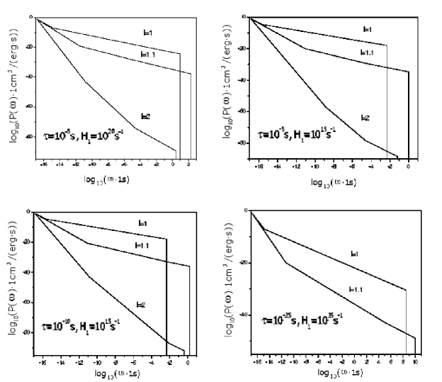
Figure 3.1: GWs spectrum for an expanding universe with a “MBHs+rad” era for certain values of $l$, $\tau$ and $H_{1}$. The spectrum predicted for the three-stage model of the previous section is plotted for comparison, $l=1$. Parameters $\tau$ and $H_{1}$ are chosen assuming each spectrum has the maximum value allowed by the CMB anisotropy data at the frequency $\omega=2\pi H_{0}=2.24\times 10^{-18}s^{-1}$. In the bottom-right panel the power spectrum with $l=2$ is rule out as it yields a CMB anisotropy larger than observed.

3.2.4 Restrictions on the “MBHs+rad” era from the cosmic microwave background

It is obvious that $\rho_{g}$ cannot be arbitrarily large, in fact the GWs are seen as linear perturbations of the metric. The linear approximation holds only for $\rho_{g}(\eta)\ll\rho(\eta)$, $\rho(\eta)$ being the total energy density of the Universe. Several observational data place constraints on $\rho_{g}$. The regularity of the pulses of stable millisecond pulsars sets a constraint at frequencies of order $10^{-8}Hz$ [40]. Likewise, there is a certain maximum value for $\rho_{g}$ compatible with the primordial nucleosynthesis scenario. But the most severe constraints come from the high isotropy degree of the CMB. We will focus on the latter constraint. The observed thermal fluctuations are usually analyzed by decomposing them into spherical harmonics

$$\frac{\delta T}{T}=\sum_{\ell,m}a_{\ell m}Y_{\ell m}(\theta,\phi),$$ (3.41)

where $a_{\ell m}$ are expansion coefficients and $\theta$ and $\phi$ are spherical polar angles on the sky. Defining the power spectrum by $C_{\ell}=\langle|a_{\ell m}|^{2}\rangle$, it is conventional to plot $\ell(\ell+1)C_{\ell}$ versus $\ell$. Figure 3.2 shows the first published results of the WMAP experiment regarding the CMB temperature anisotropies as well as the $\Lambda$CDM model (solid line) that fits the data rather well.

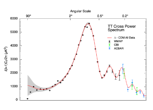
Figure 3.2: The CMB power spectrum from the WMAP satellite [41]. The error bars on this plot are 1-$\sigma$ and the solid line represents the best-fit cosmological model [39].

Metric perturbations with frequencies between $10^{-16}$ and $10^{-18}$ $Hz$ at the last scattering surface can produce thermal fluctuations in the CMB due to the Sachs-Wolfe effect [42]. These fluctuations cannot exceed the observed value of $\delta T/T\sim 5\times 10^{-6}$ [43].

A detailed analysis of the CMB bound yields [1, 44]

$$\Omega_{g}h_{100}^{2}<7\times 10^{-11}\left(\frac{H_{0}}{f}\right)^{2}{\qquad({H}_{0}<f<30\times H}_{0}{)}$$ (3.42)

where $\Omega_{g}=fP(f)/\rho_{0},$ $\rho_{0}=3cm_{Pl}^{2}H_{0}^{2}/(8\pi\hbar)$ and $H_{0}=h_{100}\times 100km/(s\times Mpc)$ with $h_{100}=0.7$. The CMB bound for the spectrum (3.34) evaluated at $2\pi H_{0}\,$Hertz reads

$$1>\left(2\pi\right)^{-4l}l^{2-4l}(2l^{2}-3l+1)^{2}\left(\frac{a_{1}}{a_{0}}\right)^{4l+4}\left(\frac{a_{0}}{a_{3}}\right)^{2}\left(\frac{H_{1}}{3.72\times 10^{19}s^{-1}}\right)^{3}\left(\frac{H_{1}}{H_{0}}\right)^{4l-1},$$ (3.43)

and consequently

$$f(l,H_{1},\tau)=-107.69+l\left(28.10+2\log_{10}\left(\frac{H_{1}}{1s^{-1}}\right)\right)-(2l-2)\log_{10}\left(1+\frac{l+1}{l}H_{1}\tau\right)$$ (3.44)

$$+(-4l+2)\log_{10}l+2\log_{10}(2l^{2}-3l+1)<0.$$

We next consider different values for $l$ and $\tau$.

(i) When $l=1.1$, the relation (3.44) reads

$$f(1.1,H_{1},\tau)=-76.71+2.20\log_{10}\left(\frac{H_{1}}{1s^{-1}}\right)-0.2\log_{10}\left(1+\frac{l+1}{l}H_{1}\tau\right)<0,$$ (3.45)

see Fig. 3.3. From it we observe that:

1. For $\tau<\tau_{c}^{l=1.1}=1.22\times 10^{-35}s$, the condition (3.45) is satisfied if $H_{1}<8.13\times 10^{34}s^{-1}$ and conflicts with (3.38), which in the most favorable case is $H_{1}=8.13\times 10^{34}s^{-1}$ for $\tau=\tau_{c}^{l=1.1}$. For $l=1.1$, there is no compatibility with the observed CMB anisotropy when $\tau<\tau_{c}^{l=1.1}$. Thus, this range of $\tau$ is ruled out.

2. For $\tau>\tau_{c}^{l=1.1}$, one obtains $H_{1}<H_{c}^{l=1.1}(\tau)$ from the condition (3.45). $H_{c}^{l=1.1}(\tau)$ is always larger than $\tau^{-1}$ in the range considered, e.g. $H_{c}^{l=1.1}(\tau=10^{-30}s)=2.40\times 10^{35}s^{-1}$. Taking into account (3.38) one obtains that the condition (3.45) is satisfied for $\tau^{-1}<H_{1}<H_{c}^{l=1.1}(\tau)$.

(ii) When $l=2$ (the extreme case in which the expansion is entirely dominated by the MBHs) we have

$$f(2,H_{1},\tau)=-51.89+4\log_{10}\left(\frac{H_{1}}{1s^{-1}}\right)-2\log_{10}\left(1+\frac{l+1}{l}H_{1}\tau\right)<0,$$ (3.46)

see figure 3.3. Inspection of (3.46) and Fig. 3.3 reveals that:

1. For $\tau<\tau_{c}^{l=2}=6.75\times 10^{-14}s$, one obtains $H_{1}<10^{13}s^{-1}$ which is totally incompatible with condition (3.38), $H_{1}>1.48\times 10^{13}s^{-1}$ for $\tau=\tau_{c}^{l=2}$ in the most favorable case. Thus, the region $\tau<\tau_{c}^{l=2}$ is ruled out as predicts an excess of anisotropy in the CMB.

2. For $\tau>\tau_{c}^{l=2}$, one obtains $H_{1}<H_{c}^{l=2}(\tau)$ from the condition (3.46). $H_{c}^{l=2}(\tau)$ is always larger than $1.48\times 10^{13}s^{-1}$ for $\tau$ in the range considered, e.g. $H_{c}^{l=2}(\tau=10^{-10}s)=1.35\times 10^{16}s^{-1}$. Conditions (3.38) and (3.46) are both satisfied in this range for $\tau^{-1}<H_{1}<H_{c}^{l=2}(\tau)$.

We may conclude by saying that the condition (3.44) leads to different allowed ranges for $H_{1}$ and $\tau$ for each $l$ considered, although their interpretation is rather similar. For $\tau<$ $\tau_{c}^{l}$ the condition of minimum duration of the  “MBHs+rad” era (3.38) and the upper bound given by the CMB anisotropy are incompatible. However, for $\tau>$ $\tau_{c}^{l}$ these two conditions are compatible for $\tau^{-1}<H_{1}<H_{c}^{l}(\tau)$.

Figure 3.3: The left panel depicts $f(1.1,H_{1},\tau)vs.\log_{10}H_{1}$ for a) $\tau=10^{-40}s$, b) $\tau=\tau_{c}^{l=1.1}=1.23\times 10^{-35}s$, and c) $\tau=10^{-30}s$. The right panel depicts $f(2,H_{1},\tau)$ for a) $\tau=10^{-20}s$, b) $\tau=\tau_{c1}^{l=2}=6.75\times 10^{-14}s$, and c) $\tau=10^{-10}s$. Conditions (3.44) and (3.38) are satisfied for certain ranges of $\tau$ and $H_{1}$ in each case.

3.3 Conclusions

We have calculated the power spectrum of GWs in a universe that begins with an inflationary phase, followed by a phase dominated by a mixture of MBHs and radiation, then a radiation dominated phase (after the MBHs evaporated), and finally a dust dominated phase. The spectrum depends just on three free parameters, namely $H_{1}$ the Hubble factor at the transition inflation- “MBHs+rad” era, $\tau$, the cosmological time span of the “MBHs+rad” era, and the power $l$, being $a(\eta)\propto\eta^{l}$ the scale factor of the “MBHs+rad” era with $1<l\leq 2$.

The upper bound on the spectrum of GWs obtained from the CMB anisotropy places severe constraints on $H_{1}$ and $\tau$. For each value of $l$ considered, there is a minimum value of $\tau$, $\tau_{c}^{l}$, compatible with the CMB anisotropy. There is a range of $\tau$, $\tau>\tau_{c}^{l}$, for which $\tau^{-1}<H_{1}<H_{c}^{l}(\tau)$ satisfies the CMB upper bound.

The four-stage scenario predicts a much lower power spectrum of GWs than the conventional three-stage scenario. If LISA fails to detect the GWs spectrum at the level predicted by the three-stage scenario, a possible explanation might be that the “MBHs+rad” era took place. Likewise, once the spectrum is successfully measured we will be able to learn from it the proportion of MBHs and radiation in the mixture phase as well as the time span of this era.

Chapter 4 Gravitational waves and present accelerated expansion

In this chapter we show how the power spectrum as well as the dimensionless density parameter of the GWs created from the initial vacuum state may help present (and future) observers ascertain whether the expansion phase they are living in is accelerated or not and if accelerated, which law follows the scale factor [45]. The latter would facilitate enormously to discriminate the nature of dark energy between a large variety of proposed models (cosmological constant, quintessence fields, interacting quintessence, tachyon fields, Chaplygin gas, etc) [46]. To this end we calculate the power spectrum and energy density of the GWs when the transitions to the dark energy era and second dust era are considered. Obviously, the latter power spectrum lies at the future and depending on the model under consideration it may take very long for the Universe to enter the second dust era.

4.1 Accelerated expansion and decaying dark energy

Nowadays the observational data regarding the apparent luminosity of supernovae type Ia, together with the discovery of CMB angular temperature fluctuations on degree scales and measurements of the power spectrum of galaxy clustering, strongly suggests that the Universe is nearly flat and that its expansion is accelerating at present [39, 47]. In actual fact the debate now focuses on when the acceleration did really commence, if it is just a transient phenomenon or it is to last forever, and above all the nature of the dark energy.

In Einstein gravity the accelerated expansion is commonly associated to a sufficiently high negative pressure which might be provided by a cosmological constant $\Lambda$ (vacuum energy), whose equation of state is $p_{\Lambda}=-\rho_{\Lambda}$, with $\rho_{\Lambda}=\Lambda/(8\pi)=\text{constant}$. The observational data seems to indicate that the cosmological constant contributes about the $70\%$ of the energy of the Universe, meanwhile the remaining $30\%$ comes from non-relativistic matter (i.e., dust). Thus, the question arises: “Why are the vacuum and matter energy densities of precisely the same order today?”, which is known in the literature as the coincidence problem [48].

A possible answer to this question considers that the acceleration of the Universe is associated to a sort of dynamical energy, the so–called dark energy, that violates the strong energy condition and clusters only at the largest accessible scales [46]. In such a case the present state of the Universe would be dominated by dark energy and since it redshifts more slowly with expansion than dust, the contribution of the latter is bound to become negligible at late times.

In an attempt to evade the particle horizon problem posed by an everlasting accelerated expansion to string/M type theories [49], some models propose dark energy potentials such that the current accelerated phase would be just transitory and sooner or later the expansion would revert to the Einstein–De Sitter law $a(t)\propto t^{2/3}$, thereby slowing down (second dust era) [50]. The possibility that dark energy could be unstable is in fact suggested by the remarkable qualitative analogy between the presence of dark energy today and the properties of a different type of dark energy - the inflaton field - postulated in the inflationary scenario of the early Universe -see e.g., [51]. This analogy has two main points. On one hand, it makes natural that a form of matter with negative pressure could have dominated the Universe in a distant past, since a similar form of matter dominates the Universe today. On the other hand, as the dark energy in the early Universe was unstable and decayed aeons ago, one might be tempted to ask whether the nature of dark energy observed today would be any different.

For our purposes, we shall assume a simplified model of decaying dark energy in which the usual dust dominated stage is followed by an accelerated era where the adiabatic index $\gamma$ of the fluid that dominates that era is a constant that lies in the range $[0,2/3)$. Posteriorly, the dark energy decays in a time span much lower than the duration of the accelerated era and the Universe resumes the decelerated expansion dominated by the cold dark matter. Models with dark energy whose evolution mimics that of dust can be also taken in consideration in our description as they are formally equivalent to the model of above.

4.2 Bogoliubov coefficients in the decaying dark energy scenario

In this section we evaluate the coefficients of Bogoliubov in the simplified model previously suggested, a spatially flat FRW scenario initially De Sitter, then dominated by radiation, followed by a dust dominated era, an accelerated expansion era dominated by dark energy, and finally a second dust era.

The scale factor in terms of the conformal time reads

$$a(\eta)=\left\{\begin{array}[]{lcr}-\frac{1}{H_{1}\eta}&(-\infty<\eta<\eta_{1}<0),&\text{De Sitter era}\\ \frac{1}{H_{1}\eta_{1}^{2}}(\eta-2\eta_{1})&(\eta_{1}<\eta<\eta_{2}),&\text{radiation era}\\ \frac{1}{4H_{1}\eta_{1}^{2}}\frac{(\eta+\eta_{2}-4\eta_{1})^{2}}{\eta_{2}-2\eta_{1}}&(\eta_{2}<\eta<\eta_{3}),&\text{first dust era}\\ \left(\frac{l}{2}\right)^{-l}\frac{(\eta_{3}+\eta_{2}-4\eta_{1})^{2-l}}{4H_{1}\eta_{1}^{2}(\eta_{2}-2\eta_{1})}\left(\eta_{l}\right)^{l}&(\eta_{3}<\eta<\eta_{4}),&\text{dark energy era}\\ \frac{a_{4}}{4}\left(a_{4}H_{4}\right)^{2}\left(\eta-\eta_{4}+\frac{2}{a_{4}H_{4}}\right)^{2}&(\eta_{4}<\eta),&\text{second dust era}\end{array}\right.$$ (4.1)

where $l\leq-1$, $\eta_{l}=\eta+\frac{l}{2}\left[\left(-2/l+1\right)\eta_{3}+\eta_{2}-4\eta_{1}\right]$, the subindexes $1,2,3,4$ correspond to sudden transitions from inflation to radiation era, from radiation to first dust era, from first dust era to dark energy era and from the latter to the second dust era, respectively; $H_{i}$ is the Hubble factor at the instant $\eta=\eta_{i}$. The present time $\eta_{0}$ lies in the range $\left[\eta_{3},\eta_{4}\right]$, it is to say in the dark energy dominated era.

GWs which are inside the Hubble radius have a wave number $k$ lower than $a(\eta)H(\eta)$. Figure 4.1 sketches the evolution of $a(\eta)H(\eta)$ in this scenario. During the inflationary and dark energy eras $a(\eta)H(\eta)$ increases with $\eta$, and decreases in the other eras. As a consequence, $a_{4}H_{4}$ results higher than $a_{3}H_{3}$. Choosing $l$, $\eta_{3}$ and $\eta_{4}$ in such a way that

$$\left(\frac{a_{4}}{a_{3}}\right)^{-1/l}\left(\frac{a_{2}}{a_{3}}\right)^{1/2}>1,$$ (4.2)

we have that $a_{4}H_{4}$ is also higher than $a_{2}H_{2}$. We assume that $a_{4}H_{4}$ is lower than $a_{1}H_{1}$ throughout.

Figure 4.1: Evolution of $a(\eta)H(\eta)$ in a universe with scale factor given by Eq. (4.1) under the assumption $a_{4}H_{4}>a_{2}H_{2}$. The quantity $\eta_{f0}$ is defined as the instant in the dark energy era in which $a(\eta_{f0})H(\eta_{f0})=a_{2}H_{2}$, $\eta_{f1}$ as the instant of the second dust era such that $a(\eta_{f1})H(\eta_{f1})=a_{2}H_{2},$ and $\eta_{f2}$ as the instant of the second dust era in which $a(\eta_{f0})H(\eta_{f0})=a_{3}H_{3}$.

The scale factor (4.1) formally coincides with these of the standard three-stage model given by (3.1) until the instant $\eta_{3}$. Thus, the Bogoliubov coefficients $\alpha_{1}$ and $\beta_{1}$ are equal to those of equation (3.5) in the range $k<2\pi a_{1}H_{1}$ and they are $1$ and $0$ for $k>a_{1}H_{1}$, respectively. Analogously, $\alpha_{2}$ and $\beta_{2}$ coincides with those of (3.8) for $k<2\pi a_{2}H_{2}$ and are $1$ and $0$ for $k>a_{2}H_{2}$.

In the dark energy era the solution to Lifshitz’s equation (2.10) reads

$$\mu_{l}=(\sqrt{\pi}/2)e^{i\psi_{l}}k^{-1/2}x_{l}^{1/2}H_{l-1/2}^{(2)}(x_{l}),$$ (4.3)

where $x_{l}=k\eta_{l}$. The Bogoliubov transformation

$$\mu_{D}(\eta)=\alpha_{3}^{l}\mu_{l}(\eta)+\beta_{3}^{l}\mu_{l}^{\ast}(\eta)$$ (4.4)

relates the dust and dark energy modes.

Using the well-known relation for Hankel functions [36]

$$H_{l-1/2}^{(2)}(x)\simeq e^{-ix}\sqrt{\frac{2}{\pi x}}\frac{(-2l)!}{(-l)!}(-2)^{l}x^{l}(1+ix),$$ (4.5)

valid when $x\ll 1$ and $l<-1$, it follows that

$$\alpha_{3} = \left(6(-1)^{-l}l^{l}\frac{(-2l)!}{(-l)!}\right)\eta_{m3}^{l-2}k^{l-2}+\mathcal{O}(k^{l-1}),$$

$$\beta_{3} = -\left(6(-1)^{-l}l^{l}\frac{(-2l)!}{(-l)!}\right)\eta_{m3}^{l-2}k^{l-2}+\mathcal{O}(k^{l-1}),$$

for $k<2\pi a(\eta_{3})H_{3}$ and $\alpha_{3}=1$, $\beta_{3}=0$ for $k>2\pi a(\eta_{3})H_{3}$, where $H_{3}$ is the Hubble function evaluated at $\eta_{3}$ and $\eta_{m3}=\eta_{3}+\eta_{2}-4\eta_{1}$. The transition between the first dust era to the dark energy era has a time span of the order $H_{3}^{-1}$. This is much shorter than the period of the waves we are considering and therefore it may be assumed instantaneous when calculating the coefficients. As a consequence, the time span from this transition till today, $\tau=t_{0}-t_{3}$, must be larger than $H_{3}^{-1}$, otherwise the transition first dust era-dark energy era would be too close to the present time for our formalism to apply. This condition places a lower bound on the value of the redshift $\frac{a_{0}}{a_{3}}$. When $l=-1$ the condition is $\frac{a_{0}}{a_{3}}>2.72$, $\frac{a_{0}}{a_{3}}>2.25$ when $l=-2$, $\frac{a_{0}}{a_{3}}>2.15$ when $l=-3$, and $\frac{a_{0}}{a_{3}}>2$ when $l\rightarrow-\infty$. This bound is compatible with the accepted values for $\frac{a_{0}}{a_{3}}\in[1.5,11]$ (see e.g., [52]). Henceforward we will consider $\frac{a_{0}}{a_{3}}$ larger than $2.72$ and no larger than $11$.

The solution to Lifshitz’s equation in the second dust era (i.e., the one following the dark energy era) is

$$\mu_{SD}=(\sqrt{\pi}/2)e^{i\psi_{SD}}k^{-1/2}x_{SD}^{1/2}H_{3/2}^{(2)}(x_{SD}),$$ (4.6)

where $x_{SD}=k\left(\eta-\eta_{4}+\frac{2}{a_{4}H_{4}}\right)$.

The Bogoliubov coefficients relating the modes of the dark energy era with the modes of the second dust era are

$$\mu_{l}(\eta)=\alpha_{4}^{l}\mu_{SD}(\eta)+\beta_{4}^{l}\mu_{SD}^{\ast}(\eta).$$ (4.7)

Likewise, the continuity of $\mu$ at $\eta_{4}$ implies

$$\alpha_{4}^{l} = \left(-1\right)^{l}\frac{3}{8}2^{l}\frac{(-2l)!}{(-l)!}x_{l4}^{l-2}\left[l^{2}+il(l-2)x_{l4}+\mathcal{O}(x_{l4}^{2})\right],$$

$$\beta_{4}^{l} = \left(-1\right)^{l}\frac{3}{8}2^{l}\frac{(-2l)!}{(-l)!}x_{l4}^{l-2}\left[l^{2}+il(l+2)x_{l4}+\mathcal{O}(x_{l4}^{2})\right],$$

for $k<2\pi a_{4}H_{4}$, and $\alpha_{4}^{l}=1$, $\beta_{4}^{l}=0$ for $k>2\pi a_{4}H_{4}$, where $H_{4}$ is the Hubble function evaluated at the transition time $\eta_{4}$.

4.3 Power spectrums

In this section we evaluate the total coefficients and calculate the current power spectrum as well as the power spectrum in the second dust era. We find that the current power spectrum coincides with those of the three-stage model of section 3.1 but it evolves differently. We also find two possible shapes for the power spectrum in the second dust era, whether condition (4.2) is fulfilled or not.

4.3.1 Current power spectrum

To evaluate the present power spectrum one must bear in mind that $a_{0}H_{0}>a_{3}H_{3}$ which implies the wave lengths of the perturbations created at the transition dust era-dark energy era are larger than the present Hubble radius $H_{0}^{-1}$ [53]. One must also consider the possibility that $a_{0}H_{0}>a_{2}H_{2}$, it is to say

$$\left(\frac{a_{0}}{a_{3}}\right)^{-1/l}\left(\frac{a_{2}}{a_{3}}\right)^{1/2}>1.$$ (4.8)

For $l=-1$ and assuming $\frac{a_{0}}{a_{2}}\sim 10^{4}$ [38] this condition implies $\frac{a_{0}}{a_{3}}>21.5$, $\frac{a_{0}}{a_{3}}>100$ when $l=-2,$ and $\frac{a_{0}}{a_{3}}>251.2$ when $l=-3$. The values for $\frac{a_{0}}{a_{3}}$ considered by us are larger than $2.72$ and no lower than $11$, consequently we can safely assume $a_{0}H_{0}<a_{2}H_{2}$.

For $k>2\pi a_{1}H_{1}$, we find that $\alpha_{Tr2}=1$, $\beta_{Tr2}=0$; in the range $2\pi a_{1}H_{1}>k>2\pi a_{2}H_{2}$, the coefficients are $\alpha_{Tr2}=\alpha_{1}$ and $\beta_{Tr2}=\beta_{1}$, and finally for $k<2\pi a(\eta_{2})H_{2}$ we obtain [27, 24]

$$\beta_{Tr2}\simeq-\frac{1}{8k^{3}\eta_{1}^{2}\eta_{R2}}.$$ (4.9)

Thus, the number of GWs at the present time $\eta_{0}$ created from the initial vacuum state is $\left\langle N_{\omega}\right\rangle=\left|\beta_{Tr2}\right|^{2}\sim\omega^{-6}(\eta_{0})$ for $\omega(\eta_{0})<2\pi(a_{2}/a_{0})H_{2}$, $\omega^{-4}(\eta_{0})$ for $2\pi(a_{1}/a_{0})H_{1}>\omega(\eta_{0})>2\pi(a_{2}/a_{0})H_{2}$, and zero for $\omega(\eta_{0})>2\pi(a_{1}/a_{0})H_{1}$, where we have used the present value of the frequency, $\omega(\eta_{0})=k/a_{0}$.

In summary, the current power spectrum of GWs in this scenario is

$$P(\omega)\simeq\left\{\begin{array}[]{l}0\text{\qquad}\left(\omega(\eta_{0})>2\pi(a_{1}/a_{0})H_{1}\right),\\ \\ \frac{1}{4\pi^{2}}\left(\frac{a_{1}}{a_{0}}\right)^{4}H_{1}^{4}\omega^{-1}\text{\qquad}\left(2\pi(a_{2}/a_{0})H_{2}<\omega(\eta_{0})<2\pi(a_{1}/a_{0})H_{1}\right),\\ \\ \frac{1}{16\pi^{2}}\left(\frac{a_{0}}{a_{2}}\right)^{2}\left(\frac{a_{1}}{a_{0}}\right)^{8}H_{1}^{6}\omega^{-3}\text{\qquad}\left(2\pi H_{0}<\omega(\eta_{0})<2\pi(a_{2}/a_{0})H_{2}\right).\end{array}\right.$$ (4.10)

While this power spectrum is not at variance with the power spectrum of the conventional three-stage scenario evaluated at section 3.1, it evolves differently. The power spectrum in the dark energy scenario at $\eta=\eta_{3}$ formally coincides with Eq. (4.10) but with $a_{3}$ substituted by $a_{0}$ throughout, and from then up to now waves with $2\pi a_{3}H_{3}<k<$ $2\pi a_{0}H_{0}$ cease to contribute to the spectrum as soon as their wave length exceeds the Hubble radius. By contrast, in the three-stage scenario waves are continuously being added to the spectrum. As we shall see in section 4.4, this implies that the evolution of the energy density of the gravitational waves in the three-stage scenario differs from the scenario in which the Universe expansion is dominated by dark energy.

4.3.2 Power spectrum in the second dust era

Here we evaluate the power spectrum at some future time $\eta$ larger than $\eta_{f2}$ for which the waves created at the transition dust era-dark energy era ($\eta=\eta_{3}$) are considered in the spectrum by the first time (see Figure 4.1). Let $\alpha_{Tr4}$ and $\beta_{Tr4}$ be the Bogoliubov coefficients relating the modes of the inflationary era to the modes of the second dust era. Because of condition (4.2) we must consider two possibilities with two different power spectrums.

$(i)$ If condition (4.2) is not fulfilled, then $a_{1}H_{1}>a_{2}H_{2}>a_{4}H_{4}>a_{3}H_{3}$ and the power spectrum can be obtained from the following total coefficients. In the range $k>2\pi a_{1}H_{1}$ the total coefficients are $\alpha_{Tr4}=1$ and $\beta_{Tr4}=0$. For $2\pi a_{1}H_{1}>k>2\pi a_{2}H_{2}$, the coefficients are $\alpha_{Tr4}=\alpha_{1}$ and $\beta_{Tr4}=\beta_{1}$, where $\alpha_{1}$ and $\beta_{1}$ are defined in Eq. (3.5). For $2\pi a_{2}H_{2}>k>2\pi a_{4}H_{4}$, $\alpha_{Tr4}=\alpha_{Tr2}$ and $\beta_{Tr4}=\beta_{Tr2}$ where $\beta_{Tr2}$ is defined in Eq. (4.9) and the dominant term of $\alpha_{Tr2}$ coincides with $\beta_{Tr2}$.

When $2\pi a_{4}H_{4}>k>2\pi a_{3}H_{3}$, except for $\alpha_{3}$ and $\beta_{3}$, all the coefficients obtained in the previous section must be considered when evaluating $\alpha_{Tr4}$ and $\beta_{Tr4}$, therefore

$$\alpha_{Tr4}^{l} = \alpha_{4}^{l}\alpha_{Tr2}+\beta_{4}^{l\ast}\beta_{Tr2}\simeq\left[\frac{3}{32}\left(-1\right)^{-l-1}l^{2}2^{l}\frac{(-2l)!}{(-l)!}\right]\frac{2}{\eta_{1}^{2}\eta_{R2}\eta_{l4}^{-l+2}}k^{l-5},\qquad$$ (4.11)

$$\beta_{Tr4}^{l} = \beta_{4}^{l}\alpha_{Tr2}+\alpha_{4}^{l\ast}\beta_{Tr2}\simeq\left[\frac{3}{32}\left(-1\right)^{-l-1}l^{2}2^{l}\frac{(-2l)!}{(-l)!}\right]\frac{2}{\eta_{1}^{2}\eta_{R2}\eta_{l4}^{-l+2}}k^{l-5}.$$ (4.12)

Finally, for $2\pi a_{3}H_{3}>k>2\pi H(\eta)$, we get

$$\beta_{Tr4}^{l}\simeq-\left[\frac{9}{16}l^{l+2}2^{l}\left(\frac{(-2l)!}{(-l)!}\right)^{2}\right]\frac{2l}{\eta_{1}^{2}\eta_{R2}\eta_{m3}^{-l}\eta_{l4}^{-l+2}}k^{2l-5}.$$ (4.13)

Accordingly, the power spectrum reads

$$P(\omega)\simeq\left\{\begin{array}[]{l}0\text{\qquad}\left(\omega(\eta)>2\pi(a_{1}/a(\eta))H_{1}\right),\\ \\ \frac{1}{4\pi^{2}}\left(\frac{a_{1}}{a(\eta)}\right)^{4}H_{1}^{4}\omega^{-1}\text{\qquad}\left(2\pi(a_{2}/a(\eta))H_{2}<\omega(\eta)<2\pi(a_{1}/a(\eta))H_{1}\right),\\ \\ \frac{1}{16\pi^{2}}\left(\frac{a_{0}}{a_{2}}\right)^{2}\left(\frac{a_{1}}{a_{0}}\right)^{8}\left(\frac{a_{0}}{a(\eta)}\right)^{6}H_{1}^{6}\omega^{-3}\text{\qquad}\left(2\pi(a_{4}/a(\eta))H_{4}<\omega(\eta)<2\pi(a_{2}/a(\eta))H_{2}\right)\\ \\ \frac{9}{\pi^{2}}l^{2l}2^{2l-8}\left(\frac{(-2l)!}{(-l)!}\right)^{2}\left(\frac{a_{1}}{a_{0}}\right)^{16-4l}\left(\frac{a_{2}}{a_{0}}\right)^{l-4}\left(\frac{a_{3}}{a_{0}}\right)^{l-4+4/l}\left(\frac{a_{4}}{a_{0}}\right)^{-8+2l-4/l}\\ \text{\qquad}\times\left(\frac{a(\eta)}{a_{4}}\right)^{2l-10}H_{1}^{10-2l}\omega^{2l-7}\text{\qquad}\left(2\pi(a_{3}/a(\eta))H_{3}<\omega(\eta)<2\pi(a_{4}/a(\eta))H_{4}\right),\\ \\ \frac{27}{\pi^{2}}l^{4l}2^{4l-6}\left(\frac{(-2l)!}{(-l)!}\right)^{4}\left(\frac{a_{1}}{a_{0}}\right)^{16-8l}\left(\frac{a_{2}}{a_{0}}\right)^{2l-4}\left(\frac{a_{3}}{a_{0}}\right)^{2l-4+4/l}\left(\frac{a_{4}}{a_{0}}\right)^{4l-8-4/l}\\ \text{\qquad}\times\left(\frac{a(\eta)}{a_{4}}\right)^{4l-10}H_{1}^{10-4l}\omega^{4l-7}\text{\qquad}\left(2\pi H(\eta)<\omega(\eta)<2\pi(a_{3}/a(\eta))H_{3}\right).\end{array}\right.$$ (4.14)

$(ii)$ If condition (4.2) is fulfilled, then $a_{1}H_{1}>a_{4}H_{4}>a_{2}H_{2}>a_{3}H_{3}$. As in the previous case, in the range $k>2\pi a_{1}H_{1}$ the total coefficients are $\alpha_{Tr4}=1$ and $\beta_{Tr4}=0$. For $2\pi a_{1}H_{1}>k>2\pi a_{4}H_{4}$, the coefficients are $\alpha_{Tr4}=\alpha_{1}$ and $\beta_{Tr4}=\beta_{1}$. In the range $2\pi a_{4}H_{4}>k>2\pi a_{2}H_{2}$, we obtain

$$\alpha_{Tr4}^{l} = \alpha_{4}^{l}\alpha_{1}+\beta_{4}^{l\ast}\beta_{1}\simeq i\frac{3}{8}\left(-1\right)^{-l}l^{2}2^{l}\frac{(-2l)!}{(-l)!}\frac{1}{\eta_{1}^{2}\eta_{l4}^{-l+1}}k^{l-3},\qquad$$

$$\beta_{Tr4}^{l} = \beta_{4}^{l}\alpha_{1}+\alpha_{4}^{l\ast}\beta_{1}\simeq i\frac{3}{8}\left(-1\right)^{-l}l^{2}2^{l}\frac{(-2l)!}{(-l)!}\frac{1}{\eta_{1}^{2}\eta_{l4}^{-l+1}}k^{l-3}.$$

Again, for $2\pi a_{2}H_{2}>k>2\pi a_{3}H_{3}$, the total coefficients are given by Eq. (4.11) while for $2\pi a_{3}H_{3}>k>2\pi H(\eta)$ they obey Eq. (4.13). The power spectrum in this case is

$$P(\omega)\simeq\left\{\begin{array}[]{l}0\text{\qquad}\left(\omega(\eta)>2\pi(a_{1}/a(\eta))H_{1}\right),\\ \\ \frac{1}{4\pi^{2}}\left(\frac{a_{1}}{a(\eta)}\right)^{4}H_{1}^{4}\omega^{-1}\text{\qquad}\left(2\pi(a_{4}/a(\eta))H_{4}<\omega(\eta)<2\pi(a_{1}/a(\eta))H_{1}\right),\\ \\ \frac{9}{\pi^{2}}l^{2l+2}2^{2l-6}\left(\frac{(-2l)!}{(-l)!}\right)^{2}\left(\frac{a_{1}}{a_{0}}\right)^{8-4l}\left(\frac{a_{2}}{a_{0}}\right)^{l-1}\left(\frac{a_{3}}{a_{0}}\right)^{l-3+2/l}\left(\frac{a_{4}}{a_{0}}\right)^{2l-4-4/l}\\ \text{\qquad}\times\left(\frac{a(\eta)}{a_{4}}\right)^{2l-6}H_{1}^{6-2l}\omega^{2l-3}\text{\qquad}\left(2\pi(a_{2}/a(\eta))H_{2}<\omega(\eta)<2\pi(a_{4}/a(\eta))H_{4}\right),\\ \\ \frac{9}{\pi^{2}}l^{2l}2^{2l-8}\left(\frac{(-2l)!}{(-l)!}\right)^{2}\left(\frac{a_{1}}{a_{0}}\right)^{16-4l}\left(\frac{a_{2}}{a_{0}}\right)^{l-4}\left(\frac{a_{3}}{a_{0}}\right)^{l-4+4/l}\left(\frac{a_{4}}{a_{0}}\right)^{2l-8-4/l}\\ \text{\qquad}\times\left(\frac{a(\eta)}{a_{4}}\right)^{2l-10}H_{1}^{10-2l}\omega^{2l-7}\text{\qquad}\left(2\pi(a_{3}/a(\eta))H_{3}<\omega(\eta)<2\pi(a_{2}/a(\eta))H_{2}\right),\\ \\ \frac{27}{\pi^{2}}l^{4l}2^{4l-6}\left(\frac{(-2l)!}{(-l)!}\right)^{4}\left(\frac{a_{1}}{a_{0}}\right)^{16-8l}\left(\frac{a_{2}}{a_{0}}\right)^{2l-4}\left(\frac{a_{3}}{a_{0}}\right)^{2l-4+4/l}\left(\frac{a_{4}}{a_{0}}\right)^{4l-8-4/l}\\ \text{\qquad}\times\left(\frac{a(\eta)}{a_{4}}\right)^{4l-10}H_{1}^{10-4l}\omega^{4l-7}\text{\qquad}\left(2\pi H(\eta)<\omega(\eta)<2\pi(a_{3}/a(\eta))H_{3}\right).\end{array}\right.$$ (4.15)

The power spectrum governed by Eq.(4.15) is plotted in Fig. 4.2 for different choices of the free parameters $l$, $\frac{a_{0}}{a_{3}}$, $\frac{a_{4}}{a_{0}}$ and $\frac{a(\eta)}{a_{0}}$ as well as the power spectrum assuming the three-stage model, i.e., non-accelerated phase and no second dust era.

The shape of the power spectrum given by (4.15) in the range $2\pi H(\eta)<\omega(\eta)<2\pi(a_{3}/a(\eta))H_{3}$ is the same in both cases as in this range all the coefficients are present in the evaluation of the total coefficients. It is interesting to see how markedly this spectrum differs from the one arising in the three-stage model (dot-dashed line) at low frequencies.

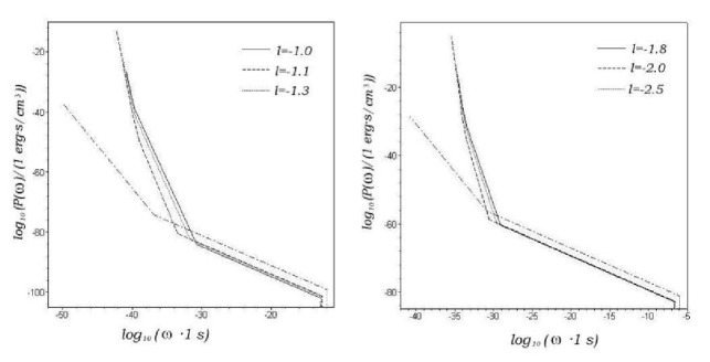
Figure 4.2: Power spectrum given by Eq. (4.15) for different values of $l$. The left panel depicts the power spectrum at the instant $\eta$ for which $\frac{a\left(\eta\right)}{a_{0}}=10^{22}$ (when $\Omega_{g}(\eta)$ is near unity), with $\frac{a_{0}}{a_{3}}=11$, and $\frac{a_{4}}{a_{0}}=10^{6}$ (to fulfill condition (4.2)). The right panel shows the power spectrum at the instant $\eta$ for which $\frac{a\left(\eta\right)}{a_{0}}=10^{16}$ (again when $\Omega_{g}(\eta)$ is near unity), with $\frac{a_{0}}{a_{3}}=11$, and $\frac{a_{4}}{a_{0}}=10^{6}$. For the sake of comparison the power spectrum of the three-stage scenario (De Sitter inflation, radiation, dust with $l=2$) is also shown in both panels (dot-dashed line). Notice the difference in slopes at the dust era.

Topological defects

Up to now we assumed that at the end of the dark energy era the Universe will evolve as if it became dominated by dust once again. Nevertheless if the expansion achieved in the accelerated phase were large enough, either cosmic strings, or domain walls, or a cosmological constant will take over instead. We will not consider, however, cosmic strings (whose equation of state is $p_{K}=-\frac{1}{3}\rho_{K}$) for, as pointed out by Maia [24], it seems problematic to define an adiabatic vacuum in an era dominated by these topological defects since the creation–annihilation operators, $A_{(k)}$, $A_{(k)}^{{\dagger}}$, fail to satisfy the commutation relations (i.e., condition (2.29)) in the range of frequencies where one should expect GWs amplification. In short, our approach, as it is, does not apply to this case.

As for domain walls (topological stable defects of second order with equation of state $p_{dw}=-\frac{2}{3}\rho_{dw}$ and energy density that varies as $a^{-1}(\eta)$ -see e.g., [51, 54]), once the dark energy evolved as pressureless matter at $\eta=\eta_{4}$ the scale factor may be approximated by

$$a(\eta>\eta_{4})=4a_{4}\left(a_{4}H_{4}\right)^{-2}\left(-\eta+\eta_{4}+\frac{2}{a_{4}H_{4}}\right)^{-2},$$ (4.16)

so long as $a^{-1}\gg a^{-3}$. That is to say, for $\eta>\eta_{4}$ the expansion of the Universe is again accelerated whereby $a(\eta)H(\eta)$ resumes growing. The GWs will be leaving the Hubble radius as soon as $H^{-1}$ becomes smaller than their wave length, and eventually none of them will contribute to the spectrum.

Finally, we consider the existence of a positive cosmological constant $\Lambda$. (Recall that $\rho_{\Lambda}=\Lambda/\left(8\pi\right)$ and $p_{\Lambda}=-\rho_{\Lambda}$). Once the dark energy dynamically mimicked dust the Universe will become dominated by a very tiny cosmological constant. The corresponding scale factor is

$$a(\eta>\eta_{4})=H_{4}^{-1}\left(-\eta+\eta_{4}+\frac{1}{a_{4}H_{4}}\right)^{-1}.$$ (4.17)

Once again, the expansion is accelerated and GWs will leave the Hubble radius and, in the long run, none of them will contribute to the spectrum.

4.4 Energy density of the gravitational waves

Now we are in position to evaluate the energy density of the GWs in terms of the conformal time by integrating the power spectrum $P(\omega)$ obtained in the previous section. As we shall see, the evolution of the energy density strongly depends on the free parameters of the model.

Its current value, evaluated from Eq. (4.10), can be approximated by [27]

$$\rho_{g}(\eta_{0})\simeq\frac{\hbar}{32\pi^{2}c^{3}}\left(\frac{a_{0}}{a_{2}}\right)^{2}\left(\frac{a_{1}}{a_{0}}\right)^{8}H_{1}^{6}(2\pi H_{0})^{-2}.$$ (4.18)

where, in this section, we return to conventional units.

To study the evolution of $\rho_{g}(\eta)$ from this point onward we first consider that $a_{4}H_{4}>a_{2}H_{2}$. In this case, $\rho_{g}(\eta)$ evolves as (4.18) with $H(\eta)$ and $a(\eta)$ substituted by $H_{0}$ and $a_{0}$, respectively, till some instant $\eta_{f0}$ in the range $\eta_{0}<\eta_{f0}<\eta_{4}$. When $\eta\geqslant\eta_{f0}$ the GWs with $\omega(\eta_{f0})<2\pi\left(a_{2}/a(\eta_{f0})\right)H_{2}$ must no longer be considered in evaluating $\rho_{g}$ as their wave length exceed the Hubble radius. Consequently

$$\rho_{g}(\eta_{f0}<\eta<\eta_{4})\simeq\frac{\hbar}{4\pi^{2}c^{3}}\left(\frac{a_{1}}{a(\eta)}\right)^{4}H_{1}^{4}\ln\left(\frac{a_{1}H_{1}}{a(\eta)H(\eta)}\right).$$ (4.19)

For $\eta=\eta_{4}$, the gravitational waves created at the transition dark energy era-second dust era begin contributing to $\rho_{g}$ thereby,

$$\rho_{g}(\eta_{4} < \eta<\eta_{f1})\simeq\rho_{g}(\eta_{4})\left(\frac{a_{4}}{a\left(\eta\right)}\right)^{4}+\frac{9\hbar}{\pi^{2}c^{3}}l^{2l+2}2^{2l-6}\left(\frac{(-2l)!}{(-l)!}\right)^{2}\left(\frac{a_{1}}{a_{0}}\right)^{8-4l}$$

$$\times\left(\frac{a_{2}}{a_{0}}\right)^{l-1}\left(\frac{a_{3}}{a_{0}}\right)^{l-3+2/l}\left(\frac{a_{4}}{a_{0}}\right)^{2l-4-4/l}\left(\frac{a(\eta)}{a_{4}}\right)^{2l-6}H_{1}^{6-2l}\frac{(2\pi H(\eta))^{2l-2}}{-2l+2},$$

where $\rho_{g}(\eta_{4})$ corresponds to Eq.(4.19) evaluated at $\eta=\eta_{4}$. For $\eta=\eta_{f1}>\eta_{4}$ where $\eta_{f1}$ is defined by the condition $a(\eta_{f1})H(\eta_{f1})=a_{2}H_{2}$ (see Figure 4.1), the gravitational waves which left the Hubble radius at $\eta_{f0}$ reenter it, therefore

$$\rho_{g}(\eta_{f1} < \eta<\eta_{f2})\simeq\rho_{g}(\eta_{f1})\left(\frac{a_{f1}}{a\left(\eta\right)}\right)^{4}+\frac{9\hbar}{\pi^{2}c^{3}}l^{2l}2^{2l-8}\left(\frac{(-2l)!}{(-l)!}\right)^{2}\left(\frac{a_{1}}{a_{0}}\right)^{16-4l}$$

$$\times\left(\frac{a_{2}}{a_{0}}\right)^{l-4}\left(\frac{a_{3}}{a_{0}}\right)^{l-4+4/l}\left(\frac{a_{4}}{a_{0}}\right)^{2l-8-4/l}\left(\frac{a(\eta)}{a_{4}}\right)^{2l-10}H_{1}^{10-2l}\frac{(2\pi H(\eta))^{2l-6}}{-2l+6},$$

where $\rho_{g}(\eta_{f1})$ corresponds to Eq.(4.4) evaluated at $\eta=\eta_{f1}$. For $\eta=\eta_{f2}$, with $\eta_{f2}$ defined by $a(\eta_{f2})H(\eta_{f2})=a_{3}H_{3}$ (see Figure 4.1), the gravitational waves created at the transition first dust era-dark energy era have wave lengths shorter than the Hubble radius for first time, and from that point on the density of gravitational waves can be approximated by

$$\rho_{g}(\eta > \eta_{f2})\simeq\rho_{g}(\eta_{f2})\left(\frac{a_{f2}}{a\left(\eta\right)}\right)^{4}+\frac{27\hbar}{\pi^{2}c^{3}}l^{4l}2^{4l-6}\left(\frac{(-2l)!}{(-l)!}\right)^{4}\left(\frac{a_{1}}{a_{0}}\right)^{16-8l}$$

$$\times\left(\frac{a_{2}}{a_{0}}\right)^{2l-4}\left(\frac{a_{3}}{a_{0}}\right)^{2l-4+4/l}\left(\frac{a_{4}}{a_{0}}\right)^{4l-8-4/l}\left(\frac{a(\eta)}{a_{4}}\right)^{4l-10}H_{1}^{10-4l}\frac{(2\pi H(\eta))^{4l-6}}{-4l+6},$$

where $\rho_{g}(\eta_{f2})$ corresponds to Eq.(4.4) evaluated at $\eta=\eta_{f2}$.

In the case that $a_{4}H_{4}>a_{2}H_{2}$, Eq. (4.18) dictates the evolution of $\rho_{g}$ between $\eta_{0}$ till $\eta_{4}$. Then, from $\eta_{4}$ till $\eta_{f2}$, $\rho_{g}$ obeys Eq. (4.4) (note that $\eta_{f1}$ cannot be defined in this case) and from $\eta_{f2}$ onwards $\rho_{g}$ obeys Eq. (4.4).

A natural restriction on $\rho_{g}(\eta)$ is that it must be lower than the total energy density of the flat FRW universe

$$\rho(\eta)=\frac{c}{\hbar}\frac{3m_{Pl}^{2}}{8\pi}H^{2}(\eta),$$ (4.23)

where $m_{Pl}=\sqrt{\hbar c/G}$ stands for the Planck mass.

It seems reasonable to consider $H_{1}\simeq 10^{38}s^{-1}$ as it corresponds to the grand unification energy scale of inflationary models [1, 51, 55]. The redshift $\frac{a_{0}}{a_{2}}$, relating the present value of the scale factor with the scale factor at the transition radiation era-first dust era, may be taken as $10^{4}$ [38], and the current value of the Hubble factor $H_{0}$ is estimated to be $2.24\times 10^{-18}s^{-1}$ [39, 56]. It then follows

$$\frac{a_{1}}{a_{0}} = 1.50\times 10^{-29}\left(\frac{a_{0}}{a_{3}}\right)^{-\frac{1}{4}+\frac{1}{2l}},\text{\qquad}H_{2}=2.24\times 10^{-12}\left(\frac{a_{0}}{a_{3}}\right)^{-\frac{1}{2}+\frac{1}{l}}s^{-1},$$

$$H_{3} = H_{0}\left(\frac{a_{0}}{a_{3}}\right)^{1+\frac{1}{l}}s^{-1},\text{\qquad}H_{4}=H_{0}\left(\frac{a_{4}}{a_{0}}\right)^{-1-\frac{1}{l}}s^{-1},$$

$$H_{f1} = 2.24\times 10^{-12}\left(\frac{a_{0}}{a_{3}}\right)^{-\frac{3}{2}+\frac{3}{l}}\left(\frac{a_{4}}{a_{0}}\right)^{-1+\frac{2}{l}}s^{-1},$$

$$H_{f2} = 2.24\times 10^{-18}\left(\frac{a_{0}}{a_{3}}\right)^{\frac{3}{l}}\left(\frac{a_{4}}{a_{0}}\right)^{-1+\frac{2}{l}}s^{-1},$$

where we have used the relation

$$H(\eta>\eta_{4})=\left(\frac{a_{4}}{a(\eta)}\right)^{3/2}H_{4},$$ (4.24)

valid in the second dust era (see Eq. (4.1)) with $a_{f1}H_{f1}=a_{2}H_{2}$ and $a_{f2}H_{f2}=a_{3}H_{3}$ to evaluate $H_{f1}$ (only defined if $a_{4}H_{4}>a_{2}H_{2}$) and $H_{f2}$, respectively. In our model, there are only three parameters, namely $l\leq-1$, $2.72<\frac{a_{0}}{a_{3}}<11$, and $\frac{a_{4}}{a_{0}}$.

We are now in position to evaluate the evolution of the dimensionless density parameter $\Omega_{g}(\eta)\equiv\rho_{g}(\eta)/\rho(\eta)$. Its current value is [27]

$$\Omega_{g0}\simeq\frac{1}{48\pi^{3}}\frac{G\hbar}{c^{5}}\left(\frac{a_{0}}{a_{2}}\right)^{2}\left(\frac{a_{1}}{a_{0}}\right)^{8}H_{1}^{6}H_{0}^{-4},$$ (4.25)

which in our description boils down to

$$\Omega_{g0}\simeq 2.00\times 10^{-13}\left(\frac{a_{0}}{a_{3}}\right)^{-2+\frac{4}{l}}.$$ (4.26)

$\Omega_{g0}$ is much lower than unity for any choice of $\frac{a_{0}}{a_{3}}$ and $l$ in the above intervals. At later times $\Omega_{g}$ evolves as

$$\Omega_{g}(\eta>\eta_{0})=\Omega_{g0}\left(\frac{a(\eta)}{a_{0}}\right)^{-2+\frac{4}{l}},$$ (4.27)

where we have used $H(\eta_{4}>\eta>\eta_{0})=\left(\frac{a(\eta)}{a_{0}}\right)^{-1-\frac{1}{l}}H_{0}$. It is obvious that $\Omega_{g}(\eta)$ is a decreasing function of $\eta$. For $\eta>\eta_{0}$ we shall distinguish the two cases mentioned in the previous section.

When condition (4.2) is fulfilled, the evolution of $\Omega_{g}$ is given by Eq. (4.27) till $\eta=\eta_{f0}$. Then, $\rho_{g}$ changes in shape from $\eta=\eta_{f0}$ till $\eta=\eta_{4}$, as we have seen. Consequently

$$\Omega_{g}(\eta_{4} > \eta>\eta_{f0})\simeq\frac{2}{3\pi}\frac{G\hbar}{c^{5}}\left(\frac{a_{0}}{a_{3}}\right)^{-1+\frac{2}{l}}\frac{a_{2}}{a_{0}}\left(\frac{a(\eta)}{a_{0}}\right)^{-2+\frac{2}{l}}H_{1}^{2}$$

$$\times\ln\left[\left(\frac{a_{2}}{a_{0}}\right)^{\frac{1}{4}}\left(\frac{a_{0}}{a_{3}}\right)^{\frac{1}{4}-\frac{1}{2l}}\left(\frac{a(\eta)}{a_{0}}\right)^{\frac{1}{l}}H_{1}^{\frac{3}{2}}H_{0}^{-\frac{1}{2}}\right],$$

is a decreasing function of $\eta$. Finally, from $\eta_{4}$ on, $\Omega_{g}$ evolves as

$$\Omega_{g}(\eta_{f1}>\eta>\eta_{4})\simeq\Omega_{g}(\eta_{4})\left(\frac{a_{4}}{a(\eta)}\right)+\frac{24}{\pi}\frac{G\hbar}{c^{5}}l^{2l+2}2^{2l-6}\left(\frac{(-2l)!}{(-l)!}\right)^{2}\left(\frac{a_{1}}{a_{0}}\right)^{8-4l}\left(\frac{a_{2}}{a_{0}}\right)^{l-1}$$ (4.29)

$$\;\;\times\left(\frac{a_{3}}{a_{0}}\right)^{l-3+2/l}\left(\frac{a_{4}}{a_{0}}\right)^{2l-4-4/l}\left(\frac{a(\eta)}{a_{4}}\right)^{2l-6}H_{1}^{6-2l}\frac{(2\pi)^{2l-2}}{-2l+2}\left(H(\eta)\right)^{2l-4},$$

$$\Omega_{g}(\eta_{f2}>\eta>\eta_{f1})\simeq\Omega_{g}(\eta_{f1})\left(\frac{a_{f1}}{a(\eta)}\right)+\frac{24}{\pi}\frac{G\hbar}{c^{5}}l^{2l}2^{2l-8}\left(\frac{(-2l)!}{(-l)!}\right)^{2}\left(\frac{a_{1}}{a_{0}}\right)^{16-4l}\left(\frac{a_{2}}{a_{0}}\right)^{l-4}$$ (4.30)

$$\times\left(\frac{a_{3}}{a_{0}}\right)^{l-4+4/l}\left(\frac{a_{4}}{a_{0}}\right)^{2l-8-4/l}\left(\frac{a(\eta)}{a_{4}}\right)^{2l-10}H_{1}^{10-2l}\frac{(2\pi)^{2l-6}}{-2l+6}\left(H(\eta)\right)^{2l-8},$$

$$\Omega_{g}(\eta>\eta_{f2})\simeq\Omega_{g}(\eta_{f2})\left(\frac{a_{f2}}{a(\eta)}\right)+\frac{72}{\pi}\frac{G\hbar}{c^{5}}l^{4l}2^{4l-6}\left(\frac{(-2l)!}{(-l)!}\right)^{4}\left(\frac{a_{1}}{a_{0}}\right)^{16-8l}\left(\frac{a_{2}}{a_{0}}\right)^{2l-4}$$ (4.31)

$$\times\left(\frac{a_{3}}{a_{0}}\right)^{2l-4+4/l}\left(\frac{a_{4}}{a_{0}}\right)^{4l-8-4/l}\left(\frac{a(\eta)}{a_{4}}\right)^{4l-10}H_{1}^{10-4l}\frac{(2\pi)^{4l-6}}{-4l+6}\left(H(\eta)\right)^{4l-8}.$$

As follows from (4.24) and (4.29)-(4.31), in each case, the first term redshifts with expansion while the second term of $\Omega_{g}$ grows with $\eta$ (recall that $l\leq-1$). Conditions $\Omega_{g}(\eta_{f1}>\eta>\eta_{4})\ll 1$ and $\Omega_{g}(\eta_{f2}>\eta>\eta_{f1})\ll 1$ become just $\Omega_{g}(\eta=\eta_{f1})\ll 1$ and $\Omega_{g}(\eta=\eta_{f2})\ll 1$, which are true in either case whatever the choice of parameters. Finally, from Eq. (4.31) we may conclude that at some future time larger than $\eta_{f2}$ the condition $\Omega_{g}\ll 1$ will no longer be fulfilled and the linear approximation in which our approach rests will cease to apply.

In the opposite case, when condition (4.2) is not fulfilled, $\Omega_{g}$ also grows following Eq. (4.27) till $\eta=\eta_{4}$, in the interval $\eta_{4}<\eta<\eta_{f2}$ it grows according to Eq. (4.30), and according to Eq. (4.31) from $\eta_{f2}$ onwards. Our conclusions of the first case regarding the evolution of $\Omega_{g}$ during these time intervals still hold true.

The behavior of the density parameter $\Omega_{g}$ differs from one scenario to the other. In the three-stage model (inflation, radiation, dust) $\Omega_{g}$ remains constant during the dust era [27]. In a four-stage model, with a dark energy era right after the conventional dust era, $\Omega_{g}$ sharply decreases in a $l$ dependent way during the fourth (accelerated) era since long wave lengths are continuously exiting the Hubble sphere [53], see Fig. 4.3.

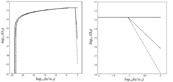
Figure 4.3: Left panel: Evolution of the density parameter $\Omega_{g}$ with the scale factor from the beginning of the radiation era till the present time. The solid line shows the density parameter predicted by the three-stage model (De Sitter inflation, radiation, dust). The dashed and dotted lines depict the density parameter predicted by a four-stage model having a dark energy era right after the dust era with $l=-3,\,-1$, respectively, and $a_{0}/a_{3}=11$. Note that the four-stage model predicts a lower present value for $\Omega_{g}$ than the three-stage one as $\Omega_{g}$ decreases, in a $l$ dependent fashion, during the dark energy era. The right panel is a blow up of the region in which the four-stage models ($l=-3,\,-1$), notably differ from the three-stage one.

By contrast, if a second dust era followed the accelerated (dark energy) era, $\Omega_{g}$ would grow in this second dust era because long wave lengths would continuously be entering that sphere, see Fig. 4.4. This immediately suggests a criterion to be used by future observers to ascertain whether the era they are living in is still our accelerated, dark energy-dominated, era or a subsequent non-accelerated era. By measuring $\Omega_{g}$ at conveniently spaced instants they shall be able to tell. Further, if that era were the accelerated one and the $\Omega_{g}$ measurements were accurate enough they will be able to find out the value of the parameter $l$ occurring in the expansion law given by Eq. (4.1). The lower $l$, the higher the slope of $\Omega_{g}$ in the second dust era.

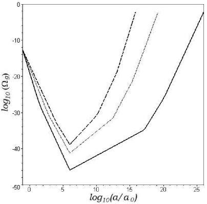
Figure 4.4: Evolution of the density parameter $\Omega_{g}$ given by Eqs. (4.26)-(4.31) with the scale factor in a five-stage scenario (De Sitter inflation-radiation-dust-dark energy-second dust era) from the beginning of the dark energy era. The second dust era starts at the time in which the graphs attain their minimum. The solid, dotted and dashed lines correspond to $l=-1$, $l=-1.5$ and $l=-2$, respectively. The density parameter decreases in the dark energy era and increases in the second dust era till its value is comparable to unity. From that point on our approach (being linear) ceases to apply. We have chosen a dark energy era which begins when $a_{3}/a_{0}=1/11$ and ends when $a_{4}/a_{0}=10^{6}$.

One may argue, however, that these observers may know more easily from supernova data. Nonetheless, if this epoch lies in the faraway future it may well happen that by then the ability of galaxies to generate stars (and hence enough supernovae) has seriously gone down and as a result this prime method might be unavailable or severely impaired. At any rate, even if there were plenty of supernova, the simple gravitational wave method just outlined could still play a complementary role.

4.5 Conclusions

In this chapter we studied the power spectrum and the energy density evolution of the relic gravitational waves generated at the big bang by considering the transitions between successive stages of the Universe expansion. In particular, we considered the effect of the present phase of accelerated expansion as well as a hypothetical second dust phase that may come right after the present one. As it turns out, the power spectrum at the current accelerated era, Eq. (4.10), formally coincides with the power spectrum of the conventional three-stage scenario. As a consequence, measurements of $P(\omega)$ will not directly tell us if the Universe expansion is currently accelerated (as we know from the high redshift supernove data) or non-accelerated. However, the density parameter of the gravitational waves evolves differently during these two phases: it stays constant in the decelerated one and goes down in the accelerated era in a $l$ dependent manner. Therefore, the present value of $\Omega_{g}$ may not only confirm us the current acceleration but also may help determine the value the parameter $l$ -see Fig. 4.3- and hence give us invaluable information about the nature of dark energy.

In the faraway future measurements of $P(\omega)$, if sufficiently accurate, will be able to tell if the Universe is still under accelerated expansion (driven by dark energy) or has entered a hypothetical decelerated phase (second dust era) suggested by different authors [50]. This may also be ascertained by measuring the density parameter of the gravitational waves at different instants to see whether it decreases or increases.

Chapter 5 Gravitational waves entropy and the generalized second law

In this chapter we study the evolution of the entropy associated to the GWs as well as the generalized second law (GSL) of gravitational thermodynamics in the present era of accelerated expansion of the Universe. In spite of the fact that the entropy of matter and relic gravitational waves inside the event horizon diminish, the mentioned law is fulfilled provided the expression for the entropy density of the gravitational waves satisfies a certain condition [57]. Section 5.1 gives the power spectrum of the GWs at the beginning of the present era of accelerated expansion. In section 5.2, the entropy of the GWs is defined and its evolution during that era is found. Finally, in section 5.3 an upper bound on the entropy density of the GWs is obtained by straightforward application of the GSL.

5.1 Gravitational waves in the dark energy era

As explained in the previous chapter, the current era of cosmic acceleration is believed to be dominated by the dark energy. For our purposes in this chapter, we shall assume the Universe is currently dominated by a form of everlasting dark energy of constant $\gamma$ lying in the range $(0,2/3)$ (i.e., phantom energy and cosmological constant dominated universes are excluded). The dependence of the scale factor on the conformal time is formally equal to the scale factor in (4.1), without the second dust era, i.e.,

$$a(\eta)=\left\{\begin{array}[]{lcr}-\frac{1}{H_{1}\eta}&(-\infty<\eta<\eta_{1}<0),&\text{De Sitter era}\\ \frac{1}{H_{1}\eta_{1}^{2}}(\eta-2\eta_{1})&(\eta_{1}<\eta<\eta_{2}),&\text{radiation era}\\ \frac{1}{4H_{1}\eta_{1}^{2}}\frac{(\eta+\eta_{2}-4\eta_{1})^{2}}{\eta_{2}-2\eta_{1}}&(\eta_{2}<\eta<\eta_{3}),&\text{dust era}\\ \left(\frac{l}{2}\right)^{-l}\frac{(\eta_{3}+\eta_{2}-4\eta_{1})^{2-l}}{4H_{1}\eta_{1}^{2}(\eta_{2}-2\eta_{1})}\left(\eta_{l}\right)^{l}&(\eta_{3}<\eta),&\text{dark energy era}\end{array}\right.$$ (5.1)

where $l<-1$, $\eta_{l}=\eta+\frac{l}{2}\left[-\textstyle{2\over{l+1}}\,\eta_{3}+\eta_{2}-4\eta_{1}\right]$. Again, the subindexes $1,2,3$ correspond to sudden transitions from De Sitter era to radiation era, from radiation to dust era, and from dust era to dark energy era, respectively, and $H_{i}$ is the Hubble factor at the instant $\eta=\eta_{i}$. The Hubble factor during the current dark energy era obeys

$$H(\eta)=\left(\frac{a_{3}}{a(\eta)}\right)^{1+\frac{1}{l}}H_{3}.$$ (5.2)

The evolution of the quantity $aH$ in terms of the conformal time $\eta$ is sketched in Fig. 5.1.

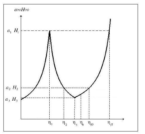
Figure 5.1: Evolution of $a(\eta)H(\eta)$ in a universe with scale factor given by Eq. (5.1).

The modes solution to the gravitational wave equation during the De Sitter era are related with those of the final dark energy era by a Bogoliubov transformation with coefficients $\alpha_{Tr2}$ and $\beta_{Tr2}$, which are formally equal to those found in subsection 4.3.1. At the beginning of the dark energy era, $\eta=\eta_{3}$, the power spectrum was

$$P(\omega)\simeq\left\{\begin{array}[]{ll}0&\left(\omega(\eta_{3})>2\pi(a_{1}/a_{3})H_{1}\right),\\ \\ \frac{1}{4\pi^{2}}\left(\frac{a_{1}}{a_{3}}\right)^{4}H_{1}^{4}\omega^{-1}&\left(2\pi(a_{2}/a_{3})H_{2}<\omega(\eta_{3})<2\pi(a_{1}/a_{3})H_{1}\right),\\ \\ \frac{1}{16\pi^{2}}\left(\frac{a_{3}}{a_{2}}\right)^{2}\left(\frac{a_{1}}{a_{3}}\right)^{8}H_{1}^{6}\omega^{-3}&\left(2\pi H_{3}<\omega(\eta_{3})<2\pi(a_{2}/a_{3})H_{2}\right).\end{array}\right.$$ (5.3)

During the radiation and dust eras $a(\eta)H(\eta)$ decreases with $\eta$ and increases during the De Sitter and dark energy eras. Consequently, as we explained before, GWs are continuously leaving the Hubble radius during the accelerated dark energy era [45, 53]. At some instant $\eta_{f0}$, defined by $a(\eta_{f0})H(\eta_{f0})=a_{2}H_{2}$, the third term in (5.3) ceases to contribute to the power spectrum since the wave lengths of the corresponding GWs exceed the size of the horizon. Finally, at $\eta_{f1}$, defined by $a(\eta_{f1})H(\eta_{f1})=a_{1}H_{1}$, all GWs have their wave length longer than the Hubble radius and the power spectrum vanishes altogether.

5.2 GWs entropy and its evolution in the dark energy era

There are different expressions in the literature for the entropy density of gravitational waves -see e.g., [58, 59, 60]. All of them are based on the assumption that the gravitational entropy is associated with the amount of GWs inside the horizon. In this section, we review the expressions discussed in [59]. Next, we adopt the proposal of Nesteruk and Ottewill [60] to find the evolution to the GWs entropy during the dark energy era.

5.2.1 Entropy of the GWs

Branderberger et al. defined the nonequilibrium entropy of cosmological perturbations in two ways [59]. One of them is based in the microcanonical ensemble [61] while the other is a formula for the entropy that can be associated with the stochastic distribution describing the state of the classical gravitational field. Both descriptions are in agreement.

We shall now summarize the second approach concerning GWs. When the metric perturbations are sufficiently large, the GWs field can be treated as a classical field. The entropy source in this case is the lack of information about the exact field configuration. If a classical field $\varphi(t,\textbf{x})$ and its canonical momentum $\pi(t,\textbf{x})$ are known at all points x at the instant $t$, the state of the system is completely specified and consequently its entropy is zero. But, if all we know about the system is the probability of finding it in a state $\varphi(t,\textbf{x})$, $\pi(t,\textbf{x})$, i.e., $P(\varphi(t,\textbf{x}),\pi(t,\textbf{x}))$, the entropy can be expressed as

$$S=-\int P\left(\varphi(\textbf{x}),\pi(\textbf{x})\right)\;\ln P\left(\varphi(\textbf{x}),\pi(\textbf{x})\right)\;D\varphi(\textbf{x})D\pi(\textbf{x}),$$ (5.4)

where $D\varphi(\textbf{x})D\pi(\textbf{x})$ denotes the functional integral measure for a scalar field.

When the initial state of the system is Gaussian and the time evolution preserves its Gaussian character, the probability distribution $P(\varphi(t,\textbf{x}),\pi(t,\textbf{x}))$ can be expressed in terms of the two point correlations functions $\langle\varphi(t,\textbf{x})\varphi(t,\textbf{y})\rangle$, $\langle\pi(t,\textbf{x}))\pi(t,\textbf{y})\rangle$ and $\langle\varphi(t,\textbf{x})\pi(t,\textbf{y})\rangle$, where $\langle q\rangle$ stands for the ensemble average of $q$ (wich coincides with the space average of $q$ for a spatially homogeneous stochastic process). In this the case, the entropy per unit volume can be expressed as

$$s=\int d^{3}\textbf{k}\ln\left(\langle|\varphi_{k}|^{2}\rangle\langle|\pi_{k}|^{2}\rangle-\langle|\varphi_{k}|^{2}|\pi_{k}|^{2}\rangle\right),$$ (5.5)

where $\varphi_{k}$ and $\pi_{k}$ are the Fourier transformed of $\varphi(t,\textbf{x})$ and $\pi(t,\textbf{x})$ respectively.

The correlation functions of the GWs field can be expressed in terms of the Bogoliubov coefficients (see [59] for more details). Finally, the entropy density reads

$$s=\int d^{3}k\ln N(k),$$ (5.6)

where $N(k)=|\beta_{Tr2}|^{2}$ is the number of GWs created from the initial vacuum with a given wave number $k$. The above expression is valid in the classical limit, i.e., $N(k)\gg 1$.

In [60], Nesteruk and Ottewill proposed a definition of the entropy of GWs based on the idea that the number of generated GWs describes the capacity of the gravitational field to create matter and is associated with the gravitational entropy. Their proposal assume the entropy density is proportional to the GWs number density, i.e.,

$$s_{g}=A\,n_{g}\,,$$ (5.7)

where $n_{g}$ is the number density of gravitational waves, and $A$ is an unknown positive–definite constant of proportionality. We shall now make use of this definition to evaluate the GWs entropy and to study its evolution in the scenario of the previous section.

5.2.2 GWs entropy in the dark energy era

We are interested in the evolution of $n_{g}$ during the dark energy era. The number density of GWs created from the initial vacuum state is

$$dn_{g}(\eta)=\left[\frac{\omega^{2}(\eta)}{2\pi^{2}}d\omega(\eta)\right]|\beta_{Tr2}|^{2}=\frac{P(\omega(\eta))}{2\omega(\eta)}\,d\omega(\eta),$$ (5.8)

where the term in square brackets is the density of states and, as we have seen, $|\beta_{Tr2}|^{2}$ is the number of GWs created. We can obtain $n_{g}(\eta)$ by inserting Eq. (5.3) into Eq. (5.8) and integrating over the frequency.

At the beginning of the dark energy era the GWs number density is

$$n_{g}(\eta_{3})=n_{g}(\eta_{2})\left(\frac{a_{2}}{a_{3}}\right)^{3}+\frac{1}{768\pi^{5}}\left(\frac{a_{1}}{a_{2}}\right)^{2}\left(\frac{a_{2}}{a_{3}}\right)^{3}H_{1}^{3}\left[\left(\frac{a_{3}}{a_{2}}\right)^{\frac{3}{2}}-1\right],$$ (5.9)

where

$$n_{g}(\eta_{2})=\frac{1}{16\pi^{3}}\left(\frac{a_{1}}{a_{2}}\right)^{3}H_{1}^{3}\left[\frac{a_{2}}{a_{1}}-1\right]$$ (5.10)

is the number density at the transition radiation era–dust era.

For $\eta<\eta_{f0}$, i.e. $\frac{a(\eta)}{a_{3}}<\left(\frac{a_{3}}{a_{2}}\right)^{-\frac{l}{2}}$, one has

$$n_{g}(\eta_{3}<\eta<\eta_{f0})=n_{g}(\eta_{2})\left(\frac{a_{2}}{a(\eta)}\right)^{3}+\frac{1}{768\pi^{5}}\left(\frac{a_{1}}{a_{2}}\right)^{2}\left(\frac{a_{2}}{a_{3}}\right)^{3}H_{1}^{3}$$

$$\times\left(\frac{a_{3}}{a(\eta)}\right)^{3}\left[\left(\frac{a_{3}}{a(\eta)}\right)^{-\frac{3}{l}}\left(\frac{a_{3}}{a_{2}}\right)^{\frac{3}{2}}-1\right].\qquad$$ (5.11)

The density number given by Eq. (5.11) decreases with the scale factor because of two effects: $(i)$ the evolution of the volume considered, which grows as $a^{3}$, and $(ii)$ the exit of those waves whose wave length becomes longer than the Hubble radius, which appears in the term in square brackets. As $\frac{a(\eta)}{a_{3}}$ approaches $\left(\frac{a_{3}}{a_{2}}\right)^{-\frac{l}{2}}$, this term tends to zero. From this instant (defined as $\eta_{f0}$) on, the number density reads

$$n_{g}(\eta_{f0}<\eta<\eta_{f1})=\frac{1}{16\pi^{3}}\left(\frac{a_{1}}{a_{3}}\right)^{3}H_{1}^{3}\left(\frac{a_{3}}{a(\eta)}\right)^{3}$$

$$\times\left[\left(\frac{a_{2}}{a_{1}}\right)^{\frac{1}{2}}\left(\frac{a_{3}}{a_{1}}\right)^{\frac{1}{2}}\left(\frac{a_{3}}{a(\eta)}\right)^{-\frac{1}{l}}-1\right].$$ (5.12)

As time goes on, the term in brackets tends to zero and at the instant $\eta_{f1}$, $n_{g}$ vanishes.

Consequently, the entropy density, proportional to the number density, decreases during the dark energy era not just because of the variation of the volume considered but also because of the disappearance of the GWs from the Hubble volume.

The GWs entropy inside the event horizon is

$$S_{g}=\textstyle{4\pi\over{3}}R_{H}^{3}s_{g}\,,$$ (5.13)

where $R_{H}=a(t)\,\int_{t}^{\infty}{dt^{\prime}/a(t^{\prime})}\,$ is the radius of the event horizon and $t$ the cosmic time. For the horizon to exist $R_{H}$ must not diverge. For expansions of the general form $a(\eta)\propto\eta^{l}$ where $l<-1$, the horizon exists and can be expressed as $R_{H}=-lH^{-1}(\eta)$. Since it is of the order of magnitude of the Hubble radius, $H^{-1}$, we will neglect $-l$ and use both terms interchangeably.

Making use of Eq. (5.2) and Eqs. (5.11)-(5.12) , we obtain

$$S_{g}(\eta_{3} < \eta<\eta_{f0})=\frac{4\pi}{3}H_{3}^{-3}A\left(\frac{a_{3}}{a(\eta)}\right)^{-3/l}\left\{n_{g}(\eta_{2})\left(\frac{a_{2}}{a_{3}}\right)^{3}\right.$$ (5.14)

$$\left.+\frac{1}{768\pi^{5}}\left(\frac{a_{1}}{a_{2}}\right)^{2}\left(\frac{a_{2}}{a_{3}}\right)^{3}H_{1}^{3}\left[\left(\frac{a_{3}}{a(\eta)}\right)^{-\frac{3}{l}}\left(\frac{a_{3}}{a_{2}}\right)^{\frac{3}{2}}-1\right]\right\},$$

and

$$S_{g}(\eta_{f0} < \eta<\eta_{f1})=\frac{4\pi}{3}H_{3}^{-3}A\left(\frac{a_{3}}{a(\eta)}\right)^{-3/l}\frac{1}{16\pi^{3}}\left(\frac{a_{1}}{a_{3}}\right)^{3}H_{1}^{3}$$ (5.15)

$$\times\left[\left(\frac{a_{2}}{a_{1}}\right)^{\frac{1}{2}}\left(\frac{a_{3}}{a_{1}}\right)^{\frac{1}{2}}\left(\frac{a_{3}}{a(\eta)}\right)^{-\frac{1}{l}}-1\right].$$

The GWs entropy is a decreasing function of the scale factor and consequently of conformal time. The next section explores whether this entropy descent can be compensated by an increase of the entropy of the other contributors, namely, matter and horizon.

5.3 The generalized second law

In this section, we study the implications the GSL of thermodynamics has over the GWs entropy during the dark energy era.

By extending the GSL of black hole spacetimes [62] to cosmological settings, several authors have considered the interplay between ordinary entropy and the entropy associated to cosmic event horizons [63, 64]. According the GSL of gravitational thermodynamics the entropy of the horizon plus its surroundings (in our case, the entropy in the volume enclosed by the horizon) cannot decrease. Consequently, we must evaluate the total entropy to see its evolution during the present dark energy era.

The cosmological event horizon has an associated entropy that may be interpreted analogously to the entropy of the black hole [65]. An observer living in an accelerated FRW universe has a lack of information about the regions outside its event horizon (see figure 5.2). The area of the horizon, ${\cal A}=4\pi\,H^{-2}$, represents a measure of this lack of information. As in the case of the black hole horizon, we define the entropy of the cosmological horizon as $S_{H}={\cal A}/4$.

Thus, the entropy of the horizon in our case reads

$$S_{H}=\pi H^{-2}(\eta)=\pi H_{3}^{-2}\left(\frac{a_{3}}{a(\eta)}\right)^{-2-\frac{2}{l}},$$ (5.16)

and increases with expansion. (Bear in mind that $l<-1$, i.e., the dark energy behind the acceleration is not of “phantom” type [66]).

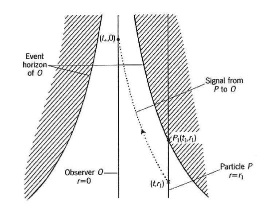
Figure 5.2: The event horizon of an observer in an accelerated FRW universe (a De Sitter universe in this case). The signal emitted by a particle $P$ at the instant $t<t_{1}$ arrives to the observer at the finite instant $t_{*}$. Therefore, as $t\rightarrow t_{1}$, it follows that $t_{*}\rightarrow\infty$ and the light signal takes longer and longer to arrive from the particle to the observer. Signals emitted once the particle is beyond the horizon will never reach the observers position. (Adapted from Fig. $23.5$ of Ref. [67]).

Here we assume that the entropy of the dark energy field responsible for the acceleration does not vary.

The non-relativistic matter fluid entropy must be also considered. If the latter consists in particles of mass $m$ and each of them contributes $k_{B}=1$ to the matter entropy, we get

$$S_{m}=\frac{\rho_{m}}{m}\frac{4\pi}{3}H^{-3}=\frac{H_{3}^{-1}}{2m}\left(\frac{a_{3}}{a(\eta)}\right)^{-\frac{3}{l}},$$ (5.17)

for the entropy of the non-relativistic fluid. Here, we made use of the conservation equation $\rho_{m}(\eta)=\rho_{m}(\eta_{3})\left(\frac{a_{3}}{a(\eta)}\right)^{3}=\frac{3}{8\pi}H_{3}^{2}\left(\frac{a_{3}}{a(\eta)}\right)^{3}$ with $\rho_{m}$ the energy density of matter. From (5.17), it is apparent that $S_{m}$ decreases with expansion.

In virtue of the above equations, the GSL, $S^{\prime}_{m}+S^{\prime}_{g}+S^{\prime}_{H}\geqslant 0$, where the prime indicates derivation with respect to $\eta$, can be written as

$$\frac{3}{l}\left[\frac{H_{3}^{-1}}{2m}+\frac{4\pi}{3}AH_{3}^{-3}\left(\frac{a_{2}}{a_{3}}\right)^{3}n_{g}(\eta_{2})\right]+\left(2+\frac{2}{l}\right)\pi H_{3}^{-2}\left(\frac{a_{3}}{a(\eta)}\right)^{-2+\frac{1}{l}}$$

$$+\frac{3}{l}\frac{A}{576\pi^{4}}\left(\frac{a_{1}}{a_{2}}\right)^{2}\left(\frac{a_{2}}{a_{3}}\right)^{3}H_{1}^{3}H_{3}^{-3}\left[2\left(\frac{a_{3}}{a(\eta)}\right)^{-\frac{3}{l}}\left(\frac{a_{3}}{a_{2}}\right)^{\frac{3}{2}}-1\right]\geqslant 0,$$ (5.18)

for $\frac{a(\eta)}{a_{3}}<\left(\frac{a_{3}}{a_{2}}\right)^{-\frac{l}{2}}$, and

$$\frac{3}{l}\frac{H_{3}^{-1}}{2m}+\left(2+\frac{2}{l}\right)\pi H_{3}^{-2}\left(\frac{a_{3}}{a(\eta)}\right)^{-2+\frac{1}{l}}$$

$$+\frac{3}{l}\frac{A}{12\pi^{2}}\left(\frac{a_{1}}{a_{3}}\right)^{3}H_{1}^{3}H_{3}^{-3}\left[\frac{4}{3}\left(\frac{a_{2}}{a_{1}}\right)^{\frac{1}{2}}\left(\frac{a_{3}}{a_{1}}\right)^{\frac{1}{2}}\left(\frac{a_{3}}{a(\eta)}\right)^{-\frac{1}{l}}-1\right]\geqslant 0,$$ (5.19)

for $\frac{a(\eta)}{a_{3}}>\left(\frac{a_{3}}{a_{2}}\right)^{-\frac{l}{2}}$.

For $l<-1$, both conditions are of the type $f\left(\frac{a(\eta)}{a_{3}}\right)\geqslant 0$, $\,\,f$ being an increasing function of $a(\eta)$. Therefore, if the condition holds true at the beginning of the dark energy era, $\eta=\eta_{3}$, it will hold for $\eta>\eta_{3}$.

By setting $a(\eta)=a_{3}$ in Eq. (5.18), a restriction over the unknown constant $A$ of proportionality follows

$$A\leqslant\frac{-\left(2l+2\right)\frac{\pi}{3}H_{3}-\frac{H_{3}^{2}}{2m}}{\frac{4\pi}{3}\left(\frac{a_{2}}{a_{3}}\right)^{3}n_{g}(\eta_{2})+\frac{1}{576\pi^{4}}\left(\frac{a_{1}}{a_{2}}\right)^{2}\left(\frac{a_{2}}{a_{3}}\right)^{3}H_{1}^{3}\left[2\left(\frac{a_{3}}{a_{2}}\right)^{\frac{3}{2}}-1\right]}\,,$$ (5.20)

implying that for the GSL to be satisfied the above upper bound must be met. In this case the event horizon soon comes to dominate the total entropy and steadily augments with expansion. So, even though the entropy of matter and GWs within the horizon decrease during the present dark energy era, the GSL is preserved provided Eq. (5.20) holds. Note that since the authors of Ref. [60] left the constant $A$ unspecified restriction (5.20) turns to be all the more important: it is the only knowledge we have about how large $A$ may be.

Obviously, our conclusions hang on the expression adopted for the entropy density of the gravitational waves. Here we have chosen (5.7) since, on the one hand, it is the simplest one based on particle production in curved spacetimes [22], and on the other hand, $s_{g}$ cannot fail to be an increasing function of $n_{g}$. We believe, that any sensible expression for $s_{g}$ should not run into conflict with the GSL, and that the latter may impose restrictions on the parameters entering the former.

As mentioned above, we have left aside models of late acceleration driven by dark energy of “phantom type” (i.e., $-1<l<0$) [66]. In this case, owing to the fact that the dominant energy condition is violated, the event horizon decreases with expansion. We shall focus our attention on this issue in the next chapter.

5.4 Conclusions

The number of gravitational waves inside the cosmological event horizon in a four-stage model with scale factor given by (5.1) is a decreasing function of time in the present dark energy era. The GWs entropy in the horizon is associated with the amount of GWs inside it. Consequently, the GWs entropy in the horizon decreases with time.

In order to study the GSL in this scenario, we must consider all the possible contributions to the total entropy: the entropy of the horizon itself (which is proportional to the horizon area and, consequently, it increases with time), the entropy of the dark energy field (which is zero as we assume the field is in a specified state) and the entropy of ordinary matter (which is proportional to the number of particles of ordinary matter present inside the horizon and is a decreasing function of time). If we assume the relation between the GWs entropy and the number of GWs is (5.7), the GSL imposes a bound over the constant $A$ of proportionality.

Chapter 6 The generalized second law in universes dominated by dark energy

In this chapter we leave the main subject of the thesis, the spectrum of GWs, to explore the thermodynamics of dark energy taking into account the existence of the observer s event horizon in accelerated universes. Here we shall not consider GWs as we will focus our attention on one single stage of expansion. Thus, there is no transitions between different stages and no GWs creation.

As we shall see, phantom and non -phantom dark energies satisfy the generalized second law of gravitational thermodynamics whether the equation of state parameter is constant or not. Phantom energy transcends the holographic principle, non–phantom energy complies with it [68].

6.1 Phantom dark energy

As mentioned before, nowadays there is an ample consensus on the observational side that the Universe is undergoing an accelerated expansion likely driven by some unknown fluid, the DE, with the distinguishing feature of violating the strong energy condition, $\rho+3p>0$ [39, 46, 47, 69]. The strength of this acceleration is presently a matter of debate mainly because it depends on the theoretical model employed when interpreting the data. While a model independent analysis suggests it to be below the De Sitter value [70] it is certainly true that the body of observational data allows for a wide parameter space compatible with an acceleration value larger than De Sitter s [66]. If eventually this proves to be the case, the fluid driving the expansion would violate not only the strong energy condition but the dominant energy condition, $\rho+p>0$, as well. In general, fluids of such characteristics, dubbed phantom fluids, face some theoretical difficulties on their own such as quantum instabilities [71]. Nevertheless, phantom models have attracted much interest, among other things because in their barest formulation they predict the Universe to end from an infinite expansion in a finite time ( big rip ), rather than in a big crunch, preceded by the ripping apart of all bound systems, from galaxy clusters down to atomic nuclei [66]. While this scenario might look weird, given our incomplete understanding of the physics below $\rho+p=0$ and the scarcity of reliable observational data, it should not be discarded right away; on the contrary we believe it warrants some further consideration.

Recently, it has been demonstrated that if the expansion of the Universe is dominated by phantom fluid, black holes will decrease their mass and eventually disappear altogether [72]. At first sight this means a threat for the second law of thermodynamics as these collapsed objects are the most entropic entities of our world. This short consideration spurs us to explore the thermodynamic consequences of phantom -dominated universes. In doing so one must take into account that ever accelerating universes have a future event horizon (or cosmological horizon). Since the horizon implies a classically unsurmountable barrier to our ability to see what lies beyond it, it is natural to attach an entropy to the horizon size (i.e., to its area) for it is a measure of our ignorance about what is going on in the other side. However, this has been proved in a rigorous manner for the De Sitter horizon only [65] which, in addition, has a temperature proportional to the Hubble expansion rate. Nevertheless, following previous authors [63, 64, 73] here we conjecture that this also holds true for non-stationary event horizons.

Phantom expansions of pole-like type

$$a(t)\propto\frac{1}{(t_{*}-t)^{n}}\qquad(t\leq t_{*},\;\;0<n=\mbox{constant})\,,$$ (6.1)

as proposed by Caldwell [66], arise when the equation of state parameter $w\equiv p/\rho=\gamma-1=\mbox{constant}<-1$. Current cosmological observations hint that $w$ may be as low as $-1.5$ [39, 47]. In what follows it will be useful to bear in mind that $n=-2/[3(1+w)]>0$.

From the above equation for the scale factor it is seen that the Hubble expansion rate augments

$$H(t)\equiv\frac{\dot{a}}{a}=\frac{n}{t_{*}-t}\,,$$ (6.2)

whereby the radius of the observer’s event horizon

$$R_{H}=a(t)\int_{t}^{\infty}{\frac{dt^{\prime}}{a(t^{\prime})}}=a(t)\int_{t}^{t_{*}}{\frac{dt^{\prime}}{a(t^{\prime})}}=\frac{t_{*}-t}{1+n}=\frac{n}{1+n}H^{-1}\qquad(c=1)\,$$ (6.3)

decreases with time, i.e., $\dot{R}_{H}<0$, and vanishes altogether at the big rip time $t_{*}$. Consequently the horizon entropy,

$$S_{H}=\frac{{\cal A}}{4}=\pi R_{H}^{2},$$ (6.4)

diminishes with time, $\dot{S}_{H}<0$. This is only natural since for spatially flat FRW phantom-dominated universes one has

$$\dot{H}=-4\pi\,(\rho+p)>0,$$ (6.5)

as these fluids violate the dominant energy condition. Then the question arises, “will the generalized second law (GSL) of gravitational thermodynamics, $\dot{S}\,+\,\dot{S}_{H}\geq 0$, be respected?” According to the GSL the entropy of matter plus fields inside the horizon plus the entropy of the event horizon cannot decrease with time. For the interplay between ordinary matter (and radiation) and the cosmological event horizon, see Refs. [57, 63, 64, 73].

6.2 Phantom and non-phantom dark energy with constant $w$

In this section we study the evolution of the phantom DE with constant $w$, next we compare it with the entropy of the non–phantom DE with constant w and, finally, we examine the GSL in both models.

In the previous chapter we assumed that the dark energy has no entropy associated with it, which would be a reasonable choice if the dark energy is given by a scalar field in a pure state. But this is far from being the more natural assumption. Henceforward, we shall see both phantom and non–phantom fluids as phenomenological representations of a mixture of fields, each of which may or may not be in a pure state but the overall (or effective) field is certainly in a mixed state and therefore entitled to have an entropy. This is the case, for instance, of assisted inflation [74].

The entropy of the phantom fluid inside the cosmological event horizon of a comoving observer can be related to its energy and pressure in the horizon by Gibbs equation

$$T\,dS=dE\,+\,p\,d\left(\textstyle{4\over{3}}\pi R_{H}^{3}\right)\,,$$ (6.6)

where owing to the fact that the number of phantom particles inside the horizon is not conserved we have set the chemical potential to zero.From the relation $E=(4\pi/3)\rho R_{H}^{3}$, together with the Friedmann equation $\rho=(3/8\pi)H^{2}$, Eq. (6.3), and the equation of state $p=w\rho$ (with $w<-1$), we get

$$T\,dS=-\frac{n}{1+n}\,dR_{H}.$$ (6.7)

Since $dR_{H}<0$ the phantom entropy increases with expansion (so long as $T>0$).

To proceed further, we must specify the temperature of the phantom fluid. The only temperature scale we have at our disposal is the temperature of the event horizon, which we assume to be given by its De Sitter expression [65]

$$T_{H}=\frac{n}{1+n}\frac{1}{2\pi\,R_{H}}\,,$$ (6.8)

though in our case $\dot{H}\neq 0$. Thus, it is natural to suppose that $T\propto T_{H}$ and then figure out the proportionality constant. As we shall see below, this choice is backed by the realization that it is in keeping with the holographic principle [75]. The simplest choice is to take the proportionality constant as unity which means thermal equilibrium with the event horizon, $T=T_{H}$. Otherwise energy would spontaneously flow between the horizon and the fluid (or viceversa), something at variance with the FRW geometry. Note that, explicitly or implicitly, every FRW model (including inflation models) assumes thermal equilibrium.

After integration of Eq. (6.7), bearing in mind that $S\rightarrow 0$ as $t\rightarrow t_{*}$, the entropy of the phantom fluid can be written as $S=-{\cal A}/4$.

Some consequences follow: $(i)$ The phantom entropy is a negative quantity, something already noted by other authors [76], and equals to minus the entropy of a black hole of radius $R_{H}$. $(ii)$ It bears no explicit dependence on $w$ and, but for the sign, it exactly coincides with the entropy of the cosmological event horizon. $(iii)$ Since $-S\propto E^{2}$ it is not an extensive quantity. Note that $S$ does not scale with the volume of the horizon but with its area. One may argue that the first consequence was to be expected since (for $T>0$) it readily follows from Euler’s equation $T\,s=\rho+P$, $s$ being the entropy density. However, it is very doubtful that Euler’s equation holds for phantom fluids since it is based on the extensive character of the entropy of the system under consideration [77] and we have just argued that for phantom fluids this is not the case. The fact that $S<0$ tells us that the entropy of the phantom fluid is not to be understood as a measure of the number of microstates associated to the macroscopic state of the fluid and that, in general, the current formulation of statistical mechanics might not apply to systems that violate the dominant energy condition. Before closing this paragraph, it is noteworthy that negative entropies are not so new after all; in principle monoatomic ideal gases may exhibit such a feature for sufficiently low temperatures [78].

Two further consequences are: $(iv)$ The sum $S+S_{H}$ vanishes at any time, therefore the GSL is not violated -the increase of the (negative) phantom entropy exactly offsets the entropy decline of the event horizon. $(v)$ $\mid S\mid$ saturates the bound imposed by the holographic principle [75]. The latter asserts that the total entropy of a system enclosed by a spherical surface cannot be larger than a quarter of the area of that surface measured in Planck units. (For papers dealing with the holographic principle in relation with dark energy, see [79] and references therein). In this connection, it is interesting to see that if the equation of state were such the entropy obeyed $S^{*}=\varkappa\,S$, with $\varkappa$ a positive–definite constant, then the GSL would impose $1\leq\varkappa$. This leads us to conjecture that the entropy of phantom energy is not bounded from below but from above, being $-S_{H}$ its upper limit.

Nevertheless, in a less idealized cosmology one should consider the presence of other forms of energy, in particular of black holes and the decrease in entropy of these objects [72]. It is unclear whether in such scenario the GSL would still hold its ground. Nonetheless, one may take the view that the GSL may impose an upper bound to the entropy stored in the form of black holes. At any rate, the calculation would be much more involved and we leave it to a future research. Among other things, one should take into account that the scale factor would not obey such a simple expansion law as (6.1) and that the black holes would be evaporating via Hawking radiation [32] which would also modify the expansion rate and, accordingly, the horizon size.

A straightforward and parallel study for a non–phantom dark energy-dominated universe with constant parameter of state (lying in the range $-1<w<-1/3$), shows that in this case too $\dot{S}+\dot{S}_{H}=0$. There are two main differences, however; on the one hand the entropy of the fluid decreases while the area of event horizon augments, and on the other hand $S\geq 0$. The latter comes from adopting the view that the dark energy must vanish for $T\rightarrow 0$ (Planck’s statement of the third law of thermodynamics) and realizing that this happens for $t\rightarrow\infty$. Again, $S$ saturates the bound imposed by the holographic principle.

Another important difference between phantom and non–phantom dark–energy expansions is that while the former gets hotter and hotter the latter gets colder and colder. This implies the following. As the phantom fluid heats up its ability to produce black holes via quantum tunnelling may augment and the probability for this to occur becomes high near the Planck limit [30]. This is a very strongly irreversible process since the variation of entropy is enormous going from negative values (phantom fluid) to positive values (black holes). Obviously, the black hole production would severely alter the dynamics of the last stage of expansion. Two competing effects come into play, namely: the tendency to produce black holes via tunnelling, and the tendency to destroy these black holes via the Babichev effect [72] (also the tendency of the black holes to evaporate may play a non–negligible role). Depending on which one of these eventually comes to dominate two rather different scenarios arise: $(i)$ If the Babichev effect dominates, the play will be rehearsed again and again, probably never reaching the big rip ($t=t_{*}$) but the Universe will always be accelerating. $(ii)$ If the quantum tunnelling process takes the upper hand, the Universe will exit the phantom regime and come back to the old Einstein-De Sitter expansion during the time taken by the black hole to evaporate into radiation. This achieved, the universe will start a new radiation dominated era. As a consequence the analysis of above will be found inconsistent as a whole because if the Universe is to resume a non–accelerating regime no cosmological event horizon would have ever existed.

Coming back to the phantom energy discussion, one may adopt the point of view that the phantom temperature is negative [80]. But, as mentioned above, this would destroy the FRW geometry. On the other hand, negative temperatures are linked to condensed matter systems whose energy spectrum is bounded from above and may therefore exhibit the phenomenon of population inversion, i.e., their upper energy states can be found more populated than their lower energy states [81]. However, all models of phantom energy proposed so far consist in some or other type of scalar field with no upper bound on their energy spectrum. In addition, while population inversion is a rather transient phenomenon the phantom regime is supposed to last for cosmological times. Moreover, bearing in mind that $w<-1$ and $dR_{H}<0$, it follows from Eq. (6.7) that if $T$ were negative, then the phantom entropy would decrease with expansion and the GSL would be violated.

6.3 Phantom and non–phantom dark energy with variable $w$

One may argue that the result $\dot{S}+\dot{S}_{H}=0$ critically depends on the particular choice of the equation of state parameter $w$ to the point that if it were not constant, then the GSL could be violated. Here we shall explore this issue taking the phantom model with $w$ dependent on time of Sami and Toporensky [82].

In this model a scalar field, $\phi(t)$, with negative kinetic energy, minimally coupled to gravity sources with energy density and pressure given by

$$\rho=-\frac{{\overset{.}{\phi}}^{2}(t)}{2}+V(\phi),\text{\qquad}p=-\frac{{\overset{.}{\phi}}^{2}(t)}{2}-V(\phi),$$

respectively, is adopted. The equation of state parameter

$$w=\frac{p}{\rho}=\frac{\frac{\overset{.}{\phi}^{2}(t)}{2}+V(\phi)}{\frac{\overset{.}{\phi}^{2}(t)}{2}-V(\phi)},$$

is lower than $-1$ as long as $\rho$ is positive and depends on time.

When the kinetic energy term is subdominant (“slow climb” [82]) the evolution equation of the phantom field simplifies to

$$3H\overset{.}{\phi}(t)\simeq\frac{dV(\phi)}{d\phi}.\text{\qquad}$$ (6.9)

Assuming also the power law potential $V(\phi)=V_{0}\,\phi^{\alpha}$ with $\alpha$ a constant, restricted to the interval $0<\alpha\leq 4$ to evade the big rip, the equation of state parameter reduces to $w\simeq-1-\frac{\alpha}{6x}$, where $x=2\pi\,\phi^{2}$ is a dimensionless variable, and the field is an ever increasing function of time, namely,

$$\phi(t) = \left[\phi_{i}^{\frac{4-\alpha}{2}}+\sqrt{\frac{V_{0}}{24\pi}}\,\frac{\left(4-\alpha\right)\alpha}{2}\left(t-t_{i}\right)\right]^{\frac{2}{4-\alpha}}\quad(0<\alpha<4),$$ (6.10)

$$\phi(t) = \phi_{i}\,\exp\left[4\sqrt{\frac{V_{0}}{24\pi}}\,(t-t_{i})\right]\qquad(\alpha=4),$$ (6.11)

where the subscript $i$ stands for the time at which the phantom energy begins to dominate the expansion. Thus $w$ increases with expansion up to the asymptotic value $-1$. Likewise the scale function obeys

$$a(\phi)=a_{i}\,\exp\left[\frac{4\pi}{\alpha}\,(\phi^{2}-\phi_{i}^{2})\right]\,.$$ (6.12)

As it should, the Hubble factor

$$H=\sqrt{\frac{2V_{0}}{3}}\,\left(4\pi\right)^{\frac{1}{2}-\frac{\alpha}{4}}\alpha^{\alpha/4}\,x^{\alpha/4}$$ (6.13)

augments with expansion while the cosmological event horizon

$$R_{H}=x^{\alpha/4}\,\Gamma\left(1-\frac{\alpha}{4},x\right)\,\frac{e^{x}}{H}$$ (6.14)

decreases monotonically to vanish asymptotically -see Figure 6.1. Here $\Gamma\left(\frac{4-\alpha}{4},x\right)$ is the incomplete Gamma function [36].

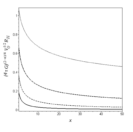
Figure 6.1: Radius of the event horizon vs $x$ for $\alpha=$ $1$, $2$, $3$ and $4$ from top to bottom. In all the cases $R_{H}\rightarrow 0$ as $t\rightarrow\infty$. For convenience sake we have set $x_{i}=1$.

As in the preceding section, the entropy of this phantom fluid can be obtained by using Gibbs’s equation and $T=T_{H}=H/2\pi$. Again, we get a negative quantity that increases with time

$$S=-\pi\,C^{2}\,\int_{x}^{\infty}{}\Gamma^{2}\left(1-\frac{\alpha}{4},\,x\right)\,\frac{\alpha}{2x}\,e^{2x}\,dx\,,$$ (6.15)

here $C=\sqrt{3/(2V_{0})}\,(4\pi)^{-\frac{1}{2}+\frac{\alpha}{4}}\,\alpha^{-\alpha/4}$.

From the above expressions, it follows that

$$\dot{S}+\dot{S}_{H}=\pi\,C\,\left[\Gamma\left(\frac{4-\alpha}{4},\,x\right)\,e^{x}(2+\frac{\alpha}{2x})-2x^{-\alpha/4}\right]\,R_{H}\,\dot{x}\,.$$ (6.16)

Since the quantity in square brackets is positive–definite for any finite $x$ and $\dot{x}>0$, the GSL in the form $\dot{S}+\dot{S}_{H}\geq 0$ is satisfied. The equality sign occurs just for $t\rightarrow\infty$, i.e., when $R_{H}$ vanishes.

As Fig. 6.2 illustrates, the holographic principle is again transcended in the sense that $-\infty<S\leq-S_{H}$.

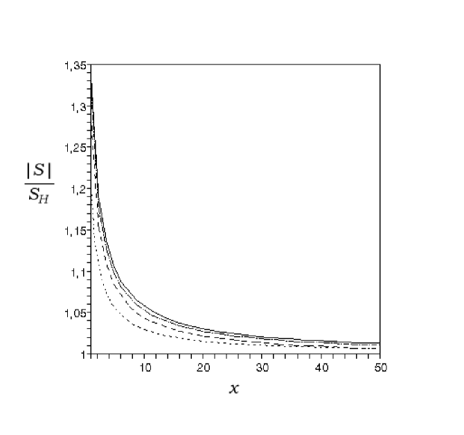
Figure 6.2: Evolution of the ratio between the absolute value of the phantom entropy and the horizon entropy for the model of Ref. [82]. The graphs correspond successively to $\alpha$ values $1$, $2$, $3$, and $4$ from bottom to top. For convenience sake we have set $x_{i}=1$ in drawing the graphs. All the curves asymptote to $x$ = 1.

As an example of non-phantom dark energy with variable $w$ we consider the Chaplygin gas [83]. This fluid is characterized by the equation of state $p=-A/\rho$. Integration of the energy conservation equation yields $\rho=\sqrt{A+(B/a^{6})}$, whereby $w=-A\,a^{6}/(A\,a^{6}\,+B)$. Here $a$ is the scale factor normalized to its present value and $A$ and $B$ denote positive–definite constants. Accordingly, this fluid interpolates between cold matter, for large redshift, and a cosmological constant, for small redshift. This has led to propose it as a candidate to unify dark matter and dark energy [84].

The radius of the cosmological event horizon reads

$$R_{H}=\sqrt{\frac{8\pi}{3}}\,\frac{2}{A^{1/4}}\,x^{1/6}\,\left[1.4712-x^{1/12}\,\,_{2}F_{1}\left(\frac{1}{12},\frac{1}{4},\frac{13}{12};-x\right)\right]\,,$$ (6.17)

where ${}_{2}F_{1}$ is the hypergeometric function and $x=A\,a^{6}/B$ is a dimensionless variable. As figure 6.3 illustrates, $\mbox{Lim}_{\,x\rightarrow\infty}\,R_{H}=\sqrt{3/(8\pi)}\,A^{-1/4}$ which is nothing but the value taken by $H^{-1}$ in that limit. This was to be expected: for large scale factor the Chaplygin gas expansion goes over De Sitter’s.

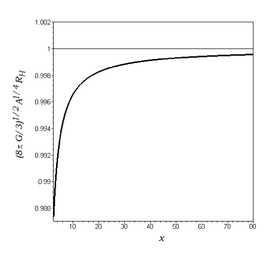
Figure 6.3: Evolution of the adimensionalized radius of the event horizon in the Chaplygin gas model. It tends to unity for $x\rightarrow\infty$.

The horizon temperature is

$$T_{H}=\sqrt{\frac{8\pi}{3}}\,\frac{A^{1/4}}{2\pi}\,\left(\frac{1+x}{x}\right)^{1/4},$$ (6.18)

while the entropy of the fluid and the entropy of the horizon evolve as

$$dS=-\frac{3}{4\,A^{1/2}}\,\frac{1}{x^{2/3}(1+x)}\left[1.4712-x^{1/2}\,\,_{2}F_{1}\left(\frac{1}{12},\frac{1}{4},\frac{13}{12};-x\right)\right]^{2}\,dx\,,$$ (6.19)

and

$$dS_{H}=\frac{1}{4\,A^{1/2}}\,x^{1/6}\,\left[1.4712-x^{1/2}\,\,_{2}F_{1}\left(\frac{1}{12},\frac{1}{4},\frac{13}{12};-x\right)\right]$$ (6.20)

$$\times\left\{2x^{-5/6}\left[1.4712-x^{1/2}\,\,_{2}F_{1}\left(\frac{1}{12},\frac{1}{4},\frac{13}{12};-x\right)\right]-\frac{1}{x^{3/4}\,(1+x)^{1/4}}\right\}\,,$$

respectively. The two latter equation imply that $\dot{S}\,+\,\dot{S}_{H}\geq 0$ for $x\geq 2.509$ or equivalently, for $\rho_{f(i)}\leq 1.18A^{1/2}$. Thus there is an early period in which the GSL seems to fail. However, this may be seen not as a failure of the GSL but as an upper bound on the initial value of the energy density of the Chaplygin gas. This is somewhat similar to the bound imposed on the initial entropy of relic gravitational waves in a universe dominated by non–phantom dark energy [57].

Notice that, $S$ is a positive, ever–decreasing function of the scale factor that complies with the holographic bound $S\leq S_{H}$.

6.4 Quasi-duality between phantom and non-phantom thermodynamics

The duality transformation

$$\left\{\begin{array}[]{ll}H&\rightarrow\overline{H}=-H\\ \rho+p&\rightarrow\overline{\rho}+\overline{p}=-(\rho+p)\end{array}\right.$$ (6.21)

leaves the Einstein’s equations

$$\begin{array}[]{ll}H^{2}=\frac{8\pi}{3}\rho,&\\ \dot{\rho}+3H(\rho+p)=0,&\\ \dot{H}=-4\pi(\rho+p),&\end{array}$$ (6.22)

of spatial FRW universes invariant and the scale factor transforms as $a\rightarrow\overline{a}=1/a$ [85]. Thus, a phantom DE dominated universe with scale factor $a=1/(-t)^{n}$ (for simplicity we assume a phantom scale factor as Eq. (6.1) with $t_{*}=0$ and $t<0$ that tends to $0^{-}$) becomes a contracting universe whose scale factor obeys $\overline{a}=(-t)^{n}$. This universe begins contracting from an infinite expansion at the infinite past and collapses to a vanishing scale factor for $t=0^{-}$ (left panel of Fig. 6.4).

Reversing the direction of time (i.e., the future of $t$, $t+dt$, transforms into $t-dt$), the contracting universe is mapped into an expanding one whose scale factor grows with no bound as $t$ tends to $-\infty$. Notice that the first transformation takes the universe from expanding to contracting and the second transformation makes the universe expand again, i.e., the final cosmology has $\overline{H}>0$. It should be remarked that the latter transformation also preserve Eqs. (LABEL:einsteinequations).

Under this two successive operations, the final and the initial equation of states parameters are related by $w\rightarrow\overline{w}=-(w+2)$. Consequently, phantom DE dominated universes with $n>1$, (i.e., $-5/3<w<-1$) are mapped into non-phantom DE universes (see Fig. 6.4). Therefore, both of them, the original and the transformed universes, have an event horizon and entropies whose relation we derive below.

The radius of the event horizon of the original universe is $R_{H}=(-t)/(1+n)$ meanwhile the radius of the event horizon of the transformed universe is $\overline{R}_{H}=(-t)/(n-1)=R_{H}[(1+n)/(1-n)]$. The transformations preserve the horizon temperature as the Hubble factor does not change. From the definition of the horizon, it is readily seen that

$$\frac{dR_{H}}{dt}=HR_{H}-1.$$ (6.23)

In virtue of the above expression together with the Gibbs equation one obtains

$$T\frac{dS}{dt}=-4\pi(\rho+p)R_{H}^{2},$$ (6.24)

whereby, the entropy transforms as [68]

$$S\rightarrow\overline{S}=-[(1+3w)/(5+3w)]^{2}S.$$ (6.25)

Therefore, the entropy of the final non-phantom dark energy dominated universe is proportional, but of the opposite the sign, to the entropy of the original phantom universe. We might say that the duality transformation “quasi” preserves the thermodynamics of dark energy. This result is in keeping with the findings of Section 6.2.

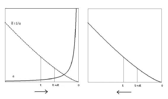
Figure 6.4: The left panel depicts the scale factor of the original phantom dominated universe (solid line). The dashed line shows the evolution of the scale factor dual of this phantom DE model, a contracting universe. In both models (the phantom and its dual) the time grows from left to right as tends to $t=0^{-}$ and the instant $t+dt$ lies at the future of the instant $t$. In the right panel, the time direction is reversed ($t+dt$ lies at the past of $t$). Under this operation, the contracting model of the left panel becomes the non-phantom DE dominated universe of the right panel if $-5/3<w<-1$.

6.5 Conclusions

We explored some thermodynamical consequences for the dark energy when the entropy of the cosmological event horizon is not ignored. Irrespective of if $w$ is constant or not, we have found that phantom fluids possess negative entropy, transcend the holographic bound and their temperature and entropy increase as the Universe expands. By contrast, non-phantom fluids have positive entropy, satisfy the holographic bound and their temperature and entropy decrease with expansion. In all the cases, the GSL is fulfilled.

It goes without saying that negative entropies are hard to assimilate; especially because the Einstein-Boltzmann interpretation of entropy as a measure of the probability breaks down under such circumstances. Systems of negative entropy appear to lie outside the province of statistical mechanics as is currently formulated [81, 86]. Nevertheless, the laws of thermodynamics alone do not entail that S must be a positive quantity. The latter will be found to be positive or negative only after combining these laws with the equation (or equations) of state of the system under consideration. What we believe to be at the core of thermodynamics is the law that forbids the entropy of isolated systems to decrease, this law contains the GSL for gravitating systems with a horizon.

As pointed out by Nojiri and Odintsov, it may well happen that in the last stages of phantom dominated universes the scalar curvature grows enough for quantum effects to play a non-negligible role before the big rip. If so, the latter may be evaded or at least softened [87]. While our study does not incorporate such effects they should not essentially alter our conclusions so long as the cosmic horizon persists.

It is noteworthy that the duality transformation $\rho+p\rightarrow-(\rho+p)$ and $H\rightarrow-H$ along with reversing the direction of time (i.e., $dt\rightarrow-dt$) leaves Einstein’s equations invariant and maps phantom cosmologies, with both $H$ and $\dot{H}$ positive, into non-phantom cosmologies with $H>0$ but $\dot{H}<0$ -see, e.g., [85]. However, this duality does not necessarily extend to the thermodynamics of the respective universes since future event horizons exist only when $\ddot{a}>0$. Nevertheless, in the particular case of pole-like expansions, Eq. (6.1), the transformation preserves the temperature while the entropy transforms as $S\rightarrow-[(1+3w)/(5+3w)]^{2}\,S$ with the constraint $-5/3<w<-1$.

Summary

Cosmology has for a long time been a rather speculative science. Hubble’s discovery that the Universe is expanding, and -more recently- the realization that at present this expansion is accelerated, the measured abundance of light elements, the mass distribution of galaxies and clusters thereof, and the discovery and posterior measurements of the anisotropies of the CMB have changed this picture. Hopefully, measurements of GWs will soon be added to this short list. At any rate, now we can speak confidently of physical cosmology as a fully–fledged branch of Science.

The relic GWs constitute a privileged window to determine the evolution of the Universe. Little is known from the early evolution of the Universe and the predictions for their spectrum depend on the model considered. According to these predictions, a spectrum of relic GWs is generated making feasible its detection with the technology currently being developed.

In this thesis, using the adiabatic vacuum approximation, we have reviewed how the expansion of the Universe amplifies the quantum vacuum fluctuations, and how the relic GWs spectrum is related with the scale factor.

We have later evaluated the spectrum in a four-stage model (which consist on a De Sitter stage, a stage dominated by a mixture of MBHs and radiation, a radiation dominated stage and finally a non-relativistic matter (dust) dominated stage). We have demonstrated that the spectrum in this scenario is much lower than the predicted by three–stage model (De Sitter-radiation era-dust era). We have also shown how the bound over the GWs spectrum from the measured CMB anisotropies places severe constraints over the free parameters of the four-stage model.

We have also considered a scenario featuring an accelerated expanding era dominated by dark energy, right after the dust era of the three–stage model. We have found that the current power spectrum of this four–stage scenario exactly coincides with that of the three–stage, but it evolves in a different fashion. We have considered as well the possibility that the dark energy decays in non–relativistic matter leading to a second dust era in the far future and obtained the power spectrum of the GWs as well as the evolution of the density parameter.

We have applied the generalized second law of thermodynamics to the four–stage model of above. Assuming the GWs entropy proportional to the number of GWs, we have found the GSL is fulfilled provided a certain proportionality constant does not exceed a given upper bound.

Finally, we have extended the GSL study to a single stage universe model dominated by dark energy (either phantom or not), and found that the GSL is satisfied and that the entropy of the phantom fluid is negative. Likewise, we have found a transformation between phantom and non–phantom scenarios preserving the Einstein field equations that entails a “quasi” duality between the thermodynamics of both scenarios.

Appendix A Sudden transition approximation

Let us assume a spatially flat FRW universe which gradually evolves from an initial stage (whose expansion is dominated by a barotropic fluid of index $\gamma_{(r-1)}$) to a next stage dominated by another perfect fluid of barotropic index $\gamma_{r}$. If the transition between both stages begins at the instant $\eta^{-}=\eta_{i}-\Delta\eta_{i}$ and ends at $\eta^{+}=\eta_{i}+\Delta\eta_{i}$, the scale factor as a function of time in this scenario reads

$$a(\eta)=\left\{\begin{array}[]{lr}a_{i-1}\left(\frac{a_{i-1}H_{i-1}}{l_{(r-1)}}\right)^{l_{(r-1)}}\left(\eta-\eta_{i-1}+\frac{l_{(r-1)}}{a_{i-1}H_{i-1}}\right)^{l_{(r-1)}},&\left(\eta_{i-1}<\eta<\eta^{-}\right),\\ a_{tr}(\eta),&\left(\eta^{-}<\eta<\eta^{+},\right),\\ a_{+}\left(\frac{a_{+}H_{+}}{l}\right)^{l_{r}}\left(\eta-\eta^{+}+\frac{l_{r}}{a_{+}H_{+}}\right)^{l_{r}},&\left(\eta^{+}<\eta\right),\end{array}\right.$$ (A.1)

where the subindex $i-1$ denotes the instant when the expansions begins and the subindex $+$ denotes the quantities evaluated at $\eta_{+}$. The function $a_{tr}(\eta)$ describes the smooth transition from one stage to the other. Consequently, in this scenario $a(\eta)$ and $a^{\prime}(\eta)$ are continuous functions of time at the points $\eta_{-}$ and $\eta_{+}$.

The solution to equation (2.10) is

$$\mu_{l_{(r-1)}}(\eta)=\left\{\begin{array}[]{lr}(\sqrt{\pi}/2)e^{i\psi_{l_{(r-1)}}}k^{-1/2}x_{l_{(r-1)}}^{1/2}H_{l_{(r-1)}-\frac{1}{2}}^{(2)}(x_{l_{(r-1)}}),&\left(\eta_{i-1}<\eta<\eta^{-}\right),\\ \mu_{tr}(\eta),&\left(\eta^{-}<\eta<\eta^{+},\right),\\ \alpha_{i}\mu_{l_{r}}(\eta)+\beta_{i}\mu_{l_{r}}^{\ast}(\eta),&\left(\eta^{+}<\eta\right),\end{array}\right.$$ (A.2)

but also

$$\mu_{l_{r}}(\eta)=\left\{\begin{array}[]{lr}\alpha_{i}^{*}\mu_{l_{(r-1)}}(\eta)-\beta_{i}\mu_{l_{(r-1)}}^{\ast}(\eta),&\left(\eta_{i-1}<\eta<\eta^{-}\right),\\ \overline{\mu}_{tr}(\eta),&\left(\eta^{-}<\eta<\eta^{+},\right),\\ (\sqrt{\pi}/2)e^{i\psi_{l_{r}}}k^{-1/2}x_{l_{r}}^{1/2}H_{l_{r}-\frac{1}{2}}^{(2)}(x_{l_{r}}),&\left(\eta^{+}<\eta\right),\end{array}\right.$$ (A.3)

where the solutions in the transition region $\mu_{tr}$ and $\overline{\mu}_{tr}$ are some unknown functions.

By imposing the continuity of $\mu_{l_{(r-1)}}$ and $\mu_{l_{r}}$ and its first derivatives at $\eta^{-}$ and $\eta^{+}$, we get

$$\begin{array}[]{l}\alpha_{i}=i\left[\mu_{tr}^{\prime}(\eta^{+})\mu_{l_{r}}^{*}(\eta^{+})-\mu_{tr}(\eta^{+}){\mu_{l_{r}}^{*}}^{\prime}(\eta^{+})\right]\\ \;\;\;\;\,=i\left[\mu_{l_{r-1}}^{\prime}(\eta^{-})\overline{\mu}_{tr}^{*}(\eta^{-})-\mu_{l_{r-1}}(\eta^{-}){\overline{\mu}_{tr}^{*}}^{\prime}(\eta^{-})\right],\end{array}$$ (A.4)

$$\begin{array}[]{l}\beta_{i}=i\left[\mu_{tr}(\eta^{+})\mu_{l_{r}}^{\prime}(\eta^{+})-\mu_{tr}^{\prime}(\eta^{+})\mu_{l_{r}}(\eta^{+})\right]\\ \;\;\;\;\,=i\left[\mu_{l_{r-1}}(\eta^{-})\overline{\mu}_{tr}^{\prime}(\eta^{-})-\mu_{l_{r-1}}^{\prime}(\eta^{-})\overline{\mu}_{tr}(\eta^{-})\right].\end{array}$$ (A.5)

For modes whose period is much larger than the duration of the transition era (i.e., those modes allowed by the adiabatic vacuum bound $\omega(\eta)<\omega_{i}(\eta)$), the transition can be assumed instantaneous. This is the so-called “sudden transition approximation”. In this limit, we can safely let $\eta^{-}\rightarrow\eta^{+}$. Relabelling the instant $\eta^{+}$ as $\eta_{i}$, we have that $\mu_{tr}(\eta_{i})=\mu_{l_{(r-1)}}(\eta_{i})$, $\overline{\mu}_{tr}(\eta_{i})=\mu_{l_{r}}(\eta_{i})$, and a similar relation for the derivatives evaluated at $\eta_{i}$. Equations (2.41) and (2.42) readily follow from (A.4) and (A.5) in this approximation.

Bibliography

- [1] B. Allen, in Proceedings of the Les Houches School on Astrophysical Sources of Gravitational Waves, edited by J. Marck and J. Lasota (Cambridge University Press, Cambridge, 1996), gr-qc/9604033.
-
[2]
Ch. Misner, Nature 214, 40 (1967);
S.W. Hawking, Astrophys. J. 145, 544 (1966);
V. Méndez, D. Pavón and J.M. salim, Class. Quantum Grav. 14, 177 (1997). - [3] R. A. Hulse and J. H. Taylor, Astrophys. J. Lett. 195, L51 (1975); J. M. Weisberg and J. H. Taylor, Gen. Rel. Grav. 13, 1 (1981).
- [4] C. M. Will, “The Confrontation between General Relativity and Experiment”, Living Rev. Relativity 4, (2001), http://www.livingreviews.org/Articles/Volume4/2001-4will/
- [5] M. Kramer et al., Proceedings of The 22nd Texas Symposium on Relativistic Astrophysics, Stanford University,, astro-ph/0503386.
- [6] S. Rowan and J. Hough, “Gravitational Wave Detection by Interferometry (Ground and Space)”, Living Rev. Relativity 3, (2000), http://relativity.livingreviews.org/Articles/lrr-2000-3
- [7] P. Astone et al., Class. Quantum Grav. 19, 5449 (2002).
- [8] http://tamago.mtk.nao.ac.jp
- [9] http://www.geo600.uni-hannover.de
- [10] http://www.virgo.infn.it
- [11] http://www.ligo.caltech.edu
- [12] http://lisa.jpl.nasa.gov
- [13] J. Crowder and N.J. Cornish, gr-qc/0506015.
- [14] A. Buonanno, TASI lectures on gravitational waves from the early Universe, gr-qc/0303085.
- [15] W. De Sitter, Nature 128, 706 (1931).
- [16] A. Einstein, Preuss. Akad. Wiss. Berlin, Sitzber, 688 (1916).
- [17] E. Lifshitz, J. Phys. USSR 10, 116 (1946).
- [18] L.P. Grishchuk, Class. Quantum Grav. 10, 2449 (1993).
- [19] J. Barrow, J. Mimoso and M.R. de Garcia Maia, Phys. Rev. D 48, 3630 (1994).
- [20] L.P. Grishchuk, Annals N. Y. Acad. Sci. 302, 439 (1977).
- [21] L.P. Grishchuk, Zh. Eksp. Teor. Fiz. 67, 825 (1975) [Sov. Phys. JETP 40, 409 (1975)].
- [22] N.D. Birrell and P.C.W. Davies, Quantum Fields in Curved Space (Cambridge University Press, 1982).
- [23] S.A. Fulling, Aspects of Quantum Field Theory in Curved Space-Time(Cambridge University Press, 1989).
- [24] M.R. de Garcia Maia, Phys. Rev. D 48, 647 (1993).
- [25] M.R. de Garcia Maia, Thesis: “The Stochastic Background of Gravitational Waves” (University of Sussex, 1994).
- [26] G. Izquierdo and D. Pavón, Phys. Rev D 68, 124005 (2003).
- [27] B. Allen, Phys. Rev. D 37, 2078 (1987).
- [28] L.P. Grishchuk, Phys. Rev. D 48, 3513 (1993).
- [29] A.A. Starobinsky, Pis’ma Zh. Eksp. Teor. Fiz. 30, 719 (1979) [JETP Lett. 30, 682 (1980)].
- [30] D. Gross, M.J. Perry and G.L. Yaffe, Phys. Rev. D 25, 330 (1982); J.I. Kapusta, Phys. Rev. D 30, 831 (1984).
- [31] G. Hayward and D. Pavón, Phys. Rev. D 40, 1748 (1989).
- [32] S.W. Hawking, Nature 248, 30 (1974), Comm. Math. Phys., 43, 199 (1975).
- [33] K.S. Thorne, R.H. Price and D.A. Macdonald, Black Holes: The Membrane Paradigm (Yale University Press, 1986).
- [34] J.D. Barrow, E.J. Copeland and A.R. Liddle, Mon. Not. R. Astr. Soc. 253, 675 (1991).
- [35] D. Lindley, Monthly Not. R. Astro. Soc. 196, 317 (1981).
- [36] M. Abramowitz and I.A. Stegun, eds., Handbook of Mathematical Functions (Dover, New York, 1972).
- [37] J. Khoury, B.A. Ovrut, P.J. Steinhardt, N. Turok , Phys. Rev. D 64, 123522 (2001).
- [38] P.J.E. Peebles, Principles of Physical Cosmology (Princeton University Press, Princeton, 1993); T. Padmanabham, Structure Formation in the Universe (Cambridge University Press, Cambridge, 1993).
- [39] D.N. Spergel et al., Astrophys. J. Suppl. 148, 175 (2003).
- [40] S.E. Thorsett and R.J. Dewey, Phys. Rev. D 53, 3468 (1996).
- [41] G. Hinshaw et al., Astrophys. J. Suppl. 148, 135 (2003).
- [42] R.K. Sachs, A.M. Wolfe, Astrophys. J. 147, 73 (1967).
- [43] J.A. Peacock, Cosmological Physics (Cambridge University Press, Cambridge, 1993).
- [44] B. Allen and S. Koranda, Phys. Rev. D 50, 3713 (1994).
- [45] G. Izquierdo and D. Pavón, Phys. Rev. D 70, 084034 (2004).
- [46] Proceedings of the I.A.P. Conference “On the Nature of Dark Energy”, Paris 2002, edited by P. Brax, J. Martin and J.P. Uzan (Frontier Group, Paris, 2002); S.M. Carroll, “Why is the Universe Accelerating” in Measuring and Modeling the Universe (Cambridge University Press, Cambridge, 2004); V. Sahni, Class. Quantum Grav. 19, 3435 (2002); T. Padmanabhan, Phys. Reports 380, 325 (2003); V. Sahni, in Proceedings of the Second Aegean Summer School on the Early Universe, Syros, Greece, 2003, astro-ph/0403324.
- [47] A. Riess et al., Astron. J. 116, 1009 (1998); P. Garnavich et al., Astrophys. J. 509, 74 (1998); S. Perlmutter et al., Astrophys. J. 517, 565 (1999); R.A. Knop et al., Astrophys.J. 598, 102 (2003); A. Riess et al., Astrophys J. 607, 665 (2004).
- [48] P.J. Steinhardt, in Critical Problems in Physics, edited by V.L. Fitch and D.R. Marlow (Princeton University Press, Princeton, 1997); L.P. Chimento, A.S. Jakubi and D. Pavón, Phys. Rev D 62, 063508 (2000); ibid 67, 087302 (2003).
- [49] J.M. Cline, J. High Energy Physics 8, 35 (2001).
- [50] U. Alam, V. Sahni, A. A. Starobinsky, JCAP04(2003)002; M. Sami and T. Padmanabhan, Phys. Rev. D 67, 083509 (2003); R. Kallosh and A. Linde, Phys. Rev. D 67, 023510 (2003); V. Sahni and Y. Shtanov, JCAP11(2003)014.
- [51] E.W. Kolb and M.S. Turner, The Early Universe (Addison-Wesley, Redwood City, 1990).
- [52] L. Amendola, Mon. Not. Roy. Astron. Soc. 342, 221 (2003); L.P. Chimento, A.S. Jakubi, D. Pavón and W. Zimdahl, Phys. Rev. D 67, 083513 (2003).
- [53] H. Tashiro, T. Chiba and M. Sasaki, Class. Quantum Grav. 21, 1761 (2004).
- [54] A. Vilenkin and E. Shellard, Cosmic Strings and other Topological Defects (Cambridge University Press, Cambridge, 1994).
- [55] A.H. Guth, Phys. Rev. D 23, 347 (1981).
- [56] W.L. Freedman, Astrophys. J. 553, 47 (2001).
- [57] G. Izquierdo and D. Pavón, Phys Rev. D 70, 127505 (2004).
- [58] M. Gasperini and M. Giovannini, Class. Quantum Grav. 10, L133, (1933).
- [59] R. Brandenberger, V. Mukhanov and T. Prokopec, Phys. Rev. D 48, 2443 (1993).
- [60] A. Nesteruk and A. Ottewill, Class. Quantum Grav. 12, 51 (1995).
- [61] L. Landau and E. Lifshitz, Statistical Physics (Pergamon, London, 1959).
- [62] J.D. Bekenstein, Lett. Nuovo Cim. 4, 737 (1972); ibid., Phys. Rev. D 7, 2333 (1973); W. G. Unruh and R.M. Wald, Phys. Rev. D 25, 942 (1982); R.M. Wald, Quantum Field Theory in Curved Spacetime and Black Hole Thermodynamics (University of Chicago Press, Chicago, 1994).
- [63] P.C.W. Davies, Class. Quantum. Grav. 4, L225 (1987).
- [64] P.C.W. Davies, Class. Quantum. Grav. 5, 1349 (1988); M.D. Pollock and T.P. Singh, Class. Quantum Grav. 6, 901 (1989); D. Pavón, Class. Quantum Grav. 7, 487 (1990).
- [65] G.W. Gibbons and S.W. Hawking, Phys. Rev. D 15, 2738 (1977).
- [66] R.R. Caldwell, Phys. Lett. B 545, 23 (2002); R.R. Caldwell, M. Kamionkowski and N.N. Weinberg, Phys. Rev. Lett. 91, 071301 (2003); V.B. Johri, Phys. Rev. D 70, 041303 (2004).
- [67] R. D’Inverno, Introducing Einstein Relativity (Oxford University Press, Oxford, 1992).
- [68] G. Izquierdo and D. Pavón, astro-ph/0505601.
- [69] S. Perlmutter et al., Nature 391, 51 (1998).
- [70] M.V. John, Astrophys. J. 614, 1 (2004).
- [71] S.M. Carroll, M. Hoffman and M. Trodden, Phys. Rev. D 68, 023509 (2003).
- [72] E. Babichev, V. Dokuchaev and Yu. Eroshenko, Phys. Rev. Lett. 93, 021102 (2004).
- [73] R. Brustein, Phys. Rev. Lett. 84, 2072 (2000).
- [74] A.R. Liddle, A. Mazumdar and F.E. Schunck, Phys. Rev. D 58, 061301 (1998); L.P. Chimento, A.S. Jakubi, D. Pavón and N. Zuccalá, Phys. Rev. D 65, 083510 (2002).
- [75] G. ’t Hooft, gr-qc/9310026; L. Susskind, J. Math. Phys. 36, 6377 (1995); R. Bousso, Rev. Mod. Phys. 74, 825 (2002).
- [76] I. Brevik, S. Nojiri, S.D. Odintsov and L. Vanzo, Phys. Rev. D 70, 043520 (2004); J.A.S. Lima and J.S. Alcaniz, Phys. Lett. B 600, 191 (2004).
- [77] H.B. Callen, Thermodynamics (J. Wiley, New York, 1960).
- [78] See Appendix D in Ref. [77].
- [79] A. Cohen, D. Kaplan, and A. Nelson, Phys. Rev. Lett. 82, 4971 (1999); S. Thomas, Phys. Rev. Lett. 89, 081301 (2002); M. Li, Phys. Lett. B 603, 1 (2004); Q-G. Huang and M. Li, JCAP08(2004)013; D. Pavón and W. Zimdahl, gr-qc/0505020.
- [80] P.F. González-Díaz and C.L. Sigüeza, Phys. Lett. B 589, 78 (2004).
- [81] P.T. Landsbergh, Thermodynamics and Statistical Mechanics (Dover, New York, 1978); R.K. Pathria, Statistical Mechanics (Pergamon, Oxford, 1972).
- [82] M. Sami and A. Toporensky, Mod. Phys. Lett. A 19 20, (2004).
- [83] A. Kamenshchik, U. Moschella and V. Pasquier, Phys. Lett. B 511, 265 (2001).
- [84] N. Bilić, R.J. Lindebaum, G.B. Tupper and R.D. Viollier, JCAP11(2004)008; M.C. Bento, O. Bertolami and A.A. Sen, astro-ph/0407239.
- [85] M.P. Dabrowsky, T. Stachowiak and M. Szydłowski, Phys. Rev. D 68, 103519 (2003); L.P. Chimento, gr-qc/0503049; J.E. Lidsey, Phys. Rev. D 70, 041302 (2004); L.P. Chimento and D. Pavón, gr-qc/0505096.
- [86] G.F. Mazenko, Equilibrium Statistical Mechanics (J. Wiley, New York, 2000).
- [87] S. Nojiri and S.D. Odintsov, Phys. Rev. D 70, 103522 (2004).