On horizon constraints and Hawking radiation

Abstract

Questions about black holes in quantum gravity generally presuppose the presence of a horizon. Recently Carlip has shown that enforcing an initial data surface to be a horizon leads to the correct form for the Bekenstein-Hawking entropy of the black hole. Requiring a horizon also constitutes fixed background geometry, which generically leads to non-conservation of the matter stress tensor at the horizon. In this work, I show that the generated matter energy flux for a Schwarzschild black hole is in agreement with the first law of black hole thermodynamics, $8\pi G\Delta Q=\kappa\Delta A$.

I Introduction

In the search for a theory of quantum gravity, black holes play an important role. Since black holes behave as thermodynamic objects, with an entropy given by $S=A/4\hbar G$ Bekenstein:1973ur ; Hawking:1974rv , they presumably are connected to the underlying microstates of quantum gravity. Indeed, almost every modern approach to quantum gravity makes attempts, with varying degrees of success, to show that the number of microstates for a black hole matches that predicted by black hole thermodynamics (see Wald:1999vt for a review). With a top-down approach this is feasible - one has the fundamental theory and can define the particular solutions that represent a black hole in the macroscopic limit. These solutions have a statistical mechanics determined by the fundamental theory, and the resulting macroscopic thermodynamics can be compared with the laws of black hole thermodynamics.

Unfortunately, we don’t have a complete theory of quantum gravity. It is therefore useful to analyze the statistical mechanics of black holes from a bottom up approach as well, in the hopes that information might be derived about the physics the statistical mechanics of the black hole microstates should follow. In doing so we immediately run into a puzzling problem. Black hole thermodynamics is well defined in the semiclassical approximation: we know what spacetime represents a black hole and can investigate the behavior of quantum fields and small gravitational fluctuations on top of the background spacetime. In a full theory of quantum gravity this splitting is unacceptable. There is no background spacetime available and metric fluctuations due to the uncertainty principle will prevent the localization of a horizon. Now our problem becomes clear: if we cannot even identify the states that represent a black hole, how can we possibly analyze their statistical mechanics?

Two approaches have been developed for dealing with this issue. The first is the “horizon as boundary” approach Carlip:1996mi which treats the black hole horizon as a boundary $H$. Imposing boundary conditions on the path integral for the metric inside and outside the horizon such that $H$ is a horizon yields the appropriate number of boundary states. Another, more recent, alternative is to impose constraints directly on the theory such that $H$ is a horizon. In a recent work, Carlip has shown that imposition of “horizon constraints” yields the appropriate number of microstates for black hole entropy Carlip:2004mn . In this approach $H$ is a spacelike initial data surface constrained to be a stretched horizon. For a review of both these approaches see also Carliptobepublished and references therein.

The notion of a stretched horizon is important for this work, so I now take a little time to explain what it is and why it is useful. Naively, one would want $H$ to be a true black hole event horizon. This is problematic however as the event horizon is a global object and requires knowledge about the entire spacetime as opposed to a local picture for microstates. A local definition of horizon which still captures black hole thermodynamics is that of an isolated horizon Ashtekar:1998sp (see also Ashtekar:2004cn ; Booth:2005qc for overviews of the isolated horizons program). An isolated horizon is essentially just a null hypersurface with vanishing expansion of the null normal. This is still not quite good enough, as the approach of Carlip requires that $H$ be an initial data surface and hence spacelike. If, however, one takes $H$ to be a spacelike stretched horizon, which is defined as a nearly null spacelike hypersurface that traces a true isolated horizon, then one can use the Hamiltonian formulation of general relativity.

Assuming that $H$ is a stretched horizon, Carlip looks at the algebra of diffeomorphisms on $H$ in 2-d dilaton gravity. The usual generators of translations along the surface and local Lorentz boosts in general relativity do not preserve the horizon constraints. If $H$ is to be a horizon, however, then the generators must preserve the horizon constraints, which means that they should be modified from their usual form. The necessary modification of the generators leads to a generator algebra equivalent to that of a conformal field theory with non-zero central charge and a calculation of the density of states using the Cardy formula yields the standard result for the entropy of a black hole.

This result is intriguing as it tells us about the density of states from the classical symmetries of the action, rather than some specific quantum gravity model. However, it also suffers some limitations. The primary shortcoming is that the constraint approach in the Hamiltonian formulation cannot handle dynamics (as the initial data surface is the horizon) and therefore cannot yield information about black hole evolution. In contrast, the first law of black hole thermodynamics is specifically about dynamics. In this paper, I show how the imposition of horizon constraints for a dynamical Schwarzschild black hole generates a matter energy-momentum flux at the horizon that agrees with the first law of black hole thermodynamics.

Intuitively how does this happen? Let us step back and consider more generally what happens to the structure of general relativity when we require $H$ to be a horizon. Relativity is often labelled as “diffeomorphism invariant” and, of course, it is. However, special relativity is also diffeomorphism invariant (as is almost any reasonable theory of physics that we have) since it produces the same observable results no matter what coordinate system one uses to calculate in. The real way in which general relativity is unique is that there are no background geometrical objects, unlike special relativity where the spacetime metric is fixed to be the Minkowski metric. The fact that every field in the action is dynamical has important consequences;the most relevant of which for this paper is that it leads to the conservation of the matter stress tensor via Noether’s theorem.

The constraint approach violates this tenet of general relativity. The requirement that $H$ is a horizon constitutes a fixed background geometry and hence will generally lead to a conservation anomaly - the matter stress tensor cannot be conserved at the horizon. If the theory is completely classical then this is a problem as the matter stress tensor is conserved as a consequence of the matter equations of motion. The only way out is for the matter fields to be off shell, i.e. there must be some purely quantum mechanical effect in the matter sector responsible for generating matter flux at the horizon. Fortunately, in a black hole spacetime we have exactly such an effect: Hawking radiation!

Hawking radiation from a spherically symmetric black hole reduces the area of the horizon according to the first law of black hole thermodynamics, $8\pi G\Delta Q=\kappa\Delta A$. $\Delta Q$ is the (negative) energy flux of the current $T_{\alpha\beta}\xi^{\beta}$ across the horizon $H$ (where $\xi^{\beta}$ is the Killing field for which $H$ is a Killing horizon), $\kappa$ is the surface gravity of the black hole, and $A$ is the area of the horizon cross section. There is no guarantee, of course, that the flux generated from requiring $H$ to be a dynamical horizon should match this law. However, I show that for Schwarzschild geometry this actually is the case up to an undetermined constant, and that the exact first law is recovered if this constant is chosen to be unity. I now turn to the derivation of this result.

II Modified Einstein equations

Consider a local region $D$ of a manifold $M$ in a coordinate system $x^{\beta}=(u,v,y,z)$. (Eventually spherical symmetry will be assumed and $y,z$ will be the angular directions.) I can define a hypersurface $H$ by the condition $u=0$ and a vector field $h^{\alpha}$ such that $h^{\alpha}|_{H}$ generates $H$. One should think of $h^{\alpha}$ as the (approximate) Killing field for which $H$ is to be a Killing horizon. Furthermore, define a covector field $i_{\alpha}$, proportional to $\partial/\partial v$, such that on $H$ I have $i\cdot h=-1$. This construction is metric independent since I have not yet imposed any restrictions on $g_{\alpha\beta}$. I remind the reader that $h^{\alpha}$ and $i_{\alpha}$ are not to be considered dynamical fields, but rather fixed background geometrical objects.

I now must decide how to impose the constraints that make $H$ a horizon. A horizon emitting Hawking radiation is not quite null, but instead slightly timelike Ashtekar:2005cj . Therefore the Hamiltonian formulation of Carlip is not directly applicable as $H$ cannot be an initial data surface. Instead I shall work in the Lagrangian formulation and enforce the constraints via Lagrange multipliers in the action. I take $H$ to be a timelike, instead of spacelike, stretched horizon (a timelike membrane in the language of Ashtekar:2004cn ) . As well, I will not require the expansion $\Theta$ of $h^{\alpha}$ to identically vanish but instead be infinitesimally small,which will give an infinitesimal change in the cross sectional area of the horizon. Hence the constraints are

1. $\Phi_{h}=h^{\alpha}h_{\alpha}+L^{2}=0$

2. $\Phi_{\Theta}=P^{\alpha\beta}\nabla_{\alpha}h_{\beta}-\Theta=0$

where $L,\Theta$ are infinitesimal on $H$ and $P^{\alpha\beta}$ is the projection tensor $P^{\alpha\beta}=g^{\alpha\beta}-h^{\alpha}h^{\beta}/(h\cdot h)$.

So far I have not said anything about the surface gravity of the horizon, which also needs to be specified when analyzing the dynamics of a black hole. If $H$ was a true null surface then $L$ would be zero and constant along $H$, which implies that the the directional derivative of $h^{2}$ would be of the usual form

$$\nabla_{\alpha}h^{2}=2\kappa h_{\alpha}$$ (1)

where $\kappa$ is the surface gravity. Since $h^{\alpha}$ is not quite null $\nabla_{\alpha}h^{2}$ is not proportional to $h^{\alpha}$. In spherical symmetry $\nabla_{\alpha}h^{2}$ can be written as

$$\nabla_{\alpha}h^{2}=2\kappa h_{\alpha}+\rho i_{\alpha}$$ (2)

where $\rho$ is a function that depends on the evolution of the surface. Contracting with $i^{\alpha}$ gives

$$i^{\alpha}\nabla_{\alpha}h^{2}=-2\kappa+\rho i^{2}.$$ (3)

If I impose the constraint $i^{2}=L^{2}$ then as $L\rightarrow 0$ the $i^{2}$ term drops out of (3). So, finally, I fix the surface gravity $\kappa$ by imposing two additional constraints on $H$,

1. $\Phi_{i}=i^{\alpha}i_{\alpha}-L^{2}=0$

2. $\Phi_{\kappa}=i^{\alpha}\nabla_{\alpha}h^{2}+2\kappa=0$

which gives the right value for $\kappa$ on the constraint surface. There is still an ambiguity in $i^{\alpha}$ as the above conditions do not uniquely fix $i_{\alpha}$ on $D$. I use this freedom to further choose $i^{\alpha}$ such that it satisfies the geodesic equation, $i^{\beta}\nabla_{\beta}i_{\alpha}=0$. Note that this last choice for $i^{\alpha}$ is not a constraint as it is not a consequence of the presence of a horizon with surface gravity $\kappa$. Therefore it will not be implemented with a specific constraint term in the action. Instead, given a solution for $g_{\alpha\beta}$ and $i_{\alpha}$ on $H$ I simply choose $i_{\alpha}$ to satisfy the geodesic equation everywhere.

The constraints are to be imposed only on $H$. Using the Dirac delta function, defined by

$$\int d^{n}xduF(u,x)\delta(u)=\int d^{n}xF(0,x)$$ (4)

the constraints can be enforced only on $H$ by adding them to the action,

$$S=\int\sqrt{-g}d^{4}x[R+8\pi G\mathcal{L}^{(m)}(\Psi)$$ (5)

$$-\delta(u)(\lambda_{i}\Phi_{i}+\lambda_{h}\Phi_{h}+\lambda_{\Theta}\Phi_{\Theta}+\lambda_{\kappa}\Phi_{\kappa})]$$

where $\mathcal{L}_{m}(\Psi)$ is the matter Lagrangian (as a function of matter fields $\Psi$) and the $\lambda$’s are Lagrange multipliers.

The choice of volume element for the constraint terms requires some explanation. Integrating over $u$, the extra constraint terms can be rewritten as

$$-\int_{H}d^{3}x\sqrt{-g}(\lambda_{i}\Phi_{i}+\lambda_{h}\Phi_{h}+\lambda_{\Theta}\Phi_{\Theta}+\lambda_{\kappa}\Phi_{\kappa}).$$ (6)

At first glance, this term seems wrong as the integration over $H$ naturally involves the determinant of the induced metric $q_{\alpha\beta}$ on $H$, rather than $\sqrt{-g}$. However, let us consider more carefully the effect on, for example, the surface gravity constraint if the volume element was chosen to be $\sqrt{-q}$. On $H$, the equation of motion derived from varying $\lambda_{\kappa}$ is $\sqrt{-q}\Phi_{\kappa}=0$ which enforces $\Phi_{\kappa}=0$ only if $\sqrt{-q}\neq 0$. In the limit as $L\rightarrow 0$, $H$ becomes null and $\sqrt{-q}\rightarrow 0$ as well. In this limit the constraint $\Phi_{\kappa}$ is completely lost as the $\lambda_{\kappa}$ equation of motion is satisfied for any value of $\Phi_{\kappa}$. Therefore the natural volume element on $H$ is not the appropriate quantity to use for enforcing constraints. Integrating the constraints with respect to the four volume element $\sqrt{-g}$ does, however, enforce the constraints as $\sqrt{-g}$ is non-vanishing everywhere (as long as the metric is non-singular).

Varying (5) with respect to the Lagrange multipliers enforces the constraints. Varying (5) with respect to $g^{\alpha\beta}$ and using the identity $h^{\alpha}\nabla_{\alpha}\delta(u)=0$ (since $h^{\alpha}$ is a generator of $H$) yields the modified Einstein equation

$$G_{\alpha\beta}-C_{\alpha\beta}=8\pi GT^{(m)}_{\alpha\beta}.$$ (7)

$C_{\alpha\beta}$, the constraint “stress tensor”, is given by

$$C_{\alpha\beta}=\delta(u)[\lambda_{i}i_{\alpha}i_{\beta}-\lambda_{h}h_{\alpha}h_{\beta}+\lambda_{\kappa}i_{(\alpha}\nabla_{\beta)}h^{2}$$ (8)

$$+\frac{\lambda_{\Theta}}{h^{2}}(-h_{(\alpha}\dot{h}_{\beta)}+\frac{1}{h^{2}}h_{\alpha}h_{\beta}h_{\gamma}\dot{h}^{\gamma})]$$

$$+h_{\alpha}h_{\beta}\nabla_{\gamma}(\lambda_{\kappa}\delta(u)i^{\gamma})+\delta(u)\frac{1}{2}\nabla_{\gamma}(\lambda_{\Theta}h^{\gamma}P_{\alpha\beta})$$

where $\dot{h}^{\alpha}=h^{\beta}\nabla_{\beta}h^{\alpha}$. Note that in (8) I have imposed the constraints and dropped terms that vanish (such as those from the variation of $\sqrt{-g}$) when the constraints are satisfied. $C_{\alpha\beta}$ can be further simplified by noting that in the limit of $L\rightarrow 0$, $h^{\alpha}$ is the generator of a null hypersurface and so $\dot{h}^{\alpha}=fh^{\alpha}$ where $f$ is some scalar function. In this limit the $\lambda_{\Theta}$ terms in the second line of (8) cancel, leaving the simpler expression

$$C_{\alpha\beta}=\delta(u)[\lambda_{i}i_{\alpha}i_{\beta}-\lambda_{h}h_{\alpha}h_{\beta}+\lambda_{\kappa}i_{(\alpha}\nabla_{\beta)}h^{2}$$ (9)

$$+\frac{1}{2}\nabla_{\gamma}(\lambda_{\Theta}h^{\gamma}P_{\alpha\beta})]+h_{\alpha}h_{\beta}\nabla_{\gamma}(\lambda_{\kappa}\delta(u)i^{\gamma}).$$

I now discuss how the presence of $C_{\alpha\beta}$ in the field equations affects the conservation of the matter stress tensor.

III Generated matter flux

Let us consider a simple black hole geometry, that of a Schwarzschild black hole. Hence from this point on spherical symmetry is assumed and all quantities are independent of $y,z$. $G_{\alpha\beta}$ vanishes and so contracting (7) with $h^{\beta}$ and taking the divergence yields

$$-\nabla^{\alpha}(C_{\alpha\beta}h^{\beta})=8\pi G\nabla^{\alpha}(T^{(m)}_{\alpha\beta}h^{\beta}).$$ (10)

I now integrate (10) over an infinitesimally wide region $R$ that contains a portion of $H$ (Fig. 1).

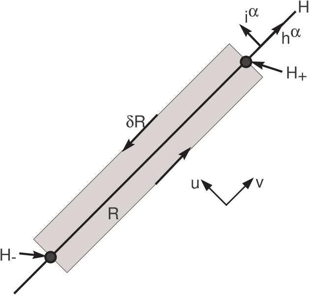
Figure 1: Horizon geometry and the surface $R$. Each point represents a 2-sphere in $(y,z)$.

Since the terms in (10) are total divergences Stokes’ theorem gives

$$-\int_{\partial R}\sqrt{\gamma}n^{\alpha}C_{\alpha\beta}h^{\beta}=8\pi G\int_{\partial R}\sqrt{\gamma}n^{\alpha}T^{(m)}_{\alpha\beta}h^{\beta}$$ (11)

where $n^{\alpha}$ is the normal to the boundary $\partial R$ of $R$ and $\sqrt{\gamma}$ is determinant of the induced metric $\gamma_{\alpha\beta}$ on $\partial R$. I choose $\partial R$ such that $i^{\alpha}$ generates $\partial R$ across $H$. Since $i_{\alpha}$ is proportional to $\partial/\partial v$ and I have the constraints $i^{2},h^{2}\approx 0,i\cdot h=-1$, $i^{\alpha}$ generates translations in the $u$ direction. I will therefore be integrating over $u$ and so can easily evaluate the integral over $\delta(u)$. The right hand side of (11) is simply $8\pi G$ times the total matter flux $\Delta Q$ emanating from the horizon through the surface $\partial R$. Without the constraints this would be zero, corresponding to no anomalous flux for the approximate Killing field $h^{\alpha}$.

I now evaluate the left hand side of (11). $C_{\alpha\beta}h^{\beta}$ is

$$C_{\alpha\beta}h^{\beta}=\delta(u)[-\lambda_{h}h_{\alpha}h^{2}-\lambda_{i}i_{\alpha}$$ (12)

$$+\frac{1}{2}\lambda_{\kappa}(i_{\alpha}h^{\beta}\nabla_{\beta}h^{2}-\nabla_{\alpha}h^{2})-\frac{1}{2}\lambda_{\Theta}P_{\alpha\beta}\dot{h}^{\beta}]$$

$$+h_{\alpha}h^{2}\nabla_{\gamma}(\lambda_{\kappa}\delta(u)i^{\gamma})$$

where I have applied the Liebniz rule to put the $\lambda_{\Theta}$ term in the above form. In the limit as $h^{\alpha}$ is null, the $\lambda_{\Theta}$ term vanishes. The presence of the delta functions implies that there is only a contribution to the integral when $\partial R$ crosses $H$ (the two dimensional surfaces $H_{-},H_{+}$ in Figure 1). Therefore I can safely use the identity $n\cdot i=0$. Contracting with $n^{\alpha}$ and applying $n\cdot i=0$, I have

$$n^{\alpha}C_{\alpha\beta}h^{\beta}=-\delta(u)\lambda_{h}h^{2}(n\cdot h)$$ (13)

$$-\frac{1}{2}\delta(u)\lambda_{\kappa}n^{\alpha}\nabla_{\alpha}h^{2}+(n\cdot h)h^{2}\nabla_{\gamma}(\delta(u)\lambda_{\kappa}i^{\gamma}).$$

I now rewrite the last term in (13) to move the delta function outside the derivative. Using the identity $\delta_{\alpha}^{\beta}=\gamma_{\alpha}^{\beta}-n_{\alpha}n^{\beta}$ the last term can be rewritten as

$$(n\cdot h)h^{2}\nabla_{\gamma}(\delta(u)\lambda_{\kappa}i^{\gamma})$$ (14)

$$=(n\cdot h)h^{2}[D_{\gamma}(\delta(u)\lambda_{\kappa}i^{\gamma})-\delta(u)\lambda_{\kappa}n^{\alpha}n^{\beta}\nabla_{\beta}i_{\alpha}]$$

where $D_{\alpha}=\gamma_{\alpha}^{\beta}\nabla_{\beta}$. The last term in (14) vanishes in the limit $L\rightarrow 0$ as $n^{\alpha}\approx\pm i^{\alpha}/\sqrt{i^{2}}$ and (as chosen previously) $i^{\alpha}$ satisfies the geodesic equation. The plus/minus is present as $n^{\alpha}$ changes orientation from $H_{+}$ (where $n^{\alpha}$ is approximately parallel to $i^{\alpha}$) to $H_{-}$ (where the two vectors are approximately anti-parallel). The $D_{\gamma}$ term in (14) can be integrated over $\partial R$ by parts and becomes

$$-\delta(u)\lambda_{\kappa}i^{\gamma}D_{\gamma}((n\cdot h)h^{2}).$$ (15)

There is no boundary term due to the presence of the delta function. The entire integral in (11) is then proportional to $\delta(u)$. Integrating over the delta function (11) becomes

$$8\pi G\Delta Q=-\int_{H_{+},H_{-}}\sqrt{\gamma}[\lambda_{h}h^{2}(n\cdot h)-\frac{1}{2}\lambda_{\kappa}n^{\alpha}\nabla_{\alpha}h^{2}$$ (16)

$$-\lambda_{\kappa}i^{\gamma}D_{\gamma}((n\cdot h)h^{2})]$$

where the notation $\int_{H_{+},H_{-}}$ signifies that the result is the sum of the integrals over $H_{+}$ and $H_{-}$. Again replacing $n^{\alpha}$ by $\pm{\mathrm{i}}^{\alpha}/\sqrt{i^{2}}$ one sees that the $\lambda_{h}$ term vanishes as $h^{2}\rightarrow 0$. Applying the constraint $\Phi_{\kappa}$, $h^{2}\rightarrow 0$, and (again) the fact that $i^{\alpha}$ satisfies the geodesic equation the last two terms combine and I have

$$8\pi G\Delta Q=\int_{H_{+}}\sqrt{\gamma}\lambda_{\kappa}\frac{\kappa}{\sqrt{i^{2}}}-\int_{H_{-}}\sqrt{\gamma}\lambda_{\kappa}\frac{\kappa}{\sqrt{i^{2}}}$$ (17)

Now note that in this coordinate system $\sqrt{\gamma}$ is equal to $\sqrt{i^{2}}\sqrt{\gamma_{2}}$, where $\gamma_{2}$ is the induced metric on $H_{+},H_{-}$. The factors of $\sqrt{i^{2}}$ cancel and I am finally left with

$$8\pi G\Delta Q=\kappa(\int_{H_{+}}\sqrt{\gamma_{2}}\lambda_{\kappa}-\int_{H_{-}}\sqrt{\gamma_{2}}\lambda_{\kappa}).$$ (18)

If $\lambda_{\kappa}$ varies between $H_{+}$ and $H_{-}$ then there is a non-zero $\Delta Q$ even if the geometry does not change. However, this does not correspond to the case of interest, where the flux is due to the time dependence of the geometry and not the time dependence of the Lagrange multipliers. Therefore $\lambda_{\kappa}$ should be chosen to be a constant. If I choose $\lambda_{\kappa}=1$ then I recover that the generated matter flux satisfies the first law of black hole thermodynamics,

$$8\pi G\Delta Q=\kappa(\int_{H_{+}}\sqrt{\gamma_{2}}-\int_{H_{-}}\sqrt{\gamma_{2}})=\kappa\Delta A$$ (19)

which is the promised result. In summary, I have shown that requiring the presence of a horizon with surface gravity $\kappa$ by imposing constraints in the gravitational action also generates a (necessarily quantum mechanical) matter flux which, at least for Schwarzschild geometry, agrees with the first law of black hole thermodynamics.

IV Discussion

There are some open issues with the above result. The most pressing is obviously the value of $\lambda_{\kappa}$. While the choice $\lambda_{\kappa}=1$ is not an exceptional or fine tuned value, there is no a priori reason why this choice is the correct one. The difficulty in determining $\lambda_{\kappa}$ stems from the fact that I am using the variation of the horizon to determine the generated matter flux without reference to any matter equations of motion. If the (quantum mechanical) matter response was known then it is possible that the value of $\lambda_{\kappa}$ could be fixed by applying the constraint. However, without the matter field equations this method of determining $\lambda_{\kappa}$ is not applicable.

Another open issue is the connection with Carlip’s method for calculating black hole entropy. One would hope that a connection can be made since the underlying approach, applying constraints to force a horizon, is the same. If a connection can be made and in the framework presented here the entropy can be shown to be $A/4$, then the first law is a true thermodynamic equation since in this derivation it relates the outgoing energy flux to the number of microstates of the full quantum theory. There are a few obstacles that still need to be overcome in order to relate the two approaches. Since the horizon surface is a timelike hypersurface here (as it must be to emit Hawking radiation), it is somewhat unclear how to proceed with the Hamiltonian framework. Furthermore, the constraints on the surface gravity do not appear in the formalism of Carlip, so there is no guarantee that the algebra of constraints is identical. If these technical problems can be overcome, then the constraint program might yield not only the number of microstates of a black hole, but also more directly tie Hawking radiation and the laws of black hole thermodynamics to the microscopic theory of quantum gravity.

References

- (1) J. D. Bekenstein, Phys. Rev. D 7, 2333 (1973).
- (2) S. W. Hawking, Nature 248, 30 (1974).
- (3) R. M. Wald, Living Rev. Rel. 4, 6 (2001) [arXiv:gr-qc/9912119].
- (4) S. Carlip, Nucl. Phys. Proc. Suppl. 57, 8 (1997) [arXiv:gr-qc/9702017].
- (5) S. Carlip, Class. Quant. Grav. 22, 1303 (2005) [arXiv:hep-th/0408123].
- (6) S. Carlip, Horizons, Constraints, and Black Hole Entropy, in preparation.
- (7) A. Ashtekar, C. Beetle and S. Fairhurst, Class. Quant. Grav. 16, L1 (1999) [arXiv:gr-qc/9812065].
- (8) A. Ashtekar and B. Krishnan, Living Rev. Rel. 7, 10 (2004) [arXiv:gr-qc/0407042].
- (9) I. Booth, arXiv:gr-qc/0508107.
- (10) S. P. Robinson and F. Wilczek, Phys. Rev. Lett. 95, 011303 (2005) [arXiv:gr-qc/0502074].
- (11) S. M. Christensen and S. A. Fulling, Phys. Rev. D 15, 2088 (1977).
- (12) A. Ashtekar and M. Bojowald, Class. Quant. Grav. 22, 3349 (2005) [arXiv:gr-qc/0504029].