Harmonic Initial-Boundary Evolution in General Relativity

Abstract

Computational techniques which establish the stability of an evolution-boundary algorithm for a model wave equation with shift are incorporated into a well-posed version of the initial-boundary value problem for gravitational theory in harmonic coordinates. The resulting algorithm is implemented as a 3-dimensional numerical code which we demonstrate to provide stable, convergent Cauchy evolution in gauge wave and shifted gauge wave testbeds. Code performance is compared for Dirichlet, Neumann and Sommerfeld boundary conditions and for boundary conditions which explicitly incorporate constraint preservation. The results are used to assess strategies for obtaining physically realistic boundary data by means of Cauchy-characteristic matching.

I Introduction

The ability to compute the details of the gravitational radiation produced by compact astrophysical sources, such as coalescing black holes, is of major importance to the success of gravitational wave astronomy. The simulation of such systems by the numerical evolution of solutions to Einstein’s equations requires a valid treatment of the outer boundary. This involves the mathematical issue of proper boundary conditions which ensure a well-posed initial-boundary value problem (IBVP), the computational issues of the consistency, accuracy and stability of the finite difference approximation, and the physical issue of prescribing boundary data which is free of spurious incoming radiation. The physical issue can be solved by locating the outer boundary at future null infinity ${\cal I}^{+}$ in a conformally compactified spacetime penrose . Since no light rays can enter the spacetime through ${\cal I}^{+}$, no boundary data are needed to evolve the interior spacetime. In addition, the waveform and polarization of the outgoing radiation can be unambiguously calculated at ${\cal I}^{+}$ in terms of the Bondi news function. This global approach has been applied to single black hole spacetimes using Cauchy evolution on hyperboloidal time slices (see Hhprbloid ; joerg for reviews) and using characteristic evolution on null hypersurfaces(see winrev for a review). However, most current computational work on the binary black hole problem involves Cauchy evolution in a domain whose outer boundary is a finite timelike worldtube. This approach could be justified physically if the boundary data were supplied by matching to an exterior solution extending to ${\cal I}^{+}$. The present work is part of a Cauchy-characteristic matching (CCM) project vishu ; harl to achieve this by matching the interior Cauchy evolution to an exterior characteristic evolution. The success of CCM depends upon the proper mathematical and computational treatment of the Cauchy IBVP. A key issue, on which we focus in this paper, is the accurate preservation of the constraints in the treatment of the Cauchy boundary. The results have important bearing on the matching problem.

Early computational work in general relativity focused on the initial value problem in which data on a spacelike hypersurface ${\cal S}$ determines the evolution in its domain of dependence. However, in the simulation of an isolated system, such as a neutron star or black hole, ${\cal S}$ typically has an outer timelike boundary ${\cal B}$, coincident with the boundary of the computational grid. The initial-boundary value problem addresses the extension of the evolution into the domain of dependence of ${\cal S}\cup{\cal B}$. The IBVP for Einstein’s equations is still not well understood due to complications arising from the constraint equations. See friedrend for a review of the mathematical aspects. Well-posedness of the mathematical problem, which guarantees the existence and uniqueness of a solution with continuous dependence on the Cauchy and boundary data, is a necessary condition for computational success. A well-posed IBVP for a linearization of the Einstein equations was first presented by Stewart stewartbc , and the first well-posed version for the full nonlinear theory was established by Friedrich and Nagy Friedrich98 . These works have influenced numerous investigations of the implementation of boundary conditions in numerical relativity bishbc ; szilschbc ; harl ; callehtigbc ; calpulreulbc ; fritgombc ; fritgombc3 ; bab ; fritgombc4 ; sartig ; gunmgarcbc ; caltechbc ; bonabc ; multiblock ; calabgund ; linsch . However, the combined mathematical and computational aspects of the IBVP still present a major impasse in carrying out the long term simulations necessary to compute useful waveforms from the inspiral and merger of black holes.

The IBVP for general relativity takes on one of its simplest forms in a harmonic gauge, in which the well-posedness of the Cauchy problem was first established Choquet . In previous work, we formulated a well-posed constraint preserving version of the harmonic IBVP and implemented it as a numerical code harl , the Abigel code. The IBVP was demonstrated to be well-posed for homogeneous boundary data (or for small boundary data in the sense of linearization off homogeneous data) and the code was shown to be stable and convergent. Nevertheless, numerical evolution was limited by the excitation of exponential instabilities of an analytic origin. Insight into the nature of these unstable modes and mathematical and computational techniques for dealing with them have been developed in a study of the evolution problem in the absence of boundaries. These studies were carried out on toroidal spatial manifolds, equivalent to the imposition of periodic boundary conditions. In this paper, we apply the techniques which were successful in the periodic case to the general harmonic IBVP. Although our applications here are limited to test problems, we expect the techniques will be of benefit in furthering recent progress in the simulation of black holes by harmonic evolution pret1 ; pret2 ; linsch .

Our previous work on the IBVP harl was based upon a reduced form of the harmonic system due to Fock Fock . We present our results here in the more standard form wald ; friedrend used in most analytic work. We have described and tested a finite difference evolution code based upon this standard harmonic formulation in babev . In Sec. II, we summarize the main analytic and computational features of this evolution code. The formalism includes harmonic gauge forcing terms and constraint adjustments. In principle, gauge forcing terms Friedrich allow the simulation of any nonsingular spacetime region. Gauge forcing not only allow the flexibility to “steer” around pathologies that might otherwise arise in standard harmonic coordinates but it also allows universal adaptability to carry out standardized tests for code performance, such as the AppleswithApples (AwA) tests mex1 . The formalism also includes constraint adjustments which modify the nonlinear terms in the standard harmonic equations by mixing in the harmonic constraints. Such constraint adjustments have proved to be important in harmonic evolution in suppressing instabilities in a shifted version of the AwA gauge wave test babev and in simulating black holes pret1 ; pret2 .

Constraint adjustments, when combined with a flux conservative form of the equations, can lead to conserved quantities which suppress exponentially growing error modes. As a dramatic example, the AwA gauge wave tests for the Abigel harmonic code show an increase in error of more than 12 orders of magnitude, after 100 grid crossing times, if flux conservation is not employed bab . The error arises from exponentially growing solutions to the reduced equations which have long wavelength and satisfy the constraints, so that it is unaffected by either numerical dissipation or constraint adjustment. The underlying conservation laws only apply to the prinicple part of the system. The are effective when the nonlinear terms corresponding to the unstable modes are small, or can be adjusted to be small by mixing in the constraints. This is the case with the AwA gauge wave. However, as we discuss in Sec. II, a shifted version of the gauge wave test excites a different type of exponential instability which does not satisfy the constraints and whose suppression requires constraint adjustment in addition to flux conservation. This raises the caveat that the identification of the nonlinear instabilities in the system is critical to the effectiveness of constraint adjustment and conservative techniques.

In Sec’s III and IV, we describe how our earlier proof harl of the well-posedness of the harmonic IBVP for Einstein’s equations extends to the generalized formulation considered here. Constraint preservation imposes requirements coupling the intrinsic metric and extrinsic curvature of the boundary, analogous to the momentum constraint on Cauchy data. However, the boundary data has fewer degrees of freedom than the corresponding Cauchy data, as for a scalar field where either the field or its normal derivative, but not both, can be specified on the boundary. This couples the evolution to the specification of constraint-preserving boundary data in a way that the standard theorems used to establish well-posedness only apply to boundary data linearized off homogeneous boundary data. In the case of large boundary data, one is only assured that the solution, if it exists, does satisfy the constraints.

In Sec. V, we present the techniques used to implement the formalism as a finite difference evolution-boundary algorithm. Since the preliminary testing of the Abigel code, considerable improvement has been made in the numerical techniques. The long term performance of the evolution algorithm in the AwA gauge wave test with periodic boundaries has been improved by use of semi-discrete conservation laws bab . The study of a model nonlinear scalar wave excis shows how these semi-discrete conservation laws can be used to formulate stable algorithms for more general boundary conditions.

In Sec. VI, we demonstrate the stability and second order convergence of the code for periodic, Neumann, Dirichlet and Sommerfeld boundary conditions. These tests are performed using gauge wave and shifted gauge wave metrics for which the exact solutions provide the correct boundary data. In principle, the knowledge of the exact boundary data avoids the need for constraint-preserving boundary conditions. However, numerical noise can generate constraint violating error. This is investigated by comparing these constraint free boundary algorithms against the constraint-preserving algorithm discussed in Sec’s III and IV. In order to eliminate the complication of sharp boundary points, the tests are carried out by opening up the 3-torus (periodic boundary) into a 2-torus times a line, with two smooth 2-toroidal boundaries.

Just as the “3+1” decomposition $x^{\mu}=(t,x^{i})$ is useful in describing the geometry of a spacelike Cauchy hypersurface ${\cal S}$ at $t=0$, the decomposition $x^{\mu}=(x^{a},x)$, with $x^{a}=(t,y,z)$ is useful in describing the geometry of a timelike boundary ${\cal B}$ at $x=0$. We distinguish between these decompositions by using indices $i,j,k,...$ near the middle of the alphabet or indices $a,b,c,...$ at the beginning of the alphabet. In order to avoid excessive notation we indicate the corresponding intrinsic 3-metrics by $h_{ij}$ and $h_{ab}$, with inverses $h^{ij}$ and $h^{ab}$. Where this might cause confusion, we introduce subscripts, e.g. $h_{\cal S}=det(h_{ij})$ and $h_{\cal B}=det(h_{ab})$. Curvature conventions follow wald . This introduces some sign changes from the treatment in harl which was based upon the conventions in Fock . We use the shorthand notation $\partial_{\alpha}f=f_{,\alpha}$ where confusion does not arise.

II The generalized harmonic Cauchy problem

We summarize here the treatment of the generalized harmonic Cauchy problem on which the evolution code described in babev is based. Generalized harmonic coordinates $x^{\alpha}=(t,x^{i})=(t,x,y,z)$ are functionally independent solutions of the curved space scalar wave equation,

$$\Box x^{\mu}=\frac{1}{\sqrt{-g}}\partial_{\alpha}(\sqrt{-g}g^{\alpha\beta}\partial_{\beta}x^{\mu})=-\hat{\Gamma}^{\mu}.$$ (1)

where the gauge source terms $\hat{\Gamma}^{\mu}(x^{\alpha},g_{\alpha\beta})$ can have functional dependence on the coordinates and the metric Friedrich . In terms of the connection $\Gamma^{\mu}_{\alpha\beta}$, these harmonic conditions take the form

$${\cal C}^{\mu}:=\Gamma^{\mu}-\hat{\Gamma}^{\mu}=0.$$ (2)

where

$$\Gamma^{\mu}=g^{\alpha\beta}\Gamma^{\mu}_{\alpha\beta}=-\frac{1}{\sqrt{-g}}\partial_{\alpha}\gamma^{\alpha\mu}$$ (3)

and $\gamma^{\mu\nu}=\sqrt{-g}g^{\mu\nu}$. The standard harmonic reduction of the Einstein tensor (see e.g. wald ; Friedrich ) is

$$E^{\mu\nu}:=G^{\mu\nu}-\nabla^{(\mu}\Gamma^{\nu)}+\frac{1}{2}g^{\mu\nu}\nabla_{\alpha}\Gamma^{\alpha},$$ (4)

where $\Gamma^{\nu}$ is treated formally as a vector in constructing the “covariant” derivatives $\nabla^{\mu}\Gamma^{\nu}$. Explicitly in terms of the metric,

$$2\sqrt{-g}E^{\mu\nu} = \partial_{\alpha}(g^{\alpha\beta}\partial_{\beta}\gamma^{\mu\nu})-2\sqrt{-g}g^{\alpha\rho}g^{\beta\sigma}\Gamma^{\mu}_{\alpha\beta}\Gamma^{\nu}_{\rho\sigma}-\sqrt{-g}(\partial_{\alpha}g^{\alpha\beta})\partial_{\beta}g^{\mu\nu}+\frac{1}{\sqrt{-g}}g^{\alpha\beta}(\partial_{\beta}g)\partial_{\alpha}g^{\mu\nu}$$ (5)

$$+ \frac{1}{2}g^{\mu\nu}\bigg{(}\frac{1}{2g\sqrt{-g}}g^{\alpha\beta}(\partial_{\alpha}g)\partial_{\beta}g+\sqrt{-g}\Gamma^{\rho}_{\alpha\beta}\partial_{\rho}g^{\alpha\beta}+\frac{1}{\sqrt{-g}}(\partial_{\beta}g)\partial_{\alpha}g^{\alpha\beta}\bigg{)}.$$

Thus the standard harmonic evolution equations are quasilinear wave equations $E^{\mu\nu}=0$ for the components of the densitized metric $\gamma^{\mu\nu}$. The principle part of (5) has been expressed in the flux conservative form

$$\partial_{\alpha}(g^{\alpha\beta}\partial_{\beta}\gamma^{\mu\nu}).$$ (6)

In the particular case of the AwA gauge wave, the vanishing of the nonlinear source terms then leads to the exact conservation laws for the quantitities

$$Q^{\mu\nu}=-\int_{V}g^{t\alpha}\partial_{\alpha}\gamma^{\mu\nu}dV.$$ (7)

The semi-discrete version of these conservation laws suppresses instabilities in the AwA gauge wave test. (See babev for details.)

This standard treatment of the Cauchy problem in harmonic coordinates generalizes in a straightforward way to include harmonic gauge source terms and constraint adjustments of the form

$$A^{\mu\nu}={\cal C}^{\rho}A^{\mu\nu}_{\rho}(x^{\alpha},g^{\alpha\beta},\partial_{\gamma}g^{\alpha\beta}).$$ (8)

The reduced equations then become

$$\tilde{E}^{\mu\nu}: = G^{\mu\nu}-\nabla^{(\mu}{\cal C}^{\nu)}+\frac{1}{2}g^{\mu\nu}\nabla_{\alpha}{\cal C}^{\alpha}+A^{\mu\nu}$$ (9)

$$= E^{\mu\nu}+\nabla^{(\mu}\hat{\Gamma}^{\nu)}-\frac{1}{2}g^{\mu\nu}\nabla_{\alpha}\hat{\Gamma}^{\alpha}+A^{\mu\nu}=0.$$

Since the gauge source terms and constraint adjustments do not enter the principle part, (9) also constitute a system of quasilinear wave equations with a well-posed Cauchy problem.

The solutions of the generalized harmonic evolution system (9) are solutions of the Einstein equations provided the harmonic constraints

$${\cal C}^{\mu}:=\Gamma^{\mu}-\hat{\Gamma}^{\mu}=0$$ (10)

are satisfied. The Bianchi identities, applied to (9), imply that these constraints obey the homogeneous wave equations

$$\nabla^{\alpha}\nabla_{\alpha}{\cal C}^{\mu}+R^{\mu}_{\nu}{\cal C}^{\nu}-2\nabla_{\nu}({\cal C}^{\rho}A^{\mu\nu}_{\rho})=0,$$ (11)

where via (9) the Ricci tensor reduces to

$$R^{\mu\nu}=\nabla^{(\mu}{\cal C}^{\nu)}-{\cal C}^{\rho}(A^{\mu\nu}_{\rho}-\frac{1}{2}g^{\mu\nu}g_{\alpha\beta}A^{\alpha\beta}_{\rho}).$$ (12)

The well-posedness of the Cauchy problem for (11) implies the unique solution ${\cal C}^{\mu}=0$ in the domain of dependence of the initial Cauchy hypersurface ${\cal S}$ provided the Cauchy data $\gamma^{\mu\nu}|_{\cal S}$ and $\partial_{t}\gamma^{\mu\nu}|_{\cal S}$ satisfy ${\cal C}^{\mu}|_{\cal S}=\partial_{t}{\cal C}^{\mu}|_{\cal S}=0$ via (9). It is straightforward to verify that Cauchy data on ${\cal S}$ which satisfy the Hamiltonian and momentum constraints $G^{t}_{\mu}=0$ and the initial condition ${\cal C}^{\mu}=0$ also satisfy $\partial_{t}{\cal C}^{\mu}=0$ on ${\cal S}$ by virtue of the reduced harmonic equations (9). In addition to the standard Cauchy data for the $3+1$ decomposition, i.e. the intrinsic metric and extrinsic curvature of ${\cal S}$ subject to the Hamiltonian and momentum constraints, the only other free data are the initial choices of $\gamma^{t\alpha}$, equivalent to the initial choices of lapse and shift.

The standard harmonic reduction (4) differs from Fock’s Fock harmonic formulation adopted in harl by the adjustment

$$A^{\mu\nu}=\frac{1}{2g}{\cal C}^{(\mu}g^{\nu)\alpha}\partial_{\alpha}g-\frac{1}{4g}g^{\mu\nu}{\cal C}^{\alpha}\partial_{\alpha}g.$$ (13)

In the tests of the boundary algorithms in Sec. VI, we have examined the effects of the adjustments

$$A^{\mu\nu} = -\frac{a_{1}}{\sqrt{-g}}{\cal C}^{\alpha}\partial_{\alpha}(\sqrt{-g}g^{\mu\nu})$$ (14)

$$A^{\mu\nu} = \frac{a_{2}{\cal C}^{\alpha}\nabla_{\alpha}t}{e_{\rho\sigma}{\cal C}^{\rho}{\cal C}^{\sigma}}{\cal C}^{\mu}{\cal C}^{\nu}$$ (15)

$$A^{\mu\nu} = -\frac{a_{3}}{\sqrt{-g^{tt}}}{\cal C}^{(\mu}\nabla^{\nu)}t,$$ (16)

where the $a_{i}>0$ are positive adjustable parameters and

$$e_{\rho\sigma}=g_{\rho\sigma}-\frac{2}{g^{tt}}(\nabla_{\rho}t)\nabla_{\sigma}t$$ (17)

is the natural metric of signature $(++++)$ associated with the Cauchy slicing. The adjustments (14) and (15) were effective in suppressing instabilities in the shifted gauge wave tests without boundaries babev . (For numerical purposes, the limit as $C^{\mu}\rightarrow 0$ in (15) can be regularized by a small positive addition to the denominator.) The adjustment (16) leads to constraint damping constrdamp in the linear regime and has been used effectively in black hole simulations pret2 but was not effective in the nonlinear shifted gauge wave test.

III Well-posedness of the homogeneous initial-boundary value problem

In prior work harl we showed how the well-posedness of the Cauchy problem for the standard harmonic formulation of Einstein’s equations extends to the IBVP with homogeneous boundary data. Here we show how the well-posedness of the IBVP extends to include harmonic gauge forcing terms and constraint adjustments. Our approach is based upon a theorem of Secchi secchi2 for first order, quasilinear, symmetric hyperbolic systems. For that purpose, we recast the reduced system (9) in first order form in terms of the 50-dimensional column vector ${\bf u}={}^{T}(\gamma^{\alpha\beta},{\cal T}^{\alpha\beta},{\cal X}^{\alpha\beta},{\cal Y}^{\alpha\beta},{\cal Z}^{\alpha\beta})$ (the transpose of the row vector ${}^{T}{\bf u}$) where ${\cal T}^{\alpha\beta}=\partial_{t}\gamma^{\alpha\beta}$, ${\cal X}^{\alpha\beta}=\partial_{x}\gamma^{\alpha\beta}$, ${\cal Y}^{\alpha\beta}=\partial_{y}\gamma^{\alpha\beta}$ and ${\cal Z}^{\alpha\beta}=\partial_{z}\gamma^{\alpha\beta}$. Equation (9) then has the quasilinear, symmetric hyperbolic form

$${\bf A}^{t}\partial_{t}{\bf u}+{\bf A}^{i}\partial_{i}{\bf u}={\bf S}$$ (18)

where ${\bf A}^{t}$ and ${\bf A}^{i}$ are 50-dimensional symmetric matrices, with ${\bf A}^{t}$ positive definite, and ${\bf S}$ is a 50-dimensional column vector, all depending only on the components of ${\bf u}$. For explicit values of the matrices ${\bf A}^{t}$ and ${\bf A}^{i}$ see App. A.

Consider the IBVP for the reduced Einstein equations for the generalized harmonic system in the domain $t\geq 0$, $x\leq 0$, with timelike boundary ${\cal B}$ at $x=0$. (Any boundary can be constructed by patching together such pieces.) Secchi’s theorem establishes well-posedness of the IBVP for (18) under weak regularity assumptions by imposing a homogeneous boundary condition based upon the energy norm

$$E=\frac{1}{2}\int^{T}{\bf uu}dxdydz.$$ (19)

and the associated local energy flux across the boundary

$${\cal F}^{x}=\frac{1}{2}{}^{T}{\bf u}{\bf A}^{x}{\bf u}.$$ (20)

The chief requirement for a well-posed IBVP is that the boundary condition be maximally dissipative, which allows energy estimates to be established. Explicitly, the requirements at $x=0$ are

• that the kernel of the boundary matrix ${\bf A}^{x}$ must have constant dimension,

• that the boundary condition must take the matrix form ${\bf Mu}=0$ for homogeneous boundary data, where ${\bf M}$ is independent of ${\bf u}$ and has maximal dimension consistent with the system of equations

• and, for all ${\bf u}$ satisfying the boundary condition, that the boundary flux satisfy the inequality

  $${\cal F}^{x}\geq 0.$$ (21)

In addition, compatibility conditions between the Cauchy and boundary data at $t=x=0$ must be satisfied.

As a result of reducing the harmonic Einstein equations to first order symmetric hyperbolic form, there are variables associated with characteristics which propagate tangential to the boundary. Secchi’s theorem applies to this case of a characteristic boundary in which the matrix ${\bf A}^{x}$ is degenerate. The matrix ${\bf M}$ can depend explicitly on the coordinates but not upon the evolution variables ${\bf u}$. The maximal dimension of ${\bf M}$ is directly related to how many variables propagate toward the boundary from the exterior. Variables in the kernel of ${\bf A}^{x}$, which propagate tangential to the boundary, and variables which propagate from the interior toward the boundary require no boundary condition. The possible choices of matrix ${\bf M}$ correspond to the nature of the boundary condition, e.g. Dirichlet, Sommerfeld or Neumann.

We now formulate such maximally dissipative boundary conditions for the reduced harmonic system. The principal part consists of the term $g^{\alpha\beta}\partial_{\alpha}\partial_{\beta}\gamma^{\mu\nu}$, which represents a wave operator acting on the 10 components $\gamma^{\mu\nu}$. As a result, the energy flux ${\cal F}^{x}$ equals the sum of 10 individual fluxes, each of which corresponds to the standard energy flux constructed from the stress-energy tensor obtained by treating each component of $\gamma^{\mu\nu}$ as a massless scalar field. Thus we can pattern our analysis of the IBVP on the scalar wave equation

$$g^{\mu\nu}\partial_{\mu}\partial_{\nu}\Phi=0,$$ (22)

which is discussed in App. A. When $\Phi$ is regarded as an independent scalar field rather than as a component of $\gamma^{\mu\nu}$, the linearity of (22) implies well-posedness for any of the dissipative boundary conditions discussed in App. A, e.g. generalized Dirichlet, Neumann or Sommerfeld boundary conditions.

We can decompose the boundary conditions for the full gravitational problem into the five 10-dimensional subspaces corresponding to $\gamma^{\alpha\beta}$, ${\cal T}^{\alpha\beta}$, ${\cal X}^{\alpha\beta}$, ${\cal Y}^{\alpha\beta}$ and ${\cal Z}^{\alpha\beta}$. The subspace corresponding to $\gamma^{\alpha\beta}$ lies in the kernel of ${\bf A}^{x}$ and requires no boundary condition, i.e the boundary values of $\gamma^{\alpha\beta}$ are determined by boundary values of the other variables. The remaining four subspaces require boundary conditions analogous to the scalar field case. The extra complications in the quasi-linear gravitational case are to check that the constraints are satisfied and that the linear subspace ${\bf Mu}=0$ is specified independent of ${\bf u}$.

For that purpose, we adapt the harmonic coordinate system to the boundary. In doing so, we use the $3+1$ decomposition natural to the boundary at $x=0$ and write $x^{\alpha}=(x^{a},x)$, where $x^{a}=(t,y,z)$. Our approach is motivated by the observation that the initial value problem is well-posed so that reflection symmetric Cauchy data in the neighborhood $-\epsilon<x<\epsilon$ produces a solution with even parity. From the point of view of the IBVP in the region $x\leq 0$, this solution induces homogeneous boundary data of either the Neumann or Dirichlet type on each metric component, depending upon how that component transforms under reflection.

III.1 The boundary gauge

Local to the boundary ${\cal B}$, it is always possible to choose Gaussian normal coordinates $(\tilde{x}^{a},\tilde{x})$ so that the boundary is given by $\tilde{x}=0$ and $g^{\tilde{x}\tilde{a}}=0$ vanishes at the boundary. Now consider a coordinate transformation to generalized harmonic coordinates $(x^{a},x)$ satisfying $\Box x^{\alpha}=-\hat{\Gamma}^{\alpha}$. Since $g^{\tilde{x}\tilde{a}}=0$, the analysis in App. A shows that it is possible to solve this wave equation with either the homogeneous Dirichlet condition $\Phi=0$ or the homogeneous Neumann condition $\partial_{x}\Phi=0$. For the harmonic coordinate $x$, we choose the Dirichlet condition $x|_{\cal B}=0$, so that ${\cal B}$ remains located at $x=0$; and for the remaining harmonic coordinates, we choose the Neumann condition $\partial_{\tilde{x}}x^{a}|_{\cal B}=0$.

These choices exhaust the boundary freedom in constructing generalized harmonic coordinates. After transforming to these harmonic coordinates, the metric satisfies

$$\gamma^{xa}|_{\cal B}=0.$$ (23)

We enforce this as the dissipative Dirichlet boundary condition

$${\cal T}^{xa}|_{\cal B}=0,$$ (24)

subject to initial data satisfying (23).

In this boundary gauge, the results of App. A imply that the homogeneous Neumann boundary conditions

$${\cal X}^{xx}|_{\cal B}={\cal X}^{ab}|_{\cal B}=0,$$ (25)

are also dissipative, as well as the Sommerfeld-like conditions

$$({\cal T}^{xx}+{\cal X}^{xx})|_{\cal B}=({\cal T}^{ab}+{\cal X}^{ab})|_{\cal B}=0.$$ (26)

Given that the boundary gauge condition (23) is satisfied, any combination of Dirichlet, Sommerfeld-like and Neumann boundary conditions on the remaining components leads to a well-posed IBVP for the reduced generalized harmonic system (9). Note, however, that a Sommerfeld condition corresponding to the null direction defined by normal to the boundary,

$$({\cal T}^{xx}+\frac{\sqrt{-g_{tt}}}{\sqrt{g_{xx}}}{\cal X}^{xx})|_{\cal B}=({\cal T}^{ab}+\frac{\sqrt{-g_{tt}}}{\sqrt{g_{xx}}}{\cal X}^{ab})|_{\cal B}=0,$$ (27)

does not satisfy the technical condition in Secchi’s theorem that $M$ be independent of $u$.

III.2 The homogeneous constraint-preserving boundary condition

The constraints ${\cal C}^{\mu}=\Gamma^{\mu}-\hat{\Gamma}^{\mu}$ satisfy the homogeneous wave equation (11), which can be reduced to symmetric hyperbolic form. Consequently, we can force them to vanish by choosing boundary conditions for the reduced system which force ${\cal C}^{\mu}$ to satisfy a maximally dissipative homogeneous boundary condition. In doing so, we shall require that the normal components of the gauge source function and constraint adjustment vanish on the boundary, i.e.

$$\hat{\Gamma}^{x}|_{\cal B} = 0$$

$$A^{ax}|_{\cal B} = 0.$$ (28)

These requirements are a consequence of the reflection properties of the boundary in the homogeneous case.

We proceed by imposing boundary conditions on the evolution system consisting of the Dirichlet boundary-gauge conditions (23) and the Neumann conditions (25), which imply

$$\gamma^{ax}|_{\cal B}=\partial_{x}\gamma^{xx}|_{\cal B}=\partial_{x}\gamma^{ab}|_{\cal B}=\partial_{x}g|_{\cal B}=0.$$ (29)

As we shall show, (23) and (29) further imply that the constraints obey the maximally dissipative homogeneous boundary conditions

$$\partial_{t}{\cal C}^{x}|_{\cal B} = 0$$ (30)

$$\partial_{x}{\cal C}^{a}|_{\cal B} = 0.$$ (31)

Note that (30) and (31) are satisfied by any geometry which has local reflection symmetry with respect to the boundary if the gauge source functions $\hat{\Gamma}^{\alpha}$ share this symmetry (as a vector). In order to verify (30), we note that

$$\partial_{t}{\cal C}^{x}=-\partial_{t}\bigg{(}\frac{1}{\sqrt{-g}}(\partial_{x}\gamma^{xx}+\partial_{a}\gamma^{xa})+\hat{\Gamma}^{x}\bigg{)}$$ (32)

vanishes on the boundary as a consequence of (28) and (29).

Similarly, in order to verify (31), we note that

$$\partial_{x}{\cal C}^{a}=-\partial_{x}\bigg{(}\frac{1}{\sqrt{-g}}(\partial_{x}\gamma^{ax}+\partial_{b}\gamma^{ab})+\hat{\Gamma}^{a}\bigg{)}$$ (33)

reduces on the boundary to

$$\partial_{x}{\cal C}^{a}|_{\cal B}=-\bigg{(}\frac{1}{\sqrt{-g}}\partial_{x}^{2}\gamma^{ax}+\partial_{x}\hat{\Gamma}^{a}\bigg{)}|_{\cal B}.$$ (34)

Now we use the $\tilde{E}^{ax}=0$ component of the evolution equation to eliminate $\partial_{x}^{2}\gamma^{ax}$. Substitution of the assumed boundary conditions into (5) gives

$$E^{ax}|_{\cal B}=\frac{g^{xx}}{2\sqrt{-g}}\partial_{x}^{2}\gamma^{ax}|_{\cal B}.$$ (35)

Then (9) gives

$$0=\tilde{E}^{ax}|_{\cal B}=\frac{g^{xx}}{2}\bigg{(}\frac{1}{\sqrt{-g}}\partial_{x}^{2}\gamma^{ax}+\partial_{x}\hat{\Gamma}^{a}\bigg{)}|_{\cal B}+A^{ax}|_{\cal B},$$ (36)

which, together with (28) and (34), establishes (31).

In summary, the maximally dissipative boundary conditions (23) and (25) for the evolution variables ${\bf u}$ imply the maximally dissipative homogeneous boundary conditions (30) and (31) for the constraints. This establishes the boundary data necessary to show that the harmonic constraints ${\cal C}^{\mu}=0$ propagate if the initial Cauchy data satisfy the Hamiltonian and momentum constraints.

The remaining ingredient necessary for a well-posed initial-boundary problem is the consistency between the initial Cauchy data and the boundary data. The order of consistency determines the order of differentiability of the solution. The simplest case to analyze is prescription of initial data with locally smooth reflection symmetry at the boundary, e.g Cauchy data $\gamma^{ab}(0,x,y,z)$ for $x\leq 0$ whose extension to $x\geq 0$ by reflection would yield a $C^{\infty}$ function in the neighborhood of $x=0$. Such data are automatically consistent with the homogeneous boundary conditions given above.

We could also have established the boundary conditions (31) for the constraints indirectly, but with a more geometric argument, by noting that the boundary conditions (29) for the metric imply that the extrinsic curvature of the boundary vanishes, which in turn implies that the $G^{ax}$ components of the Einstein tensor vanish at the boundary (see App. B). Thus, along with the evolution equation $\tilde{E}^{ax}=0$, (9) implies

$$-\nabla^{(a}{\cal C}^{x)}+\frac{1}{2}g^{ax}\nabla_{\alpha}{\cal C}^{\alpha}+A^{ax}=0.$$ (37)

This, combined with (28) - (30), now gives (31). We take this geometrical approach in the next section in analyzing the difficulties underlying extending these results to include inhomogeneous boundary data.

IV Inhomogeneous boundary data

In the preceding section we showed that the generalized harmonic evolution system $\tilde{E}^{\mu\nu}=0$ gives rise to a well-posed constraint-preserving IBVP with a variety of maximally dissipative homogeneous boundary conditions. The well-posedness of this IBVP for the reduced system extends by standard arguments to include inhomogeneous data. However, only for special choices of the boundary data is the solution guaranteed to satisfy the constraints. For example, in the simulation of a known analytic solution to Einstein’s equations, when the initial data and boundary data are supplied by their analytic values, the well-posedness of the IBVP guarantees a unique and therefore constraint-preserving solution. This example is important in code development for carrying out tests of the type reported in Sec. VI. Similarly, when an exterior solution of the Einstein equations is supplied in another patch overlapping the boundary, the induced boundary data are constraint-preserving. This possibility arises in Cauchy-characteristic matching. Except for such examples, the specification of free boundary data for the reduced system does not in general lead to a solution of the Einstein equations.

We now formulate conditions on the inhomogeneous boundary data which are sufficient to guarantee that the IBVP for the generalized harmonic system leads to a solution that satisfies the constraints. However, because the matrix ${\bf M}$ used in formulating these constraint-preserving boundary conditions depends on the evolution variables ${\bf u}$, the well-posedness of the resulting IBVP follows from Secchi’s theorems only for “small” boundary data, in the sense of linearization about a solution with homogeneous data. Well-posedness for “large” boundary data remains an open question.

As in the homogeneous case, we consider the IBVP in the domain $t\geq 0$, $x\leq 0$. We first generalize the boundary gauge condition (23). Given harmonic coordinates $x^{\nu}$ such that $\gamma^{xa}|_{\cal B}=0$ at $x=0$, consider the effect of a harmonic coordinate transformation $\tilde{x}^{\mu}(x^{\nu})$ satisfying $\Box\tilde{x}^{\mu}=-\hat{\Gamma}^{\mu}$. For simplicity, we assign initial Cauchy data $\tilde{x}^{\mu}=x^{\mu}$ and $\partial_{t}\tilde{x}^{\mu}=\partial_{t}x^{\mu}$ at $t=0$ and require that the boundary remain located at $\tilde{x}=0$. By uniqueness of solutions to the IBVP for the wave equation, this Dirichlet boundary data for $\tilde{x}$ determines that $\tilde{x}=x$ everywhere in the evolution domain so that $\tilde{x}^{\mu}=(\tilde{x}^{a},x)$. The coordinates $\tilde{x}^{a}$ are uniquely determined by the Neumann boundary data $q^{a}=\partial_{x}\tilde{x}^{a}|_{\cal B}$, which can be assigned freely. Under this transformation, $\gamma^{\tilde{x}\tilde{a}}=q^{a}\gamma^{\tilde{x}\tilde{x}}$ at the boundary, so that $\gamma^{\tilde{x}\tilde{a}}/\gamma^{\tilde{x}\tilde{x}}$ can be freely specified as boundary data $q^{a}(x^{b})$. (Consistency conditions would require that $q^{a}=0$ at $t=x=0$. However, the initial value of $q^{a}$ can be freed up by a deformation of the initial Cauchy hypersurface in the neighborhood of the boundary.) In the remainder of this section, we assume that this transformation has been made and that the $\tilde{x}^{\mu}(x^{\nu})$ coordinates have been relabeled $x^{\mu}$. Thus, in this coordinate system,

$$q^{a}(x^{b})=\frac{\gamma^{xa}}{\gamma^{xx}}|_{\cal B}$$ (38)

is free boundary data representing the choice of boundary gauge at $x=0$.

Although it might seem that such a gauge transformation would not disturb the well-posed nature of the IBVP problem for the reduced system, already (38) introduces the complication that Dirichlet boundary data for $\gamma^{xa}$ cannot be determined from $q^{a}$ unless $\gamma^{xx}$ is known on the boundary. But the boundary condition (29) for $\gamma^{xx}$ is of Neumann type so that $\gamma^{xx}|_{\cal B}$ can only be determined after carrying out the evolution and, in particular, depends on the initial Cauchy data. This is the first source of the ${\bf u}$-dependence of the matrix ${\bf M}$ expressing the boundary condition. It would seem that this problem might be avoided by using $\gamma^{xa}/\gamma^{xx}$ as an evolution variable but, as will become apparent, more complicated (differential) problems of this type arise in introducing inhomogeneous constraint preserving boundary data for the remaining variables.

The complete set of free boundary data for the generalized harmonic system, which in the inhomogeneous case replaces the maximally dissipative homogeneous boundary conditions (23) and (29), consist of

$${\bf q}=(q^{a},q^{xx},q^{ab})=(q^{a},q^{\mu}\partial_{\mu}\gamma^{xx},q^{\mu}\partial_{\mu}\gamma^{ab})|_{\cal B},$$ (39)

where, in accord with (38),

$$q^{\mu}=(q^{a},1)=\frac{1}{g^{xx}}\nabla^{\mu}x=\frac{1}{\sqrt{g^{xx}}}n^{\mu},$$ (40)

with $n^{\mu}$ the unit outward normal to the boundary.

Note that a dissipative Neumann condition must be formulated in terms of the normal derivative $q^{\mu}\partial_{\mu}$ and not the $\partial_{x}$ derivative used in the previous section where $q^{a}=0$. For this purpose, it is useful to introduce the projection tensor into the tangent space of the boundary,

$$h_{\mu}^{\nu}=\delta_{\mu}^{\nu}-n_{\mu}n^{\nu}.$$ (41)

The extrinsic curvature tensor of the boundary is given by

$$K^{\mu\nu}=h^{\mu}_{\alpha}h^{\nu}_{\beta}\nabla^{\alpha}n^{\beta}.$$ (42)

Its explicit expression in terms of the harmonic variables used here is given in App. B.

The inhomogeneous boundary data ${\bf q}$ must be constrained if the Einstein equations are to be satisfied. The subsidiary system of equations which governs the constraints requires a slightly more complicated treatment than in the previous section. For its analysis, we represent the constraints by ${\bf C}=(C^{x},C_{a}=g_{a\mu}C^{\mu})$. Since $C^{\mu}=(C^{x}n_{x}-C_{a}n^{a})n^{\mu}+C_{a}g^{a\mu}$, it is clear that ${\bf C}=0$ is equivalent to $C^{\mu}=0$. It is straightforward to show, beginning with (11), that ${\bf C}$ satisfies a wave equation of the homogeneous form

$$g^{\mu\nu}\partial_{\mu}\partial_{\nu}{\bf C}+{\bf P}^{\mu}\partial_{\mu}{\bf C}+{\bf Q}{\bf C}=0,$$ (43)

where the elements of the square matrices ${\bf P}^{\mu}$ and ${\bf Q}$ depend algebraically on the evolution variables ${\bf u}$. This system can be converted to symmetric hyperbolic first order form. Uniqueness of the solution to the IBVP then ensures that the generalized harmonic constraints are satisfied in the evolution domain provided the initial Cauchy data satisfy $C^{\mu}=\partial_{t}C^{\mu}=0$ and that ${\bf C}$ satisfies a maximally dissipative homogeneous boundary condition.

IV.1 The boundary system

We choose as the maximally dissipative homogeneous boundary condition for ${\bf C}$

$$\sqrt{g^{xx}}n_{\mu}C^{\mu}|_{\cal B}=C^{x}|_{\cal B} = 0$$ (44)

$$\frac{1}{\sqrt{g^{xx}}}h_{a}^{\nu}n^{\mu}\partial_{\mu}C_{\nu}|_{\cal B}=q^{\mu}\partial_{\mu}C_{a}|_{\cal B} = 0.$$ (45)

Referring to (157), the resulting boundary flux associated with each component of ${\bf C}$ satisfies the dissipative condition ${\cal F}^{x}=0$. These boundary conditions, along with the constraints on the initial Cauchy data, guarantee that solutions of the reduced system satisfy Einstein’s equations. For simplicity in working out their consequence, we require the gauge source terms to satisfy

$$n_{\alpha}\hat{\Gamma}^{\alpha}|_{\cal B}=0,$$ (46)

as in (28) for the homogeneous case, but we make no assumption about the behavior of the constraint adjustment at the boundary.

The boundary condition (44), together with (46), then implies $\Gamma^{x}=\hat{\Gamma}^{x}=0$ so that $\partial_{a}\gamma^{xa}+\partial_{x}\gamma^{xx}=0$. Using (38) and (39), this reduces to

$$q^{xx}=-\gamma^{xx}|_{\cal B}\partial_{a}q^{a},$$ (47)

which provides the constrained Neumann boundary data $q^{xx}$.

The boundary condition (45) contains the term $\partial_{x}^{2}\gamma^{xa}$, which must be eliminated by using the reduced equations. We proceed by using (44) to obtain, at the boundary,

$$h_{\mu}^{\nu}n_{\beta}(\nabla_{\nu}C^{\beta}+\nabla^{\beta}C_{\nu}) = -h_{\mu}^{\nu}C^{\beta}\nabla_{\nu}n_{\beta}+h_{\mu}^{\nu}n^{\beta}\nabla_{\beta}C_{\nu}$$ (48)

$$= -K_{\mu\beta}C^{\beta}+h_{\mu}^{\nu}{\cal L}_{n}C_{\nu}-h_{\mu}^{\nu}C_{\beta}\nabla_{\nu}n^{\beta}$$ (49)

$$= -2K_{\mu\beta}C^{\beta}+h_{\mu}^{\nu}{\cal L}_{n}C_{\nu},$$ (50)

where $K^{\mu\nu}$ is the extrinsic curvature introduced in (42). In the $x^{a}$-coordinates of the boundary, this implies

$$(\nabla_{a}C^{x}+\nabla^{x}C_{a})=-2\sqrt{g^{xx}}K_{ab}C^{b}+g^{xx}q^{\mu}\partial_{\mu}C_{a}+g^{xx}C_{b}\partial_{a}q^{b}.$$ (51)

Assuming that the reduced equations (9) are satisfied, the boundary constraint (45) can then be re-expressed as

$$h_{a}^{\alpha}n_{\beta}G_{\alpha}^{\beta}=\frac{1}{\sqrt{g^{xx}}}G_{a}^{x}=-K_{ab}C^{b}+\frac{1}{2}\sqrt{g^{xx}}C_{b}\partial_{a}q^{b}-\frac{1}{\sqrt{g^{xx}}}A_{a}^{x}.$$ (52)

which contains no second $x$-derivatives of the metric. Here $h_{a}^{\alpha}n_{\beta}G_{\alpha}^{\beta}$ is the “boundary momentum” (168) so that this equation can be re-expressed as

$$\bigg{(}D_{b}(K_{a}^{b}-\delta_{a}^{b}K)+K_{ab}C^{b}-\frac{\sqrt{g^{xx}}}{2}C_{b}\partial_{a}q^{b}+\frac{1}{\sqrt{g^{xx}}}A_{a}^{x}\bigg{)}|_{\cal B}=0.$$ (53)

This is a system of equations intrinsic to the boundary which provides the means for prescribing constraint-preserving values for the boundary data $q^{ab}$.

IV.2 Constraint-preserving boundary data

The boundary system (53) can be recast as a symmetric hyperbolic system which determines constrained values of the Neumann data $q^{ab}$ in terms of the free (boundary gauge) data $q^{a}$ and the boundary values of the other evolution variables ${\cal U}:=[\gamma^{ab},\gamma^{xx},\partial_{x}\gamma^{xa})]_{\cal B}$ which cannot be freely specified. In doing so, there is considerable algebra in expressing (53) in terms of the evolution variables and boundary data.

First, the covariant derivative has to be explicitly worked out, as in (169) where we now set $S^{ab}=K^{ab}-h^{ab}K$. From (53), we then find (on the boundary)

$$\partial_{b}(\sqrt{-h_{\cal B}}S^{ab})=P^{a},$$ (54)

where

$$P^{a}=-\sqrt{-h_{\cal B}}(h^{ac}S^{bd}-\frac{1}{2}h^{ad}S^{bc})\partial_{d}h_{bc}-\sqrt{-h_{\cal B}}K^{ab}C_{b}+\frac{1}{2}\sqrt{-g^{xx}h_{\cal B}}h^{ab}C_{d}\partial_{b}q^{d}-\sqrt{\frac{-h_{\cal B}}{g^{xx}}}h^{ab}A_{b}^{x}.$$ (55)

Here

$$h^{ab}A_{b}^{x}=A^{ax}-q^{a}A^{xx}.$$ (56)

For the adjustment (14),

$$h^{ab}A_{b}^{x}=-a_{1}g^{xx}C^{b}\partial_{b}q^{a}.$$ (57)

For the adjustment (15), $h^{ab}A_{b}^{x}=0$. For the adjustment (16),

$$h^{ab}A_{b}^{x}=-\frac{a_{3}g^{xx}}{2\sqrt{-g^{tt}}}C^{a}q^{t}.$$ (58)

For Fock’s adjustment (13),

$$h^{ab}A_{b}^{x}=\frac{1}{4g}g^{xx}C^{a}q^{\mu}\partial_{\mu}g.$$ (59)

From (166), the individual terms constituting $S^{ab}$ are

$$S^{ab} = \frac{\sqrt{g^{xx}}}{2}(h^{ac}\partial_{c}q^{b}+h^{bc}\partial_{c}q^{a}-2h^{ab}\partial_{c}q^{c})$$ (60)

$$- \frac{g^{xx}}{2\sqrt{-h_{\cal B}}}\big{(}q^{ab}+(\frac{h^{ab}}{g^{xx}}+q^{a}q^{b})q^{xx}-q^{a}q^{\lambda}\partial_{\lambda}\gamma^{xb}-q^{b}q^{\lambda}\partial_{\lambda}\gamma^{xa}\big{)},$$

where it is assumed that $q^{xx}$ is replaced by its constrained value (47). We write

$$\sqrt{-h_{\cal B}}S^{ab}=\frac{g^{xx}}{2}(-q^{ab}+T^{ab}),$$ (61)

where

$$T^{ab} = \sqrt{-g}(h^{ac}\partial_{c}q^{b}+h^{bc}\partial_{c}q^{a}-2h^{ab}\partial_{c}q^{c})$$ (62)

$$- (\frac{h^{ab}}{g^{xx}}+q^{a}q^{b})q^{xx}+q^{a}q^{\lambda}\partial_{\lambda}\gamma^{xb}+q^{b}q^{\lambda}\partial_{\lambda}\gamma^{xa}$$

does not contain $q^{ab}$. Substitution of these pieces into (54) gives

$$\partial_{b}q^{ab}=V^{a},$$ (63)

where

$$V^{a}=\frac{1}{g^{xx}}\bigg{(}-q^{ab}\partial_{b}g^{xx}+\partial_{b}(g^{xx}T^{ab})-2P^{a}\bigg{)}.$$ (64)

This system of partial differential equations, with principle part $\partial_{b}q^{ab}$, governs the boundary data $q^{ab}$ in terms of the quantities ${\cal U}$ and $q^{a}$. Here $C^{a}$ (which appears in $P^{a}$) must be expressed in terms of evolution variables according to

$$C^{a}=-\frac{1}{\sqrt{-g}}(\partial_{b}\gamma^{ab}+\partial_{x}\gamma^{ax})-\hat{\Gamma}^{a}.$$ (65)

We formulate a symmetric hyperbolic system by setting

$$q^{ab}={\cal Q}^{ab}-\frac{1}{2}\eta^{ab}\eta_{cd}{\cal Q}^{cd},$$ (66)

where $\eta_{ab}$ is the auxiliary Minkowski metric associated with the coordinates of the boundary. Equation (63) then becomes

$$\partial_{b}{\cal Q}^{ab}-\frac{1}{2}\eta^{ab}\partial_{b}\left(\eta_{cd}{\cal Q}^{cd}\right)=V^{a},$$ (67)

Next we introduce the “2+1” decomposition of the boundary $x^{a}=(t,x^{A})=(t,y,z)$ and the quantities $\phi=\frac{1}{2}{\cal Q}^{tt}$ and ${\cal Q}^{A}={\cal Q}^{tA}$. Then (67) gives the symmetric hyperbolic system

$$\partial_{t}\phi+\partial_{B}{\cal Q}^{B} = V^{t}-\frac{1}{2}\partial_{t}\left[\delta_{CD}{\cal Q}^{CD}\right]$$

$$\partial_{t}{\cal Q}^{A}+\delta^{AB}\partial_{B}\phi = V^{A}+\frac{1}{2}\delta^{AB}\partial_{B}\left[\delta_{CD}{\cal Q}^{CD}\right]-\partial_{B}{\cal Q}^{AB}$$ (68)

for the variables $\phi$ and ${\cal Q}^{A}$. Assuming that the boundary values of ${\cal U}$ are known, (68) determines the constrained boundary values of $\phi$ and ${\cal Q}^{A}$ in terms of the free boundary data $(q^{a},{\cal Q}^{AB})$.

Constraint-preserving boundary data ${\bf q}$ for the reduced system is determined from the free data $(q^{a},{\cal Q}^{AB})$, with $q^{xx}$ obtained from (47) and $q^{ab}$ obtained from (66) and (68). This data ${\bf q}$ leads to the maximally dissipative homogeneous boundary data (44) and (45) for the subsidiary system (43) which governs the constraints. Consequently, any solution of the IBVP for the reduced equations with this boundary data is also a solution of the Einstein equations (assuming that the initial Cauchy data satisfies the constraints).

In the case of the homogeneous boundary data ${\bf q}=0$ treated in Sec. III, (47) and (53) are automatically satisfied and the IBVP is well-posed. The appearance of the quantities ${\cal U}$ in (47) and (53) prevent application of Secchi’s theorem to prove the well-posedness of the inhomogeneous IBVP. However, these theorems do imply a well-posed IBVP for boundary data $\delta{\bf q}$ linearized off a solution with homogeneous data, which provides background values of ${\cal U}$. From the analytical point of view, such linearized results often provide the first step in an iterative argument to show that the full system is well-posed. From a numerical point of view, which is our prime interest here, it suggests that the evolution code should be structured so that the values of ${\cal U}$ are updated before updating the values of ${\bf q}$ in an attempt to force ${\cal U}$ into such a background role.

V Finite difference implementation

A first differential order formalism is useful for applying the theory of symmetric hyperbolic systems but in a numerical code it would introduce extra variables and the associated nonphysical constraints. For this reason, we base our code on the natural second order form of the quasilinear wave equations which comprise the reduced harmonic system (9). They are finite differenced in the flux conservative form

$$2\sqrt{-g}\tilde{E}=\partial_{\alpha}(g^{\alpha\beta}\partial_{\beta}\gamma^{\mu\nu})-\tilde{S}^{\mu\nu}=0$$ (69)

where $\tilde{S}^{\mu\nu}$ is comprised of (nonlinear) first derivative terms in (9) that do not enter the principle part.

Numerical evolution is implemented on a spatial grid $(x_{I},y_{J},z_{K})=(Ih,\,Jh,\,Kh)$, $0\leq(I,J,K)\leq N$, with uniform spacing $h$, on which a field $f(t,x^{i})$ is represented by its grid values $f_{[I,J,K]}(t)=f(t,x_{I},y_{J},z_{K})$. The time integration is carried out by the method of lines using a 4th order Runge-Kutta method. We introduce the standard finite difference operators $D_{0i}$ and $D_{\pm i}$ according to the examples

$$D_{0x}f_{I,J} = \frac{1}{2h}(f_{I+1,J}-f_{I-1,J})$$

$$D_{+x}f_{I,J} = \frac{1}{h}(f_{I+1,J}-f_{I,J})$$

$$D_{-y}f_{I,J} = \frac{1}{h}(f_{I,J}-f_{I,J-1})\,;$$

the translation operators $T_{\pm i}$ according to the example

$$T_{\pm x}f_{I,J}=f_{I\pm 1,J}$$ (70)

and the averaging operators $A_{\pm i}$ and $A_{0i}$ , according to the examples

$$A_{\pm x}f_{I,J}=\frac{1}{2}(T_{\pm x}+1)f_{I,J}$$

$$A_{0x}f_{I,J}=\frac{1}{2}(T_{+x}+T_{-x})f_{I,J}.$$

Standard centered differences $D_{0i}$ are used to approximate the first derivative terms in (69) comprising $\tilde{S}^{\mu\nu}$, except at boundary points where one-sided derivatives are used when necessary.

We will describe the finite difference techniques for the principle part of (69) in terms of the scalar wave equation

$$\partial_{\alpha}(g^{\alpha\beta}\partial_{\beta}\Phi)=0.$$ (71)

The principle part of the linearization of (69) gives rise to (71) for each component of $\gamma^{\mu\nu}$. The non-vanishing shift introduces mixed space-time derivatives $\partial_{t}\partial_{i}$ which complicates the use of standard explicit algorithms for the wave equation. This problem has been addressed in alcsch ; calab ; excis ; calabgund . Here we base our work on evolution-boundary algorithms shown to be stable for a model 1-dimensional wave equation with shift excis . The algorithms have the summation by parts (SBP) property that gives rise to an energy estimate for (71) provided the metric $g^{ij}$ is positive definite, as is the case when the shift is subluminal (i.e. when the evolution direction $t^{\alpha}\partial_{\alpha}=\partial_{t}$ is timelike). Alternative explicit finite difference algorithms are available which are stable for a superluminal shift calab ; excis . Although such superluminal algorithms have importance in treating the region inside a black hole, they have awkward properties at a timelike boundary and are not employed in the test cases treated here.

The algorithm we use is designed to obey the semi-discrete versions of two conservation laws of the continuum system (71). These govern the monopole quantity

$$Q=-\int_{V}g^{t\alpha}\Phi_{,\alpha}dV$$ (72)

and the energy

$$E=\frac{1}{2}\int_{V}(-g^{tt}\Phi_{,t}^{2}+g^{ij}\Phi_{,i}\Phi_{,j})dV,$$ (73)

where $dV=dxdydz$. By assumption, the $t=const$ Cauchy hypersurfaces are spacelike so that $-g^{tt}>0$. We also assume in the following that $g^{ij}$ is positive definite (subluminal shift) so that $E$ provides a norm. Note that in the gravitational case there are 10 quantities $Q^{\alpha\beta}$ corresponding to (72), which have monopole, dipole or quadrupole transformation properties depending on the choice of indices.

For periodic boundary conditions (or in the absence of a boundary), (71) implies strict monopole conservation $Q_{,t}=0$; and, when the coefficients of the wave operator are frozen in time, i.e. when $\partial_{t}g^{\alpha\beta}=0$, (71) implies strict energy conservation $E_{,t}=0$. In the time-dependent, boundary-free case,

$$E_{,t}=\frac{1}{2}\int_{V}(g^{\alpha\beta}_{,t}\Phi_{,\alpha}\Phi_{,\beta})dV.$$ (74)

which readily provides an estimate of the form

$$E_{,t}<kE$$ (75)

for some $k$ independent of the initial data for $\Phi$. Thus the norm is bounded relative to its initial value at $t=0$ by

$$E<E_{0}e^{kt}.$$ (76)

More generally, these conservation laws include flux contributions from the boundary,

$$Q_{,t}=\oint_{\partial V}N_{i}g^{i\alpha}\Phi_{,\alpha}dS,$$ (77)

and

$$E_{,t}=-\oint_{\partial V}{\cal F}dS,$$ (78)

where

$${\cal F}=-\Phi_{,t}g^{i\alpha}N_{i}\Phi_{,\alpha}$$ (79)

and where the surface area element $dS$ and the unit outward normal $N_{i}=$ are normalized with the Euclidean metric $\delta_{ij}$. The monopole flux vanishes for the homogeneous Neumann boundary condition

$$g^{i\alpha}N_{i}\Phi_{,\alpha}=0.$$ (80)

The energy flux is dissipative for boundary conditions such that ${\cal F}\geq 0$, e.g. a homogeneous Neumann boundary condition or a homogeneous Dirichlet boundary condition $\Phi_{,t}=0$ or superpositions $g^{i\alpha}N_{i}\Phi_{,\alpha}+k\Phi_{,t}=0$ with $k>0$.

It is sufficient to confine the description of the finite difference techniques to the $(x,y)$ plane and, for brevity, we present the evolution and boundary algorithms in terms of the 2-dimensional version of (71) .

V.1 The evolution algorithm

We now discuss the evolution algorithm in the 2-dimensional case with periodic boundary conditions $f_{0,J}=f_{N,J}$ and $f_{I,0}=f_{I,N}$. We define the semi-discrete versions of (72) and (73) as

$$Q=h^{2}\sum_{(I,J)=1}^{N}(-g^{tt}\Phi_{,t}-g^{ti}D_{0i}\Phi).$$ (81)

and

$$E=h^{2}\sum_{(I,J)=1}^{N}{\cal E},$$ (82)

where

$${\cal E}= - \frac{1}{2}g^{tt}\Phi_{,t}^{2}+\frac{1}{4}(A_{+x}g^{xx})(D_{+x}\Phi)^{2}+\frac{1}{4}(A_{-x}g^{xx})(D_{-x}\Phi)^{2}$$ (83)

$$+ \frac{1}{4}(A_{+y}g^{yy})(D_{+y}\Phi)^{2}+\frac{1}{4}(A_{-y}g^{yy})(D_{-y}\Phi)^{2}$$

$$+ g^{xy}(D_{0x}\Phi)D_{0y}\Phi.$$

The energy $E$ provides a norm on the discretized system, i.e. $E=0$ implies $\Phi_{,t}=D_{\pm i}\Phi=0$ (provided $g^{ij}$ is positive definite and the grid spacing is sufficiently small to justify the continuum inequalities resulting from positive-definiteness).

The simplest second order approximation to (71) which reduces in the 1-dimensional case to the SBP algorithm presented in excis is

$$W:=-\partial_{t}(g^{tt}\partial_{t}\Phi)-\partial_{t}(g^{ti}D_{0i}\Phi)-D_{0i}(g^{it}\partial_{t}\Phi)-{\cal D}_{g}^{2}\Phi=0$$ (84)

where

$${\cal D}_{g}^{2}\Phi = \frac{1}{2}D_{+x}\bigg{(}(A_{-x}g^{xx})D_{-x}\Phi\bigg{)}+\frac{1}{2}D_{-x}\bigg{(}(A_{+x}g^{xx})D_{+x}\Phi\bigg{)}$$ (85)

$$+ \frac{1}{2}D_{+y}\bigg{(}(A_{-y}g^{yy})D_{-y}\Phi\bigg{)}+\frac{1}{2}D_{-y}\bigg{(}(A_{+y}g^{yy})D_{+y}\Phi\bigg{)}$$

$$+ D_{0x}\bigg{(}g^{xy}D_{0y}\Phi\bigg{)}+D_{0y}\bigg{(}g^{xy}D_{0x}\Phi\bigg{)}.$$

The semi-discrete conservation law $Q_{,t}=0$ for the case of periodic boundary conditions follows immediately from the flux conservative form of $W$. In order to establish the SBP property we consider the frozen coefficient case $\partial_{t}g^{\alpha\beta}=0$. Then a straightforward calculation gives

$${\cal E}_{,t}-\Phi_{,t}W = \frac{1}{2}D_{+i}\bigg{(}g^{ti}\Phi_{,t}T_{-i}\Phi_{,t}+\Phi_{,t}T_{-i}(g^{ti}\Phi_{,t})\bigg{)}$$ (86)

$$+ \frac{1}{2}D_{+x}\bigg{(}(A_{-x}g^{xx})(D_{-x}\Phi)T_{-x}\Phi_{t}\bigg{)}+\frac{1}{2}D_{-x}\bigg{(}(A_{+x}g^{xx})(D_{+x}\Phi)T_{+x}\Phi_{t}\bigg{)}$$

$$+ \frac{1}{2}D_{+y}\bigg{(}(A_{-y}g^{yy})(D_{-y}\Phi)T_{-y}\Phi_{,t}\bigg{)}+\frac{1}{2}D_{-y}\bigg{(}(A_{+y}g^{yy})(D_{+y}\Phi)T_{+y}\Phi_{,t}\bigg{)}$$

$$+ \frac{1}{2}D_{+x}\bigg{(}\Phi_{t}T_{-x}(g^{xy}D_{0y}\Phi)+g^{xy}(D_{0y}\Phi)T_{-x}\Phi_{,t}\bigg{)}$$

$$+ \frac{1}{2}D_{+y}\bigg{(}\Phi_{t}T_{-y}(g^{xy}D_{0x}\Phi)+g^{xy}(D_{0x}\Phi)T_{-y}\Phi_{,t}\bigg{)}.$$

Because each term in (86) is a total $D_{\pm i}$, the semi-discrete conservation law $E_{,t}=0$ follows (for periodic boundary conditions) when the evolution algorithm $W=0$ is satisfied. When the coefficients of the wave operator are time dependent, an energy estimate can be established analogous to (76) for the continuum case.

We also consider a modification of the algorithm (76) by introducing extra averaging operators according to

$$\hat{W}:=-\partial_{t}(g^{tt}\partial_{t}\Phi)-\partial_{t}\bigg{(}g^{ti}D_{0i}\Phi\bigg{)}-D_{-i}\bigg{(}(A_{+i}g^{it})(A_{+i}\partial_{t}\Phi)\bigg{)}-D_{g}^{2}\Phi=0,$$ (87)

with

$$D_{g}^{2}\Phi = \frac{1}{2}D_{+x}\bigg{(}(A_{-x}g^{xx})D_{-x}\Phi\bigg{)}+\frac{1}{2}D_{-x}\bigg{(}(A_{+x}g^{xx})D_{+x}\Phi\bigg{)}$$ (88)

$$+ \frac{1}{2}D_{+y}\bigg{(}(A_{-y}g^{yy})D_{-y}\Phi\bigg{)}+\frac{1}{2}D_{-y}\bigg{(}(A_{+y}g^{yy})D_{+y}\Phi\bigg{)}$$

$$+ D_{-x}\bigg{(}(A_{+x}g^{xy})(A_{+x}D_{0y}\Phi)\bigg{)}+D_{-y}\bigg{(}(A_{+y}g^{xy})(A_{+y}D_{0x}\Phi\bigg{)}.$$

It is easy to verify that $\hat{W}=W+O(h^{2})$ and that both are constructed from the same stencil of points. Although $\hat{W}$ does not obey the exact SBP property with respect to the energy (83), the experiments in babev show that it leads to significantly better performance than $W$ for gauge wave tests with periodic boundary conditions.

For the time discretization, we apply the method of lines to the large system of ordinary differential equations

$${\bf\Phi}_{,tt}=\frac{1}{h}{\bf A\Phi}_{,t}+\frac{1}{h^{2}}{\bf B\Phi}.$$ (89)

obtained from the spatial discretization. Introducing

$${\bf\Phi}_{,t}=\frac{1}{h}{\bf T},$$ (90)

we obtain the first order system

$$\left(\begin{array}[]{c}{\bf T}\\ {\bf\Phi}\end{array}\right)_{,t}=\frac{1}{h}\left(\begin{array}[]{cc}{\bf B}&{\bf A}\\ {\bf I}&{\bf 0}\end{array}\right)\left(\begin{array}[]{c}{\bf T}\\ {\bf V}\end{array}\right).$$ (91)

We solve this system numerically using a 4th order Runge-Kutta time integrator.

V.2 The boundary algorithm

Again it suffices to describe the algorithm in the 2-dimensional case. In the absence of periodic symmetry, we modify the definitions of the monopole quantity (81) and the energy (82) to include contributions from the cells at the $edges=\{(0,J),(N,J),(I,0),(I,N)\}$ and $corners=\{(0,0),(N,0),(0,N),(N,N)\}$ of the rectangular grid:

$$Q=h^{2}\sum_{(I,J)=1}^{N-1}(-g^{tt}\Phi_{t}-g^{ti}D_{0i}\Phi)+\sum_{edges}Q_{edges}+\sum_{corners}Q_{corner},$$ (92)

and

$$E=h^{2}\sum_{(I,J)=1}^{N-1}{\cal E}+\sum_{edges}E_{edges}+\sum_{corners}E_{corners},$$ (93)

with ${\cal E}$ given again by (83). We carry out the analysis of the semi-discrete conservation laws using the $W$-algorithm (84).

We can isolate the contributions from the edges by retaining periodicity in the $y$-direction, so that the boundary consists of two circular edges (with no corners) at $I=0$ and $I=N$. We assign the contribution

$$Q_{I=N}=\frac{h^{2}}{2}\sum_{J=1}^{N}\bigg{(}-g^{tt}\Phi_{t}-g^{tx}D_{-x}\Phi-g^{ty}D_{0y}\Phi\bigg{)}$$ (94)

to (92) from the $I=N$ boundary, with the analogous contribution from $I=0$. Assuming that $W=0$ at all interior points, a straightforward calculation yields

$$Q_{,t}=h\sum_{J=1}^{N}(\frac{h}{2}W_{0,J}-{\cal N}_{0,J}+\frac{h}{2}W_{N,J}+{\cal N}_{N,J})$$ (95)

where

$${\cal N} = \frac{1}{2}\bigg{(}(A_{+x}g^{xx})D_{+x}\Phi+(A_{-x}g^{xx})D_{-x}\Phi+(A_{+x}g^{tx})T_{+x}\Phi_{t}+(A_{-x}g^{tx})T_{-x}\Phi_{t}$$ (96)

$$+ g^{xy}D_{0y}\Phi+A_{0x}(g^{xy}D_{0y}\Phi)\bigg{)}+\frac{h^{2}}{4}\bigg{(}D_{0y}(g^{xy}D_{+x}D_{-x}\Phi)+(\partial_{t}g^{tx})D_{+x}D_{-x}\Phi\bigg{)}.$$

Here, ${\cal N}_{N}=0$ is a second order accurate approximation to the Neumann condition (80), evaluated at the $I=N$ boundary. Because ${\cal N}_{N}$ involves ghost points outside the computational grid, the Neumann boundary condition must be implemented in the form

$$\frac{h}{2}W_{N,J}+{\cal N}_{N,J} = 0$$

$$\frac{h}{2}W_{0,J}-{\cal N}_{0,J} = 0,$$ (97)

which, by the above construction, involve only interior and boundary points. (This is why the term $D_{0y}(g^{xy}D_{+x}D_{-x}\Phi)$, which integrates to 0 on the boundary, is included in (96).) After reducing (97) to first order in time form as in (91), it provides the Neumann update algorithm for the boundary points when the interior is evolved using the $W$ algorithm (85). Correspondingly, when applying the ${\hat{W}}$ algorithm (87) to the IBVP, we update the boundary using

$$\frac{h}{2}{\hat{W}}_{N,J}+{\hat{\cal N}}_{N,J} = 0$$

$$\frac{h}{2}{\hat{W}}_{0,J}-{\hat{\cal N}}_{0,J} = 0$$ (98)

where now

$${\hat{\cal N}} = \frac{1}{2}\bigg{(}(A_{+x}g^{xx})D_{+x}\Phi+(A_{-x}g^{xx})D_{-x}\Phi+\frac{1}{2}(g^{tx}+A_{+x}g^{tx})T_{+x}\Phi_{t}+\frac{1}{2}(g^{tx}+A_{-x}g^{tx})T_{-x}\Phi_{t}$$ (99)

$$+ (A_{+x}g^{xy})A_{+x}D_{0y}\Phi+(A_{-x}g^{xy})A_{-x}D_{0y}\Phi\bigg{)}$$

$$+ \frac{h^{2}}{4}\bigg{(}D_{-y}[(A_{+y}g^{xy})A_{+y}D_{+x}D_{-x}\Phi]+(\partial_{t}g^{tx})D_{+x}D_{-x}\Phi+\frac{1}{2}(D_{+x}D_{-x}g^{tx})\Phi_{t}\bigg{)}.$$

In the case of inhomogeneous Neumann boundary data $q$, (97) takes the form

$$\frac{h}{2}W_{N,J}+{\cal N}_{N,J} = g^{xx}q_{N}$$

$$\frac{h}{2}W_{0,J}-{\cal N}_{0,J} = -g^{xx}q_{0}.$$ (100)

We assign the contribution to the energy from the $I=N$ boundary to be

$$E_{I=N} = \frac{h^{2}}{2}\sum_{J=1}^{N}\bigg{(}-\frac{1}{2}g^{tt}\Phi_{t}^{2}+\frac{1}{2}(A_{-x}g^{xx})(D_{-x}\Phi)^{2}$$ (101)

$$+ \frac{1}{4}(A_{+y}g^{yy})(D_{+y}\Phi)^{2}+\frac{1}{4}(A_{-y}g^{yy})(D_{-y}\Phi)^{2}$$

$$+ g^{xy}(D_{-x}\Phi)D_{0y}\Phi\bigg{)},$$

with the analogous contribution from $I=0$. Assuming that $W=0$ at all interior points and that the coefficients of the wave operator are time independent, this leads to the discrete energy-flux conservation law

$$E_{,t}=-h\sum_{J=1}^{N}({\cal F}_{0,J}+{\cal F}_{N,J})$$ (102)

with

$${\cal F}_{N,J}=-\bigg{(}\Phi_{t}(\frac{h}{2}W+{\cal N})\bigg{)}_{N,J}$$ (103)

and

$${\cal F}_{0,J}=\bigg{(}\Phi_{t}(\frac{h}{2}W-{\cal N})\bigg{)}_{0,J}.$$ (104)

Any discrete boundary conditions such that ${\cal F}_{0,J}$ and ${\cal F}_{N,J}$ are non-negative retain the SBP property of the $W$-algorithm. In particular, this holds for the Dirichlet or Neumann boundary conditions, for which ${\cal F}=0$ in the homogeneous case. We also consider the Sommerfeld-type algorithm (with Sommerfeld data $q$).

$$\bigg{(}\frac{h}{2}W+{\cal N}+\sqrt{\frac{g^{xx}}{-g_{tt}}}\Phi_{t}\bigg{)}_{N,J} = q_{N}$$

$$\bigg{(}\frac{h}{2}W-{\cal N}+\sqrt{\frac{g^{xx}}{-g_{tt}}}\Phi_{t}\bigg{)}_{0,J} = q_{0},$$ (105)

for which ${\cal F}$ is strictly positive in the case of homogeneous data.

The algorithm for the corners follow from the same SBP approach. Since we restrict our applications in Sec. VI to tests with smooth boundaries, we will not present the details.

V.3 Dissipation

It is simplest to add dissipation by using the Euclidean Laplacian with the centered approximation

$${\cal D}_{e}^{2}=D_{+x}D_{-x}+D_{+y}D_{-y}+D_{+z}D_{-z}.$$ (106)

Then, for the 2-dimensional case with periodic boundary conditions, the modification

$$W\rightarrow W+\epsilon h^{3}{\cal D}_{e}^{2}{\cal D}_{e}^{2}\Phi_{,t}$$ (107)

of the $W$ evolution algorithm (84) dissipates the energy (82) according to

$$E_{,t}\rightarrow E_{,t}+\epsilon h^{5}\sum_{(I,J)=1}^{N}({\cal D}_{e}^{2}\Phi_{,t})^{2}.$$ (108)

The dissipation (108) leaves undisturbed the semi-discrete energy estimate governing the stability of the $W$ evolution algorithm. We present a similar SBP result for the boundary algorithm. It suffices to illustrate the approach in the 1-dimensional case. It is the semi-discrete analogue of adding a dissipative term to the wave equation, in the half-plane $0\leq x$, in the symbolic form

$$\partial_{t}(-g^{tt}\Phi_{,t})\rightarrow\partial_{t}(-g^{tt}\Phi_{,t})+\epsilon\{\partial_{x}^{4}\Phi_{,t}+\delta(x)\partial_{x}^{3}\Phi_{,t}+\partial_{x}(\delta(x)\partial_{x}^{2}\Phi_{,t})\}$$ (109)

so that the Dirac delta function terms $\delta(x)$ cancel the boundary contributions at $x=0$ to give

$$\int_{0}^{\infty}dx\Phi_{,t}\partial_{t}(-g^{tt}\Phi_{,t})\rightarrow\int_{0}^{\infty}dx\bigg{(}\Phi_{,t}\partial_{t}(-g^{tt}\Phi_{,t})+\epsilon(\partial_{x}^{2}\Phi_{,t})^{2}\bigg{)}.$$ (110)

As a result, the energy dissipates according to

$$\partial_{t}E\rightarrow\partial_{t}E+\epsilon\int_{0}^{\infty}dx(\partial_{x}^{2}\Phi_{,t})^{2}.$$ (111)

In order to model this dissipation at the finite difference level, we use summation by parts techniques. A comprehensive discussion has been given in multiblock . For the second order accurate approximation to the wave equation considered here, the following treatment suffices.

On the interval $0\leq x_{I}=Ih\leq 1=Nh$ we use the identity

$$h\sum_{2}^{N-2}\{fD_{-}g+(D_{+}f)g\}_{I}=f_{N-1}g_{N-2}-f_{2}g_{1}$$ (112)

to obtain

$$h\sum_{2}^{N-2}\{f(D_{+}D_{-})^{2}f\}_{I} = -h\sum_{2}^{N-2}\{(D_{-}f)D_{-}^{2}D_{+}f\}_{I}+(D_{-}^{2}D_{+}f)_{N-1}f_{N-2}-(D_{-}^{2}D_{+}f)_{2}f_{1}$$ (113)

$$= h\sum_{2}^{N-2}\{(D_{+}D_{-}f)^{2}\}_{I}-(D_{-}f)_{N-1}(D_{+}D_{-}f)_{N-2}+(D_{-}f)_{2}(D_{+}D_{-}f)_{1}$$

$$+(D_{-}^{2}D_{+}f)_{N-1}f_{N-2}-(D_{-}^{2}D_{+}f)_{2}f_{1}$$

$$= h\sum_{2}^{N-2}\{(D_{+}D_{-}f)^{2}\}_{I}$$

$$+\frac{1}{h}\bigg{(}f_{N-2}D_{+}D_{-}f_{N-1}-f_{N-1}D_{+}D_{-}f_{N-2}+f_{2}D_{+}D_{-}f_{1}-f_{1}D_{+}D_{-}f_{2}\bigg{)}.$$

Thus we are led to the finite difference analogue of (109)

$$\{\partial_{t}(-g^{tt}\partial_{t}\Phi)\}_{I} \rightarrow{\partial_{t}(-g^{tt}\partial_{t}\Phi)}_{I}+\epsilon h^{3}(D_{+}D_{-})^{2}\partial_{t}\Phi_{I}\,,\quad 3\leq I\leq N-3$$

$$\rightarrow{\partial_{t}(-g^{tt}\partial_{t}\Phi)}_{I}+\epsilon\{h^{3}(D_{+}D_{-})^{2}\partial_{t}\Phi_{N-2}-hD_{+}^{2}\partial_{t}\Phi_{N-2}\}\,,\quad I=N-2$$

$$\rightarrow{\partial_{t}(-g^{tt}\partial_{t}\Phi)}_{I}+\epsilon hD_{-}^{2}\partial_{t}\Phi_{N-1}\}\,,\quad I=N-1$$

$$\rightarrow{\partial_{t}(-g^{tt}\partial_{t}\Phi)}_{I}\,,\quad I=N\,,\quad I=0$$

$$\rightarrow{\partial_{t}(-g^{tt}\partial_{t}\Phi)}_{I}+\epsilon\{h^{3}(D_{+}D_{-})^{2}\partial_{t}\Phi_{2}-hD_{-}^{2}\partial_{t}\Phi_{2}\}\,,\quad I=2$$

$$\rightarrow{\partial_{t}(-g^{tt}\partial_{t}\Phi)}_{I}+\epsilon hD_{+}^{2}\partial_{t}\Phi_{1}\,,\quad I=1.$$

This dissipation implies (in the 1D case where $E=h\sum{\cal E}$)

$$E_{,t}\rightarrow E_{,t}+\epsilon h^{4}\sum_{2}^{N-2}(D_{+}D_{-}\partial_{t}\Phi_{I})^{2}.$$ (115)

Alternatively, we can extend the algorithm by one more point:

$$\{\partial_{t}(-g^{tt}\partial_{t}\Phi)\}_{I} \rightarrow{\partial_{t}(-g^{tt}\partial_{t}\Phi)}_{I}+\epsilon h^{3}(D_{+}D_{-})^{2}\partial_{t}\Phi_{I}\,,\quad 2\leq I\leq N-2$$ (116)

$$\rightarrow{\partial_{t}(-g^{tt}\partial_{t}\Phi)}_{I}+\epsilon\{h^{3}(D_{+}D_{-})^{2}\partial_{t}\Phi_{N-1}-hD_{+}^{2}\partial_{t}\Phi_{N-1}\}\,,\quad I=N-1$$

$$\rightarrow{\partial_{t}(-g^{tt}\partial_{t}\Phi)}_{I}+\epsilon hD_{-}^{2}\partial_{t}\Phi_{N}\}\,,\quad I=N$$

$$\rightarrow{\partial_{t}(-g^{tt}\partial_{t}\Phi)}_{I}+\epsilon\{h^{3}(D_{+}D_{-})^{2}\partial_{t}\Phi_{1}-hD_{-}^{2}\partial_{t}\Phi_{1}\}\,,\quad I=1$$

$$\rightarrow{\partial_{t}(-g^{tt}\partial_{t}\Phi)}_{I}+\epsilon hD_{+}^{2}\partial_{t}\Phi_{0}\,,\quad I=0,$$

with the dissipation now implying (in the 1D case)

$$E_{,t}\rightarrow E_{,t}+\epsilon h^{4}\sum_{1}^{N-1}(D_{+}D_{-}\partial_{t}\Phi_{I})^{2}.$$ (117)

Additional dissipation can be added at the boundary by using the identities

$$h(D_{-}f_{N})^{2}=f_{N}D_{-}f_{N}-f_{N-1}D_{+}f_{N-1}$$ (118)

and

$$h(D_{+}f_{0})^{2}=-f_{0}D_{+}f_{0}+f_{1}D_{-}f_{1}$$ (119)

to augment the dissipative terms in (LABEL:eq:2diss) by

$$\{\partial_{t}(-g^{tt}\partial_{t}\Phi)\}_{I} \rightarrow{\partial_{t}(-g^{tt}\partial_{t}\Phi)}_{I}-\epsilon_{B}hD_{+}\partial_{t}\Phi_{N-1}\,,\quad I=N-1$$

$$\rightarrow{\partial_{t}(-g^{tt}\partial_{t}\Phi)}_{I}+\epsilon_{B}hD_{-}\partial_{t}\Phi_{N}\,,\quad I=N$$

$$\rightarrow{\partial_{t}(-g^{tt}\partial_{t}\Phi)}_{I}+\epsilon_{B}hD_{-}\partial_{t}\Phi_{1}\,,\quad I=1$$

$$\rightarrow{\partial_{t}(-g^{tt}\partial_{t}\Phi)}_{I}-\epsilon_{B}hD_{+}\partial_{t}\Phi_{0}\,,\quad I=0.$$

This results in the dissipative effect on the energy (in the 1D case)

$$E_{,t}\rightarrow E_{,t}+\epsilon_{B}h^{2}(D_{+}\partial_{t}\Phi_{0})^{2}+\epsilon_{B}h^{2}(D_{-}\partial_{t}\Phi_{N})^{2}.$$ (121)

V.4 Implementing the constraint-preserving boundary system

For a boundary located at $x=const$, we have shown that the evolution-boundary algorithm is constraint-preserving if the boundary data (39) are provided and the remaining boundary values are updated as follows:

1. The Dirichlet boundary data $q^{a}=\gamma^{xa}/\gamma^{xx}$ is freely prescribed.

2. The Neumann boundary data $q^{xx}=q^{\mu}\partial_{\mu}\gamma^{xx}$ is determined by (47).

3. The Neumann boundary data $q^{ab}=q^{\mu}\partial_{\mu}\gamma^{ab}$ is computed in terms of three free functions from the boundary system (53), recast in the symmetric hyperbolic form (68).

4. $\partial_{t}\gamma^{\mu\nu}$ is updated on the boundary using the constrained boundary data; then $\gamma^{\mu\nu}$ is updated.

The first two items involve minimal computation. The update algorithm ensures that the components ${\gamma}^{xx}$ and ${\gamma}^{ab}$ are known at the current time level. Then the Dirichlet data $q^{a}$ determines the remaining components $\gamma^{ax}$ (by item 1) and the Neumann data $q^{xx}$ (by item 2).

In describing the implementation of the third and fourth items, we consider for the present purposes a smooth boundary consisting of two toroidal faces at $x=0$ and $x=1$ (periodic boundary conditions in the $y$ and $z$ directions). Again, the grid points are labeled by $0\leq(I,J,K)\leq N$. The updates of the boundary values $\gamma^{xx}$ and $\gamma^{ab}$ in terms of their Neumann boundary data is based upon the generalization of the scalar update scheme (100) to include the non-principle-part terms of the gravitational equations. For example, the component of (100) corresponding to $\gamma^{ab}$ generalizes at the $I=N$ boundary to

$$\bigg{(}-h\sqrt{-g}\tilde{E}^{ab}+{\cal N}^{ab}-g^{xx}q^{ab}\bigg{)}_{(N,J,K)}=0,$$ (122)

where $\sqrt{-g}\tilde{E}^{ab}$ is finite differenced according to the rules given in Sec. V.1 and where

$${\cal N}^{ab} = \frac{1}{2}\bigg{(}(A_{+x}g^{xx})D_{+x}\gamma^{ab}+(A_{-x}g^{xx})D_{-x}\gamma^{ab}+(A_{+x}g^{tx})T_{+x}\gamma^{ab}_{,t}+(A_{-x}g^{tx})T_{-x}\gamma^{ab}_{,t}$$ (123)

$$+ g^{xy}D_{0y}\gamma^{ab}+A_{0x}(g^{xy}D_{0y}\gamma^{ab})+g^{xz}D_{0z}\gamma^{ab}+A_{0x}(g^{xz}D_{0z}\gamma^{ab})\bigg{)}$$

$$+ \frac{h^{2}}{4}\bigg{(}D_{0y}(g^{xy}D_{+x}D_{-x}\gamma^{ab})+D_{0z}(g^{xz}D_{+x}D_{-x}\gamma^{ab})+(\partial_{t}g^{tx})D_{+x}D_{-x}\gamma^{ab}\bigg{)},$$

as in (96).

The constrained Neumann data $q^{ab}$ is obtained from the first order symmetric hyperbolic boundary system (68), which is solved by the method of lines using centered spatial differences and a 4th order Runge-Kutta time integrator. The required data ${\cal Q}^{AB}$ for this system (where $x^{A}=(y,z)$) is related to the boundary data $q^{ab}$ by (66), or its inverse

$${\cal Q}^{ab}=q^{ab}-\eta^{ab}\eta_{cd}q^{cd}.$$ (124)

This gives

$${\cal Q}^{zz}-{\cal Q}^{yy} = q^{zz}-q^{yy},$$

$${\cal Q}^{yz} = q^{yz},$$

$${\cal Q}^{zz}+{\cal Q}^{yy} = 2q^{tt}-(q^{zz}+q^{yy}).$$ (125)

Integration of (68) then determines the constrained data

$$\phi=\frac{1}{2}{\cal Q}^{tt} = \frac{1}{2}(q^{zz}+q^{yy})$$

$${\cal Q}^{y}={\cal Q}^{ty} = q^{ty}$$

$${\cal Q}^{z}={\cal Q}^{tz} = q^{tz}.$$ (126)

In the update of the Neumann components ${\gamma}^{ab}$ via (122), the inhomogeneous term $g^{xx}q^{ab}$ introduces numerical error (from the evolution of $g^{xx}$) which effects the exact nature of the semi-discrete multipole conservation laws satisfied by the principle part of the system. We avoid this source of error for the components corresponding to $Q^{AB}$ by prescribing data for $g^{zz}Q^{AB}$ (rather than $Q^{AB}$); similarly, we prescribe $g^{zz}q^{zz}$. In this way, the principle part of the system obeys exact inhomogeneous versions of the semi-discrete conservation laws for the components corresponding to $Q^{AB}$.

VI Tests of the evolution-boundary algorithms

We compare the performance of various versions of the evolution-boundary algorithm using the AppleswithApples gauge wave metric

$$ds^{2}=(1-H)(-dt^{2}+dx^{2})+dy^{2}+dz^{2},$$ (127)

and a shifted version given by the Kerr-Schild metric

$$ds^{2}=-dt^{2}+dx^{2}+dy^{2}+dz^{2}+Hk_{\alpha}k_{\beta}dx^{\alpha}dx^{\beta},$$ (128)

where, in both cases,

$$H=H(x-t)=A\sin\left(\frac{2\pi(x-t)}{d}\right),$$ (129)

and

$$k_{\alpha}=\partial_{\alpha}(x-t)=(-1,1,0,0).$$ (130)

These metrics describes sinusoidal gauge waves of amplitude $A$ propagating along the $x$-axis. In order to test 2-dimensional features, we rotate the coordinates according to

$$x=\frac{1}{\sqrt{2}}(x^{\prime}-y^{\prime}),\qquad y=\frac{1}{\sqrt{2}}(x^{\prime}+y^{\prime})\,.$$ (131)

which produces a gauge wave propagating along the diagonal.

The results of these gauge wave tests for periodic boundaries, i.e. a 3-torus $T^{3}$ without boundary, have been reported and discussed in babev . In the periodic case, it was found that the 1D tests were very discriminating in revealing problems. The 2D tests were essential for designing algorithms for handling the mixed second derivatives in the Laplacian operator but they introduced no new instabilities of an analytic origin. As a result, in the 1D tests, numerical error is channeled more effectively into exciting nonlinear instabilities of the analytic problem.

Here we open up the $x$-axis of the 3-torus to form a manifold with $T^{2}$ boundaries at $x=\pm.5$. Most of our tests are run, in both axis-aligned and diagonal form, with amplitude $A=0.5$. We have found that the smaller amplitudes, $A=.01$ and $A=.1$, of the original AwA specifications are not as efficient for revealing problems. Larger amplitudes can trigger gauge pathologies more quickly, e.g $g^{tt}\geq 0$ (breakdown of the spacelike nature of the Cauchy hypersurfaces). Otherwise, the tests are carried out with the original AwA specifications. We choose wavelength $d=1$ in the axis-aligned simulation and wavelength $d^{\prime}=\sqrt{2}$ in the diagonal simulation and make the following choices for the computational grid:

• Simulation domain:

  1D:	$\quad x\in[-0.5,+0.5],$	$\quad y=0,$	$\quad z=0,$	$\quad d=1$
  diagonal:	$\quad x\in[-0.5,+0.5],$	$\quad y\in[-0.5,+0.5],$	$\quad z=0,$	$\quad d^{\prime}=\sqrt{2}$

• Grid: $x_{n}=-0.5+ndx,\quad n=0,1\ldots 50\rho,\quad dx=dy=dz=1/(50\rho),\quad\rho=1,2,4$

• Time step: $dt=dx/4=0.005/\rho$ .

The grids have $N=50\rho=(50,100,200)$ zones. (At least 50 zones are required to lead to reasonable simulations for more than 10 crossing times.) The 1D tests are carried out for $t=1000$ crossing times, i.e. $2\times 10^{5}\rho$ time steps (or until the code crashes) and the 2D tests for 100 crossing times.

For the case without periodic boundaries in the $x$-direction, the boundary data are provided at $x=\pm.5$. For example, in the 1D simulation, for a formulation with a Sommerfeld boundary condition on the metric component $g_{tt}$ the correct boundary data are

$$(\partial_{t}-\partial_{x})g_{tt}|_{x=-.5} = 2\partial_{t}H(-.5-t)$$ (132)

$$(\partial_{t}+\partial_{x})g_{tt}|_{x=.5} = 0.$$ (133)

With this inhomogeneous Sommerfeld data, the wave enters through the boundary at $x=-.5$, propagates across the grid and exits through the boundary at $x=.5$. Inhomogeneous Dirichlet and Neumann data are supplied in the analogous way. Analytic boundary data are prescribed for all 10 metrics components except for the constraint preserving boundary algorithm, where only 6 pieces of analytic data are provided.

The test results reported here are for the $\hat{W}$ algorithm (87), which performed significantly better than the $W$ algorithm in tests in the boundary-free case babev . Also, harmonic gauge forcing terms were not found to be effective in the boundary-free gauge wave tests and we have not not included them in the present tests. (Gauge forcing is important in spacetimes where harmonic coordinates are pathological, e.g. the standard $t$-coordinate in Schwarzschild spacetime is harmonic but singular at the horizon.)

We use the $\ell_{\infty}$ norm to measure the error

$${\cal E}=||\Phi_{\rho}-\Phi_{ana}||_{\infty}$$ (134)

in a grid function $\Phi_{\rho}$ with known analytic value $\Phi_{ana}$. We measure the convergence rate at time $t$

$$r(t)=\log_{2}\big{(}\frac{||\Phi_{2}-\Phi_{ana}||}{||\Phi_{4}-\Phi_{ana}||}\big{)},$$ (135)

using the $\rho=2$ and $\rho=4$ grids ($N=100$ and $N=200)$. It is also convenient to graph the rescaled error

$${\cal E_{\rho}}=\frac{\rho^{2}}{16}||\Phi_{\rho}-\Phi_{ana}||_{\infty},$$ (136)

which is normalized to the $\rho=4$ grid.

VI.1 Gauge wave boundary tests

Simulation of the AwA gauge wave without shift (127) is complicated by the related metric bab

$$ds_{\lambda}^{2}=e^{\lambda t}(1-H)(-dt^{2}+dx^{2})+dy^{2}+dz^{2}.$$ (137)

For any value of $\lambda$, this is a flat metric which obeys the harmonic coordinate conditions and represents a harmonic gauge instability of Minkowski space with periodic boundary conditions. Since (137) satisfies the harmonic conditions, constraint adjustments are ineffective in controlling this instability. Long term harmonic evolutions of the AwA gauge wave with periodic boundary conditions were achieved by suppressing this unstable mode by the use of semi-discrete conservation laws for the principle part of the system.

These semi-discrete conservation laws have been incorporated in Sec. V in the harmonic evolution-boundary algorithm with a general dissipative boundary condition. Consequently, good long term performance should continue to be expected. This is especially true for Dirichlet or Sommerfeld boundary conditions, which do not allow the unstable mode (137) at the continuum level. However, Neumann boundary conditions allow this mode so that it poses a potential problem for the constraint preserving boundary algorithm described in Sec. V.4, which combines Dirichlet and Neumann boundary conditions. Nevertheless, our expectations of good long term performance are borne out in all our tests of the gauge wave without shift. No explicit dissipation was added to the $\hat{W}$-algorithm.

Figures 1, 2 and 3 plot the rescaled error ${\cal E}_{\rho}(t)$ in $g_{xx}$ for tests with amplitudes $A=.5$ and either 10 Dirichlet, 10 Neumann or 10 Sommerfeld boundary conditions. The plots for the Dirichlet and Neumann boundary conditions show accuracy comparable to the corresponding tests with periodic boundary conditions reported in babev . The convergence rates measured at $t=50$ are $r_{10D}(50)=1.876$ for the Dirichlet case and $r_{10N}(50)=1.804$ for the Neumann case. The Dirichlet and Neumann boundary algorithms supply the correct inhomogeneous boundary data for the gauge wave signal to leave the grid but the numerical error is reflected at the boundaries and accumulates in the grid. The Sommerfeld boundary condition allows this numerical error to leave the grid and gives excellent long term performance, as evidenced by the clear second order convergence displayed in Fig. 3 throughout the 1000 crossing time run. The convergence rate $r_{10S}(50)=2.000$ was measured at $t=50$.

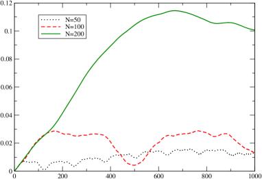
Figure 1: Plot of the rescaled error ${\cal E}_{\rho}(t)$ in $g_{xx}$ for the 1D gauge wave with 10 Dirichlet boundary conditions using the bare ${\hat{W}}$ algorithm (no constraint adjustment or dissipation) obtained with $N=50$, 100 and 200 grid zones. The horizontal axis measures crossing time $t$. The instabilities are kept under control during the entire 1000 crossing times run.

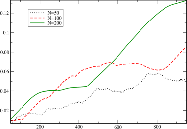
Figure 2: Plot of the rescaled error ${\cal E}_{\rho}(t)$ in $g_{xx}$ for the 1D gauge wave as in Fig. 1 but with 10 Neumann boundary conditions.

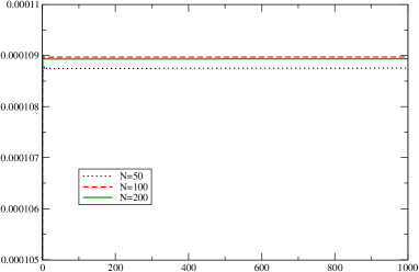
Figure 3: Plot of the rescaled error ${\cal E}_{\rho}(t)$ in $g_{xx}$ for the 1D gauge wave as in Fig. 1 but with 10 Sommerfeld boundary conditions. Excellent performance with clean second order convergence is manifest for 1000 crossing times.

Test results using 3 Dirichlet boundary conditions (for the components $\gamma^{xa}$) and seven Neumann boundary conditions (for the components $\gamma^{xx}$ and $\gamma^{ab}$), with boundary data supplied by the analytical solution, were practically identical to results for the 10 Neumann boundary conditions. When these seven pieces of Neumann boundary data was generated by the constraint preserving boundary system, as detailed in Sec. V.4, practically identical results were again found. This is because no appreciable constraint violation is excited in the shift-free gauge wave test. For the same reason, constraint adjustments have no significant effect.

Two-dimensional tests of the diagonally propagating gauge wave were also in line with expectations. The most important background information for the design of physically relevant boundary algorithms using CCM comes from the case of 10 Sommerfeld boundary conditions and the case of boundary conditions supplied by the constraint preserving (CP) boundary algorithm. In 2D tests of these algorithms, we found the respective convergence rates

$$r_{10S}(10)=2.0005\,,\quad r_{10S}(100)=2.0004$$

$$r_{CP}(10)=2.0482\,,\quad r_{CP}(100)=1.0338$$

measured at 10 and 100 crossing times. The Sommerfeld case maintains clean second order convergence. At 10 crossing times the constraint preserving system also shows clean second order convergence but at 100 crossing times the convergence rate drops to first order due to accumulation of error. The constraint boundary system (68) involves two derivatives of numerically evolved quantities in order to provide a complete set of Neumann data to the code. This introduces high frequency error in the Neumann data. We have not experimented with ways to dissipate this source of error in the boundary system.

VI.2 Shifted gauge wave boundary tests

Simulation of the shifted gauge wave (128) is complicated by the related exponentially growing Kerr-Schild metric babev

$$ds_{\lambda}^{2}=-dt^{2}+dx^{2}+dy^{2}+dz^{2}+\bigg{(}H-1+e^{\lambda\hat{t}}\bigg{)}k_{\alpha}k_{\beta}dx^{\alpha}dx^{\beta},$$ (138)

where

$$\hat{t}=t-\frac{Ad}{4\pi}\cos\left(\frac{2\pi(x-t)}{d}\right).$$ (139)

Although this metric does not solve Einstein’s equations, for any value of $\lambda$ it satisfies the standard harmonic form (4) of the reduced Einstein equations, i.e. the equations upon which the numerical evolution is based. Numerical error in the shifted gauge wave test should be expected to excite this instability. As a result, in shifted gauge wave tests with periodic boundary conditions babev , the constraint adjustment (14) or (15) was necessary to modify the form of the reduced system in order to eliminate the solution (138).

Figures 4, 5 and 6 plot the rescaled error ${\cal E}_{\rho}(t)$ in $g_{xx}$ for shifted gauge wave tests with amplitude $A=.5$ using the bare ${\hat{W}}$ algorithm (no constraint adjustment or dissipation). The results in Fig. 4 for 10 Dirichlet boundary conditions are much less accurate than test results for the bare algorithm reported in babev for periodic boundary conditions. The periodic tests run about 4 times longer with the comparable error. The results for 10 Neumann boundary conditions shown in Fig. 5 are poorer yet by an additional factor of 4 when compared to the periodic tests. These results can be attributed to the periodic motion of the boundary introduced by the shift. As explained in more detail in bab , the numerical noise can be blue shifted as it is reflected at the moving boundaries, leading to rapid build up of error. The results show second order convergence only at early times. For the 10-Dirichlet test we measured the convergence rate $r_{10D}(10)=2.077$ at 10 crossing times. For the 10-Neumann test, we measured the convergence rates $r_{10N}(1)=2.013$, $r_{10N}(5)=2.760$ and $r_{10N}(10)=3.978$, at 1, 5 and 10 crossing times. The high convergence rate at 10 crossing times is misleading since instabilities have already dominated the $N=100$ run (the coarser grid in the convergence calculation).

Figure 6 shows that 10 Sommerfeld boundary conditions gives very good long term performance for the bare algorithm. The accuracy after 1000 crossing times is much better than found in babev for the bare algorithm with periodic boundary conditions, as expected since the Sommerfeld conditions allow numerical error to leave the grid. We measured the convergence rate

$$r_{10S}(50)=2.413$$ (140)

at 50 crossing times.

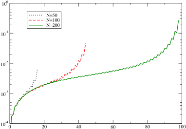
Figure 4: Log plot of the rescaled error ${\cal E}_{\rho}(t)$ in $g_{xx}$ for the 1D gauge wave with shift for the bare $\hat{W}$ algorithm with 10 Dirichlet boundary conditions. Although clean second order convergence is measured at early times, the simulation goes unstable in less than 100 crossing times.

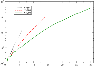
Figure 5: Log plot of the rescaled error ${\cal E}_{\rho}(t)$ in $g_{xx}$ for the 1D gauge wave with shift as in Fig. 4 but with 10 Neumann boundary conditions. Again the runs converge at early times but now the unstable mode is evident at less than 30 crossing times.

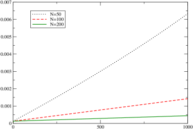
Figure 6: Plot of the rescaled error ${\cal E}_{\rho}(t)$ in $g_{xx}$ for the 1D gauge wave with shift as in Fig. 4 but with 10 Sommerfeld boundary conditions. The error has only a slow linear growth in time.

As we have already pointed out for the case of periodic boundary conditions, although clear second order convergence was established for short run times, good long term performance for the shifted gauge wave tests was only possible when constraint adjustments were used to control the unstable mode (138). The situation is similar in the presence of boundaries. Figure 7 shows the dramatic improvement in performance obtained by using the adjustment (15), with $a_{2}=1$, for 1D tests with 10 Dirichlet boundary conditions, with no dissipation added. The figure shows good second order convergence, with only a small, non-growing error at 1000 crossing times. The convergence rate $r_{10D}(50)=2.018$ was measured at 50 crossing times. For the same adjustment, with no dissipation, Figure 8 shows the test results for 10 Neumann boundary conditions. Again there is very good accuracy for 1000 crossing times, although the error is larger than the Dirichlet case because the boundary conditions now allow the instability (138) to be excited. The convergence rate $r_{10N}(50)=2.877$ was measured at 50 crossing times.

The 1D tests with 10 Sommerfeld boundary conditions already gave good results for the bare algorithm which constraint adjustment or dissipation do not substantially improve. Figure 9 shows the rescaled error for 2D shifted gauge wave tests with the 10-Sommerfeld boundary algorithm. The convergence rates

$$r_{10S,2D}(10)=2.096\,,\quad r_{10S,2D}(100)=2.680\$$ (141)

were measured at 10 and 100 crossing times.

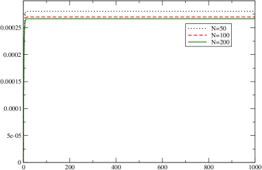
Figure 7: Plot of the rescaled error ${\cal E}_{\rho}(t)$ in $g_{xx}$ for the 1D shifted gauge wave test with 10 Dirichlet boundary conditions as in Fig. 4 but when the adjustment (15) is used. The dramatic improvement compared with Fig. 4 is evident. There is no long term error growth during the 1000 crossing time run.

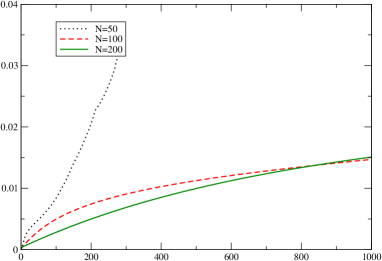
Figure 8: Plot of the rescaled error ${\cal E}_{\rho}(t)$ in $g_{xx}$ for the 1D shifted gauge wave test with 10 Neumann boundary conditions as in Fig. 5 but when the adjustment (15) is used. Again, the adjustment leads to dramatic improvement.

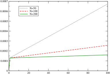
Figure 9: Plot of the rescaled error ${\cal E}_{\rho}(t)$ in $g_{xx}$ with 10 Sommerfeld boundary conditions as in Fig. 6 but now for the 2D shifted gauge wave test. As in the 1D test, the error has only a slow linear growth in time.

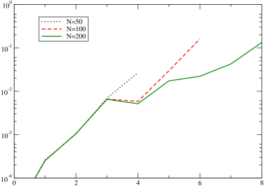
Figure 10: Log plot of the rescaled error ${\cal E}_{\rho}(t)$ in $g_{xx}$ for the 1D shifted gauge wave test with 7 Neumann and 3 Dirichlet boundary conditions and amplitude $A=0.5$. The instabilities which appear in less than 8 crossing times cannot be controlled by dissipation or by the constraint adjustments considered here.

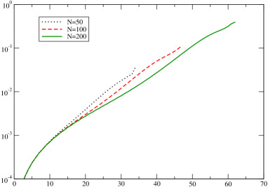
Figure 11: Log plot of the rescaled error ${\cal E}_{\rho}(t)$ in $g_{xx}$ for the 1D shifted gauge wave test with 7 Neumann and 3 Dirichlet boundary conditions as in Fig. 10 but with amplitude $A=.1$.

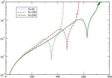
Figure 12: Log plot of the rescaled error ${\cal E}_{\rho}(t)$ in $g_{xx}$ for the 1D shifted gauge wave test with 7 Neumann and 3 Dirichlet boundary conditions as in Fig. 10 but with amplitude $A=.01$. The rapid attenuation of the growth rate of the instability with amplitude is evident from comparison with Fig’s 10 and 11.

The constraint preserving boundary algorithm described in Sec. IV requires 3 Dirichlet boundary conditions (for $\gamma^{xa}$) and 7 Neumann boundary conditions (for $\gamma^{xx}$ and $\gamma^{ab}$). As shown in Fig.10, when the 3 Dirichlet and 7 Neumann pieces of boundary data are supplied by the analytic solution the results for the shifted gauge wave test are very poor due to the early excitation of an unstable error mode. The rescaled error plotted in Fig. 10 shows that good performance is maintained for less than 8 crossing times. The constraint adjustments (14) - (16), as well as other adjustments considered in babev , do not lead to improvement. In particular, the adjustment (15), which works remarkably well in suppressing instabilities in the 10-Dirichlet and 10-Neumann algorithms, fails to be effective when these algorithms are mixed. This seems related to the fact that a Kerr-Schild pulse reflected by 10-Dirichlet or 10-Neumann conditions results in a Kerr-Schild pulse traveling in the opposite direction. When the Dirichlet and Neumann conditions are mixed, the reflected pulse has opposite signs for the Neumann and Dirichlet components. As a result, the reflected pulse no longer has the necessary Kerr-Schild properties for which the adjustment (15) was designed and a new unstable mode is excited. The effect arises from the nonlinear coupling between the Dirichlet and Neumann components and does not arise in the AwA gauge wave test where the Dirichlet components vanish. The new unstable mode has long wavelength so it cannot be controlled by dissipation and it satisfies $Q\approx 0$ (see (72)) so that it cannot be controlled by the semi-discrete conservation law $Q_{,t}=0$.

The effect of the constraint-preserving boundary system on the shifted gauge wave test depends upon the performance of the underlying 3-Dirichlet, 7-Neumann boundary algorithm so it also does not lead to good performance for amplitude $A=.5$. For smaller amplitudes, the instability from the Dirichlet-Neumann mixing is weaker. Figures 11 and 12 show how the rescaled error behaves as the amplitude is lowered to $A=.1$ and $A=.01$, when the Dirichlet-Neumann data is supplied analytically. For the $N=200$ grid and amplitude $A=.01$, reasonable performance is maintained for 500 crossing times.

Only slight improvement is obtained when the constraint preserving boundary system is applied to the 3-Dirichlet, 7-Neumann algorithm. This is apparently because the troublesome instability is a constraint preserving mode. Figures 13 and 14 compare the $\ell_{\infty}$ error norms for constraint violation with and without the application the constraint preserving boundary system for the shifted gauge wave with amplitude $A=.1$. The figures show that both the ${\cal C}^{x}$ and ${\cal C}^{t}$ components of the harmonic constraints are satisfied to much higher accuracy when the constraint preserving boundary system is used. However, the unstable mode still grows on the same time scale and eventually dominates the simulation.

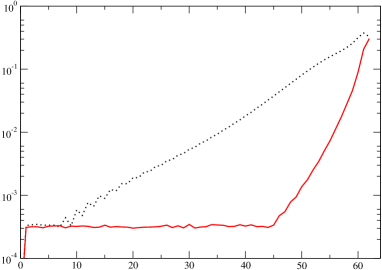
Figure 13: Log plots of the error ${\cal E}_{\rho}(t)$ in the constraint $C^{x}$ for the 1D shifted gauge wave test with amplitude $A=.1$ with 7 Neumann and 3 Dirichlet boundary conditions on an $N=200$ grid. The curve ($\cdot~{}\cdot~{}\cdot$) is the error when the boundary data is supplied analytically and the curve ($---$) is the error when the constraint preserving boundary system is applied.

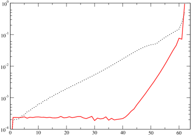
Figure 14: Log plots of the constraint error ${\cal E}_{\rho}(t)$ as in Fig. 13 but for the component $C^{t}$. Although the constraint preserving boundary system ($---$) leads to much less constraint violation, the time scale of the unstable mode is unaffected.

VII Summary and Implications for Cauchy-characteristic matching

We have formulated several maximally dissipative boundary algorithms for well-posed and constraint preserving versions of the general harmonic IBVP. The algorithms incorporate SBP and other semi-discrete conservation laws for the principle part of the system. In boundary tests based upon the AwA gauge wave, we have demonstrated that these techniques give rise to excellent long term (1000 crossing times), nonlinear (amplitude $A=.5$) performance for all boundary algorithms considered. This is an especially challenging test. A high amplitude periodic wave enters one boundary, crosses the computational domain and exits the other boundary. The numerical error modes, which are continously being excited, are trapped between the boundaries by the reflecting Neumann or Dirichlet conditions. However, this causes no serious problem because the chief unstable mode is suppressed by the conservation laws and the growth of error is limited by the dissipation inherent in the system.

The shifted gauge wave boundary test proved even more challenging, as expected from the blue shifting of the error resulting from reflection off the oscillating boundaries. However, 10 Sommerfeld boundary conditions (on the components of the metric) continued to give excellent long term, nonlinear performance. Furthermore, with the use of the constraint adjustment (15), 10 Dirichlet or 10 Neumann boundary conditions also continued to give good long term, nonlinear performance. However, nonlinear instabilities, which did not respond to constraint adjustment, were excited by the mixture of 3 Dirichlet and 7 Neumann boundary conditions. This led to much poorer results and reasonable long term performance required amplitudes $A\leq.01$. When the 3-Dirichlet, 7-Neumann boundary algorithm was amended to include the constraint preserving boundary system, the performance was only slightly improved. The results for this test problem indicate that the mixing of Dirichlet and Neumann boundary conditions excites a nonlinear instability of the analytic problem which cannot be controlled by the numerical techniques considered here.

The above results focused on the mathematical and computational issues underlying accurate long term simulation of the IBVP but they also have bearing on the important physical issue of providing proper boundary data for waveform extraction by means of CCM. In the absence of analytic boundary data, as supplied in the gauge wave testbeds, constraint preserving boundary data must be obtained either by using a constraint preserving boundary system or by matching to an exterior solution which accurately satisfies the constraints. The inaccuracies which we have found in applying the constraint preserving boundary system would only be tolerable in matching with a Cauchy boundary in the weak field regime, i.e. far from the sources. On the other hand, the use of 10 Sommerfeld boundary conditions shows robust long term accuracy even in the strong field regime and would allow the economy of a boundary close to the sources. This is a strong recommendation for a matching algorithm based upon Sommerfeld boundary conditions, with constraint preserving Sommerfeld data supplied by matching to an exterior characteristic solution.

Constraint preservation with a Sommerfeld boundary algorithm in CCM is greatly facilitated by using harmonic evolution. In CCM, there is a Cauchy evolution region with outer boundary ${\cal B}_{O}$ and a characteristic evolution region, extending to ${\cal I}^{+}$, with inner boundary ${\cal B}_{I}$ inside the Cauchy boundary ${\cal B}_{O}$. A global solution is obtained by injecting the necessary Cauchy boundary data on ${\cal B}_{O}$ from the characteristic evolution. In doing so there are two concerns: (i) injection of the Cauchy data in the correct gauge and (ii) injection of constraint-preserving Cauchy data. Harmonic evolution simplifies dealing with both of these concerns because the gauge conditions and constraints reduce to wave equations for the harmonic coordinates $x^{\alpha}$. By extracting data for $x^{\alpha}$ on the inner characteristic boundary ${\cal B}_{I}$, the harmonic coordinates can be accurately propagated by characteristic evolution to the injection worldtube ${\cal B}_{O}$ as solutions of the wave equation. This supplies the necessary Jacobian between the characteristic and Cauchy coordinates to ensure that the above two concerns are properly handled. Furthermore, since such data is constraint-preserving (up to numerical error), it is possible to inject the data in (inhomogeneous) Sommerfeld form. As evidenced by the test results in Sec. VI, this offers a very robust way of injecting boundary data which obeys all the constraints of the harmonic system, while avoiding the computational error introduced by solving the boundary constraint system. This was part of the strategy employed in harl in successfully implementing long term stable CCM in linearized gravitational theory. The results of this paper suggest that this is also a promising approach for carrying out CCM in the nonlinear case.

Appendix A IBVP for a scalar field in a curved background spacetime

The well-posedness of the IBVP for the scalar wave equation with shift can be established by standard techniques by reducing the evolution system to symmetric hyperbolic form. We consider the principle part of the scalar wave equation written in the form

$$g^{\mu\nu}\partial_{\mu}\partial_{\nu}\Phi=0.$$ (142)

We reduce this to the first order symmetric hyperbolic system $A^{t}\partial_{t}u+A^{i}\partial_{i}u=S$, following a treatment in cour , by introducing the auxiliary variables ${\cal T}=\partial_{t}\Phi$, ${\cal X}=\partial_{x}\Phi$, ${\cal Y}=\partial_{y}\Phi$, and ${\cal Z}=\partial_{z}\Phi$. Then in terms of the 5 dimensional column vector $u={}^{T}(\Phi,{\cal T},{\cal X},{\cal Y},{\cal Z})$, the matrices $A^{\alpha}$ are given by

$$A^{t}=\left(\begin{array}[]{ccc}1&0&0\\ 0&-g^{tt}&0\\ 0&0&g^{jk}\end{array}\right)$$ (143)

and

$$A^{i}=\left(\begin{array}[]{ccc}0&0&0\\ 0&-2g^{ti}&-g^{ji}\\ 0&-g^{ij}&0\end{array}\right)$$ (144)

and $S={}^{T}({\cal T},0,0,0,0)$. In this first order form, the Cauchy data consist of $u_{0}=u|_{t=0}$ subject to the constraints

$$({\cal C}_{x},{\cal C}_{y},{\cal C}_{z}):=({\cal X},{\cal Y},{\cal Z})-(\partial_{x}\Phi,\partial_{y}\Phi,\partial_{z}\Phi)=0.$$ (145)

The evolution system implies that the constraints propagate according to

$$\partial_{t}({\cal C}_{x},{\cal C}_{y},{\cal C}_{z})=0.$$ (146)

The well-posedness of the Cauchy problem follows from the established properties of symmetric hyperbolic systems.

We now consider the IBVP in the domain $t\geq 0$ with $x\leq 0$. The constraints propagate up the timelike boundary at $x=0$ and present no complication. The “boundary matrix”

$$A^{x}=\left(\begin{array}[]{ccc}0&0&0\\ 0&-2g^{tx}&-g^{jx}\\ 0&-g^{xj}&0\end{array}\right)$$ (147)

has a 3-dimensional kernel, with a basis corresponding to the vectors

$${}^{T}(1,0,0,0,0),\quad{}^{T}(0,0,-g^{xy},g^{xx},0),\quad\mbox{and}\quad{}^{T}(0,0,-g^{xz},0g^{xx}).$$ (148)

In addition, there is one positive eigenvalue and one negative eigenvalue

$$\lambda_{\pm}=\pm\lambda-g^{xt},$$ (149)

where

$$\lambda=\sqrt{({g^{xt}})^{2}+\delta_{ij}g^{xi}g^{xj}}.$$ (150)

Thus precisely one boundary condition is required. The corresponding normalized eigenvectors are

$$u_{\pm}=\frac{1}{\sqrt{\pm 2\;\lambda\;\lambda_{\pm}}}\;{}^{T}(0,\mp\lambda+g^{xt},g^{xx},g^{xy},g^{xz}).$$ (151)

The homogeneous boundary condition $Mu=0$ may be cast in the form that $u$ lies in the linear subspace $(u_{+}+Hu_{-}+u_{0})$, where $u_{0}$ lies in the kernel. In this subspace, the flux

$${\cal F}^{x}=\frac{1}{2}\,{}^{T}(u_{+}+Hu_{-}+u_{0})A^{x}(u_{+}+Hu_{-}+u_{0})=\lambda_{+}+\lambda_{-}H^{2},$$ (152)

satisfies the dissipative condition ${\cal F}^{x}\geq 0$ provided

$$H^{2}\leq-{\lambda_{+}}\;/\;{\lambda_{-}}\;.$$ (153)

The homogeneous boundary condition corresponding to a choice of $H$ is

$$Mu:={}^{T}(Hu_{+}-u_{-})u=0\;.$$ (154)

The limiting case $H=\sqrt{-\;{\lambda_{+}}\;/\;{\lambda_{-}}}$ leads to the homogeneous Dirichlet boundary condition

$$\partial_{t}\Phi=0$$ (155)

and the limiting case $H=-\sqrt{-\;{\lambda_{+}}\;/\;{\lambda_{-}}}$ leads to the homogeneous Neumann boundary condition

$$g^{\alpha x}\partial_{\alpha}\Phi=0.$$ (156)

As an alternative to this standard eigenvalue analysis of the maximally dissipative boundary condition, the simplicity of the scalar wave case allows a direct geometrical approach. A straightforward calculation gives

$${\cal F}^{x}=\frac{1}{2}\,{}^{T}uA^{x}u=-(\partial_{t}\Phi)g^{x\alpha}\partial_{\alpha}\Phi,$$ (157)

which is identical to the energy flux obtained from the stress-energy tensor of a massless scalar field. It immediately follows that ${\cal F}^{x}=0$ for the above specifications of homogeneous Dirichlet and Neumann boundary conditions. More generally, ${\cal F}^{x}>0$ for boundary conditions of the form $(g^{x\mu}\partial_{\mu}\Phi+P\partial_{t}\Phi)$, with $P>0$. An important case is the choice

$$P=\sqrt{-\frac{g^{xx}}{g_{tt}}}$$ (158)

which leads to the homogeneous Sommerfeld-like boundary condition

$$L^{\mu}\partial_{\mu}\Phi=g^{x\mu}\partial_{\mu}\Phi+\sqrt{-\frac{g^{xx}}{g_{tt}}}\partial_{t}\Phi=0,$$ (159)

where $L^{\mu}$ lies in the outgoing null direction in the $(t^{\alpha},\nabla^{\alpha}x)$ plane.

The well-posedness of the IBVP for the scalar wave equation with any of the above choices of maximally dissipative boundary condition extends, by Secchi’s theorem secchi2 , to the quasilinear reduced Einstein equations (69). The extension of the homogeneous boundary condition $Mu=0$ to include free boundary data $q$ takes the form $M(u-q)=0$. For example, the Neumann boundary condition (156) takes the inhomogeneous form $g^{\alpha x}\partial_{\alpha}\Phi=q$, where the boundary data $q$ can be freely assigned. The well-posedness of the IBVP for the wave equation with inhomogeneous boundary data follows from the well-posedness of the homogeneous case by a standard argument.

Appendix B Extrinsic curvature

The extrinsic curvature tensor of the boundary at $x=0$ (of the domain $x\leq 0$) is given by

$$K^{\mu\nu}=h^{\mu}_{\alpha}h^{\nu}_{\beta}\nabla^{\alpha}n^{\beta}$$ (160)

where

$$h_{\alpha}^{\mu}=\delta_{\alpha}^{\mu}-n_{\alpha}n^{\mu}$$ (161)

is the projection tensor into the tangent space of the boundary and $n_{\alpha}=(1/\sqrt{g^{xx}})\nabla_{\alpha}x$ is the unit outward normal. In the 3+1 decomposition $x^{\mu}=(x^{a},x)$, $h_{ab}$ is the intrinsic metric of the boundary, $h_{\mu}^{x}=0$, $h_{\mu b}=g_{\mu b}$ and $h_{xx}=g_{xx}-(1/g^{xx}$.) Also note that $h_{\cal B}=det(h_{ab})=g^{xx}g$.

We set $n^{\mu}=\sqrt{g^{xx}}q^{\mu}=\sqrt{g^{xx}}(q^{a},1)$, where $q^{a}=\gamma^{xa}/\gamma^{xx}$. In terms of the metric,

$$K^{\mu\nu}=\frac{\sqrt{g^{xx}}}{2}h^{\mu}_{\alpha}h^{\nu}_{\beta}(g^{\alpha\rho}\partial_{\rho}q^{\beta}+g^{\beta\rho}\partial_{\rho}q^{\alpha}-q^{\rho}\partial_{\rho}g^{\alpha\beta}).$$ (162)

In expressing this in terms of $\gamma^{\mu\nu}$, the identity

$$\partial_{\alpha}g=-\sqrt{-g}g_{\mu\nu}\partial_{\alpha}\gamma^{\mu\nu}$$ (163)

is useful. For example,

$$\partial_{x}g^{\mu\nu}=\frac{1}{\sqrt{-g}}(\partial_{x}\gamma^{\mu\nu}-\frac{1}{2}g^{\mu\nu}g_{\alpha\beta}\partial_{x}\gamma^{\alpha\beta}).$$ (164)

As a result,

$$K^{\mu\nu}=\frac{\sqrt{g^{xx}}}{2}(h^{\mu\rho}h^{\nu}_{\beta}\partial_{\rho}q^{\beta}+h^{\mu}_{\alpha}h^{\nu\rho}\partial_{\rho}q^{\alpha})-\frac{g^{xx}}{2\sqrt{-h}}(h^{\mu}_{\alpha}h^{\nu}_{\beta}q^{\rho}\partial_{\rho}\gamma^{\alpha\beta}-\frac{1}{2}h^{\mu\nu}g_{\lambda\tau}q^{\rho}\partial_{\rho}\gamma^{\lambda\tau})$$ (165)

and

$$K^{\mu\nu}-h^{\mu\nu}K = \frac{\sqrt{g^{xx}}}{2}(h^{\mu\rho}h^{\nu}_{\beta}\partial_{\rho}q^{\beta}+h^{\mu}_{\alpha}h^{\nu\rho}\partial_{\rho}q^{\alpha}-2h^{\mu\nu}h^{\rho}_{\beta}\partial_{\rho}q^{\beta})$$ (166)

$$- \frac{g^{xx}}{2\sqrt{-h}}(h^{\mu}_{\alpha}h^{\nu}_{\beta}q^{\rho}\partial_{\rho}\gamma^{\alpha\beta}+h^{\mu\nu}n_{\alpha}n_{\beta}q^{\rho}\partial_{\rho}\gamma^{\alpha\beta}).$$

The boundary version of the usual momentum constraint implies

$$h^{\mu}_{\sigma}n_{\nu}G^{\sigma\nu}=D_{\nu}(K^{\mu\nu}-h^{\mu\nu}K),$$ (167)

where $D_{a}$ is the covariant derivative associated with the boundary metric $h_{ab}$. We express this “boundary momentum” in the 3-dimensional form of the $x^{a}=(t,x,y)$ coordinates:

$$h^{a}_{\sigma}n_{\nu}G^{\sigma\nu}=D_{b}(K^{ab}-h^{ab}K)=0.$$ (168)

The identity

$$\sqrt{-h_{\cal B}}D_{b}S_{a}^{b}=\partial_{b}(\sqrt{-h_{\cal B}}S_{a}^{b})-\frac{1}{2}\sqrt{-h_{\cal B}}S^{bc}\partial_{a}h_{bc},$$ (169)

valid for any symmetric tensor $S^{bc}$, is useful in calculating the covariant derivatives entering the constraint.

- (1) R. Penrose, “Asymptotic properties of fields and space-times”, Phys. Rev. Lett. 10, 66 (1963).
- (2) S. Husa, “Numerical relativity with the conformal field equations”, Lect. Notes Phys., 617, 159 (2003).
- (3) J. Frauendiener, “Conformal infinity”, Living Rev. Relativity 7 (2004).
- (4) J. Winicour, “Characteristic evolution and matching”, Living Rev. Relativity 8, 10 (2005).
- (5) N. T. Bishop, R. O. Gómez, R. A. Isaacson, L. Lehner, B. Szilágyi, and J. Winicour, “Cauchy-characteristic matching”, in Black Holes, Gravitational Radiation and the Universe, eds. B. Bhawal, B. and B. R. Iyer, (Kluwer,Dordrecht, 1998).
- (6) B. Szilágyi and J. Winicour, “Well-posed initial-boundary evolution in general relativity”, Phys. Rev. D68, 041501 (2003).
- (7) H. Friedrich and A. D. Rendall, “The Cauchy problem for the Einstein equations”, in Einstein’s Field Equations and Their Physical Implications: Selected Essays in Honour of Jürgen Ehlers, ed. B. G. Schmidt, Springer, Berlin (2000).
- (8) J. M. Stewart, “The Cauchy problem and the initial boundary value problem in numerical relativity”, Class. Quantum Grav. 15, 2865 (1998).
- (9) H. Friedrich and G. Nagy, Commun. Math. Phys., 201, 619 (1999).
- (10) B. Szilágyi, R. Gomez, N. T. Bishop and J. Winicour, “Cauchy boundaries in linearized gravitational theory”, Phys.Rev. D62 104006 (2000).
- (11) B. Szilágyi, B. G. Schmidt and J. Winicour, Boundary conditions in linearized harmonic gravity, Phys. Rev. D65, 064015 (2002).
- (12) C. Calabrese, L. Lehner and M. Tiglio, “Constraint-preserving boundary conditions in numerical relativity”, Phys. Rev. D65, 104031 (2002).
- (13) C. Calabrese, J. Pullin, O. Reula, O. Sarbach and M. Tiglio, “Well posed constraint-preserving boundary conditions for the linearized Einstein equations”, Commun. Math. Phys. 240, 377 (2003).
- (14) C. Calabrese and O. Sarbach, “Detecting ill posed boundary conditions in General Relativity”, Commun. Math. Phys. 240, 377 (2003). J. Math. Phys. 44, 3888 (2003).
- (15) S. Frittelli and R. Gómez, “Einstein boundary conditions for the 3+1 Einstein equations”, Phys. Rev. D68, 044014 (2003).
- (16) S. Frittelli and R. Gómez, “Boundary conditions for hyperbolic formulations of the Einstein equations”, Class. Quant. Grav. 20, 2739 (2003).
- (17) M. C. Babiuc, B. Szilágyi and J. Winicour, “Some mathematical problems in numerical relativity”, Lect. Notes Phys. (to appear) gr-qc/0404092.
- (18) S. Frittelli and R. Gómez, ‘Einstein boundary conditions for the Einstein equations in the conformal-traceless decomposition‘”, Phys. Rev. D70,064008 (2004).
- (19) O. Sarbach, and M. Tiglio,“Boundary conditions for Einstein’s equations: Analytical and numerical analysis”, gr-qc/0412115.
- (20) C. Gundlach and J. M. Martin-Garcia, “Symmetric hyperbolicity and consistent boundary conditions for second-order Einstein equations”, Phys. Rev. D70, 044032 (2004).
- (21) L. E. Kidder, L. Lindblom, M. A. Scheel, L. T. Buchman and H. P. Pfeiffer, “Boundary Conditions for the Einstein Evolution System”, Phys.Rev. D71, 064020 (2005).
- (22) C. Bona, T. Ledvinka, C. Palenzuela-Luque and M. Zacek, “Constraint-preserving boundary conditions in the Z4 Numerical Relativity formalism”, Class. Quant. Grav. 22, 2615 (2005).
- (23) L. Lehner, O. Reula, and M. Tiglio, “Multi-block simulations in general relativity: high order discretizations, numerical stability, and applications”, gr-qc/0507004.
- (24) G. Calabrese and C. Gundlach, “Discrete boundary treatment for the shifted wave equation”, gr-qc/0509119.
- (25) L. Lindblom, M. A. Scheel, L. E. Kidder, R. Owen and and O. Rinne, “A New Generalized Harmonic Evolution System”, gr-qc/0512093.
- (26) Y. Foures-Bruhat, “Theoreme d’existence pour certain systemes d’equations aux deriveés partielles nonlinaires”, Acta Math 88, 141 (1952).
- (27) F. Pretorius, “Numerical Relativity Using a Generalized Harmonic Decomposition”, Class. Quant. Grav. 22, 425 (2005).
- (28) F. Pretorius, “Evolution of Binary Black Hole Spacetimes”, Phys.Rev.Lett., 95, 121101 (2005).
- (29) V. Fock,The Theory of Space, Time and Gravitation, (MacMillan, New York, 1964).
- (30) R. M. Wald, “General Relativity”, University of Chicago Press (1984).
- (31) M. C. Babiuc, B. Szilágyi and J. Winicour, “Testing numerical evolution with the shifted gauge wave”, gr-qc/0511154.
- (32) H. Friedrich, “Hyperbolic reductions for Einstein’s equations”, Class. Quant. Grav., 13, 1451 (1996).
- (33) The AppleswithApples Alliance, M. Alcubierre et al, “Towards standard testbeds for numerical relativity”, Class. Quantum Grav., 21, 589 (2004).
- (34) B. Szilágyi, H-O. Kreiss and J. Winicour, “Modeling the black hole excision problem”, Phys. Rev. D71, 104035 (2005).
- (35) C. Gundlach, J. M. Martin-Garcia, G. Calabrese and I. Hinder, “Constraint damping in the Z4 formulation and harmonic gauge”, Class. Quant. Grav. 22, 3767 (2005).
- (36) M. Alcubierre and B. Schutz, J. Comput. Phys., 112, 44 (1994).
- (37) G. Calabrese, “Finite differencing second order systems describing black hole spacetimes”, Phys.Rev. D 71, 027501 (2005).
- (38) M. Tiglio, L. Lehner and D. Neilsen, “3D simulations of Einstein’s equations: symmetric hyperbolicity, live gauges and dynamic control of the constraints” Phys. Rev D70, 104018 (2004).
- (39) L. Lehner, D. Neilsen, O. Reula and M. Tiglio, “The discrete energy method in numerical relativity: Towards long-term stability” Class. Quant. Grav. 21 5819 (2004).
- (40) G. Calabrese, L. Lehner, O. Reula, O. Sarbach, M. Tiglio, “Summation by parts and dissipation for domains with excised regions”, Class. Quant. Grav. 21, 5735 (2004).
- (41) P. Secchi, Arch. Rational Mech. Anal., 134, 595 (1996).
- (42) R. Courant and D. Hilbert, Methods of Mathematical Physics, Vol. II, p. 594 (Interscience, NY, 1962).