Darwin Meets Einstein: LISA Data Analysis Using Genetic Algorithms

Abstract

This work presents the first application of the method of Genetic Algorithms (GAs) to data analysis for the Laser Interferometer Space Antenna (LISA). In the low frequency regime of the LISA band there are expected to be tens of thousands galactic binary systems that will be emitting gravitational waves detectable by LISA. The challenge of parameter extraction of such a large number of sources in the LISA data stream requires a search method that can efficiently explore the large parameter spaces involved. As signals of many of these sources will overlap, a global search method is desired. GAs represent such a global search method for parameter extraction of multiple overlapping sources in the LISA data stream. We find that GAs are able to correctly extract source parameters for overlapping sources. Several optimizations of a basic GA are presented with results derived from applications of the GA searches to simulated LISA data.

I Introduction

The Laser Interferometer Space Antenna (LISA) PrePhaseA is set to be launched in the middle of the next decade. As LISA is an all-sky antenna, it will detect sources in all directions, and across a great range of distances. The types of sources range from monochromatic white dwarf binaries in our own galaxy to rapidly coalescing supermassive black hole binaries in the distant reaches of the Universe. The challenge for analyzing the LISA data stream will be pulling out the various parameters of as many of these sources as is possible. A large impediment to completing this challenge is the many thousands of low frequency, effectively monochromatic sources evans ; lip ; hils ; hils2 ; gils that will be present in the LISA data streams. Extracting the parameters from so many sources at once is analogous to determining what every member in the audience of a rock concert is saying. As more sources overlap the confusion grows rapidly source_conf . The name given to this issue is ‘The Cocktail Party Problem’ (see Ref. MCMC for a detailed discussion).

With so many sources, it will be impossible to extract the individual source parameters for every source in the LISA band. This will leave a background of sources whose indeterminable signals blend together into a confusion limited background. Several studies hils ; hils2 ; gils ; sterl ; seth ; bc have indicated that the confusion noise may dominate instrument noise at the low end of the LISA frequency range, so that other sources of interest may be buried beneath the confusion background. For this reason a key goal of LISA data analysis is to reduce the level of the confusion noise as much as possible.

Previous approaches to the extraction of parameters from the LISA data stream have used several methods. Grid based template searches using optimal filtering provide a systematic method to search through all possible combinations of gravitational wave sources, but the computational cost of such a search appears to make it unfeasible temp_grid . Other techniques applied to simulated LISA data involve iterative refinement of a sequential search of sources gclean ; slicedice , a tomographic approach mohanty , global iterative refinement, and ergodic exploration of the parameter space such as Markov Chain Monte Carlo (MCMC) methods MCMC . At this time, however, it is not clear which of these techniques, or which combination of techniques will provide the best solution to the Cocktail Party Problem.

Here we present the first application of the method of genetic algorithms holland to the challenge of extracting parameters from a simulated LISA data stream containing multiple monochromatic gravitational wave sources. The strength of this method lies in its searching capabilities, and thus GAs might be used as the first step in dealing with the confusion background. The initial solution could then be handed off to a MCMC algorithm MCMC , which specializes in determining the nature of the posterior distribution function.

In section II we explore various factors that influence the performance of a genetic search algorithm. A bare-bones algorithm is introduced in II.1, and succeeding layers of complexity are added to this algorithm in II.2 through II.8, with an emphasis on developing an efficient algorithm, which is robust enough to handle the entire low frequency regime of the LISA detector. Applications of the advanced algorithms to multiple source cases are shown in II.7. We conclude with a discussion of future improvements and plans for the application of genetic algorithms to LISA data analysis.

II Genetic Search Algorithms

The fundamental idea behind a genetic algorithm is the survival of the fittest. It is because of this that genetic algorithms are often referred to as evolutionary algorithms, though Darwin origin would probably have considered GAs as “Variation under Domestication” since we are breeding toward a predetermined goal. Through the process of continually evolving solutions to the given problem, genetic algorithms provide a means to search the large parameter space that we will be confronted with in the low frequency region of the LISA band.

A few definitions are in order before delving into our applications of genetic algorithms to LISA data analysis. These definitions will refer to a hypothetical search of the LISA data stream for $N$ monochromatic gravitational wave sources. The search will take advantage of the F-statistic to reduce the search space to $3N$ parameters. The hypothetical search will also involve the use of $n$ simultaneous, competing solution sets.
An organism is a particular $3N$ parameter set that is a possible solution for the source parameters.
A gene is an individual parameter within an organism.
A generation is the set of all $n$ concurrent organisms.
Breeding or cross-over is the process through which a new organism is formed from one or more organisms of the previous generation.
Mutation is a process which allows for variation of a organism as it is bred from the organisms of the previous generation.
Elitism is the technique of carrying over one or more of the best organisms in one generation to the next generation.

A simplified genetic algorithm begins with a set of $n$ organisms that comprise the first generation. The genes of this generation may be chosen at random or selected through some other process. The organisms of each generation are checked for fitness, and those with the best fitness are more likely to breed, with mutation, to form the organisms of the next generation. With passing generations the organisms tend toward better solutions to the source parameters. We use the F-statistic to measure the fitness of each organism.

II.1 Basic Implementation

For our investigations source frequencies were chosen to lie within the range $f\in[0.999995,1.003164]$ mHz. This range spans $100$ frequency bins of width $\Delta f=1/{\rm year}$. Amplitudes were restricted to the range $A\in[10^{-23},10^{-21}]$. By use of the F-statistic our searches are reduced to frequency $f$, and sky location $\theta$ and $\phi$. For a detailed description of the F-statistic and its use in reducing the search space see Refs. fstat ; MCMC .

A simple approach is to represent the values of each search parameter with binary strings. The length of the strings determines the precision of the search, e.g. representing $\theta$ with a binary string of $8$ digits gives precision to $0.7^{\circ}$. Resolution is given by, (parameter range)/$2^{L}$, where $L$ is the length of the binary string. Such a binary representation allows for ease of mutation and breeding. We employed binary strings of length $L=16$ for $f$, $L=13$ for $\theta$ and $L=14$ for $\phi$.

In this basic scheme, we first mutate the parent’s parameter strings, and then breed the mutated gametes. Simple mutation consists of flipping the binary digits of the parent’s parameter strings with probability PMR, the parameter mutation rate. A large PMR will tend to result in more variation in the gametes, and thus the offspring, while a small PMR will lessen variation, resulting in more offspring that resemble their parents.

We use a breeding pattern known as $1$-point crossover, which consists of the combination of complimentary sections of the binary strings of two parent organisms. The cross-over point can be chosen at random or fixed in advance. We chose a fixed cross-over with the cross-over point occurring at the midpoint of the strings. As an example we show the breeding of a parameter represented by strings that are $8$ digits long.

Table 1: Midpoint crossover for an 8 bit string

Parent $1$	$0100$	$1110$
Parent $2$	$0011$	$0011$
Offspring	$0011$	$1110$

We will start with a basic search using $10$ organisms in each generation. The first generation has the genes of its organisms chosen at random from their respective ranges. The probability of each of these organisms being chosen for reproduction is proportional to its likelihood, $\cal L$ (known as fitness proportionate cross-over). Mutated gametes are formed using a PMR of $0.04$, and are bred using a single midpoint crossover.

Figure 1 shows trace plots of the log likelihood, frequency, $\theta$, and $\phi$ for a source with ${\rm SNR}=15.4464$ and parameters: $A=1.97703\times 10^{-22}$, $f=1.000848032$ mHz, $\theta=1.2713$, $\phi=5.34003$, $\iota=2.73836$, $\psi=1.43093$, and $\gamma_{o}=5.59719$ (it is this source that will be used repeatedly throughout the paper). The plotted values were for the organism with the best fit in each generation. As can be seen the parameters are well determined with even this basic scheme, though the noise in the data stream pushes them off their true values. The parameter values are shifted by $\delta f=-1.5\times 10^{-9}$ Hz, $\delta\theta=2.9^{\circ}$ and $\delta\phi=-1.5^{\circ}$ from their input values. These shifts are consistent with the error predictions from a Fisher matrix analysis: $\Delta f=1.7\times 10^{-9}$ Hz, $\Delta\theta=3.5^{\circ}$ and $\Delta\phi=1.9^{\circ}$. The cost of the search is measured in terms of the number of calls to the F-statistic routine and is given by $\$=n\times g$, where $g$ is the generation number. Typical runs of our basic genetic algorithm cost $\$=32650$ calls. This should be compared to a grid based search across the same frequency range, which, for a minimal match of ${\rm MM}=0.9$, would require $\$=110,000$ calls to the F-statistic routine (this value is $2^{3/2}$ larger than that quoted in Ref. MCMC as our earlier calculations used a noise level that was $\sqrt{2}$ larger than the LISA baseline due to a mix up between one and two sided noise spectral densities).

Figure 1: Basic Algorithm: Trace plots for (a) log likelihood, (b) frequency, (c), $\theta$, and (d) $\phi$ for the basic implementation of a genetic algorithm. The y-axes are the parameter values and log likelihoods of the best fit organism for each generation. The x-axes are generation number.

While the basic algorithm is sufficient for finding a solution, it is not efficient. Next we will discuss adjustments to the algorithm that will improve its efficiency, and make it considerably cheaper than a grid based search.

II.2 Aspects of Mutation

In the previous example the PMR was set at the fairly low value of $0.04$. Figure 2 shows trace plots for the same search, but with ${\rm PMR}=0.1$. While the ${\rm PMR}=0.04$ example shows a tendency for small deviations from the improving solutions, the larger PMR search allows large swings in the solution away from a good fit to the true source parameters. On the other hand, Figure 3 shows how a small PMR ($0.001$) can cause the rate of progress to be greatly slowed. A small mutation rate slows the exploration of the likelihood surface.

As these examples show, choosing the proper PMR can have a significant effect on the efficiency of the algorithm. Knowing which value is the proper choice a priori is impossible. Furthermore, at different phases of the search, different values of the PMR will be more efficient than those same values at other phases. Early on in the search a large PMR is desirable for increased exploration. Once convergence to the solution has begun, a smaller PMR is preferable, to prevent suddenly mutating away from the solution. One can imagine a process which changes the PMR in a manner analogous to the simulated annealing process, where we start the PMR high (hot) and lower (cool) it in succeeding generations. In fact, this process in sometimes called simulated annealing in the GA literature. Figure 4 shows trace plots for the same source, using a genetic (PMR) simulated annealing scheme given by:

$${\rm PMR}=\left\{\begin{tabular}[]{ll}${\rm PMR}_{\rm f}\left(\frac{PMR_{\rm i}}{PMR_{\rm f}}\right)^{\frac{g_{\rm cool}-g}{g_{\rm cool}}}$&$0<g<g_{\rm cool}$\\ ${\rm PMR}_{\rm f}$&$g\geq g_{\rm cool}$\end{tabular}\right.$$ (1)

where ${\rm PMR}_{\rm i}=0.2$, ${\rm PMR}_{\rm f}=0.01$, $g$ is the generation number, and $g_{\rm cool}=1000$ is the last generation of the cooling process. The best choice of values for this scheme is again impossible to know a priori. In section II.6 we will see how “Genetic Genetic Algorithms” are able to provide a natural solution to this problem.

Figure 2: Large Mutation Rate: Trace plots for (a) log likelihood, (b) frequency, (c), $\theta$, and (d) $\phi$ for the basic implementation of a genetic algorithm with ${\rm PMR}=0.1$. The y-axes are the parameter values and log likelihoods of the best fit organism for each generation. The x-axes are generation number.

Figure 3: Small Mutation Rate: Trace plots for (a) log likelihood, (b) frequency, (c), $\theta$, and (d) $\phi$ for the basic implementation of a genetic algorithm with ${\rm PMR}=0.001$. The y-axes are the parameter values and log likelihoods of the best fit organism for each generation. The x-axes are generation number.

Figure 4: Genetic Simulated Annealing: Trace plots for (a) log likelihood, (b) frequency, (c), $\theta$, and (d) $\phi$ for the basic implementation of a genetic algorithm with the inclusion of genetic simulated annealing. The y-axes are the parameter values and log likelihoods of the best fit organism for each generation. The x-axes are generation number.

II.3 The effect of the number of organisms on efficiency

While choosing the PMR is one degree of freedom in our basic schema, another is the number of organisms used in the search. Here we look at how the choice of the number of organisms effects the efficiency of the algorithm. The efficiency is inversely related to the computational cost $, which is measured by the number of calls to the function calculating the F-statistic (where the bulk of calculations for an organism are performed), which occurs once per newly formed organism. For example, in Figure 1 there are $10$ organisms in the search and the search surpasses the true parameter log likelihood value at $3851$ generations. Thus its computational cost is $\$=38510$ (function calls).

The data in Figure 5 shows the interplay of the number of organisms with the PMR (held constant within each data run) and their effects on the computational cost. We would expect that relatively large PMRs would be less efficient as was seen in subsection II.2 (and will show up in Figure 7). The size of the effect, however, is modified by the number of organisms in the search. For example, one can find from Figure 5 that the minimum cost ($\$=4492$) for a $20$ organism search occurs when ${\rm PMR}=0.1$, however for $400$ organisms in the search the minimum cost ($\$=7490$) is at ${\rm PMR}=0.14$.

The addition of more organisms in the search provides a kind of stability to the system that decreases the chances of mutating away from good solutions. With just a handful of organisms, and a large PMR, the chances are higher of each organism undergoing a large mutation in at least one parameter. However, with hundreds of organisms the probability of all organisms undergoing such a mutation drops appreciably. Then in the succeeding generation, those organisms that remained a good fit are much more likely to breed the offspring of the next generation. However, this does not hinder great leaps forward. To illustrate this point we will use the data shown in Figure 1. In going from the $7^{th}$ to the $8^{th}$ generation the value of the likelihood of the best fit organism jumps from $1.48\times 10^{13}$ to $6.02\times 10^{20}$. As the probability of breeding is set by the value of the organism likelihood, that new best fit organism is going to be the primary breeder of the next generation (though it is possible that a second organism has also jumped to a point in parameter space with a similar likelihood value).

Increasing the number of organisms not only provides this stabilizing effect, it also provides more chances per generation for improvements due to mutations. One cannot, however, simply throw more organisms at the problem without paying a price; that price will be an eventual drop in efficiency. As an extreme example, imagine using the basic scheme describe in II.1 and putting $40000$ organisms into the search. Even if one of the randomly chosen organisms matched the best fit parameters, the computational cost ($\$=40000$) is already larger than the cost of using $10$ organisms ($\$=38510$). Figure 5 provides a snapshot of the how this choice effects efficiency.

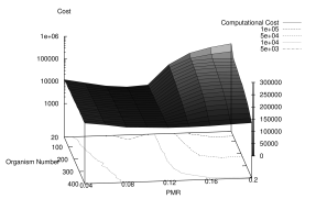
Figure 5: Average Computational Cost as a function of PMR and the number of organisms. The z-axes is the average computational cost calculated from $1000$ searches.

II.4 Elitism

Elitism is akin to cloning. It allows for a perfect copy of an organism or organisms to be bred into the next generation. Including elitism is another way to provide a stabilizing force across generations. This allows for a larger PMR to enhance exploration without the danger of moving off the best fit solution.

Figure 6 shows trace plots for the nominal source with ${\rm PMR}=0.1$ and a single elite organism being cloned at each generation. As expected there is increased exploration (compared to results shown in Figure 1) due to the larger PMR, but unlike the results shown in Figure 2, convergence is now helped by the cloned organism.

Figure 6: Elitism: Trace plots for (a) log likelihood, (b) frequency, (c), $\theta$, and (d) $\phi$ for the basic implementation of a genetic algorithm with ${\rm PMR}=0.1$ and single organism elitism. The y-axes are the parameter values and log likelihoods of the best fit organism for each generation. The x-axes are generation number.

Figure 7 shows a plot relating the average computational cost to the PMR for the case of no elitism, and the case where a single organism is cloned. Computational cost is now derived from the average number of newly formed organisms (note: a cloned organism does not increase computational cost, as all of its associated values are already known). The plot shows the average computational cost of $100$ searches, using $20$ organisms, of a given source (${\rm SNR}=19.2335$ and parameters: $A=1.61486e-22$, $f=1.003$ mHz, $\theta=0.8$, $\phi=2.14$, $\iota=0.93245$, $\psi=2.24587$, and $\gamma_{o}=5.29165$). As was expected, elitism has allowed for a larger PMR, compared to the zero elitism case, increasing the parameter space exploration without sacrificing efficiency.

Figure 7: Average Computational Cost for no elitism and single organism elitism. Data points are determined by the average of $100$ distinct searches.

If one decides to use elitism there is the additional choice of how many elite organisms will be cloned at each generation. At one extreme all organisms are cloned, in which case there is no exploration beyond the first generation. At the other extreme of no elitism the algorithm is unstable against large PMR values, as was seen in Figure 2. There is a balance to be struck between the amount of elitism and the size of the PMR that will provide the most efficient scheme, but the exact nature of the balance can depend on the nature of the search. We describe a solution to this problem in II.6.

II.5 Simulated Annealing

Simulated annealing is a technique that effectively makes the detector more noisy, thus lessing the range of the likelihood function. This increases the probability of choosing poorer sources for reproduction, which allows for a more thorough exploration of the likelihood surface. Think of the likelihood as a partition function $Z=C\exp(-\beta E)$, in which the role of the energy is played by the log likelihood, $E=(s-h|s-h)$, and $\beta$ plays the role of the inverse temperature. Heating up the system (lowering $\beta$) lowers the likelihood range, providing for increased exploration. Starting hot, we use a power law cooling schedule given by:

$$\beta=\left\{\begin{tabular}[]{ll}$\beta_{0}\left(\frac{1}{2\beta_{0}}\right)^{g/g_{\rm cool}}$&$0<g<g_{\rm cool}$\\ $\frac{1}{2}$&$g\geq g_{\rm cool}$\end{tabular}\right.$$ (2)

where $\beta_{0}$ is the initial value of the inverse temperature, $g$ is the generation number, and $g_{\rm cool}$ is the last generation of the cooling process (subsequent generations have $\beta=1/2$). As the likelihood is a sharply peaked function, we found for a single source an initial value of $\beta_{0}\sim 1/100$ was sufficient to speed the process. For multiple source searches increasing that by factors of $3$ to $5$ produced more efficient explorations. Similarly, for multiple sources an increase in $g_{\rm cool}$ was needed to properly explore the surface. This increase scaled roughly linearly with the number of sources.

This mode of simulated annealing, which will be referred to as standard simulated annealing, is markedly different than the genetic version of simulated annealing discussed in II.2. Standard simulated annealing alters the search space, using the heat/energy to smooth the likelihood surface, whereas in genetic simulated annealing the search space was left unchanged and the heat/energy of the organisms was increased via the larger PMRs.

Figure 8 shows trace plots of the log likelihood, frequency, $\theta$, and $\phi$ searching for the same source as in Figure 4. The only change between the two examples is the type of annealing process. For this run ${\rm PMR}=0.04$, $\beta_{0}=1/100$, and $g_{\rm cool}=300$.

Figure 8: Standard Simulated Annealing: Trace plots for (a) log likelihood, (b) frequency, (c), $\theta$, and (d) $\phi$ for the basic implementation of a genetic algorithm with the inclusion of standard simulated annealing and ${\rm PMR}=0.04$. The y-axes are the parameter values and log likelihoods of the best fit organism for each generation. The x-axes are generation number.

II.6 Giving more control to the algorithm

In the previous examples, choices were required as to what PMR or which degree of elitism should be used with a particular source to provide the most efficient search. In making those choices, we are searching for a solution that depends on the information in the data stream. Just as we use the power of the genetic algorithm to search for the parameters of the gravitational wave sources that contribute to the data stream, we can also use that same power to search for efficient values for PMR or elitism.

Treating the PMR, elitism, or other factors in the genetic algorithm like a source parameter these factors can be elevated, or one might say demoted, to the same level as the source parameters. We mentioned this at then end of subsection II.2 and have implemented this idea for the PMR. The initial PMR for each organism is chosen randomly, and the PMR for each organism in the next generation is bred just as $f$, $\theta$, and $\phi$ are, based on organism fitness. This changes the nature of the algorithm from a simple genetic algorithm to a genetic-genetic algorithm (GGA), in which a factor, or factors, determining the search for the source parameters evolve along with the organisms.

Figure 9 shows trace plots for a GGA with the PMR evolving with the organisms. This run includes the simulated annealing scheme used in the previous example and elitism of the single best fit organism. Figure 10 shows the evolution of the PMR for the same run. The ‘genetic simulated annealing’ scheme is visible in the plot with the larger PMRs more efficient earlier on, and smaller PMRs dominating in the later stages. As the evolving PMR values range over nearly two orders of magnitude, it is easy to see why a single, constant choice for the PMR would be so much less efficient. Also, as one can see from the data presented, the variations in the frequency are significantly smaller than those of $\theta$ and $\phi$. We can extend the idea of tailored PMRs beyond the organism, and down to the gene. Giving a separate PMR to each parameter will allow for even better adaptation. (In the natural world organisms control their mutation rates by building in DNA repair mechanisms to counteract the externally determined mutation rate set by cosmic rays and other pathogens).

Figure 9: Genetic-Genetic Algorithm: Trace plots for (a) log likelihood, (b) frequency, (c), $\theta$, and (d) $\phi$ for a genetic-genetic algorithm in which the PMR evolves with the organisms. The y-axes are the parameter values and log likelihoods of the best fit organism for each generation. The x-axes are generation number.

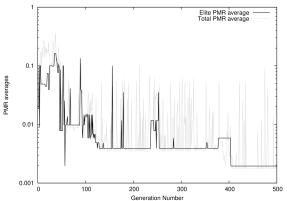
Figure 10: Genetic-Genetic Simulated Annealing of the PMR: Trace plots for the PMR as it evolves with the organisms. The data for this plot is from the same run that produced the data in Figure 9.

II.7 Multiple sources in the data stream

At the low end of the LISA band there will be many thousands of sources. Thus, we expect to see multiple sources even in small segments of the data stream such as the one we have been considering. Simulations point to bright source densities of up to one source per five modulation frequency bins ($f_{\rm mod}=1/{\rm year}$) seth . Thus, any search algorithm must be able to perform multiple source searches at the low end of the LISA band.

Figure 11 shows an implementation of the GGA with standard simulated annealing to a LISA data stream snippet of width $100f_{\rm mod}$, containing five monochromatic binary systems. The standard simulated annealing was completed in the first $g_{\rm cool}=4000$ generations, by which time the GGA had separated out the values for the source frequencies and co-latitudes. The grouping of azimuthal angles was separated soon thereafter, with minor modifications of the parameters occurring over the next $5000$ generations. Search results are summarized in Table 2. The GGA accurately recovered the source parameters in this and similar multiple ($3-5$) source data sets, converging to a best fit solution in less than $5000$ generations per source with $10$ organisms per generation, so long as the source correlation coefficients were below $\sim 0.25$. The intrinsic parameters for the sources were recovered to within $2\sigma$ of the true parameters (based on a Fisher Information Matrix estimate of the uncertainties of the recovered parameters). When highly correlated sources are used, the GGA spends a correspondingly longer time to pick out the source parameters. Investigations in this area were limited. A full study of the affect of source correlation on computational cost is to be carried out in the future.

Figure 11: Genetic algorithm search for 5 sources: Trace plots for (a) log likelihood, (b) frequency, (c), $\theta$, and (d) $\phi$ for a genetic algorithm searching for the presence of five gravitational wave sources in the data stream. The y-axes are the parameter values and log likelihoods of the best fit organism for each generation. The x-axes are generation number.

Table 2: GGA search for 5 galactic binaries. The frequencies are quoted relative to 1 mHz as $f=1\,{\rm mHz}+\delta f$ with $\delta f$ in $\mu{\rm Hz}$. All angles are quoted in radians.

	SNR	$A$ ($10^{-22}$)	$\delta f$	$\theta$	$\phi$	$\psi$	$\iota$	$\varphi_{0}$
True	12.7	1.02	1.638	2.77	1.48	2.28	0.886	0.273
GA ML	11.6	1.08	1.635	2.86	1.40	2.63	1.02	5.94
True	19.3	2.23	0.7000	2.41	5.87	0.435	1.88	4.29
GA ML	17.7	2.11	0.7008	2.43	5.90	0.460	1.86	4.20
True	17.8	1.74	0.3937	0.756	1.85	1.41	2.02	3.09
GA ML	17.0	1.80	0.3942	0.777	1.84	1.27	1.95	2.57
True	15.8	2.16	1.002	1.53	1.30	1.35	1.70	4.63
GA ML	14.8	2.17	1.002	1.59	1.28	1.37	1.68	4.68
True	12.1	0.836	1.944	0.872	0.802	1.56	0.805	3.87
GA ML	11.8	1.09	1.950	0.876	0.803	2.87	1.09	3.48

II.8 Using Active Organisms

So far all of the organisms that have been discussed are passive organisms. They are passive in the sense that once they are bred, the organisms themselves remain unchanged, and are simply used to breed the next generation. One can imagine organisms that ‘learn’ during their lifetime, advancing toward a better solution. Directed search methods such as an uphill simplex, i.e. an amoeba, provide a means for organisms to advance within a generation. As the likelihood surface is not entirely smooth, the simplex may get stuck in a local maximum that is removed from the global maximum. So the generational process is still necessary to ensure full exploration of the surface. One approach is to use the the parameters bred from one generation as the centroid of the simplex (amoeba), which will then proceed to move uphill across the likelihood surface. Another approach, that we will describe in a future publication, is to use ‘Genetic Amoeba’, where genes code for each vertex of the simplex. The amoeba are allowed to breed after they have found enough food (i.e. increased their likelihood by a specified amount). Amoeba that eat well get to breed the most often and have the most offspring.

Figure 12 shows trace plots for an implementation of a GGA with a single directed organism per generation. The other $9$ organisms were the standard passive organisms. There was elitism with a single organism being cloned into the succeeding generation, and there was no standard simulated annealing. What is missing from the plot is the computational cost. While computational cost can easily be derived from the plots with passive organisms, active organisms, such as an uphill simplex involve multiple calls to the F-statistic function within a single generation. At the $8^{th}$ generation, where the search surpasses the true likelihood value, the computational cost is $\$=876$. This cost is slightly lower than the cost of a GGA with only passive organisms at the point where its search surpasses the likelihood value for the true parameters. However, for true LISA data, we will not know the true parameters, and thus will have to allow the algorithms to undergo extended runs to ensure they have fully explored the space and found the global maximum. The higher computational cost per generation of the simplex method (which averages $\sim 100$ calls to find a local maximum) will quickly lead to a higher total cost of the search. Other directed methods that are more efficient than an uphill simplex may provide an alternative that will provide an overall improvement in efficiency. Future work will include an examination of other possibly more efficient directed methods, and a detailed study of the Genetic Amoeba algorithm.

Figure 12: GGA with a directed organism: Trace plots for (a) log likelihood, (b) frequency, (c), $\theta$, and (d) $\phi$ for a GGA with a single directed organism. The y-axes are the parameter values and log likelihoods of the best fit organism for each generation. The x-axes are generation number.

III Conclusions

This work is the first application of a genetic algorithm to the search of gravitational wave source parameters. We have shown that the method is a feasible search method capable of handling multiple sources in a restricted frequency range. Next we will seek to determine the limits of the algorithm both in terms of source number and source density across the low frequency regime of the LISA band. While an optimal solution would employ a matched filter that includes every resolvable source in the LISA band MCMC , it is unlikely that a direct search for this “super template” is the best way to proceed. A better approach may be to start with a collection of “single cell” organism that each code for a single source (or possibly small collections of highly correlated sources), then combine these cells into a multi-cellular organism that searches for the super template. This approach is motivated by the cellular slime molds Dictyostelida and Acrasida, which spend most of their lives as separate single-celled amoeboid protists, but upon the release of a chemical signal, the individual cells aggregate into a great swarm that acts as a single multi-celluar organism, capable of movement and the formation of large fruiting bodies. Future work will also include investigations into algorithm optimization and adaptation of the algorithm to other source types (e.g. coalescing binaries). Furthermore, a thorough study comparing the computational cost and resolution capabilities of an optimized genetic algorithm to other (optimized) search methods like Markov Chain Monte Carlo searches, gClean, Slice & Dice, and Maximum Entropy methods would provide guidance on how to proceed in solving the LISA Data Analysis Challenge.

References

- (1) P. L. Bender, et al., LISA Pre-Phase A Report; Second Edition, MPQ 233 (1998).
- (2) C. R. Evans, I. Iben & L. Smarr, ApJ 323, 129 (1987).
- (3) V. M. Lipunov, K. A. Postnov & M. E. Prokhorov, A&A 176, L1 (1987).
- (4) D. Hils, P. L. Bender & R. F. Webbink, ApJ 360, 75 (1990).
- (5) D. Hils & P. L. Bender, ApJ 537, 334 (2000).
- (6) G. Nelemans, L. R. Yungelson & S. F. Portegies Zwart, A&A 375, 890 (2001).
- (7) J. Crowder & N.J. Cornish, Phys. Rev. D70, 082005 (2004).
- (8) N.J. Cornish & J. Crowder, Phys. Rev. D72, 043005 (2005).
- (9) A. J. Farmer & E. S. Phinney, Mon. Not. Roy. Astron. Soc. 346, 1197 (2003).
- (10) S. Timpano, L. J. Rubbo & N. J. Cornish, gr-qc/0504071 (2005).
- (11) L. Barack & C. Cutler, Phys. Rev. D70, 122002 (2004).
- (12) J. R. Gair, L. Barack, T. Creighton, C. Cutler, S. L. Larson, E. S. Phinney & M. Vallisneri, Class. Quant. Grav. 21, S1595 (2004).
- (13) N.J. Cornish & S.L. Larson, Phys. Rev. D67, 103001 (2003).
- (14) N.J. Cornish, Talk given at GR17, Dublin, July (2004); N.J. Cornish, L.J. Rubbo & R. Hellings, in preparation (2005).
- (15) M. S. Mohanty, & R. K. Nayak, gr-qc/0512014 (2005).
- (16) J. Holland, Adaptation in Natural and Artificial Systems, (Ann Arbor, Michigan, University of Michigan Press, 1975).
- (17) C. Darwin, The Origin of Species, (J. Murray, London, 1859).
- (18) P. Jaranowski, A. Krolak & B. F. Schutz, Phys. Rev. D58 063001 (1998). Mohanty and Nayak, gr-qc/0512014