A darkless spacetime

Abstract

In cosmology it has become usual to introduce new entities as dark matter and dark energy in order to explain otherwise unexplained observational facts. Here, we propose a different approach treating spacetime as a continuum endowed with properties similar to the ones of ordinary material continua, such as internal viscosity and strain distributions originated by defects in the texture. A Lagrangian modeled on the one valid for simple dissipative phenomena in fluids is built and used for empty spacetime. The internal “viscosity” is shown to correspond to a four-vector field. The vector field is shown to be connected with the displacement vector field induced by a point defect in a four-dimensional continuum. Using the known symmetry of the universe, assuming the vector field to be divergenceless and solving the corresponding Euler-Lagrange equation, we directly obtain inflation and a phase of accelerated expansion of spacetime. The only parameter in the theory is the “strength” of the defect. We show that it is possible to fix it in such a way to also quantitatively reproduce the acceleration of the universe. We have finally verified that the addition of ordinary matter does not change the general behaviour of the model.

I Introduction

When studying the universe as a whole we have to take into account a number of observed behaviours and of physical constraints. It is well known that, since its early years, General Relativity (GR) provided cosmological solutions able to describe the large scale evolution of the universe from a singular event (the Big Bang) to the present epoch. While accumulating evidence, however, more and more details are entering the scene and the original theoretical framework is no more enough to account for all of them. This is the reason why people have tried and are trying to introduce new theories of gravity, alternative to the original GR, or to modify it in a way or another.

Since the moment when growing evidence supported the idea that the universe is undergoing an accelerated expansion expansion Einstein’s “big blunder” gamow , the cosmological constant, has seen a big revival and has been enriched with new and sophisticated theories. One is led to think that the universe is filled up of something exerting a negative pressure, responsible for the acceleration. This “something” has been called in various ways, the most popular being dark energy which becomes for instance quintessence quintessence or phantom energy odyntsov according to some specific theories. The case of the accelerated expansion is not the only one to be treated by means of some new field. The homogeneity of the cosmic microwave background (CMB) radiation seems to imply, very close to the big bang, a phase of extremely fast expansion and this is accounted for by means of an ad hoc scalar field, the inflaton, with an even more ad hoc potential inflaton . We also know about dark matter, needed to explain inhomogeneities of the CMB, the rotation curve of galaxies and the behaviour of galaxy clusters darkmatter . Yet another approach consists in using a modified Hilbert-Einstein action integral, expressed in terms of some non-linear function of the scalar curvature wands ; higherorder .

The situation, even though being richer and more varied, resembles the one with ether at the end of the XIX century, and Occam’s razor seems to be left aside for a while.

Here we try a different approach taking advantage of analogies with other branches of physics. The power of analogical deduction has played an important role in the past and still proves to be fruitful even today, for instance in the case of black holes and Hawking radiation analog .

Our current vision of the cosmos, especially in GR, is essentially dualistic, the actors being spacetime on one side (left hand side of the Einstein’s equations) and matter-energy on the other (right hand side of the equations). Structures, differences, variety of features belong to matter-energy. The only intrinsic property of spacetime, besides the ones induced by matter-energy through the coupling constant $G$, is expressed by the signature of the metric tensor.

The paradigm we are proposing here considers a spacetime endowed with some more features on its own that remind those of a physical continuum. Whenever, in a given physical system, we find a symmetry, we know that something real must be there to induce that symmetry. In the case of the whole universe, its global symmetry, in four dimensions, implies the presence of a singular event: the center of symmetry. We may state it either way: telling that the symmetry implies a zero-dimensional singularity, or that the singularity induces the symmetry. The novelty in our approach is in thinking that the singularity is not due to the content (mass-energy) of the spacetime, but is built in the very spacetime. The next step consists in interpreting and treating the singularity just as a defect in a continuous medium is in the classical elasticity theory eshelby ; Kleinert . A point defect in an otherwise homogeneous and isotropic medium induces a strained state, characterizable by means of a radial vector field: the “rate of stretching” in the radial position. That vector field is divergence-free, except in the center of symmetry.

In our theory it is indeed a four-vector field that plays an important role and it is not at all the first time that a vector field is introduced in the description of the behaviour of the cosmos. An example is Bekenstein modified theory of gravity (a proposed relativistic version of Milgrom’s MOND milgrom ) which can be thought of as a scalar-vector-tensor theory zlosnik . Besides this, the core of the so called Einstein-aether theory (Æ-theory) is a timelike unit vector field eling which is introduced in the spacetime action integral in the way this is usually done for additional field components. In the Einstein-aether theory, in particular, the cosmic vector field appears in the Lagrangian through its first covariant derivatives and a Lagrangian multiplier related to the unit norm constraint. The vector field brings about a violation of the Lorentz symmetry, a priori introducing a preferred local rest frame. Æ-theory has been explored in its consequences (see for instance brendan , lim , and the references quoted in eling ) in order to fix upper bounds on its parameters and concluding that it would be compatible with the present state of observations and experiments brendan . Our approach is however different; for us, the primordial fact is a pointlike defect in spacetime and it is this defect that induces both the symmetry of the physical manifold we call spacetime, and the vector field. In this way the form of the field is determined by the very existence of the defect, just in the same way as a strain state is induced by defects in material continua.

The idea of spacetime as an elastic continuum with properties depending on its “microscopic structure” has a story on its own, with illustrious antecedents, such as Sakharov sakharov , who tried to explain the “rigidity” and Lorentz invariance of the “medium” in terms of zero point fluctuations of quantum fields. Presently, Loop Quantum Gravity theories rovelli consider a sort of atomistic description of spacetime. On the other side, the theory of defects is a well established one and was developed more than one century ago together with the elasticity theory; the idea of extending it to more than three dimensions is not new Kleinert ; katanaev ; malyshev ; difetti ; padmana , but it has never been considered more than a curiosity. Recently, the idea of some “solid behaviour” has been called in for dark energy battye ; there, however, the solid is the dark energy itself and its description is the one of a three-dimensional medium evolving in time. Our continuum instead is the very spacetime and its solid properties are described in four dimensions. As it is the case for classical GR, we study a global equilibrium state (including strain, distortion and whatever else) from the center of symmetry (the defect) to infinity.

In order to write down the appropriate action integral for the spacetime considered above (including the defect) we remark that the phase space of the system is bidimensional, the generalized coordinates being the scale factor and its rate of change. A similar phase space, whose generalized coordinates are position and velocity, is the one describing the motion of a massive point particle across a viscous fluid. From this starting point, we are able to write down and then generalize an appropriate Lagrangian. What we obtain in the end is a spacetime displaying inflationary expansion in the neighbourhood of the center of symmetry (i.e. the Big Bang), then a deceleration-acceleration-deceleration sequence.

The theory does not exclude the actual presence of matter-energy; in order to study its effect on the behaviour of the universe as a whole, we introduce it in the form of an ordinary perfect fluid, as usual. We find that in the negligible pressure era (today) the presence of matter has no influence on the global solution. In the radiation dominated era the general behaviour is preserved when the matter-energy content is lower than a critical value. The theory contains one free parameter, which is the “size” or “strength” or “charge” of the singularity. We may fix it in such a way that the present value of the Hubble constant as well as the age of the universe are reproduced. Doing so, we see that the currently estimated content of matter-energy in the cosmos is well below the critical value, and the position and duration of the accelerated expansion are consistent with the data from observations.

The paper is organized as follows. In Sec. II we study, from the viewpoint of variational methods, the simple classical problem of a particle moving in a dissipative medium and extend it to the relativistic formalism. In Sec.  III a “dissipative” Lagrangian for spacetime is introduced, and then specialized to the case of a homogeneous and isotropic empty universe; in Sec.  IV we analyze the effect of the inclusion of ordinary matter; Sec. V verifies the existence of the Newtonian limit of the theory. Finally Sec.  VI is devoted to the summary of our findings and to the discussion of our conclusions. The signature used in the paper for the metric tensor is ($+,-,-,-$).

II A classical model: a particle in a viscous medium

Once one has decided to try and account for a given observation (in our case it is the accelerated expansion of the universe) by modifying a consolidated theory, such as GR, one needs some criterion to decide what change to introduce and test. A possible and often used approach is to explore mathematical variants of the basic theory, introducing free functions and free parameters, then adjusting the parameters and the functions so to reproduce the observed results and satisfy the physical constraints the problem has. This procedure can be more or less fortunate, but often poses problems of physical interpretation with the newly introduced functions and parameters. A different way may be, as already mentioned in the introduction, to look for correspondences with other parts of physics. In fact we know that in many cases the same set of equations can govern apparently unrelated phenomena. This is the case for instance of classical field theory and fluidodynamics, elastic waves in solids and fluids and electromagnetic waves, conservation laws in general, etc. For this very reason we decided to look around for some ordinary situation displaying the same formal properties as a Robertson Walker (RW) universe. Indeed, if we accept that the universe has the typical symmetry expressed by the RW line element, we see that the state of the universe is described by the only scale factor $a$ with an evolution parameter $\tau$ (cosmic time). The situation may be schematized as in fig. (1), where various evolution trends are drawn. A simple transliteration (from $a$ to $x$) converts the evolution of the universe into the interaction of a point particle with an isotropic fluid.

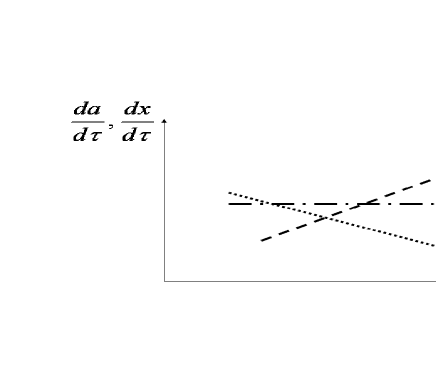
Figure 1: Phase diagram of a Robertson Walker universe. The dash and dot line corresponds to an inertial expansion (constant expansion rate); the dotted line is a decelerated expansion; the dashed line is an accelerated expansion. Observations tell us that the actual behaviour of the universe corresponds to both deceleration and acceleration, in different epochs. Relabelling the axes with an $x$ instead of $a$, and a $dx/dt$ instead of $da/d\tau$, the diagramme describes the state of a point particle interacting with a surrounding medium. Dash and dot is inertial motion (constant speed); dots is motion under the action of friction; dash is an accelerated motion driven by the medium.

Exactly the same type of phase space is obtained when describing the motion of a point particle interacting with a surrounding fluid. Now the interesting feature of this analogy is that we know how to write the equations governing the motion of a point particle of mass $m$ in a viscous fluid. Although dissipative, the problem can be treated starting from the Lagrangian

$$L=e^{\gamma t+\eta x}\frac{m}{2}\dot{x}^{2}\ .$$ (1)

A simpler form of this expression was initially introduced by Caldirola cald , then by others oth for different purposes. The Euler-Lagrange equation deduced from Eq. (1) is

$$\ddot{x}+\gamma\dot{x}+\dfrac{\eta}{2}\dot{x}^{2}=0\ ,$$ (2)

where $\gamma>0$ may be interpreted as the laminar viscosity coefficient and $\eta$ is the turbulent viscosity coefficient. Actually, Eq. (2) represents a viscous motion if for $\eta>0$ the motion is progressive; for regressive motion $\eta$ has to be assumed $<0$. In this approach, the properties of the fluid and of the interaction are all contained in $\gamma$ and $\eta$, that are assumed to be constants, which means that the fluid is not affected by the motion of the particle through it. Eq. (2) is however inadequate since it is not invariant for reversal of the $x$-axis. If $v_{0}$ is the initial velocity of the particle, the solution of (2) is

$$\dot{x}=\frac{2\gamma}{\left(\dfrac{2\gamma}{v_{0}}+\eta\right)e^{\gamma t}-\eta}\ ,$$ (3)

For $-\infty<v_{0}<-\frac{2\gamma}{\eta}$, the solution diverges at some finite positive time. We now recast the problem in a relativistic way. We shall consider a flat spacetime and introduce the action integral

$$S=-m\int_{A}^{B}e^{\alpha\tau^{\prime}-\beta x^{\prime}}ds\ ,$$ (4)

where $d\tau^{\prime}=cdt^{\prime}$, $v^{\prime}=\dot{x}^{\prime}$ and $ds=\sqrt{1-v^{\prime 2}/c^{2}}d\tau^{\prime}$. The exponent in Eq.(4) is assumed to be a true scalar, i.e. the scalar product of two four-vectors

$$\gamma = \left(\alpha,\beta,\beta,\beta\right)\ ,$$

$$r^{\prime} = \left(ct^{\prime},x^{\prime},0,0\right)\ .$$

The reference frame has been fixed so that the $x^{\prime}$ axis coincides with the direction of motion. Using Cartesian coordinates, the form of $\gamma$ expresses the expected space isotropy of the medium. The invariant associated with $\gamma$ is

$$\chi^{2}=\alpha^{2}-3\beta^{2}>0\ ,$$

and the four-vector has been assumed to be timelike. The Lorentz-invariant form of Eq. (4) is now

$$S=-m\int_{A}^{B}e^{\eta_{\alpha\beta}\gamma^{\alpha}x^{\beta}}ds\ ,$$ (5)

The Euler-Lagrange equation from (4) is

$$\ddot{x}^{\prime}-\frac{\beta}{2}c^{2}\left(1-\frac{\dot{x}^{\prime 2}}{c^{2}}\right)^{2}+\frac{\alpha}{c}\left(1-\frac{\dot{x}^{\prime 2}}{c^{2}}\right)\dot{x}^{\prime}=0\ .$$ (6)

Everything becomes more transparent and simpler if, applying an appropriate Lorentz transformation, we change the reference frame so that

$$\gamma=(\chi,0,0,0)\ .$$ (7)

We see that in this case a privileged reference frame exists: it is the one of the fluid (unprimed quantities). The equation of motion is now

$$\ddot{x}+\chi\left(1-\frac{\dot{x}^{2}}{c^{2}}\right)\frac{\dot{x}}{c}=0\ .$$ (8)

Equation(8) represents the relativistic version of motion in presence of laminar viscosity; now the solution is a decelerated motion and no troubles arise from any reversal of the space axes. It is explicitly:

$$\dot{x}=\pm\dfrac{v_{0}}{\sqrt{\dfrac{v_{0}^{2}}{c^{2}}+\left(1-\dfrac{v_{0}^{2}}{c^{2}}\right)e^{\frac{2\chi t}{c}}}}\ ,$$ (9)

Starting with an initial value $v_{0}<c,$ the velocity becomes zero in an infinite time; “photons” do not interact with the medium (their velocity stays equal to $c$). We could reasonably introduce a dependence of $\chi$ on $v$, but to discuss further this elementary situation is out of the scope of the present paper. What matters is that it is possible to give a Lagrangian treatment of a simple dissipative phenomenon describing a non-uniform evolution in time, in a relativistic context.

III The behaviour of spacetime

We may now use the model in the previous section as a guiding idea (by analogy) and the action (5) as a suggestion or inspiration to describe a spacetime that undergoes expansion or contraction at a non-uniform rate. We stress that not the whole universe but the only spacetime is considered.

The starting point is the usual Einstein-Hilbert action

$$S=\int_{\Omega_{1}}^{\Omega_{2}}Rd\Omega\ ,$$ (10)

where $R$ is the scalar curvature and $d\Omega=\sqrt{\left|g\right|}d^{4}x$ is the invariant volume element.

We directly introduce in the spacetime the kind of symmetry we usually attribute to the universe, i.e. four-dimensional isotropy around a given event. As it is well known the most general symmetric line element of this type is the RW one

$$ds^{2}=d\tau^{2}-a\left(\tau\right)^{2}\left[\frac{dr^{2}}{1-kr^{2}}+r^{2}\left(d\theta^{2}+\sin^{2}\theta d\phi^{2}\right)\right]\ ,$$ (11)

where $k=0$,$\pm 1$ and $r$ is a dimensionless coordinate (product of usual length times the square root of the space curvature). Introducing the metric tensor implicit in Eq. (11) into Eq. (10) one has

$$S=-6\mathcal{V}_{k}\int_{\tau_{1}}^{\tau_{2}}\left(a\ddot{a}+\dot{a}^{2}+k\right)ad\tau\ ,$$ (12)

where $\mathcal{V}_{k}=\int_{0}^{r}\int_{0}^{\pi}\int_{0}^{2\pi}\frac{r^{2}\sin\theta}{\sqrt{1-kr^{2}}}drd\theta d\phi$ and dots represent derivatives with respect to $\tau$.

III.1 “Dissipative” spacetime

To take advantage of the simple example described in Sec. II, we may want to reproduce the same logical structure while building the action integral. Of course, there are important differences to take into account. In Sec. II we had two “actors” entering the scene, the particle and the dissipative medium, and an interaction between them. The interaction was mediated by a four-vector pertaining to the medium and another one describing the state (of motion) of the particle. Now the “actor” is unique, spacetime itself, and nothing is moving across it. However, we may think to the motion of the representative point of the state of a hypersurface labelled by $\dot{a}$ in a bidimensional phase space where the independent variable is the parameter $a$. Again, we associate to the system a four-vector $\gamma$ which couples to the state variable in the same way as in the simple expression (5). There the position coordinate of the particle appeared in the Lagrangian through its (first) derivative $dx/dt$; now, the Lagrangian is written in terms of the (second) derivatives of the elements of the metric tensor. The simplest way to couple a vector to the metric in order to generate a scalar is by taking the norm of the vector itself, so we are led to conjecture the following action integral

$$S=\int_{\Omega_{1}}^{\Omega_{2}}e^{\pm g_{\mu\nu}\gamma^{\mu}\gamma^{\nu}}Rd\Omega\ ,$$ (13)

where $\gamma$ is meant to represent an internal property of spacetime. The correspondence between (13) and (5) may be better seen considering that in (5) the position vector of the particle is made out of the coordinates of the particle, whose choice is free, and the final behaviour of the system is independent from that choice. In the case of (13), i.e. for spacetime, the "coordinates" used to describe the state of the system are represented by the elements of the metric tensor and again there is a gauge freedom in their choice. As written above, the simplest scalar we can build from a vector and the metric tensor is the one in the exponent of (13).

Using the metric in the form (11), in the (privileged) cosmic reference frame, and the four-dimensional rotation symmetry, $\gamma$ necessarily appears in the “radial” form of Eq. (7), so that the action (13) reads

$$S=-6\mathcal{V}_{k}\int_{\tau_{{}_{1}}}^{\tau_{{}_{2}}}e^{\pm\chi^{2}}\left(a\ddot{a}+\dot{a}^{2}+k\right)ad\tau\ .$$ (14)

The $\chi$ = constant case is irrelevant because it corresponds to simple Minkowski spacetime (the exponential may be absorbed in a rescaling of the time coordinate). Non-trivial solutions exist only if

$$\chi\equiv\chi\left(a\left(\tau\right)\right)\ ,$$ (15)

and spacetime is not globally homogeneous and isotropic. The observation of the universe apparently tells us that space is flat, so we further assume $k=0$. The final effective Lagrangian is

$$\mathcal{L=}e^{\pm\chi^{2}}\left(a\ddot{a}+\dot{a}^{2}\right)a\ .$$ (16)

The Euler-Lagrange equation for $a\left(\tau\right)$ is

$$\frac{d^{2}}{d\tau^{2}}\left(\frac{\partial\mathcal{L}}{\partial\ddot{a}}\right)-\frac{d}{d\tau}\left(\frac{\partial\mathcal{L}}{\partial\dot{a}}\right)+\frac{\partial\mathcal{L}}{\partial a}=0\ ,$$ (17)

or explicitly

$$\ddot{a}\left(1\pm 2\chi\chi^{\prime}a\right)$$ (18)

$$+\dfrac{\dot{a}^{2}}{a}\left\{a^{2}\left(2\chi^{2}\chi^{\prime 2}\pm\chi^{\prime 2}\pm\chi\chi^{\prime\prime}\right)\pm 3a\chi\chi^{\prime}+\dfrac{1}{2}\right\}=0\ .$$

where $\chi^{\prime}\equiv d\chi/da$. A trivial and non interesting solution is obtained for $a=\mathrm{constant}$ (Minkowski spacetime). Other solutions however exist. The above equation may be reorganized in the form

$$\dfrac{\ddot{a}}{\dot{a}}=-f(a)\dot{a}\ ,$$ (19)

where

$$f(a)=\dfrac{2a^{2}\left(2\chi^{2}\chi^{\prime 2}\pm\chi^{\prime 2}\pm\chi\chi^{\prime\prime}\right)\pm 6a\chi\chi^{\prime}+1}{2a\left(1\pm 2a\chi\chi^{\prime}\right)}\ .$$ (20)

A first integration leads to

$$\dot{a}=Ae^{-\int^{a}f\left(\zeta\right)d\zeta}\ ,$$ (21)

and finally to

$$\tau=\frac{1}{A}\int_{0}^{a}e^{\int^{\varsigma}f\left(\zeta\right)d\zeta}d\varsigma\ .$$ (22)

III.2 Choosing $\chi\left(a\right)$

The function $\chi(a)$ in our case is something which is “given” exactly as the global symmetry is. We shall discuss this issue in more detail in the next section. What matters here is that $\chi(a)$ is not deducible from a variational principle. Should we try and write its field equation from the action of Eq. (14), the result would trivially be $\chi=0$, i.e. empty and flat spacetime. A singularity, as well as a symmetry, is here an initial condition and not a consequence of something else. This means that we need criteria and guesses to think about credible forms for $\chi(a)$, consistent with the hypotheses. One reasonably simple criterion for a vector field that is expected not to spoil the symmetry we assumed for spacetime, is to constrain it to be divergence free everywhere except in the center of symmetry/origin of the cosmic times. In fact, any event where the divergence of the vector differs from zero may be thought of as a “source” and, since we need to preserve homogeneity and isotropy, we would have to assume a continuous and uniformly distributed source. Being, in this paradigm, $\gamma$ a concrete quantity strictly related to the presence of a singularity, it seems more reasonable to have just one pointlike source in the origin. There is however also a different, though somehow equivalent, reason for choosing $\gamma$ to be divergenceless, as we shall see further on (Sec. III.3 ), when considering the analogy with a defected solid.

The null–divergence condition is formally written as

$$0=\gamma_{\;\;;\mu}^{\mu}=\left(\sqrt{\left|g\right|}\gamma^{\mu}\right)_{,\mu}\ ,$$ (23)

where the semicolon represents a covariant derivative. The solution of this equation is

$$\chi=\frac{Q^{3}}{a^{3}}\ .$$ (24)

In practice, the vector field looks like the “electric” field of a point charge $Q^{3}$, but in four dimensions. Inserting this result in Eq. (19), and expressing $a$ in units of $Q$, we obtain

$$\frac{\ddot{a}}{\dot{a}}=-\dfrac{36\pm 24a^{6}+a^{12}}{2a^{7}(a^{6}\mp 6)}\dot{a}\ .$$ (25)

As a consequence, we have

$$\dot{a}=\sqrt{\dfrac{a^{5}}{a^{6}\mp 6}\;\,e^{\mp 1/a^{6}}}\ .$$ (26)

Choosing the upper signs in (26), as well as in (14), the expansion rate acquires real values starting from a finite non-zero value of $a$, then it displays a monotonic trend which does not correspond to observational data. Choosing the lower signs instead, we see that the expansion rate $\dot{a}$ has two extrema at

$$a_{M\pm}=\sqrt[3]{3\pm\sqrt{3}}\ .$$ (27)

The corresponding explicit numeric values for the scale factors are

$$a_{M_{-}} = 1.08\ ,$$ (28)

$$a_{M_{+}} = 1.68\ .$$ (29)

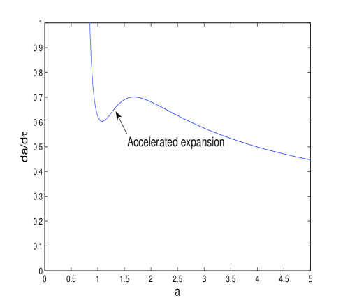
Figure 2: Plot of $da/d\tau$ as a function of $a$, in empty spacetime. Two extrema delimiting a phase of accelerated expansion are clearly seen.

Fig. 2 shows the behaviour of $da/d\tau$ as a function of the scale factor $a$. In any case, the asymptotic behaviour when $a\rightarrow\infty$ is $\dot{a}\rightarrow 0$: this is a never-ending expansion. From now on, we limit our consideration to the latter choice of signs, so, integrating Eq. (26) one has

$$\tau=\int_{0}^{a}\frac{\left(\zeta^{6}+6\right)^{1/2}}{\zeta^{5/2}}e^{-1/2\zeta^{6}}d\zeta\ .$$ (30)

The corresponding behaviour of the scale parameter $a$ as a function of the cosmic time $\tau$ is shown in Fig. 3.

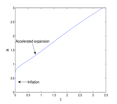
Figure 3: Scale factor $a$ as a function of cosmic time $\tau$; arbitrary units. The initial inflationary epoch as well as an accelerated expansion between $\tau\simeq 0.41$ and $\tau\simeq 1.3$ are clearly visible.

Close to the origin the negative exponential factor in the integral in (30) brings about an inflationary phase, that cannot be resolved in Fig. 3, followed by a deceleration-acceleration-deceleration sequence driving an unlimited expansion. In the neighborhood of the origin the scale factor $a$ does indeed grow faster than any power of $\tau$.

We can now fix the scale of the expansion. We know that in general

$$\frac{a_{0}}{a}=1+z\ ,$$ (31)

where $a_{0}$ is the present value of the scale factor and $z$ is the redshift of light emitted when the scale factor was $a$. From the numerical values (28) and (29) we see that the ratio between the scale factor at the end and at the beginning of the acceleration epoch is

$$\frac{a_{M+}}{a_{M-}}=1.55\ .$$ (32)

Then, using (31), we can fix

$$\frac{1+z_{i}}{1+z_{f}}=1.55\ ,$$ (33)

where now $z_{i}$ corresponds to the redshift at $a_{M-}$ and $z_{f}$ to that at $a_{M+}$. Looking at the data from the observation of high redshift Ia supernovae  perlmutter , we see that (33) is indeed consistent with an initial value of $z_{i}\sim$ $1.6$ (or a little more) and a final one $z_{f}\sim 0.6$. This result is obtained independently from the value of the integration constant $Q$ and in the absence of matter.

An estimate of $Q$ can be obtained again from (31). If we let the $a_{M-}$ value correspond to $z_{i}=1.6$, we get immediately, from (31) and (28), $a_{0}=2.81$, then numerically from (30) $\tau_{0}=3.06$. Now, if $T$ is the age of the universe, it is

$$\tau_{0}=\frac{cT}{Q}\ .$$ (34)

If we constrain $T$ to be not less than 12 billion years (age of the oldest globular cluster stars), we conclude that

$$Q\gtrsim 4\times 10^{25}\quad\mathrm{m}\ .$$ (35)

This result should also be confirmed considering the present value of the Hubble constant $H_{0}$. From (26) (lower signs) we see that

$$\tilde{H}_{0}=\left.\frac{\dot{a}}{a}\right|_{\tau=\tau_{0}}=\frac{a_{0}^{3/2}}{\left(a_{0}^{6}+6\right)^{1/2}}e^{1/(2a_{0}^{6})}=0.21\ .$$ (36)

The above result is adimensional. Introducing the appropriate dimensions it must be

$$H_{0}=\tilde{H}_{0}\frac{c}{Q}=1.6\times 10^{-18}\text{ s}^{-1}$$ (37)

or, using the commonly used units,

$$H_{0}\simeq 49\text{ km/s}\times\text{Mpc,}$$ (38)

Considering the roughness of the model, this is a reasonable number for the Hubble constant, which is currently estimated to be $65$ km/s$\times$Mpc  conley .

We would like to stress that all this comes from an internal property of spacetime, with no matter inside. Matter must be further added to the Lagrangian in the traditional (additive) way and with a minimal coupling to spacetime via the metric tensor.

III.3 What could the vector field represent?

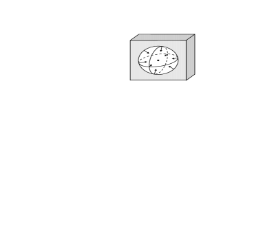
Figure 4: Point defect originated removing a solid hypersphere, then squeezing the hole to a point.

As mentioned above, the "internal" vector field associated with empty spacetime can be interpreted by means of another analogy with ordinary physics. We know that the intrinsic metric of a material continuum can be non-Euclidean (non-zero intrinsic curvature) when defects are present (see for example  eshelby or  kat and references therein). The corresponding theory has been developed many years ago, starting with the formal definition of a defect given by V. Volterra volterra . The attempt to extend the theory from material elastic media to spacetime has been made by many a scientist Kleinert ; atarta ; katanaev ; malyshev ; difetti ; padmana in various epochs, without leading to a complete formal new theory. The similarities are indeed tempting. What is easily seen is that, whenever a portion of a continuum is removed (or more is added) each point in the material is displaced to a new position (in the unperturbed original reference frame) miofriedman

$$x^{i\prime}=x^{i}+\xi^{i}\ .$$ (39)

The new coordinates are obtained by means of a vector displacement field $\xi_{i}$. In the continuum a new metric is now induced, which is not the original Euclidean one $\delta^{ij}$, but

$$g^{ij}=\delta^{ij}+2\varepsilon^{ij}\ ,$$ (40)

where

$$\varepsilon_{ij}=\frac{1}{2}\left(\frac{\partial\xi_{i}}{\partial x^{j}}+\frac{\partial\xi_{j}}{\partial x^{i}}+\delta^{lm}\frac{\partial\xi_{l}}{\partial x^{i}}\frac{\partial\xi_{m}}{\partial x^{j}}\right)\ ,$$ (41)

is the (non-linear) strain tensor. It is important to remark that the new metric, as well as all physical quantities of this description, can equally well be expressed in terms of the original, undeformed "Lagrangian" coordinates $x_{i}$, or of the new intrinsic coordinates $x_{i}^{\prime}$, being the old and the new coordinates numerically identified  eshelby . In both cases any point is labelled by the same set of numbers (the coordinates) plus a vector (the displacement vector at that point) which is actually zero in the unstrained manifold and non-zero in the strained one.

This framework can be generalized to four dimensions and to spacetime. The Euclidean basic metric  $\delta_{ij}$ is then replaced by the one of Minkowski $\eta_{\mu\nu}$ and the induced metric is written as miofriedman :

$$g_{\mu\nu}=\eta_{\mu\nu}+2\varepsilon_{\mu\nu}\ .$$ (42)

Without further details, let us consider an unperturbed (i.e., Euclidean) $4$-dimensional space. Then, let us suppose we remove a $4$-sphere and close the hollow by pulling radially on each point of the hypersurface of the hole. The situation is described in Fig. 4. This procedure induces a radial displacement field represented by a radial four-vector $\xi$. Remarkably, solving the equations of the elasticity theory with these symmetry conditions gives, for $\xi$ in four dimensions, precisely a result like Eq. (24): the four-vector $\xi$ has a null divergence (see for instance Ref. eshelby , Vol. 3 page 107). For spacetime, which implies a Wick rotation in order to produce the right signature, the induced interval we obtain in these conditions, once expressed in appropriate coordinates, corresponds to a typical Robertson-Walker metric

$$ds^{2}=d\tau^{2}-a^{2}\left(\tau\right)\left[d\psi^{2}+\psi^{2}\left(d\theta^{2}+\sin^{2}\theta d\phi^{2}\right)\right]\ ,$$ (43)

where $a\left(\tau\right)$ is a non-trivial function and space is flat. In order to better explain this result, let us start from the general form of the line element of a Minkowski spacetime expressed in four dimensional polar coordinates

$$ds^{2}=da^{2}-a^{2}\left[d\psi^{2}+\psi^{2}\left(d\theta^{2}+\sin^{2}\theta d\phi^{2}\right)\right]\ ,$$ (44)

where $a$ is now the radial coordinate. The point defect produces, as written above, a purely radial displacement field, which means that the only non-vanishing element of the strain tensor (41) is $\varepsilon_{aa}$. The induced metric, according to (42), is then

$$ds^{2}=\left(1+\frac{\partial\xi_{a}}{\partial a}\right)^{2}da^{2}-a^{2}\left[d\psi^{2}+\psi^{2}\left(d\theta^{2}+\sin^{2}\theta d\phi^{2}\right)\right]$$ (45)

Redefining the radial (actually time) coordinate so that

$$d\tau=\left(1+\frac{\partial\xi_{a}}{\partial a}\right)da\ ,$$ (46)

the old radial coordinate $a$ is expressed as a function of the new time and the line element becomes (43), as claimed.

In order to clarify the meaning of the $\gamma$ vector, we apply a procedure typical of the elasticity theory. In a deformed medium the strain is of course accompanied by a stress. In linear theory, which we now consider for simplicity, the stress tensor $\sigma_{\mu\nu}$ depends linearly on the strain tensor $\varepsilon_{\mu\nu}$ (Hooke’s law). In our case the chosen symmetry implies that the radial-radial components of both tensors (i. e. $\sigma_{aa}$ and $\varepsilon_{aa}$) be proportional to each other. The next step is to think of a given solid angle centered at the singularity, then isolate a portion of it delimited by two transverse (orthogonal to the radius) (hyper)surfaces. In an equilibrium state the forces on opposite faces of the boundary of the envisaged piece of material must be equal in strength. By definition the components of the force on a small surface (four-dimensional space) are

$$f^{\mu}=\frac{1}{3!}\sigma^{\mu\nu}\epsilon_{\nu\alpha\beta\lambda}dx^{\alpha}\wedge dx^{\beta}\wedge dx^{\lambda}\ .$$ (47)

Calling again in the symmetry, we see that on the “bases” of our portion of solid angle (47) becomes

$$f^{a}=\mathcal{K}\varepsilon^{aa}a^{3}d\theta d\phi d\psi\ ,$$ (48)

where $\mathcal{K}$ is a constant and $\theta$, $\phi$, $\psi$ are angles. Now we see that the equilibrium within a given solid angle implies that $f^{a}$ be independent from $a$ ; in practice it must be

$$\varepsilon^{aa}a^{3}=\text{ constant}\ .$$ (49)

Eq. (49) is in fact a conservation law. Introducing the four-vector

$$\gamma=\varepsilon\cdot n\ ,$$ (50)

where $n$ is a unit vector orthogonal to a given surface and $\gamma$ represents the flux density of strain. We see that the flux of $\gamma$ across any closed surface is zero, i.e. $\nabla\cdot\gamma=0$. Let us identify the $\gamma$ in (50) with the old one, so its radial component (the only non-zero component, in our case) will be, as before and now by virtue of (49) and (50),

$$\chi=\frac{Q^{3}}{a^{3}}\ .$$

The extended elasticity theory helps us also to find a meaning to the $Q$ constant. We know that the energy needed to close a void is given by the product of the pressure times the squeezed volume $W=pV$. In our case, with the help of the pictorial view of the situation shown on Fig. 4, we see that the equivalent of the “energy” is proportional to

$$\varepsilon_{aa}\mathcal{A}^{4}\ ,$$

where $\mathcal{A}$ is the radius of the initial hollow. Calling in (49) and (50) we see that the "energy" is proportional to $Q^{3}\mathcal{A}$. $Q^{3}$ is a measure of the ratio between the work done to create the defect and its radius.

This is a consistent logical framework. Part of it relies on geometrical bases, whose meaning is clear in spacetime as well as in three dimensions; this is the case of the strain tensor and of the definition  (50) for $\gamma$. The rest, i.e. the stress tensor with the related quantities, is intuitively clear in three dimensions, much less in four, however it is a tool for arriving to the final interpretation, which remains essentially geometrical.

III.4 Equivalent matter distribution

Once the metric tensor is defined, we can compute from it the Einstein tensor and, taking the Einstein equations literally, interpret it as being proportional to the energy-momentum tensor of some matter-energy distribution responsible for the peculiar metric. Doing this exercise in our case produces the following effective energy-momentum tensor:

$$T_{\tau}^{\tau} = \frac{G_{\tau}^{\tau}}{\kappa}=\frac{3}{\kappa}\left(\frac{\dot{a}}{a}\right)^{2}=\frac{3}{\kappa Q^{2}}\frac{a^{3}}{a^{6}+6}e^{1/a^{6}}\ ,$$ (51)

$$T_{r}^{r} = \frac{G_{r}^{r}}{\kappa}=\frac{2a\overset{\cdot\cdot}{a}+\dot{a}^{2}}{\kappa a^{2}}=\frac{6}{\kappa Q^{2}}\frac{(5a^{6}-6)}{a^{3}\left(a^{6}+6\right)^{2}}e^{1/a^{6}}\ ,$$ (52)

$$T_{\theta}^{\theta} = T_{\phi}^{\phi}=T_{r}^{r}\ ,$$ (53)

where it is $\kappa=8\pi G/c^{4}$.

This energy-momentum tensor has the appearance of the one of a perfect fluid whose effective matter-energy density is

$$\rho=\frac{3}{\kappa Q^{2}}\frac{a^{3}}{a^{6}+6}e^{1/a^{6}}\ .$$ (54)

The corresponding effective pressure is

$$p=\frac{6}{\kappa Q^{2}}\frac{5a^{6}-6}{a^{3}\left(a^{6}+6\right)^{2}}e^{1/a^{6}}\ ,$$ (55)

and is represented in Fig. 5. The initially negative values correspond to inflation.

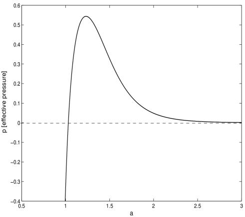
Figure 5: Effective pressure as a function of the scale parameter $a$. Arbitrary units. The initial negative values correspond to an inflationary epoch.

From Eqs. (54) and (55) one can immediately obtain the Equation of State (EOS) of this fluid

$$p=\frac{2(5a^{6}-6)}{a^{6}(a^{6}+6)}\rho\ .$$ (56)

The pressure stays negative up to $a^{6}=6/5$. In the language of dark energy theories this is equivalent to a peculiar choice of the factor $w=p/\rho$. Of course in the case of those theories the equation of state (56) would come from a different Lagrangian than ours; however here the comparison is done only at the final stage. What we would like to stress is that such an equation of state, if sought directly, would appear to be rather artificial and indeed it is, if thought as pertaining to an actual "fluid" of any sort.

IV The effect of matter

Let us now verify what the effect of matter is in a spacetime like the one described before. To this aim, we consider the conceptually simplest situation and introduce a perfect fluid minimally coupled to the geometry, so that the total Lagrangian of the problem is (see Ref. Schutz and references therein)

$$S=\int_{\Omega_{1}}^{\Omega_{2}}e^{-g_{\mu\nu}\gamma^{\mu}\gamma^{\nu}}Rd\Omega+\kappa\int_{\Omega_{1}}^{\Omega_{2}}pd\Omega\ ,$$ (57)

where $p$ is the pressure of the matter-energy fluid. Following the traditional approach, we consider that in the present time the fluid is reduced to an almost incoherent dust, i. e. $p\simeq 0$. In this condition and with the RW symmetry the matter energy density scales as $\rho=\rho_{0}/a^{3}$ (matter conservation) so that its contribution to the Lagrangian is simply a constant: the expansion law is unaffected. When the presence of the fluid is relevant is in the early epochs where the matter density is assumed to be negligible with respect to the pressure (radiation dominated universe). Conservation of entropy together with matter brings about a pressure that scales as $a^{-4}$

$$p=\frac{\psi}{\kappa a^{4}}\ ,$$ (58)

where $\psi$ is a positive parameter and $\kappa$ has been included for convenience. From (57) and in the case of the RW symmetry, we obtain the Euler-Lagrange equation:

$$2\left(a+\frac{6}{a^{5}}\right)\ddot{a}+\left(\frac{36}{a^{12}}+1-\frac{24}{a^{6}}\right)\dot{a}^{2}-\frac{\psi}{a^{2}}e^{1/a^{6}}=0\ .$$ (59)

Condition (23) has again been imposed on the 4-vector $\gamma$, as before, so that (24) holds.

Looking for solutions that, in the absence of matter, reduce to the already known case (26) we pose

$$\dot{a}=f\left(a\right)e^{\lambda/a^{6}}.$$ (60)

Here $f(a)$ is a function of the expansion parameter $a$, and $\lambda$ is a constant to be determined later. Differentiating Eq. (60) with respect to cosmic time $\tau$ gives

$$\ddot{a}=f\left(f^{\prime}-6f\frac{\lambda}{a^{7}}\right)e^{2\lambda/a^{6}}\ .$$ (61)

where $f^{\prime}\equiv df/da$.

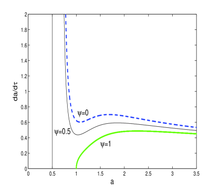
Figure 6: Behaviour of the expansion rate of the universe in the presence of ordinary matter: the solid line shows the dependence of $a$ on the cosmic time in the case of a spacetime with matter in subcritical conditions with $\psi=0.5$. For the sake of comparison we also show the empty spacetime case ($\psi=0$, dashed line) and a case of supercritical matter density ($\psi=1$, thick grey line). We note that the three curves start with an accelerated expansion phase. For later times this is converted into deceleration, but for $\psi=0.5$ and $\psi=0$ an effective “re-heating” occurs.

Introducing Eqs. (61) and (60) into Eq. (59) gives

$$2\left(a+\frac{6}{a^{5}}\right)ff^{\prime}e^{2\lambda/a^{6}}$$ (62)

$$+\left(1+\frac{36-72\lambda}{a^{12}}-\frac{24+12\lambda}{a^{6}}\right)f^{2}e^{2\lambda/a^{6}}-\frac{\psi}{a^{2}}e^{1/a^{6}}=0\ .$$

Choosing $\lambda=1/2$, this equation becomes

$$2ff^{\prime}\left(a+\frac{6}{a^{5}}\right)+f^{2}\left(1-\frac{30}{a^{6}}\right)-\frac{\psi}{a^{2}}=0\ .$$ (63)

The solution of (63) is

$$f^{2}=\frac{Aa^{5}-\psi a^{4}}{6+a^{6}}\ ,$$ (64)

$A$ is an integration constant.

Finally (60) tells us that the expansion rate is:

$$\dot{a}=a^{2}\left(\frac{a-\psi}{6+a^{6}}\right)^{1/2}\exp\left(\frac{1}{2a^{6}}\right).$$ (65)

A comparison with (26) fixes $A=1$ and the overall sign of the formula.

From (65) we see that the model fails to describe the situation for

$$0\leq a<\psi$$ (66)

(imaginary expansion rate). At a smaller scale evidently some more refined picture is needed.

Looking for the extrema and differentiating (65) one obtains the condition:

$$a\left(a^{12}-24a^{6}+36\right)+2\psi\left(9a^{6}-18-a^{12}\right)=0\ .$$ (67)

For $\psi=0$ the solutions of (67) are (27). Studying the equation for $\psi>0$ we see that three real positive roots exist as far as $0<\psi<\psi_{c}$, where $\psi_{c}\simeq 0.8$; this means that $\dot{a}$ has three extrema. For $\psi>\psi_{c}$ only one extremum exists. Fig. (6) compares the behaviours of an empty spacetime with those of one with, respectively, a sub- and a super-critical matter content.

In practice, when matter is present in the form of a radiation fluid, the model starts working from a typical value $a=\psi$ of the scale factor. Initially one has a phase of inflationary accelerated expansion, then the expansion rate starts decreasing, but after a while, if it is $\psi$ smaller than the critical value, a sort of re-heating happens and the universe accelerates again its expansion; finally the expansion rate decreases once more until reaching the $0$ value at infinity. When $\psi>\psi_{c}$ the initial accelerated expansion is followed by a never ending deceleration.

The parameter $\psi$ scales as $Q^{2}$, thus, using the estimate of Eq. (35), we see that the critical value, in international units, is

$$\psi_{c}\sim 10^{50}\text{ m}^{2}\ .$$ (68)

Should we conjecture that the minimal $a_{P}$ value, below which the classical fluid description fails, is the Planck length, it would be

$$\psi_{P}\sim 10^{-10}\text{ m}^{2}\ .$$ (69)

Actually one has that (see for instance  MTW )

$$\psi=\frac{\kappa}{3}\rho_{r_{0}}a_{0}^{4}\ ,$$ (70)

where $\rho_{r_{0}}$ is the present radiation energy density in the universe and $a_{0}$ its present scale factor. One usually estimates that $\rho_{r_{0}}\sim$ $10^{-13}$ J/m³; using for $a_{0}$ the order of magnitude of $Q$ we obtain

$$\psi\sim 10^{38}\text{ m}^{2}\ ,$$ (71)

or, in the adimensional form used throughout the paper, $\psi\sim 10^{-10}$, well inside the subcritical region. The corresponding minimal scale of the universe (below which the model is not able to describe what happens) would be

$$a_{m}\sim 10^{13}\mathrm{m}.$$ (72)

The conclusion of this section is that the presence of ordinary matter apparently does not spoil the results obtained in Sec. III for empty spacetime.

V The Newtonian limit

Of course our theory, as any cosmological theory, must prove to be able to reproduce the known results at the scale of the Solar system and weak gravitational field, which means that it should possess a Newtonian limit.

In order to prove this it is convenient to start from the action integral (57) and write the general form of the Euler-Lagrange equations of the theory:

$$e^{-g_{\alpha\beta}\gamma^{\alpha}\gamma^{\beta}}\left(G_{\mu\nu}-\gamma_{\mu}\gamma_{\nu}R\right)$$

$$+g_{\mu\nu}e^{-g_{\alpha\beta}\gamma^{\alpha}\gamma^{\beta}}\left(2\gamma^{\alpha}\gamma_{\alpha;\sigma}\gamma_{\lambda}\gamma^{\lambda;\sigma}-\gamma^{\alpha;\sigma}\gamma_{\alpha;\sigma}-\gamma^{\alpha}\gamma_{\alpha;\sigma}^{;\sigma}\right)$$

$$-\frac{1}{2}e^{-g_{\alpha\beta}\gamma^{\alpha}\gamma^{\beta}}g_{\sigma\nu}\left(2\gamma^{\alpha}\gamma_{\alpha;\mu}\gamma_{\lambda}\gamma^{\lambda;\sigma}-\gamma^{\alpha;\sigma}\gamma_{\alpha;\mu}-\gamma^{\alpha}\gamma_{\alpha;\mu}{}^{;\sigma}\right)$$ (73)

$$-\frac{1}{2}e^{-g_{\alpha\beta}\gamma^{\alpha}\gamma^{\beta}}g_{\sigma\mu}\left[\mu\rightarrow\nu\right]$$

$$=\kappa\mathsf{T}_{\mu\nu}.$$

The terms on the second and third line are symmetrized in $\mu$ and $\nu$ and $\mathsf{T}_{\mu\nu}$ is the energy-momentum tensor of matter.

Now suppose that

$$\mathsf{T}_{\mu\nu}=\mathcal{T}_{\mu\nu}+T_{\mu\nu}$$

where $\mathcal{T}_{\mu\nu}$ is the energy momentum tensor of the cosmic fluid and $T_{\mu\nu}$ is the one of a bunch of matter, we assume for simplicity to have stationary space isotropy around any given point.

Under these conditions we expect the perturbed line element (spacely isotropic coordinates) to be:

$$ds^{2}=\left(1+h_{0}\right)d\tau^{2}-a^{2}\left(1+h_{s}\right)\left(dx^{2}+dy^{2}+dz^{2}\right)$$ (74)

with $h_{0}$, $h_{s}<<1$ and depending on $r=\sqrt{x^{2}+y^{2}+z^{2}}$ only.

The perturbed metric tensor will perturb the flow lines of the vector $\gamma$ field also, inducing the same kind of space symmetry. So we write for the components of the perturbed vector:

$$\Upsilon^{0} = \chi\left(1+f_{0}\right)$$ (75)

$$\Upsilon^{i} = \chi f_{s}\frac{x^{i}}{r}$$

where the $f$’s are assumed to depend on $r$ only (as the $h$’s from which they stem) and $f_{0}$, $f_{s}<<1$ (at least as small as $h$’s).

Recalling that the $\Upsilon$ field has its origin in the cosmic point defect and that no other defect has been introduced, the divergencelessness condition $\Upsilon_{;\mu}^{\mu}=0$ must still hold. Using the equivalent form $\left(\sqrt{-\mathsf{g}}\Upsilon^{\mu}\right)_{,\mu}=0$, the zero order (unperturbed) solution $\chi=1/a^{3}$, (74), and the dependences of the $f$’s and $h$’s, we obtain in the first order approximation

$$\left(f_{s}\frac{x^{i}}{r}\right)_{,i}=0$$ (76)

which implies

$$f_{s}=\frac{b}{r^{2}}$$ (77)

$b$ is an integration constant.

A further constraint we can introduce is that the norm of the $\Upsilon$ vector remains unchanged. This is because, again, the vector field depends solely on the existence of a defect and the global symmetry it induces. Considering this constraint we write

$$\Upsilon_{\mu}\Upsilon^{\mu}=\gamma_{\mu}\gamma^{\mu}=\chi^{2}$$

or, using (74), (75), and stopping at the first order,

$$\chi^{2}=\chi^{2}\left(1+2f_{0}+h_{0}\right)$$

which implies

$$f_{0}=-\frac{h_{0}}{2}$$ (78)

Once these constraints have been implemented we may go back to (73) and consider the time-time equation:

$$e^{-\chi^{2}}\left(G_{00}-\gamma_{0}^{2}R\right)\\ +g_{00}e^{-\chi^{2}}\left(2\gamma^{\alpha}\gamma_{\alpha;\sigma}\gamma_{\lambda}\gamma^{\lambda;\sigma}-\gamma^{\alpha;\sigma}\gamma_{\alpha;\sigma}-\gamma^{\alpha}\gamma_{\alpha;\sigma}^{;\sigma}\right)\\ -e^{-\chi^{2}}g_{\sigma 0}\left(2\gamma^{\alpha}\gamma_{\alpha;0}\gamma_{\lambda}\gamma^{\lambda;\sigma}-\gamma^{\alpha;\sigma}\gamma_{\alpha;0}-\gamma^{\alpha}\gamma_{\alpha;0}{}^{;\sigma}\right)\\ =\kappa\mathsf{T}_{00}.$$

The metric tensor is diagonal, which fact implies

$$e^{-\chi^{2}}\left(G_{00}-\gamma_{0}^{2}R\right)\\ +g_{00}e^{-\chi^{2}}\left(2\gamma^{\alpha}\gamma_{\alpha;i}\gamma_{\lambda}\gamma^{\lambda;i}-\gamma^{\alpha;i}\gamma_{\alpha;i}-\gamma^{\alpha}\gamma_{\alpha;i}^{;i}\right)\\ =\kappa\mathsf{T}_{00}.$$

The next step is to expand everything up to the first order in $h$’s and $f$’s; drop the zero order terms, which are satisfied by (24) and (65) with the source $\mathcal{T}_{00}$; use conditions (78) and (76). The remaining first order equation is:

$$-3\frac{\dot{a}^{2}}{a^{2}}h_{0}$$

$$+\frac{1}{a^{2}}\left(h_{s,xx}+h_{s,yy}+h_{s,zz}\right)$$

$$+\frac{\chi^{2}}{a^{2}}\left(h_{0,xx}+h_{0,yy}+\allowbreak h_{0,zz}\right)$$ (79)

$$+2\frac{\chi^{2}}{a^{2}}\left(h_{s,xx}+h_{s,yy}+h_{s,zz}\right)$$

$$=\kappa e^{\chi^{2}}T_{00}$$

Now, for ordinary time scales the rate of change of $a$, i.e. the Hubble constant, is extremely small so that we neglect the first term in (79). Passing to an orthonormal base (marked by a $\sim$) the factors $1/a^{2}$ are absorbed into the space derivatives, so that (79) becomes:

$$\tilde{\nabla}^{2}h_{s}+\chi^{2}\left(\tilde{\nabla}^{2}h_{0}+2\tilde{\nabla}^{2}h_{s}\right)=\kappa e^{\chi^{2}}T_{00}$$ (80)

Finally, exploiting the gauge freedom in the choice of the coordinates (Lorentz gauge with time independent $h$’s), (80) is reduced to

$$\tilde{\nabla}^{2}\bar{h}_{0}=-\kappa\frac{e^{\chi^{2}}}{1+\chi^{2}}T_{00}$$

which can be read as the Poisson equation for a Newtonian gravitational potential with a renormalized coupling constant

$$\kappa^{\ast}=\kappa\frac{e^{\chi^{2}}}{1+\chi^{2}}$$

slowly changing in cosmic times. The vector field $\gamma$ appeares at the local scale only through its norm $\chi^{2}$ included in the renormalization factor of the Newton gravitational constant $G$.

VI Conclusion and discussion

We have applied a heuristic approach to the problem of describing the behaviour of the universe in its expansion. Instead of introducing new components in what should correctly be called “matter” (any scalar or tensor field usually considered is indeed “matter” in the sense that it contributes to the right hand side of the Einstein equations and appears additively in the Lagrangian), we have used a model based on the idea that the very spacetime is endowed with a property analogous to the internal viscosity of a fluid. This feature has been treated introducing an exponential factor in the Langrangian and exploiting from the very beginning the four-symmetry we think the universe has around the origin. The scalar in the exponent of the new factor is thus built from a radial (in four dimensions) vector field. Symmetry considerations suggest that the vector field can be divergenceless everywhere except in the origin. Solving the vacuum Einstein equations in these conditions we end up with a global RW metric with a scale factor depending on cosmic time in such a way to reproduce an initial inflationary era, followed by a decelerated, then again accelerated, and finally decelerated expansion of the universe, or, to say better, of space itself.

Looking for a possible explanation of the “friction” described by the new vector field, we have had recourse to a further analogy with ordinary material continua. We have assimilated empty spacetime to a four-dimensional continuum containing a pointlike defect, and then we have analyzed the strain and consequent metric tensor induced by such a defect. The final result is again a RW metric with a time dependent scale factor. The radial displacement field of this scenario is divergence-free as the strain flux density is, thus allowing the identification of the latter with the initial “viscous” vector field. The model described here presents results that scale as the“strength” or “charge” of the center of symmetry, which may be fixed in order to reproduce the expected age of the universe; this parameter is geometrically interpreted as representing both the size of the original void and the “rigidity” of spacetime, where the final defect (initial singularity) comes from. Besides this fact, the model, without any further recourse to free parameters, reproduces reasonably well the observed duration of the acceleration era. Furthermore, it gives also rise to an initial inflationary era.

One can wonder what changes this theory brings about in the Newtonian limit and on a local scale. It is easy to see that with respect to this nothing happens. The relevant quantity in the action (14) is the scalar $\chi^{2}$ whose rate of change with cosmic time is $2\dot{\chi}/\chi=-6\dot{a}/a=-6H$; in practice, with the present value of the Hubble constant, one has $2\dot{\chi}/\chi\sim-10^{-17}$ s^-1 whose inverse corresponds approximately to $3$ billion years. For time intervals much smaller than the time scale $\mathcal{T\sim}10^{17}$ s the exponential factor in (14) is practically constant, thus the known results of GR hold. If for instance we further introduce in the Lagrangian the typical space symmetries of the Schwarzschild problem we obtain the corresponding solution with its Newtonian limit. Only for time intervals comparable with $\mathcal{T}$ one can expect changes, which would show up, still using Schwarzschild as an example, in the form of an adiabatic change in the unique parameter not fixed by the space symmetry, i.e. the mass of the source. Many would prefer to state it as a time dependence of the effective gravitational constant over cosmic times, but the result is the same. Summing up, we see that GR appears as a short-time approximation of the theory we propose.

Our final step has been to verify that the addition of ordinary matter in the form of a fluid (with the densities we obtain from observational data) does not subvert the behaviour of the universe we obtained for empty spacetime. Simply, the compound model (spacetime plus matter) starts working from a minimum scale factor, between the Planck era and the present epoch.

The form initially chosen for the action integral is somehow reminiscent of other approaches, from string theory to $f\left(R\right)$ theories, without however coinciding with any of them. We ourselves showed how the effects may be thought of as being due to an effective fluid with a peculiar equation of state. As a matter of fact, we obtained our result following analogies coming from facts of known classical physics and introducing reasonable (to us) hypotheses, rather than new ad hoc entities.

Besides our initial motivation to look for an explanation of the accelerated cosmic expansion (since our theory is a modification of standard GR), we obviously would like to verify what the consequences of the new spacetime Lagrangian are not only for the Newtonian limit discussed above, but also for such phenomena as the propagation of metric perturbations (gravitational waves), propagation of electromagnetic waves (modified Einstein-Maxwell equations), exact solutions in various symmetry conditions (the equivalent of the Schwarzschild and Kerr solutions) etc. Since ours is a metric theory having Minkowski both as the tangent and the asymptotic spacetime we do not expect, at least on not too big scales, relevant changes with respect to the standard theory. However, the differences could show up both in local high curvature regions of spacetime and on the large scale behaviour of matter systems. To explore all these possibilities is our programme for the near future.

References

- (1) S.M. Carroll in Carnegie Observatories Astrophysics series, Vol. 2 : Measuring and Modelling the Universe, W.L. Freedman Ed., Cambridge Univ. Press, (Cambridge 2003).
- (2) G. Gamow, My World Line (Viking Press, New York, 1970)
- (3) V.F. Cardone, A. Troisi, and S. Capozziello, Phys. Rev. D 72, 043501 (2005).
- (4) A. Vikman, Phys. Rev D 71, 023515 (2005).
- (5) A.D. Linde, Inflation and Quantum Cosmology, Academic Press, Boston (1990).
- (6) D. Garfinkle, Class.Q. Grav. 23, 1391 (2006).
- (7) D. Wands, Class. Q. Grav. 11, 269 (1994).
- (8) E.E. Flanagan Class. Q. Grav. 21, 417 (2003).
- (9) C. Barceló, S. Liberati and M. Visser, Liv. Rev. Rel. 8, 12 (2005),
- (10) J.D. Eshelby, The continuum theory of lattice defects, in Solid State Physics, F.D. Seitz and D. Turnball Eds. (Academic Press Inc., New York, 1956).
- (11) H. Kleinert Gauge Fields in Condensed Matter, Vol II: Stresses and Defects(World Scientific, Singapore, 1989).
- (12) M. Milgrom, Astrophys. J. 270, 365 (1983).
- (13) T.G. Zlosnik, P.G. Ferreira, and G. D. Starkman, gr-qc/0606039 v1 (2006).
- (14) C. Eling, T. Jacobson, and D. Mattingly, Deserfest, Eds. J. Liu, K. Stelle, and R.P. Woodward (World Scientific, 2006); gr-qc/0410001 (2005).
- (15) B.Z. Foster and T. Jacobson, gr-qc/0509083 v2 (2006).
- (16) E.A. Lim, Phys. Rev. D71, 063504 (2005).
- (17) A.D. Sakharov, Sov. Phys. Dokl. 12 1040 (1968).
- (18) C. Rovelli, Quantum Gravity, Cambridge University Press ( Cambridge 2004).
- (19) M.O. Katanaev and I.V. Volovich , Ann. Phys. 216, 1 (1992).
- (20) C. Malyshev, Ann. Phys. 286, 249 (2000).
- (21) R.A. Puntingam and H.H. Soleng, Class. Q. Grav. 14, 1129 (1997).
- (22) T. Padmanabhan, Int. Jour. of Mod. Phys. D 13, 2293 (2004).
- (23) R.A. Battye and A. Moss, Phys. Rev. D 74, 041301(R) (2006).
- (24) P. Caldirola, Il Nuovo Cimento 18, 393 (1941),
- (25) A. Tartaglia, Lettere al Nuovo Cimento 19, 205 (1977).
- (26) S. Perlmutter, Physics Today April 2003 53, Fig. 4 (2003).
- (27) A. Conley et al., Astrophys. J. 644, 1 (2006).
- (28) M.O. Katanaev, Phys. Usp. 48, 675 (2005).
- (29) V. Volterra, Ann. Éc. Norm. Sup. 24, 401 (1907).
- (30) A. Tartaglia, Gravitation & Cosmology 1, 335 (1995).
- (31) A. Tartaglia, Int. Jour. Mod. Phys. A 20, 2336 (2005).
- (32) B.F. Schutz, Phys. Rev. D 2, 2762 (1970).
- (33) C.W. Misner, K.S. Thorne and J.A. Wheeler, Gravitation (Freeman and Company, San Francisco, 1972).