Gravitomagnetic resonant excitation of Rossby modes in coalescing neutron star binaries

Abstract

In coalescing neutron star binaries, r-modes in one of the stars can be resonantly excited by the gravitomagnetic tidal field of its companion. This post-Newtonian gravitomagnetic driving of these modes dominates over the Newtonian tidal driving previously computed by Ho and Lai. To leading order in the tidal expansion parameter $R$/$r$ (where $R$ is the radius of the neutron star and $r$ is the orbital separation), only the $l=2,|m|=1$ and $|m|=2$ r-modes are excited. The tidal work done on the star through this driving has an effect on the evolution of the inspiral and on the phasing of the emitted gravitational wave signal. For a neutron star of mass $M$, radius $R$, spin frequency $f_{\rm spin}$, modeled as a $\Gamma=2$ polytrope, with a companion also of mass $M$, the gravitational wave phase shift for the $m=2$ mode is $\sim 0.1\,\text{radians}\,(R/10\,\text{km})^{4}(M/1.4M_{\odot})^{-10/3}(f_{\rm spin}/100\,\text{Hz})^{2/3}$ for optimal spin orientation. For canonical neutron star parameters this phase shift will likely not be detectable by gravitational wave detectors such as LIGO, but if the neutron star radius is larger it may be detectable if the signal-to-noise ratio is moderately large. The energy transfer is large enough to drive the mode into the nonlinear regime if $f_{\rm spin}\gtrsim 100\,{\rm Hz}$. For neutron star - black hole binaries, the effect is smaller; the phase shift scales as companion mass to the -4/3 power for large companion masses. The net energy transfer from the orbit into the star is negative corresponding to a slowing down of the inspiral. This occurs because the interaction reduces the spin of the star, and occurs only for modes which satisfy the Chandrasekhar-Friedman-Schutz instability criterion.

A large portion of the paper is devoted to developing a general formalism to treat mode driving in rotating stars to post-Newtonian order, which may be useful for other applications. We also correct some conceptual errors in the literature on the use of energy conservation to deduce the effect of the mode driving on the gravitational wave signal.

I Introduction and Summary

I.1 Background and motivation

One of the most promising sources for ground-based gravitational wave observatories such as LIGO 1992Sci…256..325A and VIRGO virgo are coalescences of compact binary systems Cutler:2002me . The first searches for these systems have already been completed Abbott:2003pj , and future searches will be more sensitive. For neutron star-neutron star (NS-NS) binaries, the most recent estimate of the Galactic merger rate is $83^{+209}_{-66}\,{\rm Myr}^{-1}$ Kalogera:2003tn ; Kalogera:2003tne ; extrapolating this to the distant Universe using the method of Ref. Kalogera:2001dz yields a rate of $28^{+70}_{-22}\,{\rm yr}^{-1}$ within a distance of $200\,{\rm Mpc}$. The range of next-generation interferometers in LIGO is expected to be $\sim 300\,{\rm Mpc}$ Cutler:2002me . Coalescing binaries may well be the first detected sources of gravitational waves.

The gravitational waveforms will carry a variety of different types of information Cutler:2002me ; 1993PhRvL..70.2984C : First, in the early, low frequency phase of the signal, the binary can be treated to a good approximation as consisting of two spinning point masses. The corresponding waveforms give detailed information about the deviations of general relativity from Newtonian gravity, and they have been computed to post-3.5-Newtonian order Blanchet:2004ek . Second, toward the end of the inspiral (frequencies of order several hundred Hertz, see Fig. 1) the internal degrees of freedom of the bodies start to appreciably influence the signal, and there is the potential to infer information about the nuclear equation of state. This has prompted many numerical simulations of the hydrodynamics of NS-NS mergers using various approximations to general relativity (see, eg, Ref. Baumgarte:2002jm and references therein). Equation of state information can also potentially be extracted from the waves energy spectrum 2002PhRvL..89w1102F , and from the NS tidal disruption signal for neutron star-black hole (NS-BH) binaries 2000PhRvL..84.3519V .

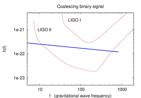
Figure 1: Noise curves $h_{\rm rms}(f)=\sqrt{fS_{h}(f)}$ for initial and next-generation LIGO interferometers noisecurveref (shown in thin lines) together with the signal strength $h_{c}(f)$ for an inspiralling binary of two $1.4M_{\odot}$ neutron stars at a distance of $200\,{\rm Mpc}$ (thick line) hcdef . The signal will terminate near the frequency of the innermost stable circular orbit, which is $\sim 850$ Hz as shown here if the neutron stars have radii of $10$ km and are modeled as $\Gamma=2$ polytropes Marronetti:2003hx . Resonantly excited modes can give rise to small but potentially measurable corrections to the phase of the waveform in the early portion $10\,{\rm Hz}\lesssim f\lesssim 100\,{\rm Hz}$ of the signal.

A third type of information potentially carried by the gravitational waves is the effect of the internal structure of the bodies on the early, low frequency ($10\,\text{Hz}\lesssim f\lesssim 100\,\text{Hz}$) portion of the signal, via the excitation of internal modes of oscillation of one of the neutron stars by the tidal gravitational field of its companion. In this regime the waveform’s phase evolution is dominated by the point-mass dynamics, and the perturbations due to the internal modes are small corrections. Nevertheless, if the accumulated phase shift due to the perturbations becomes of order unity or larger, it could impede the matched-filtering-based detection of NS-NS signals 1993PhRvL..70.2984C . Alternatively the detection of a phase perturbation could give information about the neutron star structure. For these reasons the excitation of neutron star modes has been studied in detail.

A given mode can be treated as a damped, driven harmonic oscillator, described by the equation

$${\ddot{q}}+\gamma{\dot{q}}+\omega_{\rm m}^{2}q=A(t)\cos[m\phi(t)].$$ (1)

Here $q$ is a generalized coordinate describing the mode, $\omega_{\rm m}$ is the mode frequency, $\gamma$ is a damping constant, $\phi(t)$ is the orbital phase of the binary, $m$ is the azimuthal quantum number of the mode, and $A(t)$ a slowly varying amplitude. As the inspiral of the binary proceeds, the orbital frequency $\omega={\dot{\phi}}$ gradually increases with time. Sufficiently early in the inspiral, therefore, the mode will be driven below resonance: $m\omega\ll\omega_{\rm m}$. Because the inspiral is adiabatic we also then have ${\dot{A}}/A\ll\omega_{\rm m}$ and ${\dot{\omega}}/\omega\ll\omega_{\rm m}$. Using these approximations Eq. (1) can be solved analytically in this pre-resonance regime, and one finds that the total energy absorbed by the mode up to time $t$ is

$$E(t)=\frac{A(t)^{2}}{2\omega_{\rm m}^{2}}+\gamma\int_{-\infty}^{t}dt^{\prime}\frac{\omega(t^{\prime})^{2}A(t^{\prime})^{2}}{\omega_{\rm m}^{4}/m^{2}+\omega(t^{\prime})^{2}\gamma^{2}}.$$ (2)

This energy absorption causes the orbit to inspiral slightly faster and changes the phase of the gravitational wave signal.

Mode excitations can have three different types of effects on the gravitational wave signal:

• Dissipative: There is a phase perturbation due to the second term in Eq. (2), corresponding to energy dissipated by the mode. This is a cumulative effect. It is dominated by the $l=2,m=\pm 2$ fundamental modes of the neutron star, and its magnitude depends on the size of the damping constant $\gamma$, which is determined by the fluid viscosity. This effect was examined by Bildsten and Cutler 1992ApJ…400..175B , who showed that the phase perturbation is negligible for all physically reasonable values of the viscosity.

• Adiabatic: There is a phase perturbation due to the first term in Eq. (2). This corresponds to the instantaneous energy present in the mode, as it adjusts adiabatically to sit at the minimum of its slowly-evolving potential. The perturbation to the waveform is again dominated by the $l=2,m=\pm 2$ fundamental modes 1995MNRAS.275..301K . This effect has been studied analytically in Refs. 1992ApJ…400..175B ; 1992ApJ…398..234K ; 1993ApJ…406L..63L ; 1998PhRvD..58h4012T ; Mora:2003wt and numerically in Refs. 1995MNRAS.275..301K ; 1994PThPh..91..871S ; 2001PhRvD..64j4007G ; 2002PhRvD..65j4021P ; 2002PhRvD..66f4013B . It can also be inferred from sequences of 3D numerical quasi-equilibrium models of NS-NS binaries 2002PhRvL..89w1102F ; Marronetti:2003gk ; Bejger:2004zx . The phase perturbation grows like $\omega(t)^{5/3}$ and is of order a few cycles by the end of inspiral. It may be marginally detectable for some nearby events Hinderer:2005 .

• Resonant: The frequencies of internal modes of a neutron star are typically of order $\omega_{\rm m}\sim\sqrt{M/R^{3}}$, where $M$ and $R$ are the stellar mass and radius. (We use units with $G=c=1$ throughout this paper). For a NS-NS binary, this is of order the orbital frequency at the end of the inspiral, $\sim 1000\,{\rm Hz}$. Therefore, most modes are driven at frequencies below their natural frequencies throughout the inspiral, and are never resonant. However, some mode do have frequencies $\omega_{\rm m}$ with $\omega_{\rm m}\ll\sqrt{M/R^{3}}$, and these modes are resonantly excited as the gradually increasing driving frequency $m\omega$ sweeps past $\omega_{\rm m}$. During resonance the effect of damping is negligible, and the width $\Delta\omega$ of the resonance is determined by the inspiral timescale. The energy deposited in the mode is thus enhanced compared to the equilibrium energy [the first term in Eq. (2)] by the ratio of the inspiral timescale to the orbital period. This can be a significant enhancement.

Resonant driving of modes in NS-NS binaries has been studied in Refs. 1994ApJ…426..688R ; 1994MNRAS.270..611L ; 1999MNRAS.308..153H ; 1995MNRAS.275..301K ; 2001PhRvD..64j4007G ; 2002PhRvD..65j4021P ; 2002PhRvD..66f4013B , and in the context of other binary systems in Refs. Willems:2002na ; 2003MNRAS.339…25R ; Rathore:2004gs ; Rathorethesis . One class of modes with suitably small frequencies are $g$-modes; however the overlap integrals for these modes are so small that the gravitational phase perturbation is small compared to unity 1995MNRAS.275..301K ; 1994ApJ…426..688R ; 1994MNRAS.270..611L . Another class are the $f$ and $p$-modes of rapidly rotating stars, where the inertial-frame frequency $\omega_{\rm m}$ can be much smaller than the corotating-frame frequency $\sim\sqrt{M/R^{3}}$. Ho and Lai 1999MNRAS.308..153H showed that the phase shifts due to these modes could be large compared to unity. However, the required NS spin frequencies are several hundred Hz, which is thought to be unlikely in inspiralling NS-NS binaries.

A third class of modes are Rossby modes ($r$-modes) 1981A&A….94..126P ; 1982ApJ…256..717S , for which the restoring force is dominated by the Coriolis force. For these modes the mode frequency $\omega_{\rm m}$ is of order the spin frequency of the star, and thus can be suitably small [$10\,\text{Hz}\lesssim\omega_{\text{ m}}/(2\pi)\lesssim 100\,\text{Hz}$]. Ho and Lai 1999MNRAS.308..153H computed the Newtonian driving of these modes, and showed that the phase shift is small compared to unity.

In this paper we compute the phase shift due to the post-Newtonian, gravitomagnetic resonant driving of the $r$-modes. Normally, post-Newtonian effects are much smaller than Newtonian ones. However, in this case the post-Newtonian effect is larger. The reason is that the Newtonian driving acts via a coupling to the mass quadrupole moment

$$Q_{ij}=\int d^{3}x\rho(x_{i}x_{j}-\frac{1}{3}\delta_{ij}{\bf x}^{2})$$ (3)

of the mode, where $\rho$ is the mass density. For $r$ modes, this mass quadrupole moment vanishes to zeroth order in the angular velocity $\Omega$ of the star; it is suppressed by a factor $\sim\Omega^{2}R^{3}/M$. By contrast, the gravitomagnetic driving acts via a coupling to the current quadrupole moment

$$S_{ij}=\frac{1}{2}\int d^{3}x\rho\left[({\bf x}\times{\bf v})_{i}x_{j}+({\bf x}\times{\bf v})_{j}x_{i}\right],$$ (4)

where ${\bf v}$ is the velocity of the fluid. This current quadrupole moment is nonvanishing to zeroth order in $\Omega$, and the gravitomagnetic coupling is therefore enhanced over the Newtonian tidal coupling by a factor of $\sim\Omega^{2}R^{3}/M$. This enhancement factor can exceed the usual factor $\sim v^{2}/c^{2}$ by which post-Newtonian effects are suppressed, where $v$ is a velocity scale. It is for this same reason that the radiation-reaction induced instability of $r$-modes in newly born neutron stars 1998ApJ…502..708A ; 1998ApJ…502..714F is dominated by the gravitomagnetic coupling and not the mass quadrupole coupling.

I.2 Effect of resonance on gravitational wave signal

We now discuss the observational signature of a mode resonance in the gravitational wave signal. We denote by $\Phi(t)$ the phase of the waveform, which is twice the orbital phase $\phi(t)$. We denote by $\Phi_{\rm pp}(t)$ the phase that one obtains from a point particle model, neglecting the effects of the internal modes of the stars. To the leading post-Newtonian order, this point-particle phase is given from the quadrupole formula by the differential equation Peters:1963ux

$${\dot{\omega}}=\frac{96}{5}\mu M_{\rm t}^{2/3}\omega^{11/3},$$ (5)

where $\omega={\dot{\phi}}$ is the orbital angular velocity, and $M_{\rm t}$ and $\mu$ are the total mass and reduced mass of the binary.

Consider now the phase $\Phi(t)$ including the effect of the mode. We neglect the phase shift caused by the adiabatic response of the mode at early times before the resonance [the first term in Eq. (2)], as this phase shift is small compared to the effect of the resonance. We also neglect the cumulative phase shift due to damping. Therefore at early times we have $\Phi(t)=\Phi_{\rm pp}(t)$. The duration of the resonance is short compared to the inspiral timescale (see Sec. I.3 below). After the resonance, the mode again has a negligible influence on the orbit of the binary, and Eq. (5) applies once more. However, the two constants of integration that arise when solving Eq. (5) need not match between the pre-resonance and post-resonance waveforms. Therefore, the phase can be written as

$$\Phi(t)=\left\{\begin{array}[]{ll}\Phi_{\rm pp}(t)&\mbox{ $t-t_{0}\ll-t_{\rm res}$,}\\ \Phi_{\rm pp}(t+\Delta t)-\Delta\Phi&\mbox{ $t-t_{0}\gg t_{\rm res}$.}\\ \end{array}\right.$$ (6)

Here $t_{0}$ is the time at which resonance occurs, and $t_{\rm res}$ is the duration of the resonance. The effect of the resonance is thus to cause an overall phase shift $\Delta\Phi$, and also to cause a time shift $\Delta t$ in the signal. If energy is absorbed by the mode, then the inspiral proceeds more quickly and $\Delta t$ is positive.

It turns out that the two parameters $\Delta t$ and $\Delta\Phi$ characterizing the effect of the resonance are not independent. To a good approximation they are related by

$$\Delta\Phi={\dot{\Phi}}_{\rm pp}(t_{0})\Delta t,$$ (7)

as argued by Reisenegger and Goldreich 1994ApJ…426..688R , and as derived in detail in Sec. IV below. Inserting this relation into Eq. (6) and expanding to linear order in the small parameter $\Delta t$ yields for the late-time phase

$$\Phi(t)=\Phi_{\rm pp}(t)+\left[{\dot{\Phi}}_{\rm pp}(t)-{\dot{\Phi}}_{\rm pp}(t_{0})\right]\Delta t.$$ (8)

The physical meaning of the condition (7) is thus that the resonance can be idealized as an instantaneous change in frequency at $t=t_{0}$ with no corresponding instantaneous change in phase. Rewriting the phase (8) in terms of $\Delta\Phi$ using (7) and using ${\dot{\Phi}}_{\rm pp}=2\omega$ gives

$$\Phi(t)=\Phi_{\rm pp}(t)+\left[\frac{\omega(t)}{\omega_{0}}-1\right]\Delta\Phi,$$ (9)

where $\omega_{0}=\omega(t_{0})$ is the orbital frequency at resonance. The phase perturbation due to the resonance therefore grows with time after the resonance, and can become much larger than $\Delta\Phi$ when $\omega\gg\omega_{0}$.

One can alternatively think of the phase correction as being non-zero before the resonance, and zero afterwards 1994ApJ…426..688R . This is what would be perceived if one matched a template with the portion of the observed waveform after the resonance. In other words, if we define a point-particle waveform phase ${\tilde{\Phi}}_{\rm pp}(t)$ with different conventions for the starting time and starting phase via

$${\tilde{\Phi}}_{\rm pp}(t)\equiv\Phi_{\rm pp}(t+\Delta t)-\Delta\Phi,$$ (10)

then we obtain

$$\Phi(t)=\left\{\begin{array}[]{ll}{\tilde{\Phi}}_{\rm pp}(t)-\left[\frac{\omega(t)}{\omega_{0}}-1\right]\Delta\Phi&\mbox{\ \ $t-t_{0}\ll-t_{\rm res}$,}\\ {\tilde{\Phi}}_{\rm pp}(t)&\mbox{\ \ $t-t_{0}\gg t_{\rm res}$.}\\ \end{array}\right.$$ (11)

The phase correction $\Phi-{\tilde{\Phi}}_{\rm pp}$ is now a linear function of frequency, interpolating between $\Delta\Phi$ at $\omega=0$ to zero at resonance $\omega=\omega_{0}$. Since this phase correction never exceeds $\Delta\Phi$, we see that the detectability criterion for the resonance effect is $\Delta\Phi\gtrsim 1$. Thus, the phase shifts $\gg\Delta\Phi$ predicted by Eq. (9) are fictitious in the sense that they are not measurable.

I.3 Order of magnitude estimates

We now turn to an order of magnitude estimate of the mode excitation and the phase shift $\Delta\Phi$, both for the Newtonian driving studied previously and for the gravitomagnetic driving.

We consider a star of mass $M$ and radius $R$ with a companion of mass $M^{\prime}$. The orbital angular velocity at resonance is $\omega_{0}$; this is also the mode frequency (up to a factor of the azimuthal quantum number $m$ which we neglect here). The separation $r$ of the two stars at resonance is then given by $\omega_{0}^{2}\sim M_{\rm t}/r^{3}$, where $M_{\rm t}=M+M^{\prime}$ is the total mass.

Let the magnitude of the tidal acceleration be $a_{\rm tid}$, and let the duration of the resonance be $t_{\rm res}$. The mode can be treated as a harmonic oscillator of mass $\sim M$ and frequency $\omega_{0}$. During the resonance, the mode absorbs energy at the same rate as a free particle would, so the total energy absorbed is

$$\Delta E\sim Ma_{\rm tid}^{2}t_{\rm res}^{2}.$$ (12)

Now the gravitational wave luminosity ${\dot{E}}_{\rm gw}$ is to a good approximation unaffected by the resonance. Therefore the loss of energy $\Delta E$ from the orbit decreases the time taken to inspiral by an amount $\Delta t=\Delta E/{\dot{E}}_{\rm gw}$. From Eq. (7) the corresponding phase shift is $\Delta\Phi\sim\Delta t/t_{\rm orb}$, where $t_{\rm orb}\sim 1/\omega_{0}$ is the orbital period. This gives

$$\Delta\Phi\sim\frac{t_{\rm rr}\Delta E}{t_{\rm orb}E_{\rm orb}},$$ (13)

where $E_{\rm orb}$ is the orbital energy and $t_{\rm rr}$ is the radiation reaction timescale. This phase shift is just the energy absorbed divided by the energy radiated per orbit.

Next, using $E_{\rm orb}\sim MM^{\prime}/r$ and the formula (12) for $\Delta E$ gives

$$\Delta\Phi\sim\frac{r}{M^{\prime}}a_{\rm tid}^{2}\frac{t_{\rm res}^{2}t_{\rm rr}}{t_{\rm orb}}.$$ (14)

The resonance time $t_{\rm res}$ is the geometric mean of the orbital and radiation reaction times $t_{\rm orb}$ and $t_{\rm rr}$. This follows from the fact that the orbital phase near resonance can be expanded as

$$\phi\sim\phi_{0}+\omega_{0}(t-t_{0})+\frac{\omega_{0}}{t_{\rm rr}}(t-t_{0})^{2}+\ldots,$$ (15)

from the definition of the radiation reaction timescale $t_{\rm rr}$. The mode is resonant when the quadratic term in Eq. (15) is small compared to unity, so that the force on the mode is in phase with the mode’s natural oscillation. This gives $t_{\rm res}\sim\sqrt{t_{\rm orb}t_{\rm rr}}$, and we get

$$\Delta\Phi\sim\frac{r}{M^{\prime}}a_{\rm tid}^{2}t_{\rm rr}^{2}.$$ (16)

Finally, we use the scaling $t_{\rm rr}\sim r^{4}/(\mu M_{\rm t}^{2})$ for the radiation reaction time given by the quadrupole formula, where $\mu$ is the reduced mass. This gives

$$\Delta\Phi\sim\frac{r^{9}}{M^{\prime}\mu^{2}M_{\rm t}^{4}}a_{\rm tid}^{2}.$$ (17)

We now consider various different cases. For the Newtonian driving of a mode via a tidal field of multipole of order $l$, we have

$$a_{\rm tid}\sim\frac{M^{\prime}}{r^{2}}\left({\frac{R}{r}}\right)^{l-1}.$$ (18)

[The leading order, quadrupolar driving is $l=2$.] Inserting this into Eq. (17) and eliminating $r$ using $\omega_{0}^{2}r^{3}\sim M_{\rm t}$ gives

$$\Delta\Phi\sim\left(\frac{M^{3}}{\mu M_{\rm t}^{2}}\right)\left(\frac{R}{M}\right)^{5}\left(\frac{\omega_{0}^{2}}{M/R^{3}}\right)^{(l-5)/3},$$ (19)

which agrees with previous analyses 1994ApJ…426..688R ; 1994MNRAS.270..611L for $g$ and $f$ modes.

For the Newtonian driving of $r$-modes, the leading order driving is $l=3$ rather than $l=2$ 1999MNRAS.308..153H . Also the tidal acceleration $a_{\rm tid}$ should be multiplied by the suppression factor $\omega_{0}^{2}R^{3}/M$ discussed in Sec. I.1 above, and the final phase shift (19) should be multiplied by the square of this factor. This gives in the equal mass case $M=M^{\prime}$

$$\Delta\Phi\sim\frac{R^{10}\omega_{0}^{10/3}}{M^{20/3}}.$$ (20)

Now the frequency $m\omega_{0}$ of the dominant, $l=m=2$ $r$-mode is related to the spin frequency $f_{\rm spin}$ of the neutron star by $2\omega_{0}=8\pi f_{\rm spin}/3$, so we obtain

$$\Delta\Phi=k\frac{R^{10}f_{\rm spin}^{10/3}}{M^{20/3}},$$ (21)

where $k$ is a dimensionless constant of order unity. Equation (21) agrees with the results of Ho and Lai 1999MNRAS.308..153H , who show that $k\approx 0.4$ for a $\Gamma=2$ polytrope, and for the $l=m=2$ $r$-mode. This gives

$$\Delta\Phi_{\rm r-mode,N}=8\times 10^{-5}R_{10}^{10}f_{s100}^{10/3}M_{1.4}^{-20/3},$$ (22)

where the subscript N denotes Newtonian and we have defined $R=10R_{10}\,{\rm km}$, $M=1.4M_{1.4}M_{\odot}$, and $f_{\rm spin}=100f_{s100}\,{\rm Hz}$.

For the gravitomagnetic driving of $r$-modes, the tidal acceleration is given by

$$a_{\rm tid}\sim\left(\frac{M^{\prime}R}{r^{3}}\right)v_{\rm spin}v_{\rm orb}.$$ (23)

Here the first factor in brackets is tidal acceleration (18) for Newtonian quadrupolar $l=2$ driving. Since the interaction is gravitomagnetic, it is suppressed by two powers of velocity relative to the Newtonian interaction. One power of velocity is associated with the source of the gravitomagnetic field, and is the orbital velocity $v_{\rm orb}\sim\omega_{0}r$. The second power of velocity is that coming from the Lorentz-type ${\bf v}\times{\bf B}$ force law, and is the internal fluid velocity in the neutron star due to its spin, $v_{\rm spin}\sim\omega_{0}R$. Combining these estimates with Eq. (17) and eliminating $\omega_{0}$ in favor of $f_{\rm spin}$ gives

$$\Delta\Phi\sim\frac{R^{4}f_{\rm spin}^{2/3}}{M^{\prime}M^{2}M_{\rm t}^{1/3}}.$$ (24)

In the equal mass case $M=M^{\prime}$ this gives

$$\Delta\Phi_{\rm r-mode,PN}\sim 3.4\ R_{10}^{4}f_{s100}^{2/3}M_{1.4}^{-10/3}.$$ (25)

Here the subscript PN denotes post-Newtonian.

I.4 Results and implications

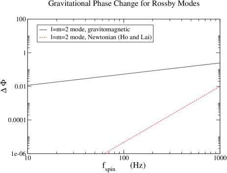
Figure 2: The magnitude of the gravitational-wave phase shift $\Delta\Phi$ due to the $r$-mode resonance as a function of the spin frequency $f_{\rm spin}$ of the neutron star, for both the Newtonian and gravitomagnetic driving, for a binary with masses $M=M^{\prime}=1.4M_{\odot}$, and for a neutron star radius of $R=10\,{\rm km}$. The star is modeled as a $\Gamma=2$ polytrope. The mode plotted is $l=2$, $m=2$ in each case. The angle $\psi$ between the spin and the orbital angular momentum has been chosen in each case to maximize the phase shift; $\psi$ is $34.4^{\circ}$ in the Newtonian case and $60^{\circ}$ in the post-Newtonian case. The resonance occurs at an orbital frequency of $4f_{\rm spin}/9$ in the Newtonian case and at $4f_{\rm spin}/3$ in the post-Newtonian case. The corresponding gravitational wave frequencies are $8f_{\rm spin}/9$ and $8f_{\rm spin}/3$ respectively. It can be seen that the gravitomagnetic driving dominates.

The fact that the order-of-magnitude estimate (25) of the phase shift is of order unity, and thus potentially detectable in the gravitational wave signal via matched filtering 1993PhRvL..70.2984C , is the primary motivation for the computation of this paper. We compute the dimensionless coefficient in Eq. (24), and find for the case of a $\Gamma=2$ polytrope for the $l=2$, $m=2$ mode [cf. Eq. (138) below, multiplied by two to convert from orbital phase shift $\Delta\phi$ to gravitational wave phase shift $\Delta\Phi$]

$$\Delta\Phi_{\rm r-mode,PN}=-0.06\ R_{10}^{4}f_{s100}^{2/3}M_{1.4}^{-10/3}.$$ (26)

This is somewhat smaller than the estimate (25). Figure 2 compares this result to the Newtonian phase shift (22). In Table 1 we show the phase shift $\Delta\Phi_{22}=2\Delta\phi_{22}$ that will occur at coalescence for the five known double neutron star binaries. For B1913+16 we used the known value $\psi=22^{\circ}$ of the angle between the pulsar spin and the orbital angular momentum 1998ApJ…509..856K , and for the remaining binaries for which $\psi$ is unknown we took an average of the angular factors appearing in the phase lag (133b). We assumed a $\Gamma=2$ polytrope equation of state and a radius of 10 km for all pulsars.

System	spin period	$M$	$M^{\prime}$	phase lag $\Delta\Phi_{22}$
B1913+16	59.0	1.441	1.387	-0.005
B1534+12	37.9	1.339	1.339	-0.009
B2127+11C	30.5	1.358	1.354	-0.010
J0737-3039	22.7	1.34	1.25	-0.013
J1756-2251	28.5	1.40	1.18	-0.011

Table 1: List of gravitational wave phase lag parameters that will occur for the $l=2,m=2$ resonance for the known double neutron star binaries when they coalesce. For B1913+16, the known value for the misalignment angle $\psi$ ($22^{\circ}$) was used; for the others, the average value of the angular factors was used. The pulsar mass $M$ and companion mass $M^{\prime}$ are in solar masses and the pulsar spin period is in milliseconds. The parameter values were taken from Ref. 2005LRR…..8….7L .

The phase shift (26) is sufficiently small that it is unlikely to be detectable in the gravitational wave signal for most detected binary inspirals. Even for the most favorable conceivable neutron star parameters of $M=1.0\,M_{\odot}$ and $R=15\,{\rm km}$, the phase shift is $\sim 0.8$ radians. An analysis of the detectability of mode resonances indicates that the minimum detectable value of $\Delta\Phi$ is $\Delta\Phi\sim 2$ for $f_{\rm spin}=100\,{\rm Hz}$ at a signal to noise ratio of $S/N=10$ Balachandran:2005 . Therefore the minimum signal to noise ratio necessary for detection of the effect is between $\sim 30$ and $\sim 300$, depending on the neutron star parameters. It is conceivable that the effect could be detected in some of the closest detected binary inspirals with advanced interferometers.

One of the interesting features of the interaction is that the phase shift is negative, corresponding to energy being transferred from the star to the orbit rather than the other way around. This arises because the star is rotating and the interaction reduces the spin of the star, tapping into its rotational kinetic energy. In Sec. IV.2 below we show that this sign of energy transfer is only possible for modes which satisfy the Chandrasekhar-Friedman-Schutz mode instability criterion 1970PhRvL..24..762C ; 1978ApJ…222..281F of being retrograde in the corotating frame and prograde in the inertial frame.

Although the $r$-mode resonance may not be detectable, it is nevertheless probably the strongest of all the mode resonances in the early phase of the gravitational wave signal. The energy transfer corresponding to the phase shift (26) is from Eq. (13)

$$\Delta E\sim(1.4\times 10^{48}\,{\rm erg})\,R_{10}^{4}f_{s100}^{3},$$ (27)

which is fairly large. The corresponding dimensionless amplitude $\alpha$ of the $r$-mode in the notation of Ref. prl…80…4843 is

$$\alpha\sim 0.3\,R_{10}^{2}f_{s100}M_{1.4}^{-1}.$$ (28)

This amplitude is sufficiently large that nonlinear mode-mode interactions should be important, as in the case of unstable $r$-modes in newly born neutron stars and in low mass X-ray binaries prl…80…4843 . In those contexts the mode-mode coupling causes the mode growth to saturate at $\alpha\sim 10^{-4}$ Schenk:2001zm ; Morsink:2002ut ; Arras:2002dw ; Brink:2004bg ; Brink:2004qf ; Brink:2004kt . Here however the $r$-mode is driven on much shorter timescales, and the mode-mode coupling likely does not have time to operate efficiently. It is possible that the type of nonlinear effects studied numerically in Refs. Gressman:2002zy ; Lindblom:2001sg (generation of differential rotation, shocks, wave breaking) could occur.

I.5 Organization of this paper

The remainder of this paper is organized as follows. In Secs. II, III and IV we analyze resonant driving of modes in Newtonian gravity, building on the previous studies of Refs. 1994ApJ…426..688R ; 1994MNRAS.270..611L ; 1999MNRAS.308..153H ; Rathore:2004gs ; Rathorethesis . The time delay parameter $\Delta t$ can be derived using energy conservation which we discuss in Appendix B, but the relation (7) between the phase shift parameter $\Delta\Phi$ and $\Delta t$ requires an analysis of the orbital equations of motion, which we give in Sec. IV. In Sec. V and Appendix A we show that the gravitomagnetic driving of modes can be computed to leading order using Newtonian stellar perturbation theory supplemented by a gravitomagnetic external acceleration, and we deduce the phase shifts generated by the driving of $r$-modes.

II Newtonian mode-orbit coupling

In this section we describe a model dynamical system that describes the Newtonian excitation of modes in inspiralling binary systems. We generalize previous treatments Rathore:2004gs ; Rathorethesis to allow for stellar rotation. The dynamical system will actually be general enough to encompass the post-Newtonian driving of $r$-modes, as we discuss in Sec. V below.

II.1 Mode expansions in rotating Newtonian stars

We start by reviewing the evolution equations for mode amplitudes in rotating Newtonian stars, following the treatment in Ref. Schenk:2001zm . We assume that the background star is uniformly rotating with angular velocity ${\bf\Omega}$ and mass $M$. We denote by $(\bm{x},t)$ the inertial frame coordinates and by $(\bar{{\bm{x}}},t)$ the co-rotating frame coordinates. These coordinate systems are oriented so that ${\bf\Omega}$ is in the $z$ direction. Below we will use spherical polar coordinates $(r,\theta_{s},\bar{\phi_{s}})$ for $\bar{{\bm{x}}}$; the corresponding inertial frame coordinates are $(r,\theta_{s},\phi_{s})$ where

$${\phi_{s}}=\bar{\phi}_{s}+\Omega t.$$ (29)

A mode of a rotating star is a pair $(\bm{\xi}(\bar{{\bm{x}}}),\omega)$ of a mode function $\bm{\xi}(\bar{{\bm{x}}})$ and a rotating-frame frequency $\omega$, such that the rotating-frame Lagrangian displacement given by

$$\bm{\xi}(\bar{{\bm{x}}},t)=\bm{\xi}(\bar{{\bm{x}}})e^{-i\omega t}$$ (30)

is a solution to the linearized hydrodynamic equations. We label the different modes with $\omega\leq 0$ by an index $j$; the $j$th mode is $(\bm{\xi}_{j}(\bar{{\bm{x}}}),\omega_{j})$. It can then be shown that the Lagrangian displacement $\bm{\xi}(\bar{{\bm{x}}},t)$ and its time derivative ${\dot{\bm{\xi}}}(\bar{{\bm{x}}},t)$ can be expanded in the phase-space mode expansion Schenk:2001zm

$$\left[\begin{array}[]{c}\bm{\xi}\\ \dot{\bm{\xi}}\end{array}\right]=\sum_{j}c_{j}(t)\left[\begin{array}[]{c}\bm{\xi}_{j}\\ -i\omega_{j}\bm{\xi}_{j}\end{array}\right]+c^{\ast}_{j}(t)\left[\begin{array}[]{c}\bm{\xi}^{\ast}_{j}\\ i\omega_{j}\bm{\xi}^{\ast}_{j}\end{array}\right].$$ (31)

In rotating stars, one cannot in general find a basis of modes which are real, so the expansion coefficients $c_{j}(t)$ are complex in general.

If there is an external acceleration $\bm{a}_{\text{ext}}(\bar{{\bm{x}}},t)$ acting on the star, then the equation of motion for the $j$th mode is Schenk:2001zm

$$\dot{c}_{j}+i\omega_{j}c_{j}=\frac{i}{b_{j}}\langle\bm{\xi}_{j},\bm{a}_{\text{ext}}\rangle,$$ (32)

where the inner product is defined by

$$\langle\bm{\xi}_{j},\bm{a}_{\text{ext}}\rangle=\int d^{3}\bar{x}\,\rho\,\bm{\xi}_{j}^{\ast}\cdot\bm{a}_{\text{ext}}$$ (33)

and $\rho(\bar{{\bm{x}}})$ is the background density. The constant $b_{j}$ is given by

$$b_{j}=\langle\bm{\xi}_{j},2\omega_{j}\bm{\xi}_{j}+2i{\bf\Omega}\times\bm{\xi}_{j}\rangle.$$ (34)

We normalize the modes using the convention

$$\langle\bm{\xi}_{j},\bm{\xi}_{j}\rangle=MR^{2},$$ (35)

where $R$ is the stellar radius.

An equivalent second-order form of the equation of motion can be obtained by differentiating Eq. (32) and eliminating ${\dot{c}}_{j}$ in the result using Eq. (32). This gives

$${\ddot{c}}_{j}+\omega_{j}^{2}c_{j}={\dot{f}}_{j}-i\omega_{j}f_{j},$$

where $f_{j}(t)\equiv i\langle\bm{\xi}_{j},\bm{a}_{\text{ext}}\rangle/b_{j}.$ This is the form of the equation of motion discussed in the Introduction, cf. Eq.  (1).

II.2 Mode-orbit coupling equations

We now consider a binary system of a star of mass $M$, whose modes are excited, and a companion of mass $M^{\prime}$ which we treat as a point mass. We denote the total mass $M+M^{\prime}$ by $M_{\rm t}$, and the reduced mass $MM^{\prime}/M_{\rm t}$ by $\mu$. We denote by ${\bm{x}}=(r,\theta,\phi)$ the displacement of $M^{\prime}$ with respect to $M$ in polar coordinates. We orient these polar coordinates so that the motion is confined to the equatorial plane $\theta=\pi/2$. The equations of motion describing this system are

$$\dot{c}_{j}+i\omega_{j}c_{j}=f_{j},$$ (36a)

$${\ddot{r}}-r{\dot{\phi}}^{2}+\frac{M_{\rm t}}{r^{2}}=a_{\hat{r}}^{\text{modes}}+a_{\hat{r}}^{\text{diss}},$$ (36b)

$$r{\ddot{\phi}}+2{\dot{r}}{\dot{\phi}}=a_{\hat{\phi}}^{\text{modes}}+a_{\hat{\phi}}^{\text{diss}}.$$ (36c)

Here $c_{j}$ and $\omega_{j}$ are the amplitude and rotating-frame frequency of the $j$th mode. The right hand sides of Eqs. (36b) and (36c) are the components of the total relative acceleration ${\bm{a}}^{\text{modes}}+{\bm{a}}^{\text{diss}}$ on the orthornomal basis ${\bm{e}}_{\hat{r}}$, ${\bm{e}}_{\hat{\phi}}$, where $\bm{a}^{\text{modes}}$ describes the back-reaction of excited modes onto orbital motion and $\bm{a}^{\text{diss}}$ is the back-reaction of emission of gravitational radiation onto orbital motion. The latter acceleration term is obtained from the Burke-Thorne radiation-reaction acceleration mtw

$$a_{i}^{\rm diss}(t,{\bf x})=-\frac{2}{5}\frac{d^{5}Q^{\rm TF}_{ij}}{dt^{5}}(t)x_{j},$$ (37)

where $Q_{ij}$ is the quadrupole moment of the binary and TF means trace-free part. In evaluating this expression we include only the contribution $Q_{ij}=\mu x_{i}x_{j}$ to the quadrupole from the orbital degrees of freedom, neglecting the contribution from the modes. To evaluate the time derivatives of $Q_{ij}$ we use the Newtonian orbital equations of motion with the mode coupling terms omitted. We also neglect the effect of gravitational wave damping on the modes themselves. This yields the components of the dissipative acceleration

$$a^{\rm diss}_{\hat{r}}=\frac{16\mu M_{\rm t}}{5r^{3}}{\dot{r}}\left[{\dot{r}}^{2}+6r^{2}{\dot{\phi}}^{2}+\frac{4M_{\rm t}}{3r}\right]$$ (38)

and

$$a^{\rm diss}_{\hat{\phi}}=\frac{8\mu M_{\rm t}}{5r^{2}}{\dot{\phi}}\left[9{\dot{r}}^{2}-6r^{2}{\dot{\phi}}^{2}+\frac{2M_{\rm t}}{r}\right].$$ (39)

The function $f_{j}$ in Eq. (36a) describes the coupling between mode $j$ and the tidal gravitational field of the companion object. For Newtonian mode-orbit coupling, it can be derived as follows 1999MNRAS.308..153H . Insert into the right hand side of Eq. (32) the acceleration ${\bm{a}}_{\rm ext}=-{\bm{\nabla}}\Phi_{\rm ext}$, where the external potential is

$$\Phi_{\rm ext} = -\bm{\nabla}\frac{M^{\prime}}{|{\bm{x}}-{\bm{x}}(t)|}$$

$$= -M^{\prime}\sum_{l^{\prime}=2}^{\infty}\sum_{m^{\prime}=-l^{\prime}}^{l^{\prime}}W_{l^{\prime}m^{\prime}}\frac{r^{l}e^{-im^{\prime}\phi(t)}}{r(t)^{l+1}}Y_{l^{\prime}m^{\prime}}(\theta,\phi).$$

Here the coefficient $W_{l^{\prime}m^{\prime}}$ is given by Eq. (2.2) of Ref. 1999MNRAS.308..153H , and ${\bm{x}}(t)=(r(t),\pi/2,\phi(t))$ is the location of the companion. The spherical harmonics that appear in Eq. (LABEL:phiext) are related to to spherical harmonics of the inertial-frame coordinates $(r,\theta_{s},\phi_{s})$ which are aligned with the spin axis of the star by

$$Y_{l^{\prime}m^{\prime}}(\theta,\phi)=\sum_{m}{\cal D}^{(l^{\prime})}_{mm^{\prime}}Y_{l^{\prime}m}(\theta_{s},\phi_{s}),$$ (41)

where ${\cal D}^{(l^{\prime})}_{mm^{\prime}}$ is the Wigner ${\cal D}$-function 1999MNRAS.308..153H . Finally use the relation (29) between the inertial and corotating frame coordinates $\phi_{s}$ and ${\bar{\phi}}_{s}$. The result is

$$f_{j}=\sum_{l^{\prime}m^{\prime}}Q_{j,l^{\prime}m^{\prime}}\,\frac{e^{-im^{\prime}\phi(t)+im_{j}\Omega t}}{r(t)^{l^{\prime}+1}},$$ (42)

where $m_{j}$ is the azumithal quantum number of the mode $\bm{\xi}_{j}$, and

$$Q_{j,l^{\prime}m^{\prime}}=\frac{iM^{\prime}}{b_{j}}W_{l^{\prime}m^{\prime}}{\cal D}^{(l^{\prime})}_{m_{j}m^{\prime}}\left<\bm{\xi}_{j},\bm{\nabla}[r^{l^{\prime}}Y_{l^{\prime}m_{j}}(\theta_{s},{\bar{\phi}}_{s})]\right>.$$ (43)

Note that there are two different azimuthal quantum numbers in the final expression (42), the quantum number $m_{j}$ of the mode which controls the number of factors of the phase $e^{i\Omega t}$, and the quantum number $m^{\prime}$ which controls the number of factors of the phase $e^{-i\phi(t)}$. These two quantum numbers coincide when the spin axis of the star is aligned with the orbital angular momentum, but not in general.

For the Newtonian case, in the absence of dissipation, the dynamical system (36) can be derived from the Hamiltonian

$$H=\frac{p_{r}^{2}}{2\mu}+\frac{p_{\phi}^{2}}{2\mu r^{2}}-\frac{\mu M_{t}}{r}+\sum_{j}b_{j}\left[\omega_{j}|c_{j}|^{2}+if_{j}c_{j}^{*}-if_{j}^{*}c_{j}\right],$$ (44)

where $p_{r}=\mu{\dot{r}}$, $p_{\phi}=\mu r^{2}{\dot{\phi}}$, together with the Poisson brackets $\{c_{j},c_{k}\}=0$, $\{c_{j},c_{k}^{*}\}=-i\delta_{jk}/b_{j}$. This allows us to read off the orbital acceleration $\bm{a}^{\text{modes}}$ due to the modes:

$$a_{\hat{r}}^{\text{modes}} = \frac{i}{\mu}\sum_{j}b_{j}\left(c_{j}\frac{\partial f_{j}^{*}}{\partial r}-c_{j}^{*}\frac{\partial f_{j}}{\partial r}\right),$$ (45a)

$$a_{\hat{\phi}}^{\text{modes}} = \frac{i}{\mu r}\sum_{j}b_{j}\left(c_{j}\frac{\partial f_{j}^{*}}{\partial\phi}-c_{j}^{*}\frac{\partial f_{j}}{\partial\phi}\right).$$ (45b)

From the formula (42) we see that a given mode $j$ is driven by a sum of terms labeled by $(l^{\prime},m^{\prime})$, the effects of which superpose linearly. For the remainder of this section and in Secs. III and IV we will focus attention on a particular mode $j$ and on a particular driving term $(l^{\prime},m^{\prime})$. Using the notations $A_{j}(r)=|Q_{j,l^{\prime}m^{\prime}}|/r^{l^{\prime}+1}$ and $e^{i\chi_{j}}=Q_{j,l^{\prime}m^{\prime}}/|Q_{j,l^{\prime}m^{\prime}}|$, the coupling function (42) and the orbital acceleration (45b) can be written as

$$f_{j} = A_{j}[r(t)]\,e^{-im^{\prime}\phi(t)+im_{j}\Omega t+i\chi_{j}},$$ (46a)

$$a_{\hat{\phi}}^{\text{modes}} = -\frac{2m^{\prime}b_{j}A_{j}[r(t)]}{\mu r(t)}\Re\left[c_{j}^{*}e^{-im^{\prime}\phi(t)+im_{j}\Omega t+i\chi_{j}}\right].$$

Although these formulae (46) were derived for Newtonian tidal driving, we shall see in Sec. V below that they also apply to gravitomagnetic driving in the vicinity of a resonance, with appropriate choices of the functions $A_{j}(r)$ and phases $\chi_{j}$.

II.3 New orbital variables

In order to analyze the effects of the mode coupling on the orbital motion it is useful to make a change of variables, from $r(t)$, $\phi(t)$, ${\dot{r}}(t)$, ${\dot{\phi}}(t)$ to new variables $p(t)$, $\phi(t)$, $e(t)$ and $\phi_{0}(t)$ that characterize the Newtonian ellipse that is instantaneously tangent to the orbit. Here $p$ is the instantaneous semilatus rectum and $e$ is the instantaneous eccentricity. These variables are defined by the equations

$$r = \frac{p}{1+ec_{\phi}},$$ (47a)

$${\dot{r}} = \sqrt{\frac{M_{\rm t}}{p}}es_{\phi},$$ (47b)

$${\dot{\phi}} = \sqrt{\frac{M_{\rm t}}{p^{3}}}\left[1+ec_{\phi}\right]^{2},$$ (47c)

where $c_{\phi}=\cos(\phi-\phi_{0})$ and $s_{\phi}=\sin(\phi-\phi_{0})$. In terms of these variables the orbital equations become

$${\dot{p}} = \frac{2p^{3/2}}{\sqrt{M_{\rm t}}(1+ec_{\phi})}a_{\hat{\phi}}$$ (48a)

$${\dot{\phi}} = \frac{\sqrt{M_{\rm t}}}{p^{3/2}}(1+ec_{\phi})^{2},$$ (48b)

$${\dot{e}} = \frac{\sqrt{p}}{2\sqrt{M_{\rm t}}(1+ec_{\phi})}$$ (48c)

$$\times\bigg{[}(3e+4c_{\phi}+ec_{2\phi})a_{\hat{\phi}}+(2s_{\phi}+es_{2\phi})a_{\hat{r}}\bigg{]},$$

$${\dot{\phi}}_{0} = \frac{-\sqrt{p}}{2e\sqrt{M_{\rm t}}(1+ec_{\phi})}$$

$$\times\bigg{[}(e+2c_{\phi}+ec_{2\phi})a_{\hat{r}}-(4s_{\phi}+es_{2\phi})a_{\hat{\phi}}\bigg{]}.$$

Here $c_{2\phi}=\cos[2(\phi-\phi_{0})]$, $s_{2\phi}=\sin[2(\phi-\phi_{0})]$, and $a_{\hat{r}}=a_{\hat{r}}^{\text{modes}}+a_{\hat{r}}^{\text{diss}}$ and $a_{\hat{\phi}}=a_{\hat{\phi}}^{\text{modes}}+a_{\hat{\phi}}^{\text{diss}}$ are the components of the total acceleration in the radial and tangential directions.

II.4 The circular approximation

In this paper we restrict attention to situations where the eccentricity $e$ is negligibly small before, during and after the mode resonance. We will justify this assumption in Sec. IV.3 below by estimating the magnitude of the eccentricity generated during the resonance. Using this approximation we can simplify the set of equations as follows. We can drop Eqs. (48c) and (LABEL:eq:phi0dot00), and we simplify the remaining equations (36a), (48a), and (48b) using $e=0$. Using the expressions (38) and (39) for the dissipative components of the acceleration, and the mode-orbit coupling terms (46), now gives

$$\dot{c}_{j}+i\omega_{j}c = A_{j}(p)\,e^{-im^{\prime}\phi(t)+im_{j}\Omega t+i\chi_{j}},$$ (49a)

$${\dot{p}}+\frac{64\mu M_{\rm t}^{2}}{5p^{3}} = -\frac{4m^{\prime}b_{j}A_{j}(p)\sqrt{p}}{\mu\sqrt{M_{\rm t}}}$$ (49b)

$$\times\Re\left[c_{j}^{*}e^{-im^{\prime}\phi(t)+im_{j}\Omega t+i\chi_{j}}\right],\ \ \ \$$

$${\dot{\phi}}-\frac{\sqrt{M_{\rm t}}}{p^{3/2}} = 0.$$ (49c)

Note that only the $\phi$ component of the acceleration contributes in this approximation.

II.5 The no-backreaction approximation

When the amplitude of the mode coupling $A_{j}$ is small we can solve the system (49) of equations by neglecting the backreaction of the mode excitation on the orbital motion. More precisely, we (i) solve the orbital equations (49b) and (49c) for the zeroth order solutions $p(t)$ and $\phi(t)$, neglecting the mode coupling; (ii) insert those zeroth order solutions into Eq. (49a) to compute the evolution of the mode amplitude $c(t)$; and (iii) insert that mode amplitude $c(t)$ into Eqs. (49b) and (49c) to obtain the linearized perturbations $\delta p(t)$ and $\delta\phi(t)$ to the orbital motion. Steps (i) and (ii) are carried out in Sec. III, where we extend previous results in the vicinity of resonance by Rathore, Blandford and Broderick Rathore:2004gs ; Rathorethesis . Step (iii) is carried out in Sec. IV. We justify the use of this no-backreaction approximation in Sec. IV.4.

III Mode amplitude evolution

III.1 Zeroth order solutions

We start by reviewing the zeroth order solutions of the orbital evolution equations (49b) and (49c) that apply in the limit $A_{j}\rightarrow 0$ of no modal coupling. We denote by $t_{0}$ the time when mode $j$ enters resonance, and by $\omega_{0}$ the orbital angular velocity at resonance. We define the radiation reaction timescale at resonance $t_{\rm rr}$ to be

$$t_{\rm rr} = \frac{5}{256{\cal M}^{5/3}\omega_{0}^{8/3}}$$ (50)

$$= 157\,{\rm s}\left(\frac{{\cal M}}{1.2\,M_{\odot}}\right)^{-5/3}\left(\frac{f_{0}}{10\,{\rm Hz}}\right)^{-8/3},$$

where ${\cal M}=\mu^{3/5}M_{\rm t}^{2/5}$ is the chirp mass and $f_{0}=\omega_{0}/(2\pi)$. We also define the resonance timescale $t_{\rm res}$ via [cf. Sec. I.3 above]

$$t_{\rm res} = \left(96{\cal M}^{5/3}\omega_{0}^{11/3}/5\right)^{-1/2}$$ (51)

$$= 2.5\,{\rm s}\left(\frac{{\cal M}}{1.2\,M_{\odot}}\right)^{-5/6}\left(\frac{f_{0}}{10\,{\rm Hz}}\right)^{-11/6}.$$

We define the dimensionless time parameters

$$\lambda=\frac{t-t_{0}}{t_{\rm res}}$$ (52)

(time from resonance in units of the resonance time), and

$$\tau=\frac{t-t_{0}}{t_{\rm rr}}$$ (53)

(time from resonance in units of the radiation reaction time). These variables will be useful in our computations below. We also define the dimensionless small parameter

$$\epsilon = \frac{t_{\rm res}}{t_{\rm rr}}=\frac{32}{3}\sqrt{\frac{6}{5}}{\cal M}^{5/6}\omega_{0}^{5/6}$$ (54)

$$= 0.015\left(\frac{{\cal M}}{1.2\,M_{\odot}}\right)^{5/6}\left(\frac{f_{0}}{10\,{\rm Hz}}\right)^{5/6}.$$ (55)

We will use $\epsilon$ as an expansion parameter throughout our computations below. It follows from these definitions that $\epsilon$ is also the ratio of the orbital and resonance times, up to a constant factor

$$\omega_{0}t_{\rm res}=\frac{8}{3\epsilon},$$ (56)

We also have

$$\tau=\epsilon\lambda.$$ (57)

Using these notations, the zeroth order solutions can be written as

$$\phi(t) = \phi_{0}+\frac{64}{15\epsilon^{2}}\Big{[}1-(1-\tau)^{5/8}\Big{]},$$ (58a)

$$\omega(t) = {\dot{\phi}}=\omega_{0}(1-\tau)^{-3/8},$$ (58b)

$$p(t) = p_{0}(1-\tau)^{1/4}.$$ (58c)

Here $\phi_{0}$, $\omega_{0}$ and $p_{0}$ are the values of $\phi$, $\omega$ and $p$ at resonance, related by

$$\omega_{0}=\frac{\sqrt{M_{\rm t}}}{p_{0}^{3/2}}.$$ (59)

III.2 Mode amplitude evolution

In the rest of this section we will solve Eq. (49a) for the mode amplitude analytically using matched asymptotic expansions. We will divide the inspiral into three regimes: an “early time” regime before resonance, the resonance regime, and a “late time” regime after resonance. We will compute separate solutions in these three regimes and match them in their common domains of validity.

The evolution equation (49a) for the mode amplitude can be written as

$$\dot{c}_{j}+i\omega_{j}c_{j}=A_{j}(p)\exp\left[im_{j}\Omega t-im^{\prime}\phi(t)+i\chi_{j}\right],$$ (60)

where $p(t)$ and $\phi(t)$ are given by Eqs. (58). It can be seen from this equation that resonance occurs at an orbital angular frequency $\omega_{0}$ given by

$$m^{\prime}\omega_{0}=m_{j}\Omega+\omega_{j}.$$ (61)

Note that the right hand side of this equation is just the inertial-frame frequency of the mode. We will restrict attention to cases for which the sign of $m^{\prime}$ is the same as the sign of $m_{j}\Omega+\omega_{j}$, so that the solution $\omega_{0}$ of Eq. (61) is positive and resonance does occur.

III.2.1 Early time solution

Well before the resonance the amplitude and frequency of the forcing term on the right hand side of Eq. (60) are changing on the radiation reaction timescale $t_{\rm rr}$, which is much larger than the mode period $\sim\omega_{j}^{-1}$ and the period $\sim\omega^{-1}$ of the tidal forcing. Therefore to a first approximation we can neglect the time-dependence of $A_{j}(t)\equiv A_{j}[p(t)]$ and $\omega(t)=\dot{\phi}(t)$. This gives the following approximate solution to Eq. (60):

$$c_{j}^{e}(t) = \frac{A_{j}(t)e^{\left[im_{j}\Omega t-im^{\prime}\phi(t)+i\chi_{j}\right]}}{i[m_{j}\Omega-m^{\prime}\omega(t)+\omega_{j}]}$$ (62)

$$\times\left\{1+O\left[\frac{\epsilon^{2}\omega_{j}^{2}}{(\omega-\omega_{0})^{2}}\right]\right\},$$

Here the superscript $e$ denotes ”early time”, and we have used the initial condition that the mode excitation vanishes as $t\to-\infty$. The error estimate in Eq. (62) can be obtained by writing the mode amplitude as $c^{e}(t)+\delta c^{e}(t)$ with $c^{e}(t)$ given by Eq. (62), substituting into Eq. (60) and solving for the linearized correction $\delta c^{e}(t)$ using the same method of neglecting the time dependence of $\omega(t)$ and $A(t)$. The error terms show that Eq. (62) is valid in the regime $|\omega-\omega_{0}|\gg\epsilon|\omega_{j}|$. From the explicit solution (58b) for $\omega(t)$ this condition can also be written as $|\tau|\gg\epsilon$, or, using Eq. (57), as $|\lambda|\gg 1$. (Recall that $\lambda$ and $\tau$ are negative before resonance).

For later use it will be convenient to specialize the expression (62) for the early time solution to the regime $|t-t_{0}|\ll t_{\rm rr}$ or equivalently $|\lambda|\ll 1/\epsilon$. Expanding the zeroth order expressions (58) about $t=t_{0}$, writing the result in terms of the rescaled time $\lambda$ and using Eq. (56) gives

$$\phi(t) = \phi_{0}+\frac{8\lambda}{3\epsilon}+\frac{1}{2}\lambda^{2}+O(\epsilon\lambda^{3}),$$ (63a)

$$\omega(t) = \omega_{0}\left[1+3\epsilon\lambda/8+O(\epsilon^{2}\lambda^{2})\right],$$ (63b)

$$A_{j}(t) = A_{0,j}[1+O(\epsilon\lambda)].$$ (63c)

where $A_{0,j}$ is the value of $A_{j}$ at resonance. Substituting these expansions into the early time solution (62) and using Eq. (56) and the resonance condition (61) gives

$$c_{j}^{e}(\lambda) = \frac{8iA_{0,j}}{3m^{\prime}\omega_{0}\,\epsilon\lambda}\exp[i(u_{r}-\omega_{j}t_{\rm res}\lambda-m^{\prime}\lambda^{2}/2)]$$ (64)

$$\times\left[1+O\left(\frac{1}{\lambda^{2}}\right)+O(\epsilon\lambda^{3})\right],$$

where $u_{r}=\chi_{j}-m^{\prime}\phi_{0}+m_{j}\Omega t_{0}$. Here the error term $O(1/\lambda^{2})$ comes from the error term in Eq. (62), while the second term $O(\epsilon\lambda^{3})$ arises from expanding the exponential in the expression (63a). The expression (64) is therefore valid for $1\ll|\lambda|\ll\epsilon^{-1/3}$.

III.2.2 Late time solution

The late-time solution after resonance can be found using the same method as for the early time solution. The only difference is that we need to add an arbitrary solution of the homogeneous version of Eq. (60), which will be determined by matching onto the solutions in the resonance and early time regions. The late-time solution can be written as

$$c_{j}^{l}(t) = \frac{A_{j}(t)e^{\left[im_{j}\Omega t-im^{\prime}\phi(t)+i\chi_{j}\right]}}{i[m_{j}\Omega-m^{\prime}\omega(t)+\omega_{j}]}$$

$$\times\left\{1+O\left[\frac{\epsilon^{2}\omega_{j}^{2}}{(\omega-\omega_{0})^{2}}\right]\right\}+B_{l}e^{-i[\omega_{j}(t-t_{0})+\chi_{l}]},$$

where $B_{l}$ and $\chi_{l}$ are constants parameterizing the homogeneous solution and the superscript “l” denotes “late time”. As before, this solution is valid in the regime $|t-t_{0}|\gg t_{\rm res}$ or $|\lambda|\gg 1$; in the late time regime $\lambda$ is positive. Also as above we can further expand the solution in the near-resonance regime $1\ll|\lambda|\ll\epsilon^{-1/3}$ as

$$c_{j}^{l}(\lambda) = \frac{8iA_{0,j}}{3m^{\prime}\omega_{0}\,\epsilon\lambda}\exp[i(u_{r}-\omega_{j}t_{\rm res}\lambda-m^{\prime}\lambda^{2}/2)]$$

$$\times\left[1+O\left(\frac{1}{\lambda^{2}}\right)+O(\epsilon\lambda^{3})\right]+B_{l}e^{-i(\omega_{j}t_{\rm{res}}\lambda+\chi_{l})}.$$

III.2.3 Resonance time solution

Finally we turn to the resonance regime $|t-t_{0}|\sim t_{\rm res}$ or $|\lambda|\sim 1$. In this regime we can expand the differential equation (60) using the expansions (63) and the formulae (52) and (56) to obtain

$$\frac{dc^{r}_{j}}{d\lambda}+i\omega_{j}t_{\rm res}c^{r}_{j} = A_{0,j}t_{\rm res}\times\left[1+O(\epsilon\lambda)\right]$$

$$\times e^{i\left[u_{r}-\omega_{j}t_{\rm res}\lambda-m^{\prime}\lambda^{2}/2+O(\epsilon\lambda^{3})\right]}.$$

The solution to this equation consists of a homogeneous solution which will be determined by matching to the early-time solution, together with a particular solution which can be expressed in terms of the Fresnel integrals

$$\left\{\begin{array}[]{c}C(z)\\ S(z)\end{array}\right\}=\int_{0}^{z}\left\{\begin{array}[]{c}\cos\\ \sin\end{array}\right\}\left(\frac{\pi u^{2}}{2}\right)du,$$ (68)

as discussed by Rathore, Blandford and Broderick Rathore:2004gs ; Rathorethesis . The solution is

$$c_{j}^{r}(\lambda) = \sqrt{\frac{\pi}{|m^{\prime}|}}A_{0,j}t_{\rm res}\left[C\left(\sqrt{\frac{|m^{\prime}|}{\pi}}\lambda\right)-i\,\text{sgn}(m^{\prime})S\left(\sqrt{\frac{|m^{\prime}|}{\pi}}\lambda\right)\right]e^{i(u_{r}-\omega_{j}t_{\rm res}\lambda)}\times[1+O(\epsilon\lambda^{2})]+B_{r}e^{-i(\omega_{j}t_{\rm res}\lambda+\chi_{r})}.$$

Here the superscript “r” denotes “resonance” and $B_{r}$ and $\chi_{r}$ are constants parameterizing the homogeneous part of the solution. The error term $O(\epsilon\lambda^{2})$ in Eq. (III.2.3) comes from the correction term in the argument of the exponential in Eq. (III.2.3). Note also that the error terms generated from the errors in the amplitude expansion (63c) scale as $\epsilon\exp(i\lambda^{2})$ or $\epsilon^{2}\lambda$ and can be neglected. It follows from Eq. (III.2.3) that this resonance solution is valid in the regime $|\lambda|\ll\epsilon^{-1/2}$.

For later use it will be convenient to specialize the expression (III.2.3) for the resonance time solution to the regime $|\lambda|\gg 1$. In this regime the arguments of the Fresnel integrals are large, and we can use the asymptotic formulae

$$\left\{\begin{array}[]{c}C(z)\\ S(z)\end{array}\right\}=\frac{{\rm sgn}(z)}{2}+\frac{1}{\pi z}\left\{\begin{array}[]{c}\sin\\ -\cos\end{array}\right\}(\pi z^{2}/2)+O(z^{-3}).$$ (70)

This gives

$$c_{j}^{r}(\lambda) = A_{0,j}t_{\rm res}\left[\sqrt{\frac{\pi}{2|m^{\prime}|}}\text{sgn}(\lambda)e^{i(u_{r}-\omega_{j}t_{\rm res}\lambda-\text{sgn}(m^{\prime})\pi/2)}\right.$$

$$\left.+\frac{i}{m^{\prime}\lambda}e^{i(u_{r}-\omega_{j}t_{\rm res}\lambda-m^{\prime}\lambda^{2}/2)}\right]\times$$

$$[1+O(\lambda^{-3})+O(\epsilon\lambda^{2})]+B_{r}e^{-i(\omega_{j}t_{\rm res}\lambda+\chi_{r})}.$$

This form of the resonance solution is valid in the regime $1\ll|\lambda|\ll\epsilon^{-1/2}$.

III.2.4 Matching computation

We now match the expressions (64) for the early time solution and (LABEL:fullxres1) for the resonance solution within their common domain of validity $1\ll|\lambda|\ll\epsilon^{-1/3}$ with $\lambda<0$. For both expressions the dominant error terms in $c_{j}(\lambda)$, which are obtained by multiplying the fractional errors by the corresponding expressions for $c_{j}(\lambda)$, are of order $O(\lambda^{2})$ and $O(\epsilon^{-1}\lambda^{-3})$. Using Eq. (56) one can show that expression (64) matches the second term inside the square brackets in Eq. (LABEL:fullxres1). Demanding that the remaining terms in Eq. (LABEL:fullxres1) cancel one another determines the constants $B_{r}$ and $\chi_{r}$:

$$B_{r}e^{-i\chi_{r}}=\sqrt{\frac{\pi}{2|m^{\prime}|}}A_{0,j}t_{\rm res}e^{i(u_{r}-\text{sgn}(m^{\prime})\pi/2)}\left[1+O(\epsilon)\right].$$ (72)

Here we have used the fact that ${\rm sgn}(\lambda)=-1$ before resonance. In a similar way we match the expressions (LABEL:xlate3) for the late time solution and (LABEL:fullxres1) for the resonance solution within their common domain of validity $1\ll|\lambda|\ll\epsilon^{-1/3}$ with $\lambda>0$. This yields $B_{l}=2B_{r}$ and $\chi_{l}=\chi_{r}$, or

$$B_{l}e^{i\chi_{l}}=\sqrt{\frac{2\pi}{|m^{\prime}|}}A_{0,j}t_{\rm res}e^{i(u_{r}-\text{sgn}(m^{\prime})\pi/2)}\left[1+O(\epsilon)\right].$$ (73)

The size of $B_{l}$ implies that at late times when $|\omega-\omega_{j}|\gtrsim\omega_{j}$, the homogeneous term in the late time solution (III.2.2) is larger than the particular solution by a factor $\sim 1/\epsilon$. Therefore in this regime the late-time solution is a freely oscillating mode.

IV Perturbation of orbital motion

In this section we solve the orbital evolution equations (49b - 49c), treating the tidal terms as linear perturbations on top of the quasi-circular binary inspiral motion. We look for solutions of the form

$$p(t) = p^{(0)}(t)+\delta p(t),$$ (74a)

$$\phi(t) = \phi^{(0)}(t)+\delta\phi(t),$$ (74b)

where $p^{(0)}(t)$ and $\phi^{(0)}(t)$ are the zeroth order inspiral solutions (58c) and (58a). It will be sufficient to specialize to the regime $|\tau|\ll 1$ near resonance. Linearizing Eqs. (49b - 49c) yields the following evolution equations for the perturbations $\delta p$ and $\delta\phi$:

$$\delta\dot{p}-\frac{3}{4t_{\text{rr}}(1-\tau)}\delta p = s(t),$$ (75a)

$${\delta{\dot{\phi}}}+\frac{3\sqrt{M_{\rm t}}}{2p_{0}^{5/2}(1-\tau)^{5/8}}\delta p = 0.$$ (75b)

Here the source term $s(t)$ is

$$s(t)=2s_{0}A_{0,j}\Re\left[c_{j}^{*}e^{-im^{\prime}\phi(t)+im_{j}\Omega t+i\chi_{j}}\right]\,\left[1+O(\epsilon\lambda)\right],$$ (76)

where

$$s_{0}=-\frac{2m^{\prime}b_{j}\sqrt{p_{0}}}{\mu\sqrt{M_{\rm t}}}.$$ (77)

IV.1 Evolution of semi-latus rectum

Equation (75a) is a first order differential equation and its solution is easily found to be

$$\delta p=\int_{-\infty}^{t}s(t^{\prime})\left(\frac{1-\tau^{\prime}}{1-\tau}\right)^{3/4}\,dt^{\prime},$$ (78)

where $\tau^{\prime}=t^{\prime}/t_{\rm rr}$. In evaluating integral (78), we use the early time approximation (62) for the mode amplitude $c(t)$ for $-\infty<t<t_{0}-t_{\rm m}$, the resonance time approximation (III.2.3) for $t_{0}-t_{\rm m}<t<t_{0}+t_{\rm m}$, and the late time approximation (III.2.2) for $t>t_{0}+t_{\rm m}$. We denote by $s^{e}(t)$, $s^{r}(t)$, and $s^{l}(t)$ the corresponding approximations to the driving term (76), and by $\delta p^{e}(t)$, $\delta p^{r}(t)$ and $\delta p^{l}(t)$ the corresponding approximate solutions for $\delta p$ in the three regimes. We choose the parameter $t_{m}$ governing the times at which we switch from one approximation to the next to be

$$t_{\rm m}=\sigma t_{\rm rr}\epsilon^{4/5},$$ (79)

where $\sigma$ is a dimensionless constant of order unity. The corresponding values of $\tau=(t-t_{0})/t_{\rm rr}$ and $\lambda=\tau/\epsilon$ are $\tau_{\rm m}=\sigma\epsilon^{4/5}$ and $\lambda_{\rm m}=\sigma\epsilon^{-1/5}$. The choice (79) of scaling with $\epsilon$ of $t_{\rm m}$ maximizes the overall accuracy, as can be seen from the scalings of the error estimates in the mode amplitude solutions (64), (LABEL:xlate3) and (LABEL:fullxres1). The final results are independent of the choice of $\sigma$.

Performing integral (78) is straightforward, albeit a little tedious. The result of interest to us here is the expansion of $\delta p^{l}(t)$ in the regime $1\ll\lambda\ll\epsilon^{-1/2}$. This is

$$\delta p^{l}(t) = \frac{2\pi}{|m^{\prime}|}s_{0}A_{0,j}^{2}t_{\text{res}}^{2}\left[1-\frac{1}{\lambda}\sqrt{\frac{2}{\pi|m^{\prime}|}}\cos\left(\frac{|m^{\prime}|\lambda^{2}}{2}+\frac{\pi}{4}\right)+\frac{1}{2\pi|m^{\prime}|\lambda^{2}}+O(\lambda^{-3})+O(\epsilon\lambda^{2})\right].$$ (80)

IV.2 Phase evolution

We obtain the phase perturbation $\delta\phi$ by inserting into Eq. (75b) the perturbation $\delta p$ of the semi-latus rectum and integrating. We first discuss the leading order phase shift and then discuss the magnitude of the corrections.

To leading order we take $\delta p(t)=0$ for $t<t_{0}$, and for $t>t_{0}$ we use the expression for $\delta p(t)$ given by the first term in the brackets in Eq. (80). This approximate form of $\delta p(t)$ satisfies for $t>t_{0}$ the homogeneous version of the equations of motion (75). It coincides at $|\tau|\ll 1$ with the homogeneous solution obtained by taking $t_{0}\to t_{0}-\Delta t$ in the zeroth-order solution given by Eqs. (53) and (58c) and linearizing in $\Delta t$:

$$\delta p(t)=-\frac{p_{0}\Delta t}{4(1-\tau)^{3/4}t_{\rm rr}}.$$ (81)

By expanding Eq. (81) in the regime $1\ll\lambda\ll\epsilon^{-1/2}$, and comparing with the first term in Eq. (80), we can read off the parameter $\Delta t$:

$$\Delta t=-\frac{8\pi}{|m^{\prime}|p_{0}}s_{0}A_{0,j}^{2}t_{\text{res}}^{2}t_{\rm rr}\left[1+O(\epsilon)\right].$$ (82)

We discuss below the $O(\epsilon)$ error term.

The corresponding solution for the phase perturbation $\delta\phi$ is also a solution of the homogeneous system of equations, and therefore must be of the form discussed in the introduction, parameterized by the time delay parameter $\Delta t$ and an overall phase shift $\Delta\phi$:

$$\phi(t)=\phi^{(0)}(t)+\delta\phi(t)=\phi^{(0)}(t+\Delta t)-\Delta\phi.$$ (83)

In this approximation the relation (7) between $\Delta\phi$ and $\Delta t$ follows from the continuity of $\delta\phi(t)$ at $t=t_{0}$, which follows from Eq. (75b):

$$\Delta\phi=\omega_{0}\Delta t.$$ (84)

Combining this with the expression (82) for $\Delta t$ and the formula (77) for $s_{0}$ gives the phase shift formula

$$\Delta\phi=16\pi\,\text{sgn}(m^{\prime})\,\frac{A_{0,j}^{2}b_{j}t_{\text{res}}^{2}t_{\rm rr}}{\mu p_{0}^{2}}\left[1+O(\epsilon)\right].$$ (85)

We next discuss the sign of the phase shift $\Delta\phi$. We shall see later [cf. Eqs. (84) and (152)] that the sign of the phase shift is the same of the sign of the net energy transferred from the orbit to the star. The sign of the parameter $b_{j}$ in Eq. (85) coincides with the sign of $\omega_{j}$ for inertial modes, and probably also in general paperI . Therefore we obtain

$$\text{sgn}(\Delta\phi) = \text{sgn}(m^{\prime}\omega_{j})=\text{sgn}(m_{j}\Omega+\omega_{j})\,\text{sgn}(\omega_{j})$$ (86)

$$= \text{sgn}(\Omega+\omega_{j}/m_{j})\,\text{sgn}(\omega_{j}/m_{j}),$$

where on the first line we have used the resonance condition (61). Since $\Omega>0$ by convention it follows that $\Delta\phi$ is negative if and only if both $\omega_{j}/m_{j}$ is negative (the mode is retrograde in the corotating frame) and $\omega_{j}/m_{j}+\Omega$ is positive (the mode is prograde in the inertial frame), i.e., the Chandrasekhar-Friedman-Schutz mode instability criterion 1970PhRvL..24..762C ; 1978ApJ…222..281F is satisfied.

Consider now the magnitude of the corrections to the leading order result (85). First, there is a nonzero phase perturbation in the early time regime, generated by the perturbation $\delta p$. This phase perturbation grows like $1/|\lambda|$, but is smaller than the phase shift (85) by a factor of $\sim\epsilon$ when the growth saturates at $|\lambda|\sim 1$. Second, there is a phase perturbation which is generated by inserting the second and third terms in the approximation (80) for $\delta p^{r}(t)$, and integrating using Eq. (75b). This phase perturbation is also is smaller than $\Delta\phi$ by a factor of $\sim\epsilon$. Third, there are fractional corrections of order $O(\epsilon)$ due to higher order contributions to the matching parameters $B_{r}$, $\chi_{r}$, $B_{l}$ and $\chi_{l}$ indicated by the error terms in Eqs. (72) and (73). Finally, there are phase perturbations generated at late times by the coupling between the freely oscillating mode and orbital motion. These can also be shown to be smaller than the leading order $\Delta\phi$ by a factor of at most $\sim\epsilon$.

IV.3 Validity of circular approximation

When solving the orbital evolution equations (48a) and (48b) we set the eccentricity $e$ to zero. We now determine the domain of validity of this approximation.

First, in the absence of mode coupling, there is a non-zero instantaneous eccentricity $e\sim t_{\rm orb}/t_{\rm rr}\sim\epsilon^{2}$ due to the gradual inspiral. To compute this eccentricity we start with the orbital equations of motion (36b) and (36c) with the mode coupling terms dropped, and solve using a two timescale expansion. The result is that the zeroth order inspiral solution (58) is accurate up to fractional corrections of order $O(\epsilon^{4})$:

$$r(t) = r_{0}(1-\tau)^{1/4}\left[1+O(\epsilon^{4})\right],$$ (87a)

$$\phi(t) = \int dt\,\omega_{0}(1-\tau)^{-3/8}\left[1+O(\epsilon^{4})\right].$$ (87b)

Transforming to the variables $p(t)$, $e(t)$, $\phi(t)$ and $\phi_{0}(t)$ using the definition (47) gives

$$p(t) = r_{0}(1-\tau)^{1/4}\left[1+O(\epsilon^{4})\right],$$ (88a)

$$e(t) = \frac{1}{4t_{\rm rr}\omega_{0}}(1-\tau)^{-5/8}\left[1+O(\epsilon^{2})\right],$$ (88b)

$$\phi(t) = \int dt\,\omega_{0}(1-\tau)^{-3/8}\left[1+O(\epsilon^{4})\right],$$ (88c)

$$\phi_{0}(t) = \left[\phi(t)-3\pi/2\right]\left[1+O(\epsilon^{2})\right].$$ (88d)

We now denote this solution by $p^{(0)}(t)$, $e^{(0)}(t)$, $\phi^{(0)}(t)$ and $\phi_{0}^{(0)}(t)$, and linearize the equations (48) to solve for the perturbations $\delta p(t)$, $\delta e(t)$, $\delta\phi(t)$ and $\delta\phi_{0}(t)$ generated by the mode coupling. We retain only terms that are zeroth order in $\epsilon$. The resulting equation for $\delta e(t)$ is

$$\dot{\delta e}=-\frac{\sqrt{p^{(0)}}}{M_{\rm t}}a^{\rm mode}_{\hat{r}},$$ (89)

where $a^{\rm mode}_{\hat{r}}$ is the radial acceleration due to the mode coupling, given by Eqs. (45a) and (46a). We now use the expression (III.2.3) for the mode amplitude in the resonant regime, simplify using the expansions (63), and in the resulting expression drop all the terms that do not accumulate secularly. The result is

$$\delta e(t)=\delta e_{\rm max}{\cal J}(\sqrt{|m^{\prime}|}\lambda),$$ (90)

where the function ${\cal J}(\lambda)$ is given by

$${\cal J}(\lambda) \equiv \int_{-\infty}^{\lambda}d\bar{\lambda}\ \bigg{\{}-\sin(\bar{\lambda}^{2}/2)\left[C\left(\frac{\bar{\lambda}}{\sqrt{\pi}}\right)+\frac{1}{2}\right]$$

$$+\cos(\bar{\lambda}^{2}/2)\left[S\left(\frac{\bar{\lambda}}{\sqrt{\pi}}\right)+\frac{1}{2}\right]\bigg{\}}.$$

This function satisfies ${\cal J}(\lambda)\to 0$ as $\lambda\to\infty$, from the fact that the Fresnel functions $C$ and $S$ are odd and using the approximate formulae (70). Therefore in this approximation the final eccentricity generated by the resonance vanishes, in agreement with a previous result of Rathore [Eq. (6.104) of Ref. Rathorethesis specialized to $e=0$].

The quantity $\delta e_{\rm max}$ is, up to a factor of order unity, the maximum eccentricity achieved during the resonance. It scales as

$$\delta e_{\rm max}\sim\epsilon^{2}\Delta\phi.$$ (91)

This eccentricity is transient and lasts only for a time $\sim t_{\rm res}$. From the equations of motion (48a) and (48b) we can estimate the corrections to the parameters $\Delta\phi$ and $\Delta t$ characterizing the resonance that are generated by this transient eccentricity. We find that the corrections to both $\Delta\phi$ and $\omega_{0}\Delta t$ are of order $\epsilon\Delta\phi$ [$\delta e_{\rm max}$ times the number of cycles $\sim 1/\epsilon$ of resonance] or smaller, and thus can be neglected.

We note that this computation is valid only in the regime $\Delta\phi\ll 1$ for which $\delta e\ll e^{(0)}$ throughout the resonance. In the regime $\Delta\phi\gg 1$, both $e(t)$ and $\phi_{0}(t)$ are significantly perturbed away from their zeroth order solutions, and it is not a good approximation to evaluate the right hand side of Eq. (89) using the zeroth order solutions as done here. We conclude that the circular approximation is valid for this paper, since $\Delta\phi\lesssim 1$ for all the cases we consider.

IV.4 Validity of no-backreaction approximation

The no-backreaction approximation is valid when the phase perturbation $\delta\phi(t)$ accumulated over the resonance is small compared to the phase accumulated over the same period in the absence of mode coupling Rathorethesis , i.e., when

$$\Upsilon\equiv\frac{\delta\phi(t_{0}+t_{\rm res})-\delta\phi(t_{0}-t_{\rm res})}{\omega_{0}t_{\rm res}}\ll 1.$$ (92)

This ensures the smallness of the backreaction fractional corrections to the mode driving terms on the right hand side of Eq. (60). From Eq. (75b) we have

$$\delta\phi(t_{0}+t_{\rm res})-\delta\phi(t_{0}-t_{\rm res})\sim\frac{\sqrt{M_{\rm t}}}{p_{0}^{5/2}}t_{\rm res}\delta p(t_{0}).$$ (93)

Using Eq. (78) to estimate $\delta p(t_{0})$ now gives

$$\Upsilon\sim\frac{t_{\rm rr}A_{0,j}^{2}b_{j}}{\mu p_{0}^{2}\omega_{0}^{2}}.$$ (94)

Comparing this with the formula (85) for the resonance phase shift $\Delta\phi$ and using Eq. (56) gives

$$\Upsilon\sim\epsilon^{2}\Delta\phi.$$ (95)

The estimate (95) shows that in general there is a non-empty regime where the no-backreaction approximation is valid, $\Upsilon\ll 1$, and where in addition the phase shift due to the resonance is large, $\Delta\phi\gg 1$. For the r-modes studied here, by combining the numerical estimate (26) of $\Delta\phi$ with the numerical estimate (54) of $\epsilon$ we obtain

$$\Upsilon\sim 10^{-3}\,M_{1.4}^{-5/3}f_{s100}^{7/3}R_{10}^{4}.$$ (96)

Thus the no-backreaction approximation is valid for the mode driving considered here.

V Application to gravitomagnetic tidal driving of Rossby modes

V.1 Overview

In this section we compute the parameters $\Delta t$ and $\Delta\Phi$ that characterize the perturbation (6) to the gravitational wave phase due to the resonant post-1-Newtonian tidal driving of r-modes.

In our computations we will use a harmonic, conformally Cartesian post-1-Newtonian coordinate system adapted to the star whose modes are being driven. We can specialize this coordinate system so that (i) the post-1-Newtonian mass dipole of the star vanishes, so that the origin of coordinates coincides with the star’s center of mass; (ii) the angular velocity of the coordinate system as measured locally using Coriolis-type accelerations vanishes (the angular velocity with respect to distant stars will not vanish due to dragging of inertial frames); and (iii) the normalization of the time coordinate is such that the $l=0$ piece of the Newtonian potential outside the star is of the form $\Phi=-M/r$ without any additional additive constant 1991PhRvD..43.3273D ; paperI . In such body-adapted reference frames (also called local asymptotic rest frames) the effect of the external gravitational field on the internal dynamics of the star can be parameterized, in post-1-Newtonian gravity, by a set of gravitoelectric tidal tensors $\mathcal{E}_{i_{1}i_{2}\ldots i_{l}}(t)$ and gravitomagnetic tidal tensors $\mathcal{B}_{i_{1}i_{2}\ldots i_{l}}(t)$, for $l\geq 2$. These tensors are symmetric and tracefree on all pairs of indices, and are invariant under the remaining post-1-Newtonian gauge freedom paperI .

In Newtonian gravity the gravitoelectric tidal fields are just the gradients of the external potential $\Phi_{\rm ext}$ evaluated at the spatial origin:

$${\cal E}_{i_{1}\ldots i_{l}}(t)=\frac{1}{(l-2)!}\frac{\partial^{l}\Phi_{\rm ext}}{\partial x^{i_{1}}\ldots\partial x^{i_{l}}}(\bm{0},t).$$ (97)

In post-1-Newtonian gravity the definition of the tidal tensors is more complicated, since the field equations are nonlinear and so the potentials can not be written as the sum of interior and exterior pieces as in the Newtonian case. The post-1-Newtonian definitions are discussed in detail in Refs. 1991PhRvD..43.3273D ; paperI . The tidal tensors ${\cal E}_{i_{1}i_{2}\ldots i_{l}}$ and ${\cal B}_{i_{1}i_{2}\ldots i_{l}}$ can also be defined in the more general context of a small object in an arbitrary background metric Thorne:1984mz .

In this section we will compute the driving of the r-modes by the leading order gravitomagnetic tidal tensor ${\cal B}_{ij}(t)$. The effects of the higher order tensors ${\cal B}_{i_{1}\ldots i_{l}}(t)$ for $l\geq 3$ are suppressed by one or more powers of the tidal expansion parameter $R/r$, where $R$ is the radius of the star and $r$ is the orbital separation. Therefore we will neglect these higher order tensors.

A key point about the gravitomagnetic tidal tensors is that they vanish identically at Newtonian order. Therefore when computing the driving of the r-modes, it is sufficient to use Newtonian-order stellar perturbation theory supplemented by post-1-Newtonian tidal driving terms. This is sufficient to compute the mode driving to post-1-Newtonian accuracy, and constitutes a significant simplification.

For the Newtonian mode driving discussed in the previous sections, we used the Hamiltonian (44) to deduce driving terms (45) in the orbital equations of motion. Here, for the post-Newtonian case, we will instead compute those driving terms directly, by evaluating the current quadrupole $S_{ij}$ induced by the r-mode and using the post-1-Newtonian equations of motion including multipole couplings derived in Ref. paperI . We will verify that these driving terms take the same form (LABEL:eq:ahatphi1) as in the Newtonian case and as analyzed in Secs. III and IV.

The remainder of this section is organized as follows. We review the properties of r-modes in Sec. V.2. Section V.3 and Appendix A compute the mode-orbit coupling term responsible for driving the mode, as well as the resonant response of the modes. Next in Sec. V.4 we analyze the effect of the mode on the orbit and derive the parameters $\Delta t$ and $\Delta\Phi$, using the results of Sec. IV.

V.2 Rossby modes

In this section we review the relevant properties of Rossby modes ($r$-modes). We will use the notations of Sec. II.1 above, in particular the inertial frame coordinates are ${\bm{x}}=(r,\theta_{s},\phi_{s})$ and the coordinates that co-rotate with the star are ${\bar{\bm{x}}}=(r,\theta_{s},{\bar{\phi}}_{s})$ with $\phi_{s}={\bar{\phi}}_{s}+\Omega t$. In the remainder of this section we will drop the mode index $j$ for simplicity, and we will write the rotating-frame mode frequency $\omega_{j}$ as $\omega_{\rm m}$.

For r-modes, the rotating frame mode frequencies are 1981A&A….94..126P

$$\omega_{\rm m}=\omega_{lm}=-\frac{2m\Omega}{l(l+1)},$$ (98)

where $\Omega=|{\bf\Omega}|$ and $l,m$ are the usual spherical harmonic indices. The mode eigenfunctions are 1981A&A….94..126P

$$\bm{\xi}_{lm}(\bar{\bm{x}})=-\frac{if_{lm}(r)}{\sqrt{l(l+1)}}\,\bar{\bm{x}}\times\bm{\nabla}Y_{lm}(\theta,\bar{\phi})\left[1+O(\varpi^{2})\right],$$ (99)

where $Y_{lm}$ is a spherical harmonic and $f_{lm}(r)$ is a real radial mode function. Here $\varpi=\Omega/\Omega_{\rm cr}$ is the angular velocity in units of the break-up angular velocity $\Omega_{\rm cr}=\sqrt{M/R^{3}}$. The mode normalization condition (35) can be written in terms of the radial mode function $f_{lm}(r)$ as

$$\int_{0}^{R}dr\,r^{2}\rho(r)f_{lm}(r)^{2}=MR^{2}.$$ (100)

Using the mode function (99) in the definition (34) of the constant $b$ yields

$$b=\omega_{\rm m}MR^{2}.$$ (101)

We define a dimensionless coupling parameter $I_{lm}$ for the mode by

$$I_{lm}=\frac{1}{MR^{3}}\int_{0}^{R}r^{4}f_{lm}(r)\,\rho(r)\,dr;$$ (102)

this parameter will arise in our computations below.

We next express the mode function (99) in inertial coordinates $({\bm{x}},t)$, in which it simply acquires a factor of $e^{-im\Omega t}$:

$$\bm{\xi}_{lm}(\bm{x})=-\frac{ie^{-im\Omega t}}{\sqrt{l(l+1)}}f_{lm}\,\bm{x}\times\bm{\nabla}Y_{lm}(\theta,\phi)\left[1+O(\varpi^{2})\right].$$ (103)

For each $l$, $m$ we define the symmetric tracefree tensors $\mathcal{Y}^{lm}_{s_{1}s_{2}...s_{l}}$ by the equation thorne

$$Y_{lm}(\theta,\phi)=\mathcal{Y}_{s_{1}s_{2}...s_{l}}^{lm}n^{s_{1}}n^{s_{2}}\ldots n^{s_{l}},$$ (104)

where $n^{i}=x^{i}/r$ is the unit radial vector.

V.3 Computation of force terms and resonant response of modes

We now turn to the analysis of the mode amplitude driving terms $\langle\bm{\xi}_{lm},\bm{a}_{\text{ext}}\rangle$. We restrict attention to modes $\bm{\xi}_{lm}$ with $m>0$; the $m<0$ driving terms are just the complex conjugates of the $m>0$ terms. In order to derive the form of the external acceleration $\bm{a}_{\text{ext}}(\bm{x},t)$ to be added to the Newtonian perturbation equations, we consider, temporarily, post-1-Newtonian stellar perturbation theory. The argument which follows is a slightly more rigorous version of the argument given in Appendix A of Ref. Favata:2005da .

In post-1-Newtonian gravity in conformally Cartesian gauges, the metric is expanded in the form

$$ds^{2} = -[1+2\varepsilon^{2}\Phi+2\varepsilon^{4}(\Phi^{2}+\psi)+O(\varepsilon^{6})](dt/\varepsilon)^{2}$$ (105)

$$+[2\varepsilon^{3}\zeta_{i}+O(\varepsilon^{5})]dx^{i}(dt/\varepsilon)$$

$$+[\delta_{ij}-2\varepsilon^{2}\Phi\delta_{ij}+O(\varepsilon^{4})]dx^{i}dx^{j}.$$

Here $\Phi$, $\psi$ and $\bm{\zeta}$ are the Newtonian potential, the post-Newtonian scalar potential and the gravitomagnetic potential, respectively. The quantity $\varepsilon$ is a formal expansion parameter which can be set to unity at the end of the calculation; it can be thought of as the reciprocal of the speed of light.

We consider a uniformly rotating background star, characterized by a pressure $p_{0}$, density $\rho_{0}$, fluid 3-velocity $\bm{v}_{0}$, and by gravitational potentials $\Phi_{0}$, $\psi_{0}$, and $\bm{\zeta}_{0}$. We assume that the star is subject to an external perturbing gravitomagnetic tidal field ${\cal B}_{ij}(t)$. The linear response of the star can be parameterized in terms of the Eulerian perturbations $\delta p$, $\delta\rho$, $\delta\bm{v}$, $\delta\Phi$, $\delta\psi$, and $\delta\bm{\zeta}$, which satisfy the linearized post-1-Newtonian hydrodynamic and Einstein equations. The solution is determined by the boundary conditions on the gravitational potential perturbations at large $r$, which are

$$\delta\zeta_{i}(\bm{x},t) \to \frac{2}{3}\epsilon_{ijk}{\cal B}_{kl}(t)x^{j}x^{l}$$ (106a)

$$\delta\Phi(\bm{x},t) \to 0$$ (106b)

$$\delta\psi(\bm{x},t) \to 0$$ (106c)

as $r\to\infty$. [See, for example, Eqs. (3.5) of Ref. paperI , where we drop all the tidal tensors except for $H_{ij}=-2{\cal B}_{ij}$.] Next, the linearized equation satisfied by $\delta\bm{\zeta}$ in harmonic gauges is

$$\nabla^{2}\,\delta\zeta^{i}-16\pi\rho_{0}\delta v^{i}-16\pi v_{0}^{i}\delta\rho=0.$$ (107)

We can neglect the second and third terms in this equation for the reason explained in Sec. V.1 above: the perturbations $\delta\rho$ and $\delta\bm{v}$ will be proportional to ${\cal B}_{ij}$ and thus of post-1-Newtonian order, so the corrections to $\delta\bm{\zeta}$ they generate will be of post-2-Newtonian order. Solving Eq. (107) without the second and third terms and subject to the boundary condition (106a) yields

$$\delta\zeta_{i}(\bm{x},t)=\frac{2}{3}\epsilon_{ijk}{\cal B}_{kl}(t)x^{j}x^{l}.$$ (108)

Also, since the perturbation has no Newtonian part, we have

$$\delta\Phi=0.$$ (109)

Next, we take the field equation for $\psi$, the post-1-Newtonian continuity equation, and the post-1-Newtonian Euler equation in harmonic gauge. We linearize these equations about the background solution $(\rho_{0},p_{0},\bm{v}_{0},\Phi_{0},\psi_{0},\bm{\zeta}_{0})$, use Eq. (109) and drop all terms of the type discussed above that give rise to post-2-Newtonian corrections. The results are

$$\nabla^{2}\delta\psi=4\pi\delta\rho,$$ (110)

$$\dot{\delta\rho}+\bm{\nabla}\cdot(\delta\rho\bm{v}_{0}+\rho_{0}\delta\bm{v})=0,$$ (111)

and

$$\dot{\delta\bm{v}} = -(\bm{v}_{0}\cdot\bm{\nabla})\delta\bm{v}-(\delta\bm{v}\cdot\bm{\nabla})\bm{v}_{0}-\frac{\bm{\nabla}\delta p}{\rho_{0}}+\frac{\bm{\nabla}p_{0}}{\rho_{0}^{2}}\delta\rho$$ (112)

$$-\bm{\nabla}\delta\psi+\bm{a}_{\rm ext},$$

where

$$\bm{a}_{\text{ext}}=-\dot{\delta\bm{\zeta}}+\bm{v}_{0}\times(\nabla\times\delta\bm{\zeta}).$$ (113)

Finally, we can replace the post-1-Newtonian background solution $(\rho_{0},p_{0},\Phi_{0},\bm{v}_{0})$ by its Newtonian counterpart; the corresponding changes to $\delta\rho$, $\delta p$, $\delta\bm{v}$ and $\delta\psi$ are of post-2-Newtonian order and can be neglected.

Equations (110), (111) and (112) together with the boundary condition (106c) are precisely the standard Newtonian perturbation equations supplemented by the external acceleration $\bm{a}_{\rm ext}$. We have therefore shown that the leading order effect of the external gravitomagnetic tidal field ${\cal B}_{ij}(t)$ on the star can be computed using Newtonian perturbation theory. The expression (113) for the external acceleration $\bm{a}_{\rm ext}$ can be rewritten using the formula (108) for $\delta\bm{\zeta}$ as

$$a_{\rm ext}^{i} = -\frac{2}{3}\epsilon_{ijk}\dot{{\cal B}}_{kl}(t)x^{j}x^{l}-2\epsilon_{ijk}v^{0}_{j}{\cal B}_{kl}(t)x^{l}.$$ (114)

Using this expression together with the mode function (103) and $\bm{v}_{0}=\bm{\Omega}\times\bm{x}$ in the coupling integral (33) written in inertial frame coordinates shows that the only nonvanishing driving terms occur for $l=2$, and we obtain

$$\langle\bm{\xi}_{2m},\bm{a}_{\text{ext}}\rangle = -\frac{16\pi iMR^{3}I_{2m}}{15\sqrt{6}}e^{im\Omega t}(\mathcal{Y}^{2m}_{ij})^{*}$$

$$\times\left[{\dot{\cal B}}_{ij}+2{\cal B}_{pi}\epsilon_{jpq}\Omega_{q}\right]$$

$$= -\frac{16\pi iMR^{3}I_{2m}}{15\sqrt{6}}\frac{d}{dt}\left[e^{im\Omega t}(\mathcal{Y}^{2m}_{ij})^{*}{\cal B}_{ij}(t)\right].$$

Here $I_{2m}$ are the dimensionless coupling parameters (102), and we have used $\bm{\Omega}=(0,0,\Omega)$.

So far the analysis has been valid for a star placed in an arbitrary gravitomagnetic tidal field ${\cal B}_{ij}(t)$. We now specialize to a star in a binary. We denote by $\bm{z}(t)$ and $\dot{\bm{z}}(t)$ the coordinate location and velocity of the companion star of mass $M^{\prime}$; these quantities are the relative displacement and relative velocity since we are working in the center of mass frame of the star $M$. In Appendix A we show that

$${\cal B}_{ij}=6M^{\prime}z_{(i}\epsilon_{j)kl}z_{k}\dot{z}_{l}/r^{5}.$$ (116)

We parameterize the quasi-circular orbit as

$$\bm{z}(t)=r(t)\,[\cos\psi\cos\phi(t),\sin\phi(t),\sin\psi\cos\phi(t)].\,\,\,$$ (117)

Here $\phi(t)$ is the orbital phase of the binary, and $\psi$ is the inclination angle of the orbital angular momentum relative to the spin axis of the star. Inserting this parameterization into the formula (116) for ${\cal B}_{ij}$ and then into the expression (LABEL:eq:drivingans) for the overlap integral gives the following results for the $l=2,m=1$ and $l=2,m=2$ r-modes

$$\langle\bm{\xi}_{21},\bm{a}_{\text{ext}}\rangle = \sqrt{\frac{16\pi}{5}}\frac{I_{21}}{r^{2}}MM^{\prime}R^{3}\omega e^{i\Omega t}\left[(\omega+\Omega)\sin\left(\frac{3\psi}{2}\right)\sin\left(\frac{\psi}{2}\right)e^{i\phi(t)}+(\omega-\Omega)\cos\left(\frac{3\psi}{2}\right)\cos\left(\frac{\psi}{2}\right)e^{-i\phi(t)}\right],$$ (118a)

$$\langle\bm{\xi}_{22},\bm{a}_{\text{ext}}\rangle = \sqrt{\frac{16\pi}{5}}\frac{I_{22}}{r^{2}}MM^{\prime}R^{3}\omega e^{i2\Omega t}\sin\psi\left[(2\Omega+\omega)\sin^{2}\left(\frac{\psi}{2}\right)e^{i\phi(t)}-(2\Omega-\omega)\cos^{2}\left(\frac{\psi}{2}\right)e^{-i\phi(t)}\right],$$ (118b)

where $\omega={\dot{\phi}}$.

These driving terms are each a sum of two terms proportional to $e^{im\Omega t\pm i\phi(t)}$ which oscillate at different frequencies. From the equation of motion (32), resonant driving will occur at $\omega(t)=\omega_{0}$ if

$$-\omega_{\rm m}=m\Omega\pm\omega_{0}.$$ (119)

Now the mode frequency $\omega_{\rm m}$ is negative and by Eq. (98) satisfies $|\omega_{\rm m}|<\Omega$. Also the orbital angular velocity $\omega(t)$ is by convention positive. It follows that only the terms proportional to $e^{im\Omega t-i\phi(t)}$ can produce resonant driving. The other non-resonant terms $\propto e^{im\Omega t+i\phi(t)}$ will produce corrections to the late time phase evolution that are at least a factor of $\epsilon$ smaller than those due to the resonant terms, and can be safely dropped. Thus the resonant orbital frequency is

$$\omega_{0}=m\Omega+\omega_{\rm m}.$$ (120)

Using the formula (98) for the mode frequencies $\omega_{\rm m}=\omega_{lm}$ we find for the two modes we consider

$$m = 1,\ \ \ \ \omega_{\rm m}=-\Omega/3,\ \ \ \ \ \omega_{0}=2\Omega/3,$$ (121a)

$$m = 2,\ \ \ \ \omega_{\rm m}=-2\Omega/3,\ \ \ \ \omega_{0}=4\Omega/3.$$ (121b)

We next substitute the resonant terms from the overlap integrals (118) into Eq. (32) and use the formula (101) for $b$. This finally gives

$${\dot{c}}_{21}+i\omega_{21}c_{21} = \frac{i}{\omega_{21}}\sqrt{\frac{16\pi}{5}}\frac{I_{21}M^{\prime}R}{r^{2}}\omega(\omega-\Omega)$$

$$\times\cos\left(\frac{3\psi}{2}\right)\cos\left(\frac{\psi}{2}\right)e^{i\Omega t-i\phi(t)}$$

$${\dot{c}}_{22}+i\omega_{22}c_{22} = \frac{i}{\omega_{22}}\sqrt{\frac{16\pi}{5}}\frac{I_{22}M^{\prime}R}{r^{2}}\omega(\omega-2\Omega)$$

$$\times\sin\psi\cos^{2}\left(\frac{\psi}{2}\right)e^{2i\Omega t-i\phi(t)}.$$

Note that for the aligned case $\psi=0$, only the $l=2,m=1$ mode is excited. No modes are resonantly excited in the anti-aligned case $\psi=\pi$.

The mode amplitude evolution equations (122) are exactly of the form (60), with $m^{\prime}=1$. We can therefore directly use the results of section III to obtain the resonant response of each mode. From Eq. (LABEL:fullxres1) the quantities needed to characterize this resonant response are the resonant timescale $t_{\text{res}}$ [Eq. (51)] and the amplitude $A_{0,j}$ of the forcing term at resonance. From Eqs. (122) and (121) we obtain for the values of these parameters

$$t_{\text{res},21} = [96\mathcal{M}^{5/3}(2\Omega/3)^{11/3}/5]^{-1/2},$$ (123a)

$$A_{0,21} = \sqrt{\frac{16\pi}{5}}\frac{I_{21}M^{\prime}R}{r_{0}^{2}}\frac{2\Omega}{3}\cos\left(\frac{3\psi}{2}\right)\cos\left(\frac{\psi}{2}\right),$$

$$t_{\text{res},22} = [96\mathcal{M}^{5/3}(4\Omega/3)^{11/3}/5]^{-1/2},$$ (123c)

$$A_{0,22} = \sqrt{\frac{16\pi}{5}}\frac{I_{22}M^{\prime}R}{r_{0}^{2}}\frac{4\Omega}{3}\sin\psi\cos^{2}\left(\frac{\psi}{2}\right).$$ (123d)

V.4 Effect of current quadrupole on orbital motion

Since r-modes do not generate mass multipole moments to linear order in the Lagrangian fluid displacement, the Newtonian equation of motion for the star’s center of mass worldline (and its companion’s as well) remain unchanged when such modes are driven. The leading order correction to the equations of motion is a post-1-Newtonian tidal interaction term involving the current quadrupole moment induced in the star by the r-mode. The equations of motion including the effect of this current quadrupole were derived in Ref. paperI . We specialize Eq. (6.11) of Ref. paperI to two bodies with masses $M_{1}=M$, $M_{2}=M^{\prime}$, positions $\bm{z}_{1}(t)$ and $\bm{z}_{2}(t)$, current quadrupoles $S^{1}_{ij}(t)=S_{ij}(t)$ and $S^{2}_{ij}(t)=0$, and with all other mass and current moments equal to zero. This gives

$$\ddot{z}^{i}_{1} = M^{\prime}\frac{z_{i}}{r^{3}}-\frac{M^{\prime}}{M_{\rm t}}a^{i}$$ (124a)

$$\ddot{z}^{i}_{2} = -M\frac{z_{i}}{r^{3}}+\frac{M}{M_{\rm t}}a^{i},$$ (124b)

where $\bm{z}=\bm{z}_{2}-\bm{z}_{1}$, $\bm{v}=\dot{\bm{z}}$, and the contribution $\bm{a}$ to the relative acceleration $\ddot{\bm{z}}$ due to the current quadrupole is

$$a^{i} = -4\frac{M_{\rm t}}{M}\left[\epsilon_{ipq}\dot{S}_{qr}\frac{z_{p}z_{r}}{r^{5}}-5\epsilon_{jpq}v_{p}S_{qr}\frac{z_{<i}z_{j}z_{r>}}{r^{7}}\right.$$ (125)

$$\left.-5\epsilon_{ipq}v_{j}S_{qr}\frac{z_{<j}z_{p}z_{r>}}{r^{7}}\right].$$

Here the angular brackets denote taking the symmetric trace-free part of the corresponding tensor, thus

$$z_{<i}z_{j}z_{r>}=z_{i}z_{j}z_{r}-\frac{r^{2}}{5}(\delta_{ij}z_{r}+\delta_{ir}z_{j}+\delta_{jr}z_{i}).$$ (126)

In Sec. II we showed that only the tangential component $a_{\hat{\phi}}$ of the relative acceleration is needed to compute the leading order phase lag parameter in the circular approximation. That tangential component is given by

$$a_{\hat{\phi}} = \frac{1}{r\omega}\bm{v}\cdot\bm{a}$$ (127)

$$= -\frac{4M_{\rm t}}{M\omega r^{6}}(\bm{v}\times\bm{z})_{q}\dot{S}_{qr}z_{r}.$$

Now for an axial fluid displacement $\bm{\xi}(t,\bar{\bm{x}})$, the induced current quadrupole moment to linear order in $\bm{\xi}$ is given by the following integral in inertial coordinates

$$S_{qr} = \int\rho(r)\,\Big{[}-\Omega_{k}\xi_{k}x_{<q}x_{r>}+r^{2}\Omega_{<q}\xi_{r>}$$ (128)

$$-2\Omega_{k}x_{k}\xi_{<q}x_{r>}+x_{<q}\epsilon_{r>mn}x_{m}\dot{\xi}_{n}\Big{]}d^{3}x.\ \ \$$

Using the mode expansion (31) and the mode function (99) we evaluate the integral (128) for an $l=2$ r-mode. Only the term proportional to $\dot{\bm{\xi}}$ survives, and we obtain

$$S_{qr}=\frac{8\pi}{5}\sqrt{\frac{2}{3}}I_{2m}MR^{3}\omega_{\rm m}\,\,\Re\Big{\{}e^{-im\Omega t}c_{2m}(t)\mathcal{Y}_{qr}^{2m}\Big{\}}.$$ (129)

Substituting the current quadrupole (129) into the acceleration (127) and using the orbit parameterization (117) gives for the $m=1$ case

$$a_{{\hat{\phi}};21} = \frac{4}{3}\sqrt{\frac{\pi}{5}}I_{21}\frac{\Omega}{r^{3}}M_{\rm t}R^{3}$$ (130)

$$\times\bigg{\{}\cos(3\psi/2)\cos(\psi/2)\,\left[e^{i\phi-i\Omega t}({\dot{c}}_{21}-i\Omega c_{21})\right]$$

$$-\sin(3\psi/2)\sin(\psi/2)\,\left[e^{-i\phi-i\Omega t}({\dot{c}}_{21}-i\Omega c_{21})\right]\bigg{\}}$$

$$+\text{c.c.}$$

Next we use the fact that in the vicinity of the resonance we have ${\dot{c}}_{j}=-i\omega_{j}c_{j}[1+O(\epsilon)]$, from Sec. III.2, to eliminate the time derivative terms. We also drop the terms proportional to $\sin(3\psi/2)\sin(\psi/2)$ as they cannot give rise to secular contribution to the phase shift. This yields

$$a_{{\hat{\phi}};21} = \frac{4}{3}\sqrt{\frac{\pi}{5}}I_{21}\frac{\Omega(\omega_{21}+\Omega)}{r^{3}}M_{\rm t}R^{3}\cos(3\psi/2)\cos(\psi/2)\$$ (131)

$$\times\left[-ie^{i\phi(t)-i\Omega t}c_{21}(t)\right]+\,\text{c.c.}$$

Similarly we find for the $m=2$ mode

$$a_{{\hat{\phi}};22} = \frac{8}{3}\sqrt{\frac{\pi}{5}}I_{22}\frac{\Omega(\omega_{22}+2\Omega)}{r^{3}}M_{\rm t}R^{3}\sin\psi\cos^{2}(\psi/2)\$$ (132)

$$\times\left[-ie^{i\phi(t)-2i\Omega t}c_{22}(t)\right]+\,\text{c.c.}$$

These tangential accelerations (131) and (132) coincide with the prediction (LABEL:eq:ahatphi1) of the Newtonian model of Sec. II, when we use the formulae (LABEL:eq:A021) and (123d) for the amplitudes at resonance $A_{0,j}$ of the mode forcing terms. We can therefore use the results of this Newtonian model. Substituting the amplitudes and resonance timescales (123) into the formula (85) for the phase shift $\Delta\phi$ and using Eqs. (101) and (121) finally yields

$$\Delta\phi_{21} = -\frac{5\pi^{2}}{192}\left(\frac{2}{3}\right)^{2/3}I_{21}^{2}\cos^{2}\left(\frac{3\psi}{2}\right)\cos^{2}\left(\frac{\psi}{2}\right)$$ (133a)

$$\times\frac{\Omega^{2/3}R^{4}}{M^{\prime}M^{2}M_{\rm t}^{1/3}},$$

$$\Delta\phi_{22} = -\frac{5\pi^{2}}{192}\left(\frac{4}{3}\right)^{2/3}I_{22}^{2}\sin^{2}\psi\cos^{4}\left(\frac{\psi}{2}\right)$$ (133b)

$$\times\frac{\Omega^{2/3}R^{4}}{M^{\prime}M^{2}M_{\rm t}^{1/3}}.$$

V.5 Numerical values for specific neutron star models

V.5.1 Barotropic stars

In the case of barotropic stars (i.e. stars without buoyancy forces) the formula (99) for the mode function only applies for $|m|=l$, in which case $f_{lm}(r)\propto r^{l}$. In this case, using the normalization condition (100), the formula (102) for the parameter $I_{22}$ evaluates to

$$I_{22}=\left[\frac{1}{MR^{4}}\int_{0}^{R}\rho(r)r^{6}dr\right]^{1/2}.$$ (134)

This gives

$$I_{22}=\sqrt{\frac{3}{28\pi}}\simeq 0.185$$ (135)

for constant density stars, while for a $\Gamma=2$ polytrope for which $\rho(r)=M\sin(\pi r/R)/(4R^{2}r)$ we obtain

$$I_{22}=\frac{\sqrt{120-20\pi^{2}+\pi^{4}}}{2\pi^{5/2}}\simeq 0.128.$$ (136)

For other stable polytropes, one needs to solve the Lane-Emden equation numerically to obtain the number $I_{22}$. For $\Gamma=4/3,3/2$ and 3 respectively, the number $I_{22}$ turns out to be equal to $0.0437$, $0.0812$ and $0.155$, a variation of about a factor of 5 over the range of all polytropic indices. Evaluating the phase shift (133b) for the equal mass case $M=M^{\prime}$ and at the value $\psi=\pi/3$ of the inclination angle which maximizes the mode driving gives

$$\Delta\phi_{22}=-0.05\ R_{10}^{4}f_{s100}^{2/3}M_{1.4}^{-10/3}$$ (137)

for the constant density case and

$$\Delta\phi_{22}=-0.03\ R_{10}^{4}f_{s100}^{2/3}M_{1.4}^{-10/3}$$ (138)

for the $\Gamma=2$ case. Here we have defined $R=10R_{10}\,{\rm km}$, $M=1.4M_{1.4}M_{\odot}$, and $\Omega/(2\pi)=100f_{s100}\,{\rm Hz}$. As discussed in the introduction, these phase shifts may be marginally detectable by gravitational wave interferometers for nearby inspirals.

Consider next the case $m\neq l$. As discussed above there are no purely axial modes of this type in barotropic stars. There are modes analogous to the $r$-modes which have both axial and polar pieces; these are the inertial or hybrid modes 1999ApJ…521..764L . These modes are somewhat difficult to compute in barotropic stars, but are easier to compute in stars with buoyancy where they are purely axial. Therefore for the $m\neq l$ case we will switch to using a slightly more realistic neutron star model which includes buoyancy.

V.5.2 Stars with buoyancy

In stars with buoyancy, the formula (99) for the mode functions is valid for all $m$ and $l$. However in this case the radial mode function $f_{lm}(r)$ is not a simple power law, but instead must be obtained from solving numerically a complicated Sturm-Liouville problem 1981A&A….94..126P . The stellar model we use consists of a $\Gamma=2$ polytrope for the background star, with the perturbations characterized by a constant adiabatic index $\Gamma_{1}\neq\Gamma$ chosen so that the Brunt-Väisälä frequency evaluated at a location halfway between the center of the star and its surface is 100 Hz. See Refs. 1987MNRAS.227..265F ; 1992ApJ…395..240R ; 1994MNRAS.270..611L for detailed models of the buoyancy force and corresponding $g$-modes of which our chosen model is representative. Our results below are fairly robust with respect to the choice of buoyancy model, varying by no more than $\sim 20\%$ for a $\sim 50\%$ change in the Brunt-Väisälä frequency evaluated at a location halfway between the center of the star and its surface.

We compute the radial mode function $f_{lm}$ for modes with different numbers $n$ of radial nodes. The net phase shift is obtained by summing over all these modes, so we use an effective value of $I_{21}^{2}$ obtained by summing over $n$. We find that it is sufficient to sum over $n=0,1$ and $2$ in order to obtain two digits of accuracy in $I_{21}^{2}$, and we obtain

$$I_{21}^{2}=0.016.$$ (139)

We substitute this into Eq. (133a) and evaluate the phase shift for the equal mass case, and at the value $\psi=0$ of the inclination angle which maximizes the mode driving. This gives

$$\Delta\phi_{21}=-0.03\ R_{10}^{4}f_{s100}^{2/3}M_{1.4}^{-10/3}.$$ (140)

VI Conclusions

In this paper we have studied in detail the gravitomagnetic resonant tidal excitation of r-modes in coalescing neutron star binaries. We first analyzed the simpler case of Newtonian resonant tidal driving of normal modes. We showed, by integrating the equations of motion of the mode-orbit system, that the effect of the resonance to leading order is an instantaneous shift in the orbital frequency of the binary at resonance. The effect of the modes on the orbital motion away from resonance is a small correction to this leading order effect. We then showed that for the case of gravitomagnetic tidal driving of r-modes, the equations of motion for the mode-orbit system can be manipulated into a form analogous to the Newtonian case. We then made use of the Newtonian results to compute the instantaneous change in frequency due to the driving of the r-modes. This shift in frequency is negative, corresponding to energy being removed from the star and added to the orbital motion. This sign of energy transfer occurs only for modes which satisfy the Chandrasekhar-Friedman-Schutz instability criterion. We also argued that the resonances are at best marginally detectable with LIGO.

Appendix A Computation of the gravitomagnetic tidal tensor

In this appendix we compute the gravitomagnetic tidal tensor ${\cal B}_{ij}(t)$ using two different methods, first using the global inertial frame, and second directly in the star’s local asymptotic rest frame.

We denote by $({\tilde{t}},{\tilde{x}}^{i})$ the global harmonic center-of-mass frame. In this frame the Newtonian potential and gravitomagnetic potential are

$$\Phi(\tilde{t},\tilde{\bm{x}}) = -\frac{M}{|\tilde{\bm{x}}-\bm{z}_{1}(\tilde{t})|}-\frac{M^{\prime}}{|\tilde{\bm{x}}-\bm{z}_{2}(\tilde{t})|},$$ (141a)

$$\bm{\zeta}(\tilde{t},\tilde{\bm{x}}) = -\frac{4M\dot{\bm{z}}_{1}(\tilde{t})}{|\tilde{\bm{x}}-\bm{z}_{1}(\tilde{t})|}-\frac{4M^{\prime}\dot{\bm{z}}_{2}(\tilde{t})}{|\tilde{\bm{x}}-\bm{z}_{2}(\tilde{t})|}.$$ (141b)

The post-Newtonian scalar potential $\psi$ will not be needed in what follows. We now transform to a body-adapted coordinate system $(t,x^{i})$ of the star of mass $M$. We use the general coordinate transformation from one harmonic, conformally Cartesian coordinate system to another given by Eq. (2.17) of Ref. paperI with $(t,x^{i})$ replaced by $(\tilde{t},\tilde{x}^{i})$ and $(\bar{t},\bar{x}^{i})$ replaced by $(t,x^{i})$. That coordinate transformation is parameterized by a number of free functions: a function $\alpha_{\rm c}(\tilde{t})$ governing the normalization of the time coordinate at Newtonian order; a function $d^{i}(\tilde{t})$ governing the translational freedom at Newtonian order (denoted $z^{i}$ in Ref. paperI ); a function $R_{k}(\tilde{t})$ governing the angular velocity of the coordinate system; a function $h^{i}_{\rm c}(\tilde{t})$ governing the translational freedom at post-Newtonian order, and a free harmonic function $\beta_{\rm c}(\tilde{t},\tilde{x}^{i})$. The first four of these functions are fixed by the requirements listed at the start of Sec. V.1 above. The fifth function $\beta_{\rm c}$ parameterizes the remaining gauge freedom, under which the tidal tensors are invariant. In fact the gravitomagnetic tidal tensors do not depend on $h^{i}_{\rm c}$, so we can use a coordinate transformation with $h^{i}_{\rm c}=\beta_{\rm c}=0$. The required values of the other functions are given by

$$\dot{\alpha}_{\rm c}(\tilde{t}) = \frac{1}{2}\dot{\bm{z}}_{1}^{2}(\tilde{t})-\Phi_{\rm ext}[\tilde{t},\bm{z}_{1}(\tilde{t})],$$ (142a)

$$\bm{d}(\tilde{t}) = \bm{z}_{1}(\tilde{t}),$$ (142b)

$$\dot{\bm{R}}(\tilde{t}) = \frac{1}{2}\bm{\nabla}\times\bm{\zeta}_{\rm ext}[\tilde{t},\bm{z}_{1}(\tilde{t})]+2\dot{\bm{z}}_{1}(\tilde{t})\times\bm{\nabla}\Phi_{\rm ext}[\tilde{t},\bm{z}_{1}(\tilde{t})]$$ (142c)

$$+\frac{1}{2}\ddot{\bm{z}}_{1}(\tilde{t})\times\dot{\bm{z}}_{1}(\tilde{t}),$$

where $\Phi_{\rm ext}$ and $\bm{\zeta}_{\rm ext}$ denote the second terms on the right hand sides of Eqs. (141).

Using this coordinate transformation we can compute the transformed gravitomagnetic potential $\bm{\zeta}(t,\bm{x})$ in the body frame $(t,x^{i})$. We can then extract the gravitomagnetic tidal moment ${\cal B}_{ij}(t)=-H_{ij}(t)/2$ by comparing with the general multipolar expansion of $\bm{\zeta}$ given in Eq. (3.5c) of Ref. paperI . That extraction method is equivalent to throwing away the pieces of $\bm{\zeta}$ that diverge at the origin $\bm{x}=0$ and evaluating ${\cal B}_{ij}=-B_{(i,j)}$ at $\bm{x}=0$, where $\bm{B}=\bm{\nabla}\times\bm{\zeta}$ is the gravitomagnetic field. After eliminating the acceleration terms using the Newtonian equations of motion the result is the expression (116).

An alternative, simpler method of computation is to solve the post-1-Newtonian field equations directly in the body frame. The only complication here is that the boundary condition on the potentials $\Phi$ and $\bm{\zeta}$ as $r\to\infty$ are no longer $\Phi\to 0$, $\bm{\zeta}\to 0$, since the body frame is accelerated and rotating with respect to the global inertial frame. In the body frame the two stars are located at $\bm{x}=0$ and at $\bm{x}=\bm{z}(t)\equiv\bm{z}_{2}(t)-{\bm{z}}_{1}(t)$. The solutions to the field equations are thus

$$\Phi(t,\bm{x}) = -\frac{M}{|\bm{x}|}-\frac{M^{\prime}}{|\bm{x}-\bm{z}(t)|}+\Phi_{\rm bc}(t,\bm{x}),$$ (143a)

$$\bm{\zeta}(t,\bm{x}) = -\frac{4M^{\prime}\dot{\bm{z}}(t)}{|\bm{x}-\bm{z}(t)|}+\bm{\zeta}_{\rm bc}(t,\bm{x}).$$ (143b)

Here $\Phi_{\rm bc}$ and $\bm{\zeta}_{\rm bc}$ are solutions of the Laplace equation that are determined by the large-$r$ boundary conditions. They are determined by the functions $\alpha_{\rm c}$, $d^{i}$, $h^{i}_{\rm c}$ and $R^{k}$ discussed above. The key point is that these terms do not contribute to the gravitomagnetic tidal tensors; this can be seen from the explicit form of these terms given in Eq. (3.38c) of Ref. paperI . Therefore we can drop the terms $\Phi_{\rm bc}$ and $\bm{\zeta}_{\rm bc}$ and extract the gravitomagnetic tidal tensor ${\cal B}_{ij}(t)$ using the method discussed above; the result is again given by Eq. (116).

Appendix B Alternative derivation of time delay parameter using conservation of energy

In this appendix we give an alternative derivation of the time delay parameter $\Delta t$ using conservation of energy, for the Newtonian model of Secs. II, III and IV and also for the $r$-mode driving of Sec. V. The energy conservation method is simpler to use than the method of integration of the orbital equations of motion used in the body of the paper. However, it only gives information about the time delay parameter $\Delta t$, and says nothing about the phase shift parameter $\Delta\phi$. In order to derive the relation (84) between these two parameters, an analysis of the orbital equations of motion is necessary.

B.1 Newtonian mode driving

Consider the evolution of the binary from some initial frequency $\omega_{i}$ below resonance to some final resonance $\omega_{f}$ after resonance. We denote by

$${\dot{\omega}}(\omega)={\dot{\omega}}_{\rm pp}(\omega)+\delta{\dot{\omega}}(\omega)$$ (144)

the time derivative of the orbital frequency $\omega$ as a function of $\omega$; this consists of a sum of the inspiral rate ${\dot{\omega}}_{\rm pp}(\omega)$ for point particles [Eq. (5) above] together with a perturbation $\delta{\dot{\omega}}(\omega)$ due to the mode coupling. The total time taken for the binary to evolve from $\omega_{i}$ to $\omega_{f}$ can be written as

$$t(\omega_{i}\to\omega_{f}) = \int_{\omega_{i}}^{\omega_{f}}\frac{d\omega}{\dot{\omega}(\omega)}$$ (145)

$$= \int_{\omega_{i}}^{\omega_{f}}\frac{d\omega}{\dot{\omega}_{\rm pp}(\omega)}-\int_{\omega_{i}}^{\omega_{f}}\frac{\delta{\dot{\omega}}(\omega)}{\dot{\omega}_{\rm pp}(\omega)^{2}}d\omega.\ \ \ \$$

Here on the second line we have linearized in $\delta{\dot{\omega}}$. The first term in Eq. (145) is the time it would take for point particles, and by comparing with Eq. (83) we can identify the second term with the negative of the time delay parameter $\Delta t$:

$$\Delta t=\int_{\omega_{i}}^{\omega_{f}}\frac{\delta{\dot{\omega}}(\omega)}{\dot{\omega}_{\rm pp}(\omega)^{2}}d\omega.$$ (146)

Consider next the total energy radiated into gravitational waves between $\omega_{i}$ and $\omega_{f}$. This radiated energy can be written as

$$E_{\rm rad}(\omega_{i}\to\omega_{f}) = \int_{\omega_{i}}^{\omega_{f}}\frac{{\dot{E}}_{\rm gw}(\omega)}{\dot{\omega}(\omega)}d\omega$$

$$= \int_{\omega_{i}}^{\omega_{f}}\left[\frac{{\dot{E}}_{\rm gw}(\omega)}{\dot{\omega}_{\rm pp}(\omega)}-\frac{{\dot{E}}_{\rm gw}(\omega)\delta{\dot{\omega}}(\omega)}{\dot{\omega}_{\rm pp}(\omega)^{2}}\right]d\omega,$$

where ${\dot{E}}_{\rm gw}(\omega)$ is the gravitational wave luminosity and as before we have linearized in $\delta{\dot{\omega}}(\omega)$. A key point now is that the gravitational wave luminosity ${\dot{E}}_{\rm gw}(\omega)$ is to a good approximation unaffected by the mode coupling, so that it is the same function for the point-particle inspiral and for the true inspiral. Therefore the first term in Eq. (LABEL:eq:energypp) is just the energy radiated between $\omega_{i}$ and $\omega_{f}$ for a point-particle inspiral, namely

$$E_{\rm orb}(\omega_{i})-E_{\rm orb}(\omega_{f}).$$

Here $E_{\rm orb}(\omega)$ is the orbital energy of the binary at frequency $\omega$.

Consider now the evaluation of the second term in Eq. (LABEL:eq:energypp). The function $\delta{\dot{\omega}}(\omega)$ is peaked around the resonance $\omega=\omega_{0}$ with width $\Delta\omega\sim{\dot{\omega}}(\omega_{0})t_{\rm res}\sim\epsilon\omega_{0}$. The fractional variation in the luminosity ${\dot{E}}_{\rm gw}(\omega)$ over this frequency band is of order $\sim\epsilon$, so to a good approximation we can replace ${\dot{E}}_{\rm gw}(\omega)$ with ${\dot{E}}_{\rm gw}(\omega_{0})$ and pull it outside the integral. The remaining integral is just the formula (146) for the time delay parameter $\Delta t$, and we obtain

$$E_{\rm rad}(\omega_{i}\to\omega_{f}) = E_{\rm orb}(\omega_{i})-E_{\rm orb}(\omega_{f})$$ (149)

$$-{\dot{E}}_{\rm gw}(\omega_{0})\Delta t\left[1+O(\epsilon)\right].$$

Finally global conservation of energy gives

$$E_{\rm orb}(\omega_{i})+E_{\rm star}(\omega_{i}) = E_{\rm rad}(\omega_{i}\to\omega_{f})+E_{\rm orb}(\omega_{f})$$ (150)

$$+E_{\rm star}(\omega_{f}),$$

where $E_{\rm star}$ is the total energy of the star. Defining

$$\Delta E_{\rm star}=E_{\rm star}(\omega_{f})-E_{\rm star}(\omega_{i})$$ (151)

and combining this with Eq. (149) yields

$$\Delta E_{\rm star}={\dot{E}}_{\rm gw}(\omega_{0})\Delta t\left[1+O(\epsilon)\right].$$ (152)

Note that a simple interpretation of the formula (149) is that the resonance can be treated as an instantaneous change of frequency of magnitude $\Delta\omega={\dot{\omega}}_{\rm pp}(\omega_{0})\Delta t$ and corresponding instantaneous change in orbital energy of ${\dot{E}}_{\rm gw}(\omega_{0})\Delta t$. However this interpretation is not completely valid since the resonance is not instantaneous: the energy radiated during resonance is larger than the energy $E_{\rm mode}$ absorbed by the mode by a factor $\sim 1/\epsilon$. The formula (149) must therefore be derived by integrating over the resonance as we have done above.

The change in the energy of the star $\Delta E_{\rm star}$ consists of the rotating-frame energy in the mode $E_{\rm mode}$, the remaining portion of the energy in the mode due to its angular momentum, and the change in the rotational kinetic energy of the star. The total change can be computed from a prescription detailed in Appendix K of Ref. Schenk:2001zm , which gives

$$\Delta E_{\rm star} = \frac{E_{\rm mode}}{\omega_{j}}[\omega_{j}+m_{j}\Omega].$$ (153)

Here $E_{\rm mode}$ is given by $E_{\rm mode}=b_{j}\omega_{j}|c_{j}|^{2}=b_{j}\omega_{j}B_{l}^{2}$, cf. Eq. (44) above. Combining this with Eq. (152) gives a formula for $\Delta t$ which agrees with our earlier formula (82). Equation (153) is computed as follows. Equation (K17) of Schenk:2001zm gives the formula for the physical energy due to the fluid perturbation. The first term of (K17) is the rotating-frame energy of the mode and the two other terms are angular momentum contributions to the total energy of the perturbation. The rotating-frame energy is given by (K21) and the angular momentum contribution is computed using the binary’s orbital equations of motion including mode coupling, along with conservation of total angular momentum , following the work of Ref. RPA:2006 .

We conclude that using energy conservation gives a simple method to evaluate the time delay parameter $\Delta t$, without computing the evolution of the orbital variables. However, energy conservation does not give any direct information about the phase shift parameter $\Delta\phi$; for that one must analyze the resonance itself. As we have discussed, the result of this analysis is the relation (84) between $\Delta\phi$ and $\Delta t$, and using this relation together with Eq. (152) we obtain a formula for the phase shift in terms of the mode energy:

$$\Delta\phi=\left(\frac{m_{j}\omega_{0}}{\omega_{j}}\right)\frac{\omega_{0}E_{\rm mode}}{{\dot{E}}_{\rm gw}(\omega_{0})}.$$ (154)

In Ref. 1999MNRAS.308..153H energy conservation was used to compute the phase shift, although there $\Delta\phi$ was misinterpreted as the asymptotic value of the phase perturbation after the resonance. The fact that the phase perturbation grows at late times [cf. Eq. (9) above] was noted in Refs. 1994ApJ…426..688R ; Sharon .

B.2 Gravitomagnetic mode driving

The argument of the previous subsection can be carried over to post-1-Newtonian gravity with a few minor modifications. First, the total conserved post-1-Newtonian energy $E$ can be split up into two pieces, an “orbital” piece $E_{\rm orb}$ and a remaining piece, as follows. On a given constant time slice we can compute the post-1-Newtonian positions and velocities of the stars’ center-of-mass worldlines, and also the post-1-Newtonian masses of the bodies 1991PhRvD..43.3273D ; paperI . The post-1-Newtonian masses will evolve with time, so we choose the values of these masses at $t\to-\infty$ when the stars are far apart. We then compute the total post-1-Newtonian energy for a system of point particles with the same positions, velocities and (constant) masses; this defines the orbital energy $E_{\rm orb}$ of the system. The remaining piece of the total energy consists of the mode excitation energy $E_{\rm mode}$, together with an interaction energy $E_{\rm int}\propto S_{ij}{\cal{B}}_{ij}$ which we can neglect for the same reason as in the Newtonian case. With these definitions the arguments of the last subsection are valid for gravitomagnetic driving.

In the Newtonian case it was most convenient to evaluate the energy $E_{\rm mode}$ transferred into the stellar modes by using the explicit formula (153) for the mode energy. In the post-Newtonian case it is more convenient to use a different technique. A formula for total tidal work done on the star by the gravitomagnetic driving can be derived by surface integral techniques Zhang:1985qz ; the result is

$$\frac{dE_{\rm mode}}{dt}=-\frac{2}{3}{\cal B}_{ij}(t){\dot{S}}_{ij}(t).$$ (155)

See Refs. Thorne:1998kt ; Purdue:1999gk ; Booth:2000ka ; Favata:2000vn for further discussion of the derivation method and of similar tidal work formulae.

We now use the explicit formula (116) for the gravitomagnetic tidal moment ${\cal B}_{ij}$, and compare the resulting expression with the formula (127) for the tangential acceleration $a_{\hat{\phi}}$ due to the current quadrupole moment, specializing to a circular orbit. The result is

$$\frac{dE_{\rm mode}}{dt}=\mu\omega ra_{\hat{\phi}}.$$ (156)

Using the formula (152) for $\Delta t$ and integrating over the resonance gives

$$\Delta t=\frac{\mu\omega_{0}r_{0}}{{\dot{E}}_{\rm gw}(\omega_{0})}\,\int dt\,a_{\hat{\phi}}(t).$$ (157)

This is the same result as was obtained in Secs. IV.2 and V.4 for the time delay parameter; those sections also involved integrating $a_{\hat{\phi}}$ with respect to time, and it can be checked that the prefactors match. Thus energy conservation gives the same result as the method of direct integration of the equations of motion in the gravitomagnetic case.

References

- (1) A. Abramovici et al., Science 256, 325 (1992).
- (2) C. Bradaschia, Nuc. Instrum. Methods 289, 518 (1990).
- (3) C. Cutler and K. S. Thorne, in Proceedings of General Relativity and Gravitation XVI, edited by N.T. Bishop and S.D. Maharaj (Singapore, World Scientific) (2002).
- (4) B. Abbott et al., Phys. Rev. D69, 122001 (2004).
- (5) V. Kalogera et al., Astrophys. J. 601, L179 (2004).
- (6) V. Kalogera et al., Astrophys. J. Lett.614, L137 (2004).
- (7) V. Kalogera, R. Narayan, D. N. Spergel, and J. H. Taylor, Astrophys. J. 556, 340 (2001).
- (8) C. Cutler et al., Physical Review Letters 70, 2984 (1993).
- (9) L. Blanchet, T. Damour, G. Esposito-Farese, and B. R. Iyer, Phys. Rev. Lett. 93, 091101 (2004).
- (10) T. W. Baumgarte and S. L. Shapiro, Phys. Rept. 376, 41 (2003).
- (11) J. A. Faber, P. Grandclément, F. A. Rasio, and K. Taniguchi, Physical Review Letters 89, 231102 (2002).
- (12) M. Vallisneri, Physical Review Letters 84, 3519 (2000).
- (13) The LIGO II noise curve shown here is the wideband noise curve of Ref. Cutler:2002me .
- (14) This signal strength is defined so that the squared signal to noise ratio, averaged over the orientations of source and detector, is given by .
- (15) P. Marronetti, M. D. Duez, S. L. Shapiro, and T. W. Baumgarte, Phys. Rev. Lett. 92, 141101 (2004).
- (16) L. Bildsten and C. Cutler, Astrophys. J. 400, 175 (1992).
- (17) K. D. Kokkotas and G. Schafer, Mon. Not. Roy. Astr. Soc. 275, 301 (1995).
- (18) C. S. Kochanek, Astrophys. J. 398, 234 (1992).
- (19) D. Lai, F. A. Rasio, and S. L. Shapiro, Astrophys. J. Lett.406, L63 (1993).
- (20) K. Taniguchi and M. Shibata, Phys. Rev. D58, 084012 (1998).
- (21) T. Mora and C. M. Will, Phys. Rev. D69, 104021 (2004).
- (22) M. Shibata, Progress of Theoretical Physics 91, 871 (1994).
- (23) L. Gualtieri et al., Phys. Rev. D64, 104007 (2001).
- (24) J. A. Pons et al., Phys. Rev. D65, 104021 (2002).
- (25) E. Berti et al., Phys. Rev. D66, 064013 (2002).
- (26) P. Marronetti and S. L. Shapiro, Phys. Rev. D68, 104024 (2003).
- (27) M. Bejger et al., Astron. Astrophys. 431, 297 (2005).
- (28) T. Hinderer and E. E. Flanagan, In preparation .
- (29) A. Reisenegger and P. Goldreich, Astrophys. J. 426, 688 (1994).
- (30) D. Lai, Mon. Not. Roy. Astr. Soc.270, 611 (1994).
- (31) W. C. G. Ho and D. Lai, Mon. Not. Roy. Astr. Soc.308, 153 (1999).
- (32) B. Willems, T. Van Hoolst, and P. Smeyers, Astron. Astrophys. 397, 973 (2003).
- (33) Y. Rathore, A. E. Broderick, and R. Blandford, Mon. Not. Roy. Astr. Soc.339, 25 (2003).
- (34) Y. Rathore, R. D. Blandford, and A. E. Broderick, Mon. Not. Roy. Astron. Soc. 357, 834 (2005).
- (35) Y. Rathore, Ph.D. Thesis (California Institute of Technology, Pasadena, California, 2005).
- (36) J. Provost, G. Berthomieu, and A. Rocca, Astron. and Astrophys.94, 126+ (1981).
- (37) H. Saio, Astrophys. J. 256, 717 (1982).
- (38) N. Andersson, Astrophys. J. 502, 708+ (1998).
- (39) J. L. Friedman and S. M. Morsink, Astrophys. J. 502, 714+ (1998).
- (40) P. C. Peters and J. Mathews, Phys. Rev. 131, 435 (1963).
- (41) M. Kramer, Astrophys. J. 509, 856 (1998).
- (42) D. R. Lorimer, Living Reviews in Relativity 8, 7 (2005).
- (43) P. Balachandran and E. E. Flanagan, gr-qc/0701076 .
- (44) S. Chandrasekhar, Physical Review Letters 24, 762 (1970).
- (45) J. L. Friedman and B. F. Schutz, Astrophys. J. 222, 281 (1978).
- (46) L. Lindblom, B. J. Owen, and S. M. Morsink, Phys. Rev. Lett. 80, 4843 (1998).
- (47) A. K. Schenk et al., Phys. Rev. D65, 024001 (2001).
- (48) S. M. Morsink, Astrophys. J. 571, 435 (2002).
- (49) P. Arras et al., Astrophys. J. 591, 1129 (2003).
- (50) J. Brink, S. A. Teukolsky, and I. Wasserman, Phys. Rev. D70, 121501 (2004).
- (51) J. Brink, S. A. Teukolsky, and I. Wasserman, Phys. Rev. D70, 124017 (2004).
- (52) J. Brink, S. A. Teukolsky, and I. Wasserman, Phys. Rev. D71, 064029 (2005).
- (53) P. Gressman et al., Phys. Rev. D66, 041303 (2002).
- (54) L. Lindblom, J. E. Tohline, and M. Vallisneri, Phys. Rev. D65, 084039 (2002).
- (55) C. W. Misner, K. S. Thorne, and J. A. Wheeler, Gravitation (W. H. Freeman and Company, New York, New York, 1973).
- (56) E. Racine and E. E. Flanagan, Phys. Rev. D71, 044010 (2005).
- (57) T. Damour, M. Soffel, and C. Xu, Phys. Rev. D43, 3273 (1991).
- (58) K. S. Thorne and J. B. Hartle, Phys. Rev. D31, 1815 (1985).
- (59) K. Thorne, Rev. Mod. Phys. 52, 299 (1980).
- (60) M. Favata, astro-ph/0510668 (2005).
- (61) K. H. Lockitch and J. L. Friedman, Astrophys. J. 521, 764 (1999).
- (62) L. S. Finn, Mon. Not. Roy. Astr. Soc.227, 265 (1987).
- (63) A. Reisenegger and P. Goldreich, Astrophys. J. 395, 240 (1992).
- (64) Y. Levin and G. Ushomirsky, Mon. Not. Roy. Astron. Soc. 322, 515 (2001).
- (65) E. Racine, E. S. Phinney, and P. Arras, astro-ph/0610692 .
- (66) S. Morsink, unpublished numerical simulations, private communication .
- (67) X. H. Zhang, Phys. Rev. D31, 3130 (1985).
- (68) K. S. Thorne, Phys. Rev. D58, 124031 (1998).
- (69) P. Purdue, Phys. Rev. D60, 104054 (1999).
- (70) I. S. Booth and J. D. E. Creighton, Phys. Rev. D62, 067503 (2000).
- (71) M. Favata, Phys. Rev. D63, 064013 (2001).