An Explicit Isochronal, Isometric Embedding

Abstract

Certain semi-Riemannian metrics may be decomposed into a Riemannian part and an isochronal part. We use this idea and an idea of Kasner to construct a manifold in 6+1 Minkowski space with a well known metric. The full embedding we display is isochronal which simplifies visualizing the properties of the manifold.

It is well known that embeddings of manifolds are not unique, however an embedding can be a useful representation of the manifold that facilitates understanding its properties. For example, an image of a manifold may be thought of as a coordinate-free way of representing a given metric.

We will be concerned with isometric embeddings defined by a set of equations in $n+1$ Minkowski space that define a particular 3+1 dimensional subspace with the desired metric tensor. These equations take the form [1]:

$$g_{\alpha\beta}=y_{,\alpha}^{i}\,y_{,\beta}^{j}h_{ij}$$ (1)

$$\alpha,\,\beta\in\left\{0,\,\ldots 3\right\}\quad i,\,j\in\left\{0,\ldots n\right\}\quad h_{ij}=diag\left(-1,\,1\ldots 1\right)$$

An embedding is defined once the functions, $y^{i}$, are identified, whose derivatives combine to produce the desired metric tensor. In the following, we wish to restrict our attention to embeddings that are isochronal. That is, embeddings where the (single) time-like dimension is a linear function of time.

An Isochronal Embedding Example

The metric we shall consider is Schwarzschild’s vacuum metric expressed in isotropic coordinates[2]:

$$ds^{2} =-c^{2}\left(\frac{2r-m}{2r+m}\right)^{2}dt^{2}+\left(1+m/2r\right)^{4}\left(dr^{2}+r^{2}d\Theta^{2}\right)$$ (2)

$$d\Theta^{2} =d\theta^{2}+cos^{2}\left(\theta\right)d\phi^{2},$$

which we embed in 6+1 dimensional Minkowski space, $\mathbb{Y}$, where $y^{0}$ is the isochronal dimension:

$$y^{0} =c\,t\quad\mathrm{(timelike)}$$ (3)

$$y^{1} =2k\,m\,\sqrt{1-\left(\frac{2r-m}{2r+m}\right)^{2}}\cos\left(\frac{c\,t}{2k\,m}\right)$$

$$y^{2} =2k\,m\,\sqrt{1-\left(\frac{2r-m}{2r+m}\right)^{2}}\sin\left(\frac{c\,t}{2k\,m}\right)$$

$$y^{3} =\left(1+m/2r\right)^{2}r\cos\left(\phi\right)\cos\left(\theta\right)$$

$$y^{4} =\left(1+m/2r\right)^{2}r\sin\left(\phi\right)\cos\left(\theta\right)$$

$$y^{5} =\left(1+m/2r\right)^{2}r\sin\left(\theta\right)$$

$$y^{6} =\int\sqrt{\left(1+\frac{m}{2r}\right)^{4}-\left(1-\left(\frac{m}{2r}\right)^{2}\right)^{2}-8k^{2}m^{3}\frac{\left(m-2r\right)^{2}}{r\,\left(m+2r\right)^{4}}}\,dr$$

All of the functions remain real if $r\geq 0$ and $k^{2}\leq 27$.

Figure 1 shows slices of this manifold for the critical case of $k^{2}=27$.

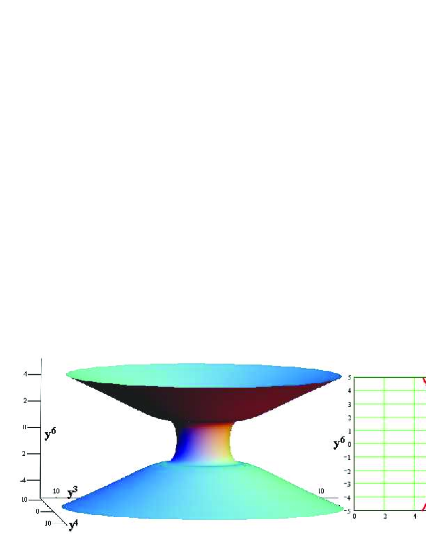
Figure 1: Manifold slices $y^{3}-y^{4}-y^{6}$, and $y^{1}-y^{6}$ at $t=\phi=\theta=0$. The manifold rotates in the $y^{1}-y^{2}$ plane.

The $y^{1}-y^{6}$ slice in this figure, appears as a line spinning in the $y^{1}-y^{2}$ plane at a rate of $\omega=\frac{c}{2k\,m}$. The tip of the curve corresponds to the event horizon, which is also at the waist of the $y^{3}-y^{4}-y^{6}$ slice. This tip is spinning at the speed of light. That is, the velocity vector becomes null at this point. The velocity of each point on the curve models the time dilation we see in a gravitational field, which the Minkowski space, $\mathbb{Y}$, takes care automatically.

The rotation of the manifold models acceleration. There are two components of this acceleration: an in-manifold component and an out-of-manifold component. The in-manifold component, which is in the $r$ direction, models the acceleration due to gravity.

Isochronal Embedding Methodology

Consider the line element for a static, spherically symmetric manifold:

$$ds^{2}=-c^{2}f^{2}\left(r\right)\,dt^{2}+g^{2}\left(r\right)\,dr^{2}+h^{2}\left(r\right)\,d\Theta^{2}$$ (4)

The first step is to define the isochronal, time-like function:

$$y^{0}=k_{1}\,c\,t,$$

where $k_{1}$ is a free parameter. We then remove that term from (4) leaving a Riemannian sub-metric, which we then embed.

We use an idea due to Kasner [4] as carried forward by Fronsdal [5] to create the function, $f$, while compensating for the term introduced by $y^{0}$:

$$y^{1} =2k_{2}\,m\,\sqrt{k_{1}^{2}-f^{2}}\,\cos\left(\frac{c\,t}{2k_{2}\,m}\right)$$ (5)

$$y^{2} =2k_{2}\,m\,\sqrt{k_{1}^{2}-f^{2}}\,\sin\left(\frac{c\,t}{2k_{2}\,m}\right)$$

The term, $m$, is included in the circular function arguments to balance units.

We ensure that $y^{1}$ and $y^{2}$ remain real by demanding $k_{1}^{2}\geq f^{2}$. The term, $k_{2}$, is a second free parameter.

The spherical term can be captured in the following three functions:

$$y^{3} =h\cos\left(\theta\right)\cos\left(\phi\right)$$ (6)

$$y^{4} =h\cos\left(\theta\right)\sin\left(\phi\right)$$

$$y^{5} =h\sin\left(\theta\right)$$

So far, we have a metric tensor that defines a line segment as:

$$ds^{2}=-c^{2}f^{2}\,dt^{2}+h^{2}\,d\Theta^{2}+\left[\left(h^{{}^{\prime}}\right)^{2}+\left(2k_{2}\,m\,\sqrt{k_{1}^{2}-f^{2}}^{{}^{\prime}}\right)^{2}\right]\,dr^{2}$$

Where the prime denotes differentiation with respect to $r$. We will use $y^{6}$ to correct the coefficient of $dr^{2}$:

$$y^{6}=\int\sqrt{g^{2}-\left(h^{{}^{\prime}}\right)^{2}-\left(2k_{2}\,m\,\sqrt{k_{1}^{2}-f^{2}}^{{}^{\prime}}\right)^{2}}\,dr$$ (7)

The requirement that each of these functions remain real, places constraints on the two free parameters, $k_{1}$ and $k_{2}$.

Note that the manifold is dynamic, even though the metric tensor is static. This is a general result: any isochronal manifold that admits a metric that has nonvanishing gravitational field must be dynamic. If it were not, there would be no acceleration due to gravity since the space-time we are embedding within is flat.

As demonstrated above, the Isochronal Embedding Method is applicable to metrics that can be placed in diagonal form with bounded, real functions, $f$, $g$ and $h$, and with $g^{2}-\left(h^{{}^{\prime}}\right)^{2}-\left(2k_{2}\,m\,\sqrt{k_{1}^{2}-f^{2}}^{{}^{\prime}}\right)^{2}$ everywhere non-negative for some fixed value of $k_{1}$ and $k_{2}$. While these constraints exclude a global embedding of the Schwarzschild metric, we can find a piece of a manifold that has the Schwarzschild metric (the piece outside the event horizon):

$$ds^{2} =-c^{2}\left(1-\frac{2m}{r}\right)\,dt^{2}+\frac{r}{r-2m}dr^{2}+r^{2}d\Theta^{2}$$ (8)

$$y^{0} =c\,t$$

$$y^{1} =2k\,m\,\sqrt{\frac{2m}{r}}\cos\left(\frac{c\,t}{2k\,m}\right)$$

$$y^{2} =2k\,m\,\sqrt{\frac{2m}{r}}\sin\left(\frac{c\,t}{2k\,m}\right)$$

$$y^{3} =r\cos\left(\phi\right)\cos\left(\theta\right)$$

$$y^{4} =r\sin\left(\phi\right)\cos\left(\theta\right)$$

$$y^{5} =r\sin\left(\theta\right)$$

$$y^{6} =\int\sqrt{\frac{r}{r-2m}-1-2k^{2}\frac{m^{3}}{r^{3}}}\,dr$$

We can see that the two manifolds, (3) and (8), are identical over their range of mutual validity – just use the transformation to isotropic coordinates[2]:

$$r=\left(1+\frac{m}{2R}\right)^{2}R$$

We can also see this qualitatively in Figure 2.

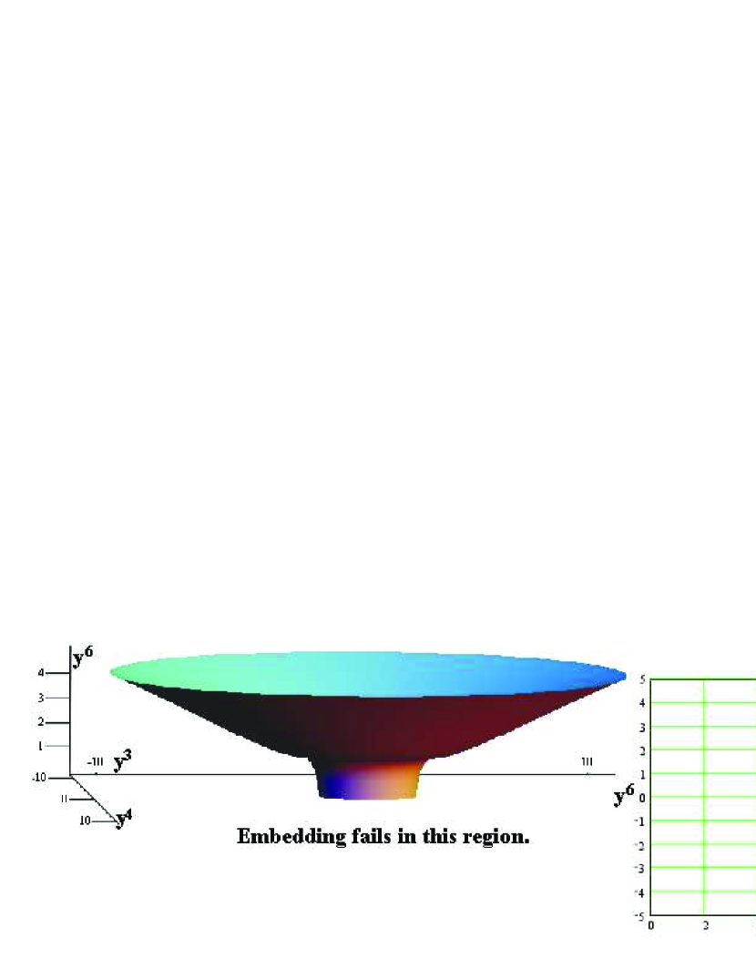
Figure 2: The manifold defined using the Schwarzschild metric (8) is identical to the one defined using (3) over the range of mutual validity. This embedding method fails at the event horizon because of the coordinate singularity in (8).

We can see clearly that embedding (8) fails at the event horizon, while embedding (3), does not. This offers a way to analytically continue a manifold in a natural way.

This example also shows that the manifold itself is coordinate-free. That is, the manifold image (as seen in Figures 1 and 2, in this case) is independent of the coordinate system used to express the metric (over the range of validity of the embedding).

Summary

We have demonstrated a method for decomposing certain semi-Riemannian metric tensors into a Riemannian tensor and an isochronal tensor. We have shown that we can embed the Riemannian portion in Euclidean space, $\mathbb{R}^{n}$, and then add a single time-like isochronal dimension to that space to create a $n+1$ Minkowski space. The resulting manifold, embedded in the Minkowski space, admits to the given metric tensor. The resulting manifold provides a particularly simple way to visualize the force and time dilation caused by gravity.

For this class of metric, the various embedding theorems that apply to Riemannian manifolds can be extended to apply to semi-Riemannian manifolds. And since there is considerable experience in the mathematical community with Riemannian manifolds, it is hoped that progress may be made applying other tools to metrics that admit to at least a local, isochronal embedding.

References

- [1] Dirac, P.A.M., General Theory of Relativity, (John Wiley & Sons, New York: 1975), p 11.
- [2] Stephani, H., General Relativity, An Introduction to the Theory of the Gravitational Field, (Cambridge University Press, New York: 1990), pp 113 - 114.
- [3] Dirac, P.A.M., op cit, pp 13, 14.
- [4] Kasner, Edward, Am. J. Math. No. 43, p 130 (1921)
- [5] Fronsdal, C., Phys Rev No. 116, p 778 (1959)