Quantum corrections to the Schwarzschild metric and reparametrization transformations

Abstract

Quantum corrections to the Schwarzschild metric generated by loop diagrams have been considered by Bjerrum-Bohr, Donoghue, and Holstein (BHD) [Phys. Rev. D68, 084005 (2003)], and Khriplovich and Kirilin (KK) [J. Exp. Theor. Phys. 98, 1063 (2004)]. Though the same field variables in a covariant gauge are used, the results obtained differ from one another. The reason is that the different sets of diagrams have been used. Here we will argue that the quantum corrections to metric must be independent of the choice of field variables, i. e. must be reparametrization invariant. Using simple reparametrization transformation, we will show that the contribution considered by BDH, is not invariant under it. Meanwhile the contribution of the complete set of the diagrams, considered by KK, satisfies the requirement of the invariance.

I General structure of reparametrization transformation

In the series of papers Weinberg Weinberg (1964a, b, 1965), Boulware and Deser Boulware and Deser (1975) have shown that the massless particles of helicity $\pm 2$ are described by the effective theory, satisfying the equivalence principle. Boulware and Deser have shown that the corresponding effective action coincides with the classical Einstein action 

$$\bar{S}_{g}=\int d^{4}x\left[-\sqrt{-\bar{g}}\,\bar{R}(\bar{g})\right].$$ (1)

In general case, it is necessary to supplement the lagrangian density with a number (may be infinite) of terms of higher orders in $\partial_{\alpha}\bar{g}_{\mu\nu}$. The natural property of any effective theory is the reparametrization invariance. It implies that a scattering amplitude on mass shell does not depend on the choice of field variables. In general relativity one of natural parametrizations of the gravitational field $h_{\alpha\beta}$ is the decomposition of the covariant metric tensor: $\bar{g}_{\mu\nu}=g_{\mu\nu}+f_{\mu\nu}(h)$, where $f$ is an arbitrary symmetric tensor function, the expansion of which begins with a linear in $h_{\alpha\beta}$ term. For example, to derive the counter lagrangian of the gravity, interacting with a massless scalar field, ’t Hooft and Veltman ’t Hooft and Veltman (1974) have used the trivial parametrization

$$\bar{g}_{\mu\nu}=g_{\mu\nu}+h_{\mu\nu},$$ (2)

where $g_{\mu\nu}$ is the background field, $h_{\mu\nu}$ is the operator field, characterizing quantum fluctuations. The action of scalar field in external gravitational field has the form

$$\bar{S}_{m}=\int d^{4}x\,\frac{\sqrt{-\bar{g}}}{2}\left(\bar{g}^{mn}\partial_{n}\bar{\phi}\,\partial_{m}\bar{\phi}-m^{2}\bar{\phi}^{2}\right).$$ (3)

Similarly to (2), we decompose the field $\bar{\phi}$

$$\bar{\phi}=\tilde{\phi}+\phi.$$ (4)

Supplementing the action (1) with a gauge fixing part

$$S_{f}=\int d^{4}x\,\frac{\sqrt{-g}}{2}\left(h_{\mu\mid\alpha}^{\alpha}{}-\frac{1}{2}h_{\mid\mu}\right)\left(h_{\mid\beta}^{\mu\beta}{}-\frac{1}{2}h^{\mid\mu}\right),$$ (5)

and a corresponding action of ghosts $\eta_{\mu}$, we find the expansion of the action up to second order in fluctuations:

$$\bar{S}_{g}+\bar{S}_{m}+S_{f}+S_{gh}(\eta)=\int d^{4}x\sqrt{-g}\left(\mathcal{L}+\underline{\mathcal{L}}+\underline{\underline{\mathcal{L}}}\right),$$ (6)

with

$$\mathcal{L} =-R+\frac{1}{2}\left(g^{\mu\nu}\partial_{\nu}\tilde{\phi}\,\partial_{\mu}\tilde{\phi}-m^{2}\tilde{\phi}^{2}\right),$$ (7)

$$\underline{\mathcal{L}} =\left(R_{\mu}^{\nu}-\frac{1}{2}\delta_{\mu}^{\nu}R-\frac{1}{2}T_{\mu}^{\nu}\right)h^{\mu}_{\nu}+\left(\tilde{\phi}_{\mid\lambda}^{\mid\lambda}+m^{2}\tilde{\phi}\right)\phi,$$ (8)

$$\underline{\underline{\mathcal{L}}} =-\frac{1}{4}\left(h_{\alpha\beta}P^{\alpha\beta}_{\gamma\delta}{}h^{\gamma\delta}{}_{\mid\lambda}^{\mid\lambda}+h_{\alpha\beta}X^{\alpha\beta}_{\gamma\delta}h^{\gamma\delta}\right),$$ (9)

$$+\frac{1}{4}h_{\alpha\beta}W^{\alpha\beta}_{\gamma\delta}h^{\gamma\delta}+\eta^{\dagger\,\mu}\left(\eta_{\mu}{}^{\mid\lambda}{}_{\mid\lambda}+R_{\mu}^{\lambda}\eta_{\lambda}\right),$$

$$+\phi\left(P^{\mu\nu}_{\gamma\delta}\partial_{\mu}\tilde{\phi}\,D_{\nu}+P^{\mu\nu}_{\gamma\delta}\tilde{\phi}_{\mid\mu\nu}-\frac{1}{2}\,g_{\gamma\delta}m^{2}\tilde{\phi}\right)h^{\gamma\delta}.$$

In expressions (7)-(9) indices are raised and lowered by means of the tensor $g_{\mu\nu}$, $R_{\mu\nu}$ and $R$ are the Ricci tensor and Riemann curvature of the background field, respectively. We introduce also the notation $h=h^{\lambda}_{\lambda}$. Indices following vertical lines denote covariant derivatives relative to the metric tensor $g_{\mu\nu}$. Matrices, appearing in the expressions (7)-(9), have the following form:

$$P_{\gamma\delta}^{\alpha\beta} =\delta_{(\gamma}^{\alpha}\delta_{\delta)}^{\beta}-\frac{1}{2}g^{\alpha\beta}g_{\gamma\delta}\,,$$ (10)

$$X^{\alpha\beta}_{\gamma\delta} =P^{\alpha\beta}_{\rho\sigma}\left[R_{(\gamma}{}^{\rho}{}_{\delta)}{}^{\sigma}+\delta^{\sigma}_{(\delta}\left(R^{\rho}_{\gamma)}-\frac{1}{2}\delta^{\rho}_{\gamma)}R\right)\right]$$

$$+(\alpha\beta\leftrightarrow\gamma\delta)\,,$$ (11)

$$W^{\alpha\beta}_{\gamma\delta} =T^{(\alpha}_{\sigma}\,P^{\sigma\beta)}_{\gamma\delta}+T_{(\gamma}^{\sigma}\,P_{\sigma\delta)}^{\alpha\beta}$$

$$+\frac{1}{2}P^{\alpha\beta}_{\gamma\delta}\left(m^{2}\tilde{\phi}^{2}-T\right).$$ (12)

In the expressions (10)-(12) indices with brackets are to be symmetrized. $T_{\mu\nu}$ is the stress tensor of the scalar field:

$$T_{\mu\nu}=\partial_{\mu}\tilde{\phi}\,\partial_{\nu}\tilde{\phi}-\,\frac{1}{2}\,g_{\mu\nu}\left(g^{\rho\sigma}\partial_{\rho}\tilde{\phi}\,\partial_{\sigma}\tilde{\phi}-m^{2}\tilde{\phi}^{2}\right).$$ (13)

The first variation of the action (8) eventually supply us with the equations of motion for the background fields:

$$R_{\mu\nu}-\frac{1}{2}\,g_{\mu\nu}R=\frac{1}{2}\,T_{\mu\nu}\,,$$ (14)

$$g^{\mu\nu}\tilde{\phi}_{\mid\mu\nu}+m^{2}\tilde{\phi}=0\,.$$ (15)

In LABEL:\cite[cite]{\@@bibref{Authors_Phrase1YearPhrase2}{missing}{\@@citephrase{(}}{\@@citephrase{)}}}Boulware1975 it has been shown that, at fixed gauge, the three graviton vertex is matched by the gravitational interaction with stress tensor of the classical free spin 2 field up to four parameters, corresponding to the reparametrization of the field $h_{\mu\nu}$ :

$$\bar{g}_{\mu\nu}=g_{\mu\nu}+h_{\mu\nu}+a_{1}\,h_{\mu\lambda}h^{\lambda}_{\nu}$$

$$+a_{2}\,h_{\mu\nu}h+a_{3}\,g_{\mu\nu}h^{\alpha}_{\beta}h_{\alpha}^{\beta}+a_{4}\,g_{\mu\nu}h^{2}.$$ (16)

Loop corrections to the scattering amplitude have been studied in Refs. Bjerrum-Bohr et al. (2003), Khriplovich and Kirilin (2004). Corrections concerned were proportional to $\ln|q^{2}|$, where $q^{2}$ is the transfer momentum squared. In particular, it was found that, after averaging over the fluctuations, corrections to the Schwarzschild metric appeared:

$$g_{\mu\nu}=g^{\mathrm{cl}}_{\mu\nu}+\underline{g}{}_{\mu\nu}\,,$$ (17)

where $g^{\mathrm{cl}}_{\mu\nu}$ is the classical Schwarzschild solution, $\underline{g}{}_{\mu\nu}$ is the quantum correction to it. Quite apparently, the leading corrections to metric must be independent of the way of parametrization of the field $h_{\mu\nu}$. Actually, being quadratic in fluctuations, additional terms in the parametrization (16) generate additional structures to $\underline{\underline{\mathcal{L}}}$ only due to replacement of the field $h_{\mu\nu}$ in the lagrangian density $\underline{\mathcal{L}}$, i. e., these structures vanish after taking into account the equations of motion (14). However, in perturbation theory it happens only if all diagrams have been taken into account. In LABEL:\cite[cite]{\@@bibref{Authors_Phrase1YearPhrase2}{missing}{\@@citephrase{(}}{\@@citephrase{)}}}Bjerrum-Bohr:2002ks only certain part of the diagrams have been considered, namely, the graviton propagator corrections and the corrections to one of the vertices (Fig. 1). As we will show, the contribution of these diagrams is not reparametrization invariant.

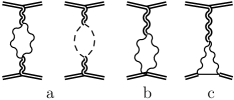
Figure 1: The diagrams taken into account in LABEL:\cite[cite]{\@@bibref{Authors_Phrase1YearPhrase2}{missing}{\@@citephrase{(}}{\@@citephrase{)}}}Bjerrum-Bohr:2002ks

II Example of reparametrization transformation

As an example, we parametrize the gravitational field in the following way

$$\bar{g}_{\mu\nu}=g_{\mu\nu}+h_{\mu\nu}-\frac{a}{4}\,h_{\mu\alpha}h^{\alpha}_{\nu}.$$ (18)

As stated above, the lagrangian quadratic in fluctuation changes due to the linear terms only. The reparametrization (18) is equivalent to the replacement of the matrices $X$ and $W$ in the lagrangian density (9) by the matrices $X+a\mathcal{X}$ and $W+a\mathcal{W}$, respectively, there

$$\mathcal{X}_{\gamma\delta}^{\alpha\beta} =\delta_{(\gamma}^{(\alpha}P^{\beta)}{}_{\delta),\kappa\lambda}R^{\kappa\lambda}\,,$$ (19)

$$\mathcal{W}_{\gamma\delta}^{\alpha\beta} =\frac{1}{2}\delta_{(\gamma}^{(\alpha}T_{\delta)}^{\beta)}\,.$$ (20)

Graviton propagator corrections are generated by the counter lagrangian of pure gravity. The counter lagrangian has been derived in LABEL:\cite[cite]{\@@bibref{Authors_Phrase1YearPhrase2}{missing}{\@@citephrase{(}}{\@@citephrase{)}}}Hooft1974, we aim here to find its transformation under the reparametrization transformation (18). Using the general formula for the counter lagrangian derived in LABEL:\cite[cite]{\@@bibref{Authors_Phrase1YearPhrase2}{missing}{\@@citephrase{(}}{\@@citephrase{)}}}Hooft1974, we find:

$$L_{count.}^{(a)} =\frac{\sqrt{-g}}{8\pi^{2}(d-4)}\frac{1}{4}\,Sp\left\{2a\left(X\mathcal{X}\right)\right.$$

$$\left.+\frac{a}{3}R\left(P\mathcal{X}\right)+a^{2}\left(P\mathcal{X}P\mathcal{X}\right)\right\}\,.$$ (21)

In the expression (21) the matrices $P,X$ and $\mathcal{X}$ should be read as $10\times 10$ matrices in relation to the number of the components of the symmetric tensor $h_{\mu\nu}$. Adding up the results of LABEL:\cite[cite]{\@@bibref{Authors_Phrase1YearPhrase2}{missing}{\@@citephrase{(}}{\@@citephrase{)}}}Hooft1974 and (21) yields the counter lagrangian for the case of pure gravity

$$L_{count.} =\frac{\sqrt{-g}}{8\pi^{2}(d-4)}\left[\left(\frac{7}{20}+\frac{a^{2}}{8}\right)R_{mn}R^{mn}\right.$$ (22)

$$\left.+\left(\frac{1}{120}+\frac{a}{8}\left(\frac{14}{3}+a\right)\right)R^{2}\right]\,.$$ (23)

This lagrangian gives the following corrections to the pure time component of the metric (diagram Fig. 1a):

$$\underline{g}{}^{\ref{f1}a}_{00}=-\left[\frac{43}{15}+a\left(\frac{14}{3}+2a\right)\right]\frac{G^{2}\hbar m}{\pi c^{5}r^{3}}\,.$$ (24)

Using the additional vertices (19), (20), it is easy to find the contributions of the diagrams depicted in Figs. 1b, c:

$$\underline{g}{}^{\ref{f1}b}_{00} =\left[\frac{26}{3}+a\left(\frac{37}{3}+2a\right)\right]\frac{G^{2}\hbar m}{\pi c^{5}r^{3}}\,,$$ (25)

$$\underline{g}{}^{\ref{f1}c}_{00} =-\left(\frac{5}{3}+5a\right)\frac{G^{2}\hbar m}{\pi c^{5}r^{3}}\,.$$ (26)

Summing up the results (24)-(26), we get the following contributions of the diagrams Fig. 1:

$$\underline{g}^{\ref{f1}a+\ref{f1}b+\ref{f1}c}_{00}=\left(\frac{62}{15}-\frac{2}{3}\,a\right)\frac{G^{2}\hbar m}{\pi c^{5}r^{3}}\,.$$ (27)

The a-independent part of Eq. (27) coincides with the result of LABEL:\cite[cite]{\@@bibref{Authors_Phrase1YearPhrase2}{missing}{\@@citephrase{(}}{\@@citephrase{)}}}Bjerrum-Bohr:2002ks. From Eq. (27) one can see that this contribution is not reparametrization invariant. Whereas the sum of the contributions of all the diagrams, listed in LABEL:\cite[cite]{\@@bibref{Authors_Phrase1YearPhrase2}{missing}{\@@citephrase{(}}{\@@citephrase{)}}}Khriplovich:2004cx, is reparametrization invariant for the obvious reason stated above

$$\underline{g}^{\mathrm{qu}}_{00}=\frac{107}{30}\frac{G^{2}\hbar m}{\pi c^{5}r^{3}}\,.$$ (28)

Parametrization dependence on the contribution of the diagrams Fig. 1 (i. e., diagrams containing a single graviton propagator attached to one of the particles) is the direct consequence of the fact that, in general relativity, separation of these diagrams from other loop ones is a matter of convention only, because they do not contain the pole in $q^{2}$ . Being unrelated to the renormalization of the amplitude with pole in $q^{2}$, these diagrams should be considered in line with other ones. As it has been shown, reparametrization transformations mix this diagrams with, for example, diagram proportional to $Sp\{PWPW\}$ (see Eqs. (10), (12)). Due to Eq. (14) there is no difference between the contribution of the diagrams Fig. 1 on mass shell and, for example, the diagram proportional to $Sp\{PWPW\}$.

III Aside on classical corrections

Figure 2: Tree diagrams

The correction (28) is the leading one in $l_{p}^{2}/r^{2}$, where $l_{p}$ is the Plank length. From the standpoint of leading corrections, the parametrizations (2), (18) are indeed indistinguishable, because, after averaging over the quantum fluctuation, the information about parametrization of these fluctuation is lost. Therein lies the main difference between the leading quantum corrections and nonleading classical corrections of the order $r^{2}_{g}/r^{2}$, there $r_{g}$ is the Schwarzschild radius. Let us consider this aspect in detail. The diagram depicted in Fig. 1c contributes to the classical correction to the Minkowski metric

$$\underline{\underline{g}}{}^{\mathrm{cl}}_{00}=(2+a)\,\frac{G^{2}m^{2}}{c^{4}r^{2}}\,.$$ (29)

However, this correction is actually induced by the tree diagram (Fig. 2a). The decomposition on the background field and its fluctuations (2) has no sense for such diagrams, because the integration momentum (flowing through the ”legs with crosses” in Fig. 2a) is of the order of $q$. It follows that the leading classical correction to the Minkowski metric

$$\underline{g}{}^{\mathrm{cl}}_{00}=-2\,\frac{Gm}{c^{2}r}$$ (30)

is of the same order as the field $h_{\mu\nu}$; consequently, it serves no purpose to distinguish them. Since the correction (29) is not the leading one, therefore it is possible to turn back to the initial variables (2) rather than (18), i. e.

$$\underline{\underline{g}}{}_{00}^{\mathrm{harm}}=\underline{\underline{g}}{}^{\mathrm{cl}}_{00}-\frac{a}{4}\left(\underline{g}{}^{\mathrm{cl}}_{00}\right)^{2}=\frac{2G^{2}m^{2}}{c^{4}r^{2}}\,,$$ (31)

where $\underline{\underline{g}}{}^{\mathrm{harm}}_{00}$ is the second order term in the expansion of the Schwarzschild metric in the harmonic coordinates.

It should be repeated once again that the quantum correction (28) is the leading one, therefore the trick (31) does not permit to turn back to the former variables, i. e, the correction must be invariant by itself. An important point is that $a$-dependent contributions to the potential vanish in the sum of the diagrams Fig. 2a and Fig. 2b only, i. e., even on the level of classical gravity one cannot introduce the physically meaningful ”one-particle-irreducible potential” (contrary to the section VIII of LABEL:\cite[cite]{\@@bibref{Authors_Phrase1YearPhrase2}{missing}{\@@citephrase{(}}{\@@citephrase{)}}}Bjerrum-Bohr:2002ks).